Gromov hyperbolicity and inner uniformity

Abstract.

In this paper, a characterization for inner uniformity of bounded domains in Euclidean $n$-space ${\mathbb{R}}^{n}$, $n\geq 2$, in terms of the Gromov hyperbolicity is established, as well as the quasisymmetry of the natural mappings between Gromov boundaries and inner metric boundaries of these domains. In particular, our results show that the answer to a related question, raised by Bonk, Heinonen and Koskela in 2001, is affirmative.

1. Introduction

The aim of this paper is to establish relationships between the following three properties: inner uniformity and Gromov hyperbolicity of Euclidean domains, and quasisymmetry of mappings related to such domains. These properties are very useful in the geometric function theory and geometric group theory, and they have been widely applied in the literature.

1.1. Gromov hyperbolicity

The Gromov hyperbolicity is a concept introduced by Gromov in the setting of geometric group theory in 1980s [35, 36]. Loosely speaking, this property means that a general metric space is “negatively curved”, in the sense of the coarse geometry. The concept generalizes a fundamental property of the hyperbolic metric, which has a constant negative Gaussian curvature. Unlike the Gaussian curvature, which is dependent on the two-dimensional surface theory, the concept of the Gromov hyperbolicity is applicable in a wide range of metric spaces. Because much of the classical geometric function theory can be built on the study of the geometry of the hyperbolic metric (see, e.g., [9]), it is hardly surprising that there are many connections to the generalizations of the other concepts originating from the classical function theory as well.

Indeed, since its introduction, the theory of the Gromov hyperbolicity has been found numerous applications, and it has been, for example, considered in the books [19, 21, 24, 28, 34, 66, 68]. Initially, the research was mainly focused on the hyperbolic group theory (see, e.g., [34]). Recently, researchers have shown an increasing interest in the study of the Gromov hyperbolicity from different points of view. For example, geometric characterizations of the Gromov hyperbolicity have been established in [4, 55]. Furthermore, the close connection between the Gromov hyperbolicity and quasiconformal deformations has been studied in [42]. The Gromov hyperbolicity of various metrics and surfaces has been investigated in [20, 39, 61, 65]. For other discussions in this line see, for example, [17, 18, 44, 76, 77].

1.2. Uniformity and inner uniformity

Uniform domains were independently introduced by John in [49] and by Martio and Sarvas in [60]. The importance of these domains in Euclidean spaces arises, for example, from their connections to various results in the theory of quasiconformal mappings [31, 71]. Motivated by these ideas, Bonk, Heinonen and Koskela introduced the concept of a uniform metric space in [14] and established a fundamental two-way correspondence between this class of spaces and proper, geodesic and Gromov hyperbolic spaces. Since its introduction, the concept of the uniformity has played a significant role in the study of geometric function theory in metric spaces, such as the properties of quasiconformal and quasimöbius mappings of metric spaces [22, 46, 78], the theory of Lipschitz and quasiconformal mappings of Carnot groups (including Heisenberg groups) [26, 29], boundary behavior and boundary extensions of Sobolev functions [1, 12, 30, 50], the Martin boundary in potential theory [2], the boundary Harnack principle for second order elliptic partial differential equations [53, 54], and even the Brownian motion in probability theory [5, 27].

Inner uniformity of a domain means that, for any two points in the domain, there exists a curve connecting these two points, which is neither “too long” (when compared with the inner distance of these two points) nor “too close” to the boundary of the domain with respect to its inner metric. It can be said that inner uniform domains are an intermediate class between uniform domains and John domains. Inner uniform domains were introduced in the plane by Balogh and Volberg in their study of the complex iteration of certain polynomials [7, 8], where they called these domains uniformly John domains. Inner uniform domains were also considered by Bonk, Heinonen and Koskela, who proved that every inner uniform domain in ${\mathbb{R}}^{n}$ is Gromov hyperbolic with respect to the quasihyperbolic metric [14, Theorem 1.11]. They also showed that a planar domain is Gromov hyperbolic with respect to the quasihyperbolic metric if and only if it is a conformal image of an inner uniform slit domain [14, Theorem 1.12]. For a comprehensive survey on inner uniformity and related concepts, see [74].

Recently, there has been substantial interest in study of inner uniformity. For example, invariance of inner uniformity under quasiconformal mappings in ${\mathbb{R}}^{n}$ has been investigated in [23]. A boundary Harnack principle in inner uniform domains has been established in [56, 57, 58]. Neumann and Dirichlet heat kernels on inner uniform domains have been considered in [37, 67].

1.3. Quasisymmetric mappings

Quasisymmetric mappings originate from the work of Beurling and Ahlfors [10], who defined them as the boundary values of quasiconformal self-mappings of the upper half-plane onto the real line. The general definition of quasisymmetry (see Definition 2.10 below) is due to Tukia and Väisälä, who introduced the general class of quasisymmetric mappings in [69]. Since its appearance, the concept has been studied by numerous authors. See, for example, [6, 48] for the properties of this class of mappings. Applications related to geometry and analysis in general metric spaces are discussed in [11, 52]. Relations of quasiconformality, quasisymmetry and the bi-Lipschitz property of mappings are investigated in [3, 40, 41, 45, 47, 70, 79].

In particular, Bonk and Merenkov employed quasisymmetric mappings in their investigation of the quasisymmetric rigidity, uniformization and the co-Hopfian property of Sierpiński carpets [13, 16, 63]. Furthermore, with the aid of this class of mappings, Bonk and Kleiner built the so-called Bonk-Kleiner program on quasisymmetric rigidity and uniformization of metric $2$-spheres with applications in geometric group theory and Gromov hyperbolic geometry [15]. See [64] for the recent developments in this line. In addition, this class of mappings has played a significant role, e.g., in study of complex analytic dynamics system [38, 62, 80] and Gromov hyperbolic spaces [25, 51, 59].

1.4. Gromov hyperbolicity and (inner) uniformity

The following result, concerning the relationship between Gromov hyperbolicity and uniformity, is due to Bonk, Heinonen and Koskela.

Theorem A. $($[14, Theorem 1.11]$)$ A bounded domain in ${\mathbb{R}}^{n}$ is uniform if and only if it is Gromov $\delta$-hyperbolic and its Euclidean boundary is naturally quasisymmetrically equivalent to the Gromov boundary.

See also [43, 75] for analogous results of Theorem in the settings of metric spaces and Banach spaces. Furthermore, in [14], Bonk, Heinonen and Koskela asked the question (see the second paragraph after [14, Theorem 1.11]):

Question 1.1.

Is there any result similar to Theorem for inner uniform domains?

The main purpose of this paper is to answer this question. We use two notions: Property and Property . Roughly speaking, Property stands for the combination of the Gromov hyperbolicity and the quasisymmetry of the correspondence between the Gromov boundary and the inner metric boundary of a domain in ${\mathbb{R}}^{n}$. Property is composed of the uniformity of the image space, the bi-Lipschitz property of the mapping with respect to the quasihyperbolic metric and the quasisymmetry of the corresponding boundary mapping (i.e., the restriction of the mapping on the boundary of the domain space). Precise definitions of these two properties and other related concepts will be given in Section 2. Our main result is the following:

Theorem 1.2.

Suppose $(G,|\cdot|)$ is a bounded domain in $\mathbb{R}^{n}$ and $\tau\in(0,\nu_{0}]$, where $|\cdot|$ denotes the Euclidean metric and $\nu_{0}$ is the constant of (3.2) below. Then, the following statements are equivalent.

1. $G$ is inner uniform;

2. The triple $[(G^{*},(k_{G})_{\tau}^{w_{0}}),(\overline{G_{\sigma}},\sigma);\varphi]$ has Property , where $w_{0}\in G$ satisfies (3.1) below;

3. The triple $[(\overline{G_{\sigma}},\sigma),(\overline{G_{(k_{G})_{\tau}}},(k_{G})_{\tau});f]$ has Property .

Remark 1.3.

The equivalence between (1) and (2) in Theorem 1.2 shows that the answer to Question 1.1 is affirmative.

1.5. Methodological novelty and significance

It can be said that this paper is built on the following fundamental ideas, all of which, to our belief, are new in this context:

1. In our view, the main obstacle to answering Question 1.1 is in showing the inner uniformity of the related domains directly from Property . The difficulty arises from the fact that, in Property , no conditions related to mappings in the interiors of the spaces are given, but the inner uniformity is a property that is defined in terms of the interior geometry of the domains. To overcome this difficulty, we introduce Property in Subsection 2.8.

   By comparing Property and Property , we see that in the latter the assumption of the Gromov hyperbolicity of the domain space in Property is replaced by the stronger one, i.e., uniformity of the image space. In addition, Property includes a condition that the mapping between the interiors of the spaces is bi-Lipschitz with respect to the quasihyperbolic metrics. In particular, Property guarantees that the image space is quasihyperbolically geodesic. These conditions are important in the proof of the inner uniformity of the related domains.

2. The proof of the implication from Property to Property (i.e., the implication from (2) to (3) in Theorem 1.2) is based on the construction of a homeomorphism which is quasihyperbolic (i.e., bi-Lipschitz with respect to quasihyperbolic metrics) on the interiors of the spaces and quasisymmetric on their boundaries. Note that it is usually very difficult to connect the boundary geometry of the domains to the interior one, and this is even harder when mainly quasihyperbolic metric, and related concepts, are used (instead of conformal modulus).

   In this paper, we construct such a homeomorphism by using the natural mappings in a new way (see the proof of Lemma 3.1 in Section 3). We reach this goal by three steps: Firstly, we construct a quasihyperbolic mapping in the interiors of the spaces, secondly, we construct a quasisymmetric mapping on their boundaries, and, thirdly, we prove that the mapping is a homeomorphism in the closures of the spaces.

3. A result in this paper, which we find somewhat surprising, is the inner uniformity of the preimage of a quasihyperbolic geodesic under the assumptions of Property . Four sections, Sections 4 $\sim$ 7, mainly deal with demonstrating this property. This guarantees the inner uniformity of the related domains, provided that the assumptions of Property are satisfied. In particular, this shows the implication from (3) to (1) in Theorem 1.2.

1.6. Organization of the paper

This paper is organized as follows. In Section 2, we introduce the necessary terminology, recall certain useful results, and show the equivalence of different definitions of rough starlikeness. In Section 3, the proofs of the implications (1) $\Longrightarrow$ (2) $\Longrightarrow$ (3) in Theorem 1.2 are presented (see Theorem 3.2 below). Furthermore, in the end of Section 3, certain frequently used constants are introduced. In Section 4, we show a series of lemmas which are used in the next three sections.

The discussions in Section 5 and Section 6 prepare for the proof of the main result, which will be given in Section 7. In Section 5, we check that the preimage of a quasihyperbolic geodesic satisfies the cigar condition with respect to diameter under the assumptions of Property (see Theorem 5.1), and, further, in Section 6, we show that Theorem 5.1 is also valid with respect to length (see Theorem 6.1 below).

In Section 7, the following assertion, which is based on Theorem 6.1, is established: If there is a homeomorphism $f:$ $(\overline{G_{\sigma}},\sigma)\to(\overline{Y_{d^{\prime}}},d^{\prime})$ such that the triple $[(\overline{G_{\sigma}},\sigma),(\overline{Y_{d^{\prime}}},d^{\prime});f]$ has Property , then $G$ is inner uniform (i.e., Theorem 7.1 below). Of particular note is that this assertion is independent of the dimension $n$ of the space. This means that the inner uniformity coefficient obtained in Theorem 7.1 depends only on the given data and is independent of the dimension $n$. As a direct consequence, we see that the implication (3) $\Longrightarrow$ (1) in Theorem 1.2 is true, and, hence, Theorem 1.2 follows.

2. Preliminaries

Let $(X,d)$ denote a metric space. A curve in $X$ is a continuous function $\gamma:\;I\to X$ from an interval $I\subset{\mathbb{R}}$ to $X$. If $\gamma$ is an embedding of $I$, it is also called an arc. We use $\gamma$ to denote both the function and its image set. The length $\ell_{d}(\gamma)$ of $\gamma$ with respect to the metric $d$ is defined in the usual way. The parameter interval $I$ is allowed to be closed, open or half-open. If $\ell_{d}(\gamma)<\infty$, then $\gamma$ is said to be rectifiable.

$(X,d)$ is called rectifiably connected if every pair of points in $X$ can be joined with a curve $\gamma$ in $X$ with $\ell_{d}(\gamma)<\infty$, and geodesic if every pair of points $x,$ $y$ in $X$ can be joined by a curve $\gamma$ with $\ell_{d}(\gamma)=d(x,y)$. For convenience, we always assume that $(X,d)$ and $(Y,d^{\prime})$ are locally compact, non-complete and rectifiably connected metric spaces.

2.1. Uniform spaces, inner uniform spaces and John spaces

Let $M\geq 1$ be a constant, and let $\gamma:$ $[0,1]\to X$ denote a curve with endpoints $x=\gamma(0)$ and $y=\gamma(1)$. Then, we say that $\gamma$ satisfies

1. $M$-cigar condition (with respect to $d$-length), if

   $$\min\{\ell_{d}(\gamma[x,z]),\ell_{d}(\gamma[z,y])\}\leq M\delta(d)_{X}(z)$$

   for any $z=\gamma(t)$, where $t\in[0,1]$ and $\gamma[x,z]$ denotes the part of $\gamma$ with endpoints $x$ and $z$;

2. $M$-turning condition (with respect to $d$-length) if $\ell_{d}(\gamma)\leq Md(x,y)$.

Here

$$\delta(d)_{X}(z)=d(z,\partial_{d}X)=\inf\{d(z,w):\;w\in\partial_{d}X\}$$

denotes the distance from $z$ to the metric boundary $\partial_{d}X$ of $X$ with respect to $d$, and $\partial_{d}X$ is the set

$$\partial_{d}X=\overline{X_{d}}-X,$$

where $\overline{X_{d}}$ stands for the metric completion. The assumptions guarantee that $\partial_{d}X$ is not empty. The definitions for cigar and turning conditions extend, in an obvious way, to the situations where the parameter interval is open or half open.

$(X,d)$ is called

1. $M$-John if any two points in $X$ can be joined by a curve in $X$ satisfying $M$-cigar condition;

2. $M$-uniform if any two points in $X$ can be joined by an $M$-uniform curve in $X$, where a curve is called $M$-uniform if it satisfies both $M$-cigar condition and $M$-turning condition.

The inner metric $\sigma(d)$ of $d$ is defined as follows: For any pair of points $x$ and $y$ in $X$,

$$\sigma(d)(x,y)=\inf\{\ell_{d}(\gamma)\},$$

where the infimum is taken over all rectifiable curves $\gamma$ in $X$ connecting $x$ and $y$. If $(X,\sigma(d))$ is $M$-uniform, then $(X,d)$ is called inner $M$-uniform. Similarly, we may define the concept of inner $M$-uniform curves.

Remark 2.1.

The following relations follow immediately from the definition: An $M$-uniform domain is inner $M$-uniform, and an inner $M$-uniform domain is $M$-John. Furthermore, $M$-John implies $M_{1}$-John when $M\leq M_{1}$. Similarly, (inner) $M$-uniformity of domains implies their (inner) $M_{1}$-uniformity for $M\leq M_{1}$.

Lemma 2.2.

For a domain $D$ in $X$, suppose $D$ is $M$-John with $M\geq 1$. Then, $D$ is bounded with respect to the metric $d$, if and only if it is bounded with respect to the inner metric $\sigma(d)$.

Proof. To prove this lemma, it suffices to show the necessity in the lemma since the sufficiency is obvious. For this, we let $x$, $y\in D$. Then, there is a curve $\gamma$ in $D$ connecting $x$ and $y$ such that for any $z\in\gamma$,

$$\min\{\ell_{d}(\gamma[x,z]),\ell_{d}(\gamma[z,y])\}\leq M\delta(d)_{D}(z).$$

Let $z_{0}\in\gamma$ bisect $\gamma$, i.e., $\ell_{d}(\gamma[x,z_{0}])=\ell_{d}(\gamma[y,z_{0}])$. Then, we see

$$\ell_{d}(\gamma)=2\ell_{d}(\gamma[x,z_{0}])\leq 2M\delta(d)_{D}(z_{0})\leq 2M{\operatorname{diam}}_{d}(D),$$

from which the necessity follows, where ${\operatorname{diam}}_{d}(D)$ denotes the diameter of $D$ with respect to $d$. ∎

We remark that the assumption that the domain $D$ is John of Lemma 2.2 is necessary, as illustrated by the following example:

Example 2.3.

Let $D\subset\mathbb{R}^{2}$ be the domain defined as follows:

1. $S=\{(x,y)\in\mathbb{R}^{2}:\;0<x<1,\;0<y<1\},$

2. $L_{n}=\{(x,y)\in\mathbb{R}^{2}:\;x=\frac{1}{2^{n}},\;0<y\leq\frac{2}{3}\}$, and

3. $K_{n}=\{(x,y)\in\mathbb{R}^{2}:\;x=\frac{1}{2^{n}}+\frac{1}{2^{n+2}},\;\frac{1}{3}\leq y<1\},$

where $n$ is a positive integer. Now, let

$$D=S-\bigcup_{n=1}^{\infty}(L_{n}\cup K_{n})$$

(see Figure 1). Then $D$ is bounded with respect to the Euclidean metric $|\cdot|$, but it is not bounded with respect to the inner metric $\sigma(|\cdot|)$.

Figure 1. The domain of Example 2.3.

2.2. Quasihyperbolic metrics

Gehring and Palka [33] introduced the quasihyperbolic metric of a domain in ${\mathbb{R}}^{n}$.

Definition 2.4.

The quasihyperbolic length of a rectifiable curve $\gamma$ in $(X,d)$ is the number:

$$\ell_{k(d)_{X}}(\gamma)=\int_{\gamma}\frac{|dz|}{\delta(d)_{X}(z)}.$$

For any $x$, $y$ in $X$, the quasihyperbolic distance $k(d)_{X}(x,y)$ between $x$ and $y$ is defined by

$$k(d)_{X}(x,y)=\inf\{\ell_{k(d)_{X}}(\gamma)\},$$

where the infimum is taken over all rectifiable curves $\gamma$ in $X$ with endpoints $x$ and $y$, and $|dz|$ denotes the length element with respect to the metric $d$. The resulting metric space $(X,k(d)_{X})$ is complete, proper and geodesic provided that the identity mapping ${\operatorname{id}}:$ $(X,d)\to(X,\sigma(d))$ is homeomorphic (cf. [14]).

For a rectifiable curve $\gamma$ in $X$ connecting $x$ and $y$, the following useful inequalities hold:

(2.1) $$\ell_{k(d)_{X}}(\gamma)\geq\log\Big{(}1+\frac{\ell_{d}(\gamma)}{\min\{\delta(d)_{X}(x),\delta(d)_{X}(y)\}}\Big{)},$$

and, thus,

(2.2) $$k(d)_{X}(x,y)\geq\log\Big{(}1+\frac{\sigma(d)(x,y)}{\min\{\delta(d)_{X}(x),\delta(d)_{X}(y)\}}\Big{)}\geq\Big{|}\log\frac{\delta(d)_{X}(x)}{\delta(d)_{X}(y)}\Big{|}.$$

Recall that a curve $\gamma$ connecting $x$ and $y$ is a quasihyperbolic geodesic if $\ell_{k(d)_{X}}(\gamma)=k(d)_{X}(x,y)$. Each subcurve of a quasihyperbolic geodesic is a quasihyperbolic geodesic. It is known that quasihyperbolic geodesics always exist in any domain in ${\mathbb{R}}^{n}$ (cf. [32, Lemma 1]). This is not true in arbitrary metric spaces (cf. [72, Example 2.9]).

For other basic properties of the quasihyperbolic metric, we refer to [32].

2.3. Quasigeodesics and quasigeodesic rays

We always assume that all curves and rays $\alpha$ in $(X,d)$ are rectifiable, i.e., $\ell_{d}(\alpha)<\infty$, where a ray in $X$ is a curve with one of its endpoints in $X$ and the other in $\partial_{d}X$.

For a given constant $\lambda\geq 1$, a curve or a ray $\gamma$ in $X$ is called $\lambda$-quasigeodesic if for any two points $u$ and $v$ in $\gamma$,

$$\ell_{k(d)_{X}}(\gamma[u,v])\leq\lambda k(d)_{X}(u,v).$$

Obviously, a $\lambda$-quasigeodesic (resp. a $\lambda$-quasigeodesic ray) is a quasihyperbolic geodesic (resp. a quasihyperbolically geodesic ray) if and only if $\lambda=1$.

In 1991, Väisälä established the following property concerning the existence of quasigeodesics in Banach spaces: Suppose that $D$ is a proper domain in a Banach space and $\lambda>1$ is a constant. Then, for any $x$ and $y$ in $D$, there is a $\lambda$-quasigeodesic in $D$ joining these two points ([73, Theorem 3.3]).

2.4. Conformal deformations, and Gromov hyperbolic domains and spaces

Let us recall the following conformal deformations which were introduced by Bonk, Heinonen and Koskela (cf. [14, Chapter $4$]). Fix a base point $p\in X$, and consider the family of conformal deformations of $X$ defined by the densities:

$$\rho(d)_{\varepsilon}(x)=e^{-\varepsilon d(x,p)}\;\;(\varepsilon>0).$$

For $u$, $v\in X$, let

$$(d)_{\varepsilon}(u,v)=\inf\int_{\gamma}\rho(d)_{\varepsilon}ds,$$

where the infimum is taken over all rectifiable curves $\gamma$ in $X$ connecting $u$ and $v$. Then, $(d)_{\varepsilon}$ are metrics on $X$. We denote the resulting metric spaces by $X_{\varepsilon}=(X,(d)_{\varepsilon})$.

Definition 2.5.

Suppose $\delta\geq 0$ is a constant. We say that

1. $(X,d)$ is Gromov $\delta$-hyperbolic if for all $x,$ $y,$ $z,$ $p\in X$,

   $$(x|y)_{p}\geq\min\{(x|z)_{p},(z|y)_{p}\}-\delta,$$

   where $(x|y)_{p}$ is the Gromov product defined by

   $$2(x|y)_{p}=d(x,p)+d(y,p)-d(x,y);$$

2. For a proper domain $D$ in $X$, $D$ is called Gromov $\delta$-hyperbolic if $(D,k(d)_{D})$ is Gromov $\delta$-hyperbolic.

Also, we say that a metric space is Gromov hyperbolic if it is Gromov $\delta$-hyperbolic for some $\delta\geq 0$. It is known that all (inner) uniform domains in ${\mathbb{R}}^{n}$ are Gromov $\delta$-hyperbolic with respect to the quasihyperbolic metric ([14, Theorem 1.11]).

We remark that the definition for the Gromov hyperbolicity in Definition 2.5(1) is equivalent to the one given below in geodesic metric spaces (cf. [25]).

Definition 2.6.

Let $(X,d)$ be geodesic and $\delta$ a nonnegative constant. Denote by $[x,y]$ any geodesic joining two points $x$ and $y$ in $X$. If all triples of geodesics $[x,y],$ $[y,z]$, $[z,x]$ in $X$ satisfy

$$d(w,[y,z]\cup[z,x])\leq\delta$$

for any $w\in[x,y]$, then $(X,d)$ is called Gromov $\delta$-hyperbolic. In other words, every geodesic triangle in $X$ is $\delta$-thin.

The following proposition says that the deformations $X_{\varepsilon}$ are uniform whenever $(X,d)$ is a proper, geodesic and Gromov hyperbolic space.

Theorem B. $($[14, Proposition $4.5$]$)$ There is a constant $\varepsilon_{0}=\varepsilon_{0}(\delta)>0$ such that for any $0<\varepsilon<\varepsilon_{0}$, the conformal deformation $X_{\varepsilon}$ of a proper, geodesic and Gromov $\delta$-hyperbolic space $(X,d)$ is a bounded $A(\delta)$-uniform space, where the notation $\varepsilon_{0}(\delta)$ means that the constant $\varepsilon_{0}$ depends only on $\delta$.

Definition 2.7.

Suppose $(X,d)$ is Gromov $\delta$-hyperbolic.

1. A sequence $\{x_{i}\}$ in $X$ is called a Gromov sequence if $(x_{i}|x_{j})_{p}\to\infty$ as $i,$ $j\to\infty;$

2. Two such sequences $\{x_{i}\}$ and $\{y_{j}\}$ are said to be equivalent if $(x_{i}|y_{i})_{p}\to\infty$ as $i\to\infty;$

3. The Gromov boundary $\partial^{*}X$ of $X$ is defined to be the set of all equivalent classes, and $X^{*}=X\cup\partial^{*}X$ is called the Gromov closure of $X$;

4. For $a\in X$ and $b\in\partial^{*}X$, the Gromov product $(a|b)_{p}$ of $a$ and $b$ is defined by

   $$(a|b)_{p}=\inf\big{\{}\liminf_{i\to\infty}(a|b_{i})_{p}:\;\{b_{i}\}\in b\big{\}};$$

5. For $a,$ $b\in\partial^{*}X$, the Gromov product $(a|b)_{p}$ of $a$ and $b$ is defined by

   $$(a|b)_{p}=\inf\big{\{}\liminf_{i\to\infty}(a_{i}|b_{i})_{p}:\;\{a_{i}\}\in a\;\;{\rm and}\;\;\{b_{i}\}\in b\big{\}}.$$

2.5. Visual metrics

Suppose $(X,d)$ is a Gromov $\delta$-hyperbolic space. For $p\in X$ and $\tau>0$, define

$$\rho_{p,\tau}(x,y)=e^{-\tau(x|y)_{p}}$$

for $x,$ $y\in X^{*}$ with convention $e^{-\infty}=0$. Then, it follows from [76, Proposition $5.16$] (see also [14, §3]) that there is a constant $\tau_{0}=\tau_{0}(\delta)>0$ such that for any $0<\tau<\tau_{0}$, one defines a function $(d)_{\tau}^{p}$ satisfying

$$(d)_{\tau}^{p}\leq\rho_{p,\tau}\leq 2(d)_{\tau}^{p},$$

where the function $(d)_{\tau}^{p}$ is a metametric on $X^{*}$, that is, it satisfies the axioms of a metric except that $(d)_{\tau}^{p}(x,x)$ may be positive. In fact, $(d)_{\tau}^{p}(x,y)=0$ if and only if $x=y\in\partial^{*}X$. Hence, $(d)_{\tau}^{p}$ defines a metric in $\partial^{*}X$, which is called the visual metric of $\partial^{*}X$.

The metametric $(d)_{\tau}^{p}$ defines a topology $\mathcal{T}^{*}$ in $X^{*}$. In this topology, the points of $X$ are isolated. For a sequence $\{x_{i}\}\in X$ and $a\in\partial^{*}X$, $(d)_{\tau}^{p}(a,x_{i})\to 0$ as $i\to\infty$ if and only if $\{x_{i}\}$ is a Gromov sequence and $\{x_{i}\}\in a$ (cf. [76, Lemma 5.3]).

2.6. Natural mappings

Let $(X,d)$ be a metric space and $D$ a proper domain in $X$.

Since the restriction $\mathcal{T}^{*}|_{D}$ is discrete, the identity mapping ${\operatorname{id}}:\;D\to D$ is continuous from the topology $\mathcal{T}^{*}$ to the metric topology of $D$. If it has a continuous extension

$$\varphi:\;\;(D^{*},(k(d)_{D})^{p}_{\tau})\to(\overline{D_{d}},d),$$

then we call $\varphi$ a natural mapping.

Suppose $E$ is a Banach space with metric $d$. The following two results, due to Väisälä, are useful:

Theorem C. $($[75, Lemma $2.22$]$)$ Suppose $D\subset E$ is a Gromov $\delta$-hyperbolic domain. Then, the natural mapping

$$\varphi:\;\;(D^{*},(k(d)_{D})^{p}_{\tau})\to(\overline{D_{d}},d)$$

exists if and only if every Gromov sequence $\overline{x}=\{x_{1},x_{2},\ldots\}$ in $(D,k(d)_{D})$ has a limit $\xi$ with respect to $d$. Moreover, for each $\eta\in\partial^{*}D$ and for any Gromov sequence $\overline{x}\in\eta$, $\overline{x}$ converges to $\xi\in\partial_{d}D$ in $(\overline{D_{d}},d)$ and $\xi=\varphi(\eta)$.

Theorem D. $($[75, Proposition $2.26$]$)$ Suppose $D\subset E$ is an $M$-uniform domain. Then, the natural mapping

$$\varphi:\;\;(D^{*},(k(d)_{D})^{p}_{\tau})\to(\overline{D_{d}},d)$$

exists and is bijective for any $\tau$ with $0<\tau\leq\min\{1,\tau_{0}\}$. Moreover, a sequence $\overline{x}=\{x_{1},x_{2},\ldots\}$ in $D$ converges to $\xi\in\partial_{d}D$ with respect to $d$ if and only if $\overline{x}$ is a Gromov sequence in $(D,k(d)_{D})$ and $\varphi(\eta)=\xi\in\partial_{d}D$, where $\eta\in\partial^{*}D$ with $\overline{x}\in\eta$.

2.7. Useful classes of mappings

Definition 2.8.

Let $f:$ $(X,d)\to(Y,d^{\prime})$ be a mapping (not necessarily continuous), and let $L\geq 1$ and $K\geq 0$ be constants. If $\sup_{w\in Y}\{d^{\prime}(w,f(X))\}<+\infty$ and for all $x,y\in X$,

$$L^{-1}d(x,y)-K\leq d^{\prime}(x^{\prime},y^{\prime})\leq Ld(x,y)+K,$$

then $f$ is called an $(L,K)$-roughly quasi-isometric mapping (cf. [17] or [43]), where $d^{\prime}(w,f(X))$ denotes the distance from the point $w$ to the image $f(X)$ of $X$ under $f$ with respect to $d^{\prime}$, and primes mean the images of points under $f$, for example, $x^{\prime}=f(x)$

An $(L,0)$-roughly quasi-isometric mapping is said to be$L$-quasi-isometric.

If we replace $(X,d)$ in Definition 2.8 by $(I,|\cdot|)$, where $I$ denotes an interval in ${\mathbb{R}}$, then $f$ is called an $(L,K)$-roughly quasi-isometric curve (cf. [76]).

Definition 2.9.

A homeomorphism $f:$ $(X,d)\to(Y,d^{\prime})$ is called $L$-quasihyperbolic, with $L\geq 1$, if

$$L^{-1}k(d)_{X}(x,y)\leq k(d^{\prime})_{Y}(x^{\prime},y^{\prime})\leq Lk(d)_{X}(x,y)$$

for all $x$, $y\in X$.

Obviously, a homeomorphism between two proper domains in metric spaces is $L$-quasihyperbolic if and only if it is $L$-quasi-isometric (or bi-Lipschitz) with respect to the corresponding quasihyperbolic metrics.

Definition 2.10.

Suppose $\eta$ is a homeomorphism from $[0,\infty)$ to $[0,\infty)$. A homeomorphism $f:$ $(X,d)\to(Y,d^{\prime})$ is said to be $\eta$-quasisymmetric if $d(a,x)\leq td(x,b)$ implies

$$d^{\prime}(a^{\prime},x^{\prime})\leq\eta(t)d^{\prime}(x^{\prime},b^{\prime})$$

for all $t\geq 0$ and for each triple $\{a,x,b\}$ in $X$.

If we assume that the inequality of Definition 2.10 holds for each triple $\{a,x,b\}$ in $X$, such that $x\in A$ or $\{a,b\}\subset A$, then $f$ is called $\eta$-quasisymmetric rel $A$.

The following two theorems due to Väisälä are used in Section 3:

Theorem E. $($[75, Theorem $2.39$]$)$ Suppose $D$ is a bounded $M$-uniform domain in a Banach space $E$ with a base point $p\in D$ such that

$$\delta(d)_{D}(x)\leq c\delta(d)_{D}(p)$$

for all $x\in D$, where $d$ denotes the metric in $E$. Then, the bijective natural mapping

$$\psi:\;\;(D^{*},(k(d)_{D})^{p}_{\mu})\to(\overline{D_{d}},d),$$

which exists by Theorem , is $\eta$-quasisymmetric rel $\partial^{*}D$ with respect to the metametric $(k(d)_{D})^{p}_{\mu}$ of $D^{*}$ and the metric $d$ of $\overline{D_{d}}$, where $0<\mu\leq\mu_{0},$ the function $\eta=\eta_{c,M,\mu}$ $($i.e., $\eta$ depends only on the given parameters $c,$ $M$ and $\mu)$, and $\mu_{0}=\mu_{0}(M)$.

A space is intrinsic if the distance between any two points in this space is always equal to the infimum of the lengths of all curves joining these two points. A mapping $f:$ $(X,d)\to(Y,d^{\prime})$ is weakly surjective if for any fixed $q\in Y$,

$$\limsup_{d^{\prime}(y,q)\to\infty}\frac{d^{\prime}(y,f(X))}{d^{\prime}(y,q)}<1.$$

Obviously, surjectivity implies weak surjectivity.

Theorem F. $($[76, Theorem $5.35$]$)$ Suppose that $(X,p)$ and $(Y,p^{\prime})$ are pointed intrinsic Gromov $\delta$-hyperbolic spaces and that $f:$ $X\to Y$ is a $(\lambda,\mu)$-roughly quasi-isometric mapping with $p^{\prime}=f(p)$. Then, $f$ has an extension

$$f^{*}:\;\;(X^{*},(d)^{p}_{\varepsilon})\to(Y^{*},(d^{\prime})^{p^{\prime}}_{\varepsilon}),$$

which is continuous, where $0<\varepsilon\leq\min\{1,\tau_{0}\}$, $d$ and $d^{\prime}$ denote the metrics in $X$ and $Y$, respectively. Moreover, if $f$ is weakly surjective, then the restriction

$$f^{*}|_{\partial^{*}X}:\;\;(\partial^{*}X,(d)^{p}_{\varepsilon})\to(\partial^{*}Y,(d^{\prime})^{p^{\prime}}_{\varepsilon})$$

is $\eta$-quasisymmetric with $\eta=\eta_{\delta,\lambda,\mu}$.

In the rest of this paper, $G$ is always a proper subdomain of ${\mathbb{R}}^{n}$. Since $k(\sigma(d))_{G}=k(d)_{G}$ when $d=|\cdot|$, the Euclidean metric, if there is no danger of confusion, we simply use $k_{G}$ to denote both of them. In addition, we use the notations $\sigma$ and $\partial G$ instead of $\sigma(|\cdot|)$ and $\partial_{|\cdot|}G$, respectively.

2.8. Property A and Property B

Now, we are ready to give the precise definitions of Property and Property .

Property A. We say that the triple $[(G^{*},(k_{G})_{\tau}^{w}),(\overline{G_{\sigma}},\sigma);\varphi]$ has Property if the following statements hold:

1. $(G,k_{G})$ is Gromov $\delta$-hyperbolic, and

2. there are a point $w\in G$ and a bijective natural mapping

   $$\varphi:\;(G^{*},(k_{G})_{\tau}^{w})\to(\overline{G_{\sigma}},\sigma)$$

   such that the restriction $\varphi|_{\partial_{\sigma}G}:$ $(\partial^{*}G,(k_{G})_{\tau}^{w})\to(\partial_{\sigma}G,\sigma)$ is $\eta$-quasisymmetric, where $\tau\in(0,\nu_{0})$ (see Section 3 for the definition of $\nu_{0}$).

Property B. We say that the triple $[(\overline{G_{\sigma}},\sigma),(\overline{Y_{d^{\prime}}},d^{\prime});f]$ has Property if there are a constant $M\geq 1$ and a homeomorphism $f:$ $(\overline{G_{\sigma}},\sigma)\to(\overline{Y_{d^{\prime}}},d^{\prime})$ such that the following statements hold:

1. $(\overline{Y_{d^{\prime}}},d^{\prime})$ is a metric space and $(Y,d^{\prime})$ is $M$-uniform;

2. the restriction $f|_{G}:$ $(G,\sigma)\to(Y,d^{\prime})$ is $M$-quasihyperbolic, and

3. the restriction $f|_{\partial_{\sigma}{G}}:$ $(\partial_{\sigma}{G},\sigma)\to(\partial_{d^{\prime}}{Y},d^{\prime})$ is $\eta$-quasisymmetric.

2.9. Rough starlikeness

Let $(X,d)$ be an intrinsic Gromov $\delta$-hyperbolic space, and let $\mu$ and $h$ be nonnegative constants. A $(\mu,h)$-road $\overline{\alpha}$ in $X$ is a sequence of arcs $\alpha_{i}$ with endpoints $y_{i}$ and $u_{i}$ along the direction from $y_{i}$ to $u_{i}$ satisfying the following:

1. Each $\alpha_{i}$ is $h$-short;

2. The sequence of lengths $\ell_{d}(\alpha_{i})$ is increasing and tending to $\infty$;

3. For $i\leq j$, the length mapping $g_{ij}:\alpha_{i}\to\alpha_{j}$ with $g_{ij}(y_{i})=y_{j}$ satisfies $d(g_{ij}(x),x)\leq\mu$ for all $x\in\alpha_{i}$.

Here for $x$ and $y\in X$ and $h\geq 0$, a curve $\gamma$ in $X$ connecting $x$ and $y$ is called $h$-short if

$$\ell_{d}(\gamma)\leq d(x,y)+h.$$

By [76, Lemma 6.3], we see that for a $(\mu,h)$-road $\overline{\alpha}$ which consists of the arcs $\alpha_{i}$ connecting $y_{i}$ and $u_{i}$ along the direction from $y_{i}$ to $u_{i}$, the corresponding sequence $\{u_{i}\}$ is Gromov and defines a point $b$ in $\partial^{*}X$. If, further, for each $i$, $y_{i}=y$, then we say that $\overline{\alpha}$ is a road connecting $y$ and $b$.

Definition 2.11.

Let $(X,d)$ be a Gromov $\delta$-hyperbolic space, and let $K$, $\mu$ and $h$ be nonnegative constants. We say that $X$ is

1. $(K,\mu,h)$-roughly starlike with respect to a base point $w\in X$ if for any $x\in X$, there is a $(\mu,h)$-road $\overline{\alpha}$ connecting $w$ and $b\in\partial^{*}X$ such that $d(x,\overline{\alpha})\leq K$;

2. $(K,\mu)$-roughly starlike with respect to a base point $w\in X$ if it is $(K,\mu,h)$-roughly starlike with respect to $w$ for all $h>0$.

Definition 2.12.

A proper, geodesic and Gromov $\delta$-hyperbolic space $(X,d)$ is said to be $K$-roughly starlike $(K\geq 0)$ with respect to a base point $w\in X$ if for each point $x\in X$, there exists a geodesic ray $\beta$ starting from $w$ such that $d(x,\beta)\leq K$.

In the following, we shall prove that the above definitions for rough starlikeness are equivalent in proper, geodesic and Gromov hyperbolic spaces. First, let us recall a result due to Väisälä.

Theorem G. $($[76, Theorem $6.32$]$)$ Suppose that $(X,d)$ is an intrinsic Gromov $\delta$-hyperbolic space. Let $\varphi:[0,\infty)\to X$ be a $(\lambda,\mu)$-roughly quasi-isometric curve, and let $\overline{\alpha}$ be a $(\mu,h)$-road connecting $\varphi(0)$ and $\varphi(\infty)$. Then,

$$d_{H}(|\overline{\alpha}|,{\rm Im}\;\varphi)\leq M,$$

where $d_{H}$ stands for the Hausdorff distance, $``{\rm Im}"$ means the image set and $M=M(\delta,\lambda,\mu,h)$.

If a condition $\varpi$ with data $\chi$ implies a condition $\varpi^{\prime}$ with data $\chi^{\prime}$ so that $\chi^{\prime}$ depends only on $\chi$ and other given quantities, then we say that $\varpi$ implies $\varpi^{\prime}$ quantitatively. If also $\varpi^{\prime}$ implies $\varpi$ quantitatively, then we say that $\varpi$ and $\varpi^{\prime}$ are quantitatively equivalent. Different instances of $\varpi$ and $\varpi^{\prime}$ need not have the same value.

Lemma 2.13.

Suppose $(X,d)$ is a proper, geodesic and Gromov $\delta$-hyperbolic space. Then, the following are quantitatively equivalent:

1. $X$ is $(K_{1},\mu_{1},h_{1})$-roughly starlike;

2. $X$ is $(K_{2},\mu_{2})$-roughly starlike;

3. $X$ is $K_{3}$-roughly starlike.

Proof. Since [76, Lemma $6.34(1)$] implies that the conditions (1) and (2) in the lemma are quantitatively equivalent, and since the implication from (3) to (1) is obvious, we see that we only need to show the implication from (1) to (3). To this end, we let $w\in X$. Then, the assumption guarantees that there is a $(\mu_{1},h_{1})$-road $\overline{\alpha}$ connecting $w$ and $b\in\partial^{*}X$ with $d(w,\overline{\alpha})\leq K_{1}$. Furthermore, it follows from Hopf-Rinow Theorem that there is a geodesic ray $\beta$ connecting $w$ and $b$ (cf. [21, Lemma 3.1 in Part III-H]). Thus, by Theorem , we observe that there is a constant $M=M(\delta,\mu_{1},h_{1})$ such that $d_{H}(|\overline{\alpha}|,\beta)\leq M$, which leads to $d(w,\beta)\leq M+K_{1}$. Now, the lemma follows by letting $K_{3}=M+K_{1}$. ∎

Recall the following results, which are useful in Section 3.

Theorem H. $($[75, Theorem 3.22]$)$ Every Gromov $\delta$-hyperbolic domain in Banach spaces is $(K,\mu)$-roughly starlike with respect to each point in this domain, where $K=K(\delta)$ and $\mu=4\delta+1$.

Theorem I. $($[14, Proposition $4.37$]$)$ If $(G,d)$ is a $K$-roughly starlike, proper, geodesic and Gromov $\delta$-hyperbolic space, then for any $0<\varepsilon\leq\varepsilon_{0}$, the identity mapping from $(G,d)$ to $(G,k((d)_{\varepsilon})_{G})$ is homeomorphic and $L_{0}$-quasi-isometric, where $L_{0}=L_{0}(K,\delta,\varepsilon)$.

Theorem J. $($[14, Theorem $3.6$]$)$ If $(G,d)$ is a uniform space, then $(G,k(d)_{G})$ is a proper, geodesic and Gromov $\delta$-hyperbolic space. Moreover, if $G$ is bounded, then $(G,k(d)_{G})$ is roughly starlike and the quasisymmetric gauge determined by $d$ on $\partial_{d}G$ is naturally equivalent to the canonical gauge on the Gromov boundary $\partial^{*}G$.

Note that the canonical gauge in Theorem consists of visual metrics on $\partial^{*}G$. See [14] for the details.

We also make the following notational convention: The metric $d$ will be dropped from all related notations. For example, we write $k(d)_{X}=k_{X}$, $\ell_{d}=\ell$, $\delta(d)_{X}=\delta_{X}$, and so on.

3. Implications (1) $\Longrightarrow$ (2) $\Longrightarrow$ (3) in Theorem 1.2

The purpose of this section is twofold. We first prove the implications (1) $\Longrightarrow$ (2) $\Longrightarrow$ (3) in Theorem 1.2. Furthermore, we define certain constants which will be frequently used in this paper.

3.1. Proofs of the implications (1) $\Longrightarrow$ (2) and (2) $\Longrightarrow$ (3)

We assume that $(G,|\cdot|)$ is bounded. Let $w_{0}\in G$ be such that

(3.1) $$\delta(\sigma)_{G}(w_{0})=\sigma(w_{0},\partial_{\sigma}G)=\max\{\delta(\sigma)_{G}(x):\;x\in G\},$$

and let

(3.2) $$\nu_{0}=\min\{1,\varepsilon_{0},\;\tau_{0},\;\mu_{0}\},$$

where $\varepsilon_{0}$ (resp. $\tau_{0}$, $\mu_{0}$) is defined by Theorem (resp. Subsection 2.5, Theorem ).

Note that in Lemma 3.1 and its proof below, unless stated otherwise, we use the symbol $\eta$ (resp. the symbols $\delta$ and $K$) to denote the coefficient function of quasisymmetry (resp. the coefficients of Gromov hyperbolicity and starlikeness). We also use $M$ to denote the coefficient of uniformity or quasi-isometry or quasihyperbolicity. Particular instances of these functions and constants need not be the same, as these functions and constants depend on given assumptions and data.

Lemma 3.1.

Suppose the triple $[(G^{*},(k_{G})_{\tau}^{w_{0}}),(\overline{G_{\sigma}},\sigma);\varphi]$ has Property , where $\tau\in(0,\nu_{0})$. Then, the triple $[(\overline{G_{\sigma}},\sigma)\to\big{(}\overline{G_{(k_{G})_{\tau}}},(k_{G})_{\tau}\big{)};f]$ has Property , i.e., there exist a constant $M\geq 1$ and a homeomorphism $f:$ $(\overline{G_{\sigma}},\sigma)\to\big{(}\overline{G_{(k_{G})_{\tau}}},(k_{G})_{\tau}\big{)}$ such that the following statements hold:

1. $(G,(k_{G})_{\tau})$ is an $M$-uniform space;

2. the restriction $f|_{G}={\operatorname{id}}:$ $(G,\sigma)\to(G,(k_{G})_{\tau})$ is $M$-quasihyperbolic, and

3. the restriction $f|_{\partial_{\sigma}G}:$ $(\partial_{\sigma}G,\sigma)\to(\partial_{(k_{G})_{\tau}}G,(k_{G})_{\tau})$ is $\eta$-quasisymmetric.

Proof. Before the construction of the required homeomorphism, we need some preparation. We start with the claim:

Claim 3.1.

The metric space $(G,k_{G})$ is $K$-roughly starlike, complete, proper, geodesic and Gromov $\delta$-hyperbolic.

Obviously, the identity mapping $(G,|\cdot|)\to(G,\sigma)$ is a local isometric homeomorphism. We see from [14, Proposition 2.8] that $(G,k_{G})$ is complete, proper, geodesic and Gromov $\delta$-hyperbolic. Since the rough starlikeness of $(G,k_{G})$ follows from Lemma 2.13 and Theorem , the claim is proved.

It follows from Claim 3.1 and Theorem that

Claim 3.2.

The metric space $(G,(k_{G})_{\tau})$ is bounded and $M$-uniform.

Then, Claim 3.2 and Theorem guarantee the following:

Claim 3.3.

The metric space $\big{(}G,k\big{(}(k_{G})_{\tau}\big{)}_{G}\big{)}$ is $K$-roughly starlike, proper, geodesic and Gromov $\delta$-hyperbolic.

Now, we are ready to start the construction of the required homeomorphism. First, it follows from Claim 3.1 and Theorem that

$${\operatorname{id}}_{1}:\;(G,k_{G})\to\big{(}G,k\big{(}(k_{G})_{\tau}\big{)}_{G}\big{)}$$

is homeomorphic and $M$-quasi-isometric. Hence, by Theorem , Claim 3.1 and Claim 3.3, we see that there exists a bijective natural mapping

$${\operatorname{id}}_{1}^{*}:\;(G^{*},(k_{G})_{\tau}^{w_{0}})\to\Big{(}G^{*},\Big{(}k\big{(}(k_{G})_{\tau}\big{)}_{G}\Big{)}_{\tau}^{w_{0}}\Big{)}$$

such that the restriction

$${\operatorname{id}}_{1}^{*}|_{\partial^{*}G}:\;(\partial^{*}G,(k_{G})_{\tau}^{w_{0}})\to\Big{(}\partial^{*}G,\Big{(}k\big{(}(k_{G})_{\tau}\big{)}_{G}\Big{)}_{\tau}^{w_{0}}\Big{)}$$

is $\eta$-quasisymmetric.

Moreover, it follows from Claim 3.2 and Theorem that there is a bijective natural mapping

(3.3) $$\psi:\;\Big{(}G^{*},\Big{(}k\big{(}(k_{G})_{\tau}\big{)}_{G}\Big{)}_{\tau}^{w_{0}}\Big{)}\to\big{(}\overline{G_{(k_{G})_{\tau}}},(k_{G})_{\tau}\big{)}.$$

In order to exploit Theorem , we note the following relationship between the distance from $w_{0}$ to $\partial_{(k_{G})_{\tau}}G$ and the diameter of $G$ with respect to $(k_{G})_{\tau}$:

$$\delta((k_{G})_{\tau})_{G}(w_{0}) \geq \frac{1}{\tau e}\rho(k_{G})_{\tau}(w_{0})$$

$$\geq \frac{1}{2e}{\operatorname{diam}}_{(k_{G})_{\tau}}(G),$$

where the first inequality follows from [14, $(4.6)$], and the second one from the inequality next to [14, $(4.3)$]. Hence, for all $x\in G$,

$$\delta((k_{G})_{\tau})_{G}(x)\leq 2e\,\delta((k_{G})_{\tau})_{G}(w_{0}).$$

Thus, we see from Theorem that the restriction

$$\psi|_{\partial^{*}G}:\;\Big{(}\partial^{*}G,\Big{(}k\big{(}(k_{G})_{\tau}\big{)}_{G}\Big{)}_{\tau}^{w_{0}}\Big{)}\to(\partial_{(k_{G})_{\tau}}G,(k_{G})_{\tau})$$

is $\eta$-quasisymmetric.

Let

$$f_{1}=\psi\circ{\operatorname{id}}_{1}^{*}\circ\varphi^{-1}|_{\partial_{\sigma}G}:\;(\partial_{\sigma}G,\sigma)\to(\partial_{(k_{G})_{\tau}}G,(k_{G})_{\tau}).$$

Since a composition of $\eta$-quasisymmetric mappings is still $\eta$-quasisymmetric, $f_{1}$ is $\eta$-quasisymmetric. Furthermore, let ${\operatorname{id}}_{2}:$ $(G,\sigma)\to(G,k_{G})$ and ${\operatorname{id}}_{3}:$ $(G,(k_{G})_{\tau})\to(G,k((k_{G})_{\tau})_{G})$ be two identity mappings. Then, it follows from [14, Proposition 2.8] and the uniformity of $(G,(k_{G})_{\tau})$ in Claim 3.2 that both ${\operatorname{id}}_{2}$ and ${\operatorname{id}}_{3}$ are homeomorphic. Let

$$f_{2}={\operatorname{id}}_{3}^{-1}\circ{\operatorname{id}}_{1}\circ{\operatorname{id}}_{2}:\;(G,\sigma)\to(G,(k_{G})_{\tau}).$$

Then, this identity mapping is again homeomorphic. Furthermore, we see that $f_{2}$ is $M$-quasihyperbolic, since ${\operatorname{id}}_{1}$ is $M$-quasi-isometric. Let

$$f:\;(\overline{G_{\sigma}},\sigma)\to\big{(}\overline{G_{(k_{G})_{\tau}}},(k_{G})_{\tau}\big{)}$$

be defined as follows:

$$f|_{G}=f_{2}\;\;\mbox{and}\;\;f|_{\partial_{\sigma}G}=f_{1}.$$

It remains to prove that the mapping $f$ is homeomorphic. Because $f$ is bijective, it is sufficient to verify the continuity of $f$ and $f^{-1}$. First, we prove the claim:

Claim 3.4.

Suppose $\overline{x}=\{x_{n}\}\subset G$, $\eta\in\partial^{*}G$ and $\xi\in\partial_{\sigma}G$ with $\varphi(\eta)=\xi$, where $\varphi$ is from the assumption in the lemma. Then, $\sigma(x_{n},\xi)\to 0$ as $n\to\infty$, if and only if $\overline{x}$ is a Gromov sequence in $(G,k_{G})$ and $\overline{x}\in\eta$.

The sufficiency in the claim follows from the assumption of the lemma and Theorem . It remains to check the necessity part of the claim.

Assume that $\sigma(x_{n},\xi)\to 0$ as $n\to\infty$. We assert that $\overline{x}$ is a Gromov sequence in $(G,k_{G})$. To prove this assertion, let $\alpha_{n,m}$ be a quasihyperbolic geodesic in $G$ connecting $x_{n}$ and $x_{m}$. Then, it follows from the assumption of the lemma and the Gehring-Hayman condition (cf. [55, Theorem 1.1]) that there exists a constant $C>0$ such that for any natural integers $n$ and $m$,

$$\ell(\alpha_{n,m})\leq C\sigma(x_{n},x_{m}).$$

Moreover, by Claim 3.1 and [14, $(3.2)$], we see that there is a point $z_{n,m}\in\alpha_{n,m}$ such that

$$(x_{n}|x_{m})_{w_{0}}\geq k_{G}(z_{n,m},w_{0})-8\delta\geq\Big{|}\log\frac{\delta(\sigma)_{G}(w_{0})}{\delta(\sigma)_{G}(z_{n,m})}\Big{|}-8\delta.$$

Since

$$\delta(\sigma)_{G}(z_{n,m})\leq\sigma(z_{n,m},\xi)\leq\ell(\alpha_{n,m})+\sigma(x_{n},\xi)\leq C\sigma(x_{n},x_{m})+\sigma(x_{n},\xi)\to 0,$$

as $n,m\to\infty$, we obtain

$$(x_{n}|x_{m})_{w_{0}}\to\infty,$$

and, hence, the assertion is true. It follows that there is a $\zeta\in\partial^{*}G$ such that $\overline{x}\in\zeta$. Since $\varphi$ is bijective, we see from Theorem that $\zeta=\eta$, which gives the sufficiency part of the claim.

Now, we are ready to prove the lemma. Let $\xi\in\partial_{\sigma}G$ and $\overline{x}=\{x_{n}\}\subset G$. By Claim 3.4, we know that $\sigma(x_{n},\xi)\to 0$ as $n\to\infty$, if and only if $\overline{x}$ is a Gromov sequence in $(G,k_{G})$ and $\overline{x}\in\eta_{1}$, where $\eta_{1}=\varphi^{-1}(\xi)$. Moreover, by Claim 3.1 and Claim 3.3 along with the fact that ${\operatorname{id}}_{1}$ is homeomorphic and $M$-quasi-isometric, we see from [17, Proposition $6.3$] that $\overline{x}$ is a Gromov sequence in $(G,k_{G})$ and $\overline{x}\in\eta_{1}$, if and only if $\overline{x}$ is a Gromov sequence in $(G,k((k_{G})_{\tau})_{G})$ and $\overline{x}\in\eta_{2}$, where $\eta_{2}={\operatorname{id}}_{1}^{*}(\eta_{1})$.

Furthermore, it follows from Claim 3.2 and Theorem that $\overline{x}$ is a Gromov sequence in $(G,k((k_{G})_{\tau})_{G})$ and $\overline{x}\in\eta_{2}$, if and only if $(k_{G})_{\tau}(x_{n},\xi_{1})\to 0$, where $\xi_{1}=\psi(\eta_{2})$ and $\psi$ is from (3.3). Since $\xi_{1}=f(\xi)$, we see that both $f$ and $f^{-1}$ are continuous. Hence, the proof of the lemma is complete. ∎

Since the inverse of an $\eta$-quasisymmetric mapping is still $\eta$-quasisymmetric, we see that the following result follows immediately from (3.1), Lemma 2.2 and Lemma 3.1, Theorem and Theorem .

Theorem 3.2.

The implications (1) $\Longrightarrow$ (2) $\Longrightarrow$ (3) in Theorem 1.2 hold.

3.2. Frequently used constants

The constants given below will be frequently used in this paper.

$$A_{0}=\max\{e^{B_{0}^{2}M_{0}},(M_{1}\eta(B_{0}^{2}))^{M_{0}}\},\;\;B_{0}=20M_{0}^{2},\;\;M_{0}=\max\{e^{C_{1}M_{1}},\eta(C_{1}M_{1}^{2})\},$$

$$M_{1}=\max\Big{\{}\eta(M_{2}^{5}),e^{MM_{2}^{5}},\big{(}\eta^{-1}(M_{2}^{-1})\big{)}^{-1}M_{2}\Big{\}}$$

and

$$M_{2}=10C_{1}^{4}\eta(C_{1})\max\Big{\{}1,\big{(}\eta^{-1}(\frac{1}{5}C^{-3})\big{)}^{-1}\Big{\}},$$

where $\eta:$ $[0,\infty)\to[0,\infty)$ is a homeomorphism with $\eta(1)\geq 1$, $C_{1}=e^{4(CM)^{2}}$, $C$ denotes the uniformity coefficient of curves, $M$ stands for the uniformity coefficients of spaces and also for the quasi-isometry coefficients or quasihyperbolicity coefficients of mappings with $37\leq M+1\leq C$ (see Remark 4.4 for the definition of the constant $C$).

4. Auxiliary lemmas

The purpose of this section is to establish a series of lemmas which will be used later. We call $(X,d)$ strongly weakly geodesic if for any $x\in X$, the metric ball $\mathbb{B}(x,\delta_{X}(x))$ is geodesic. Obviously, $(G,|\cdot|)$ and $(G,\sigma)$ are strongly weakly geodesic.

Lemma 4.1.

Suppose $(X,d)$ is strongly weakly geodesic. For $x_{1}$ and $x_{2}$ in $X$, if $d(x_{1},x_{2})\leq a^{-1}\delta_{X}(x_{1})$ with $a>1$, then

$$k_{X}(x_{1},x_{2})\leq\frac{ad(x_{1},x_{2})}{(a-1)\delta_{X}(x_{1})}\leq(a-1)^{-1}.$$

Proof. Let $\alpha$ be a geodesic in $X$ connecting $x_{1}$ and $x_{2}$. Since for any $x\in\alpha$,

$$\delta_{X}(x)\geq\delta_{X}(x_{1})-d(x_{1},x_{2})>(a-1)a^{-1}\delta_{X}(x_{1}),$$

we have

$$k_{X}(x_{1},x_{2})\leq\int_{\alpha}\frac{|dx|}{\delta_{X}(x)}\leq\frac{ad(x_{1},x_{2})}{(a-1)\delta_{X}(x_{1})}\leq(a-1)^{-1},$$

as required. ∎

Lemma 4.2.

Suppose $x_{1}$ and $x_{2}$ are two points in $(X,d)$. Let $\alpha_{12}$ denote a curve in $X$ connecting $x_{1}$ and $x_{2}$. If there is a constant $a\geq 1$ such that for any $x\in\alpha_{12}$, $\ell(\alpha_{12}[x_{1},x])\leq a\delta_{X}(x)$, then

$$k_{X}(x_{1},x_{2})\leq 4a\log\Big{(}1+\frac{\ell(\alpha_{12})}{\delta_{X}(x_{1})}\Big{)}.$$

Proof. For any $x\in\alpha_{12}$, we claim that

(4.1) $$\delta_{X}(x)\geq\frac{1}{4a}\big{(}\delta_{X}(x_{1})+2\ell(\alpha_{12}[x_{1},x])\big{)}.$$

We separate the proof of this claim into two cases. For the first case, when $\ell(\alpha_{12}[x_{1},x])\leq\frac{1}{2}\delta_{X}(x_{1})$, we have

$$\delta_{X}(x)\geq\delta_{X}(x_{1})-\ell(\alpha_{12}[x_{1},x])\geq\frac{1}{4}\big{(}\delta_{X}(x_{1})+2\ell(\alpha_{12}[x_{1},x])\big{)}.$$

For the other case, that is, $\ell(\alpha_{12}[x_{1},x])>\frac{1}{2}\delta_{X}(x_{1})$, we obtain

$$\delta_{X}(x)\geq\frac{1}{a}\ell(\alpha_{12}[x_{1},x])\geq\frac{1}{4a}\big{(}\delta_{X}(x_{1})+2\ell(\alpha_{12}[x_{1},x])\big{)}.$$

Hence, (4.1) holds.

It follows from (4.1) that

$$k_{X}(x_{1},x_{2})\leq\int_{\alpha_{12}}\frac{|dx|}{\delta_{X}(x)}\leq 4a\int_{\alpha_{12}}\frac{|dx|}{\delta_{X}(x_{1})+2\ell(\alpha_{12}[x_{1},x])}\leq 4a\log\Big{(}1+\frac{\ell(\alpha_{12})}{\delta_{X}(x_{1})}\Big{)},$$

which is what we need.∎

Lemma 4.3.

Suppose $(X,d)$ is $M$-uniform. Then,

1. for all $u,$ $v\in X$,

   $$k_{X}(u,v)\leq 4M^{2}\log\Big{(}1+\frac{d(u,v)}{\min\{\delta_{X}(u),\delta_{X}(v)\}}\Big{)};$$

2. every $\lambda_{1}$-quasigeodesic or $\lambda_{1}$-quasigeodesic ray $\alpha$ in $X$ with $\lambda_{1}\geq 1$ is $\nu_{1}$-uniform, where $\nu_{1}=\nu_{1}(\lambda_{1},M)$.

Proof. The first statement is from [14, Lemma 2.13], and the second statement follows by a similar argument as in the proof of [14, Theorem 2.10] or [73, Theorem 6.19]. ∎

Remark 4.4.

In this paper, we denote by $C$ the constant

$$C=1+\max\big{\{}M,\;\nu_{1}(\lambda_{1},M):\;\lambda_{1}\in[1,100M^{2}]\big{\}},$$

where $\nu_{1}$ is from Lemma 4.3.

As a consequence of Lemma 4.3(2), we have:

Lemma 4.5.

Suppose $(X,d)$ is $M$-uniform and $\alpha$ is a quasihyperbolic geodesic in $X$. Then, for all $u$ and $v\in\alpha$, $\alpha[u,v]$ is $C$-uniform and $\ell(\alpha[u,v])\leq Cd(u,v)$.

Lemma 4.6.

Suppose $f$ is an $M$-quasihyperbolic mapping between $(X,d)$ and $(Y,d^{\prime})$, and $\alpha_{12}$ is a $\lambda_{1}$-quasigeodesic $($resp. a $\lambda_{1}$-quasigeodesic ray$)$ in $X$, where $\lambda_{1}\geq 1$ is a constant. Then, $\alpha^{\prime}_{12}$ is a $\lambda_{1}M^{2}$-quasigeodesic $($resp. a $\lambda_{1}M^{2}$-quasigeodesic ray$)$, where $\alpha^{\prime}_{12}$ denotes the image of $\alpha_{12}$ under $f$.

Proof. It suffices to show that for any $z^{\prime}_{1}$, $z^{\prime}_{2}\in\alpha^{\prime}_{12}$,

$$\ell_{k_{Y}}(\alpha^{\prime}_{12}[z^{\prime}_{1},z^{\prime}_{2}])\leq\lambda_{1}M^{2}k_{Y}(z^{\prime}_{1},z^{\prime}_{2}).$$

Since $f$ is $M$-quasihyperbolic, we see

$$\ell_{k_{Y}}(\alpha^{\prime}_{12}[z^{\prime}_{1},z^{\prime}_{2}])\leq M\ell_{k_{X}}(\alpha_{12}[z_{1},z_{2}])\leq\lambda_{1}Mk_{X}(z_{1},z_{2})\leq\lambda_{1}M^{2}k_{Y}(z^{\prime}_{1},z^{\prime}_{2}),$$

as required. ∎

As a consequence of Lemma 4.3(2) and Lemma 4.6, we have:

Lemma 4.7.

Suppose $f:$ $(X,d)\to(Y,d^{\prime})$ is $M$-quasihyperbolic and $\alpha$ is a $\lambda_{1}$-quasigeodesic ray in $X$ with $1\leq\lambda_{1}\leq 100$. Then, $\alpha^{\prime}$ is $C$-uniform.

Property C. Suppose that $x_{1},$ $x_{2}$ and $x_{3}$ are points in $(G,|\cdot|)$, and $\alpha_{23}$ denotes a curve in $G$ with endpoints $x_{2}$ and $x_{3}$. We say that the quadruple $[x_{1},x_{2},x_{3};\alpha_{23}]$ has Property if the following hold:

1. $\sigma(x_{2},x_{3})\geq 20\sigma(x_{1},x_{2})$;

2. $k_{G}(x_{1},\alpha_{23})\geq 10$, where $k_{G}(x_{1},\alpha_{23})$ denotes the quasihyperbolic distance from $x_{1}$ to the curve $\alpha_{23}$.

Recall that $G$ is a proper subdomain of ${\mathbb{R}}^{n}$, and $|\cdot|$ the Euclidean distance.

Lemma 4.8.

If the quadruple $[x_{1},x_{2},x_{3};\alpha_{23}]$ has Property , then there exists a $100$-quasigeodesic ray $\alpha$ in $G$ starting from $x_{1}$ and ending at $x_{1,1}\in\partial_{\sigma}G$ such that for any $x\in\alpha$,

$$\frac{1}{42}\sigma(x_{1},x_{2})<\sigma(x_{2},x)\leq 5\sigma(x_{1},x_{2})\;\;\mbox{and}\;\;\ell(\alpha[x,x_{1,1}))\leq 5\delta_{G}(x).$$

We denote by $\alpha[u,v)$ a ray in $G$ starting from $u\in G$ and ending at $v\in\partial_{\sigma}G$.

Proof. We start the proof of the lemma with the claim.

Claim 4.1.

There exists a ray $\alpha$ in $G$ starting from $x_{1}$ and ending at point $x_{1,1}\in\partial_{\sigma}G$ such that for any $x\in\alpha$,

1. $\frac{1}{42}\sigma(x_{1},x_{2})<\sigma(x_{2},x)\leq 5\sigma(x_{1},x_{2});$

2. $\ell(\alpha[x,x_{1,1}))\leq 5\delta_{G}(x)$, and

3. for any pair $y_{1}$, $y_{2}\in\alpha$, $\ell(\alpha[y_{1},y_{2}])\leq 5|y_{1}-y_{2}|$.

To construct the required ray, we consider two cases.

Case 4.1.

Let $\delta_{G}(x_{1})\leq\frac{6}{7}\sigma(x_{1},x_{2})$.

Let $x_{1,1}\in\partial_{\sigma}G$ be such that $\delta_{G}(x_{1})=\sigma(x_{1},x_{1,1})$, and let $\alpha=[x_{1},x_{1,1})$ denote the segment in $G$ with the endpoints $x_{1}$ and $x_{1,1}$. Since for any $x\in\alpha$,

$$\frac{1}{7}\sigma(x_{1},x_{2})\leq\sigma(x_{1},x_{2})-\sigma(x_{1},x)\leq\sigma(x_{2},x)\leq\sigma(x_{1},x_{2})+\sigma(x_{1},x)\leq\frac{13}{7}\sigma(x_{1},x_{2}),$$

we see that this $\alpha$ is the desired ray.

Case 4.2.

Let $\delta_{G}(x_{1})>\frac{6}{7}\sigma(x_{1},x_{2})$.

This assumption implies that

(4.2) $$|x_{2}-x_{1}|>\frac{6}{7}\sigma(x_{1},x_{2}).$$

Let

$$S_{1}=\mathbb{S}(x_{2},|x_{2}-x_{1}|)=\{x\in{\mathbb{R}}^{n}:\;|x-x_{2}|=|x_{2}-x_{1}|\},$$

i.e., the sphere with center $x_{2}$ and radius $|x_{2}-x_{1}|$. To construct the desired ray, we prove that there is a point $w_{2}$ in $S_{1}$ such that

(4.3) $$\delta_{G}(w_{2})\leq\frac{5}{6}\sigma(x_{1},x_{2}).$$

We demonstrate its existence by contradiction. Assume, to the contrary, that for any $w\in S_{1}$,

(4.4) $$\delta_{G}(w)>\frac{5}{6}\sigma(x_{1},x_{2}).$$

Then, $S_{1}\subset G$, and also, we infer from (4.2) that

$$\frac{6}{7}\sigma(x_{1},x_{2}) < \sigma(x_{2},w)\leq\sigma(x_{1},x_{2})+\pi|x_{2}-x_{1}|<5|x_{2}-x_{1}|$$

$$\leq 5\sigma(x_{1},x_{2}).$$

Let

$$R=2\sup\big{\{}\sigma(x_{2},w):\;w\in S_{1}\big{\}}.$$

Then, it follows from (4) that

(4.6) $$\frac{12}{7}\sigma(x_{1},x_{2})\leq R<10\sigma(x_{1},x_{2}).$$

Let

$$B_{x_{2},\sigma}=\mathbb{B}_{\sigma}(x_{2},R)=\{x\in{\mathbb{R}}^{n}:\;\sigma(x,x_{2})<R\},$$

i.e., the $\sigma$-ball with center $x_{2}$ and radius $R$. Then, (4) implies $S_{1}\subset B_{x_{2},\sigma}$. Since the assumption (1) of Property together with $\eqref{sun-1}$ ensures that $x_{3}\not\in B_{x_{2},\sigma}$, we see that $\alpha_{23}\cap S_{1}\not=\emptyset$.

Let $u\in\alpha_{23}\cap S_{1}$. Then, $x_{1}$ and $u$ determine a circle $\tau_{1}$ in $S_{1}$ with center $x_{2}$ and divide $\tau_{1}$ into two parts. Denote by $\alpha_{ux_{1}}$ the shorter part. Then, it follows from (4.4) that

$$k_{G}(x_{1},u)\leq\int_{\alpha_{ux_{1}}}\frac{|dw|}{\delta_{G}(w)}\leq\frac{6}{5}\int_{\alpha_{ux_{1}}}\frac{|dw|}{\sigma(x_{1},x_{2})}<4.$$

But the assumption (2) of Property leads to

$$k_{G}(u,x_{1})\geq 10.$$

This is a contradiction, and, so the existence of the desired point is proved.

We use $\xi$ to denote the circle in $S_{1}$ determined by $x_{1}$, $x_{2}$ and $w_{2}$. Then, $x_{1}$ and $w_{2}$ divide $\xi$ into two parts, and denote by $\xi_{x_{1}w_{2}}$ the shorter one. By the proof of (4.3) and the assumption in this case, there is a point $w_{3}$ in $\xi_{x_{1}w_{2}}$ such that

(4.7) $$\delta_{G}(w_{3})=\frac{5}{6}\sigma(x_{1},x_{2})\;\;\mbox{and}\;\;\delta_{G}(x)>\frac{5}{6}\sigma(x_{1},x_{2})\;\;\mbox{for any}\;\;x\in\xi_{x_{1}w_{3}}-\{w_{3}\},$$

where $\xi_{x_{1}w_{3}}$ denotes the part of $\xi_{x_{1}w_{2}}$ with endpoints $x_{1}$ and $w_{3}$.

We are ready to construct the desired ray based on $\xi_{x_{1}w_{3}}$. Let $x_{1,1}\in\partial_{\sigma}G$ with $\delta_{G}(w_{3})=\sigma(w_{3},x_{1,1})$, and let

$$\alpha=\xi_{x_{1}w_{3}}\cup[w_{3},x_{1,1}).$$

Next, we show that the ray $\alpha$ satisfies the requirements of the claim.

It follows from (4.2) that for any $x\in\xi_{x_{1}w_{3}}$,

$$\sigma(x_{2},x)\geq|x_{2}-x_{1}|>\frac{6}{7}\sigma(x_{1},x_{2}),$$

and then, (4.7) implies that for any $x\in[w_{3},x_{1,1})$,

$$\sigma(x_{2},x)\geq\sigma(x_{2},w_{3})-\sigma(w_{3},x)>\frac{6}{7}\sigma(x_{1},x_{2})-\delta_{G}(w_{3})=\frac{1}{42}\sigma(x_{1},x_{2}).$$

Moreover, for any $x\in\alpha$,

$$\sigma(x_{2},x)\leq\sigma(x_{1},x_{2})+\ell(\alpha)<5\sigma(x_{1},x_{2}),$$

since

$$\ell(\alpha)=\ell(\xi_{x_{1}w_{3}})+\delta_{G}(w_{3})\leq(\pi+\frac{5}{6})\sigma(x_{1},x_{2}).$$

Hence, the first statement of Claim 4.1 holds.

For any $x\in\alpha$, if $x\in[w_{3},x_{1,1})$, we have $\ell(\alpha[x,x_{1,1}))=\delta_{G}(x)$. If $x\in\xi_{x_{1}w_{3}}$, then (4.7) guarantees that

$$\ell(\alpha[x,x_{1,1}))=\delta_{G}(w_{3})+\ell(\xi_{x_{1}w_{3}}[w_{3},x])<5\delta_{G}(x),$$

which implies that the second statement of Claim 4.1 holds.

It remains to check the third statement. Let $y_{1}$, $y_{2}\in\alpha$. If $y_{1},y_{2}\in\xi_{x_{1}w_{3}}$ or $[w_{3},x_{1,1})$, then the third statement is obvious. For the remaining two cases, we may assume that $y_{1}\in[w_{3},x_{1,1})$ and $y_{2}\in\xi_{x_{1}w_{3}}$. Under this assumption, (4.7) leads to

$$|y_{1}-y_{2}|+\delta_{G}(y_{1})\geq\delta_{G}(y_{2})\geq\delta_{G}(w_{3})=|y_{1}-w_{3}|+\delta_{G}(y_{1}),$$

which implies

$$|y_{1}-y_{2}|\geq|y_{1}-w_{3}|.$$

Hence,

$$\ell(\alpha[y_{1},y_{2}])\leq|y_{1}-w_{3}|+\ell(\alpha[w_{3},y_{2}])\leq|y_{1}-w_{3}|+\frac{\pi}{2}|w_{3}-y_{2}|<5|y_{1}-y_{2}|,$$

as required.

Now, we are ready to finish the proof. By Claim 4.1, it suffices to show that $\alpha$ is a $100$-quasigeodesic ray, i.e., for any $u_{1}$, $u_{2}\in\alpha$,

(4.8) $$\ell_{k_{G}}(\alpha[u_{1},u_{2}])\leq 100k_{G}(u_{1},u_{2}).$$

Without loss of generality, we may assume that $u_{2}\in\alpha[u_{1},x_{1}]$. We infer from Claim 4.1(2) that for any $u\in\alpha[u_{1},u_{2}]$,

$$\ell(\alpha[u_{1},u])\leq\ell(\alpha[u,x_{11}))\leq 5\delta_{G}(u),$$

which implies that Lemma 4.2 is applicable for the curve $\alpha[u_{1},u_{2}]$. Then, it follows from Claim 4.1(3) that

$$\ell_{k_{G}}(\alpha[u_{1},u_{2}])\leq 20\log\Big{(}1+\frac{\ell(\alpha[u_{1},u_{2}])}{\delta_{G}(u_{1})}\Big{)}\leq 100\log\Big{(}1+\frac{|u_{1}-u_{2}|}{\delta_{G}(u_{1})}\Big{)}.$$

Hence, by (2.2), we see that (4.8) holds, and, so the proof of the lemma is complete. ∎

Property D. Suppose that $x_{1},$ $x_{2}$ and $x_{3}$ are points in $(G,|\cdot|)$, and $\alpha_{23}$ denotes a curve in $G$ with endpoints $x_{2}$ and $x_{3}$. We say that the quadruple $[x_{1},x_{2},x_{3};\alpha_{23}]$ has Property if there exists a point $u_{1}\in\mathbb{S}(x_{2},|x_{2}-x_{1}|)\cap\alpha_{23}$ such that

$$k_{G}(x_{1},u_{1})\geq 10.$$

The following corollary is an immediate consequence of the proof of Lemma 4.8.

Corollary 4.9.

Suppose the quadruple $[x_{1},x_{2},x_{3};\alpha_{23}]$ has Property . Then, there exists a $100$-quasigeodesic ray $\alpha$ in $G$ starting from $x_{1}$ and ending at $x_{1,1}\in\partial_{\sigma}G$ such that for any $x\in\alpha$,

$$\frac{1}{42}\sigma(x_{2},x_{1})<\sigma(x_{2},x)\leq 5\sigma(x_{2},x_{1})\;\;\mbox{and}\;\;\ell(\alpha[x,x_{1,1}))\leq 5\delta_{G}(x).$$

Property E. Suppose $(X,d)$ is $M$-uniform. Let $x_{1}$, $x_{2}\in X$, $x_{3}\in\overline{X_{d}}$ and $\alpha_{23}$ a curve in $X$ with endpoints $x_{2}$ and $x_{3}$ or a ray in $X$ starting from $x_{2}$ and ending at $x_{3}\in\partial_{d}X$. We say that the quadruple $[x_{1},x_{2},x_{3};\alpha_{23}]$ has Property if

1. $d(x_{1},x_{2})\leq 2C^{2}\delta_{X}(x_{1})$;

2. $k_{X}(x_{1},\alpha_{23})>\frac{1}{20}C^{-1}\log M_{1};$

3. $\alpha_{23}$ is $C$-uniform, where the constant $C$ is defined in Remark 4.4.

Lemma 4.10.

If the quadruple $[x_{1},x_{2},x_{3};\alpha_{23}]$ has Property , then

$$\delta_{X}(x_{1})>M_{2}\ell(\alpha_{23}).$$

Proof. It is sufficient to consider the case where $\alpha_{23}$ is a curve, as the argument for the case where $\alpha_{24}$ is a ray is similar. We prove the lemma by contradiction.

Assume, to the contrary, that

$$\delta_{X}(x_{1})\leq M_{2}\ell(\alpha_{23}).$$

Then, there exists some point $w\in\alpha_{23}$ such that

$$\ell(\alpha_{23}[x_{2},w])=\frac{1}{2}M_{2}^{-1}\delta_{X}(x_{1}).$$

By the assumption (3) of Property , we have that for any $z\in\alpha_{23}$,

$$\min\{\ell(\alpha_{23}[x_{2},z]),\ell(\alpha_{23}[z,x_{3}])\}\leq C\delta_{X}(z),$$

and, so

$$\delta_{X}(x_{1})\leq 2CM_{2}\delta_{X}(w).$$

Moreover, we deduce from the assumption (1) of Property that

$$d(x_{1},w)\leq d(x_{1},x_{2})+d(x_{2},w)\leq\big{(}2C^{2}+\frac{1}{2}M_{2}^{-1}\big{)}\delta_{X}(x_{1}),$$

and, thus, Lemma 4.3(1) gives

$$k_{X}(x_{1},\alpha_{23})\leq k_{X}(x_{1},w)\leq 4M^{2}\log\Big{(}1+\frac{d(x_{1},w)}{\min\{\delta_{X}(x_{1}),\delta_{X}(w)\}}\Big{)}<\frac{1}{20}C^{-1}\log M_{1},$$

which contradicts the assumption (2) of Property . Thus, the proof of the lemma is complete. ∎

Property F. Suppose $(X,d)$ is $M$-uniform. Let $x_{1}$, $x_{2}$ and $x_{3}\in X,$ $x_{4}\in\overline{X_{d}}$, and let $\alpha_{12}$ be a curve in $X$ with endpoints $x_{1}$ and $x_{2}$, $\alpha_{24}$ a curve in $X$ with endpoints $x_{2}$ and $x_{4}$ or a ray in $X$ starting from $x_{2}$ and ending at $x_{4}\in\partial_{d}X$. We say that the sextuple $[x_{1},x_{2},x_{3},x_{4};\alpha_{12},\alpha_{24}]$ has Property if the following are satisfied:

1. $d(x_{1},x_{4})\leq\frac{1}{2}C_{1}^{-2}\min\{d(x_{1},x_{2}),d(x_{2},x_{4})\}$;

2. $\alpha_{12}$ is a quasihyperbolic geodesic such that for any $x\in\alpha_{12}$, $\ell(\alpha_{12}[x_{1},x])\leq C\delta_{X}(x);$

3. $x_{3}\in\alpha_{12}$ and $\ell(\alpha_{12}[x_{1},x_{3}])\geq 2d(x_{1},x_{4})$;

4. $\alpha_{24}$ is $C$-uniform.

Lemma 4.11.

Suppose that the sextuple $[x_{1},x_{2},x_{3},x_{4};\alpha_{12},\alpha_{24}]$ has Property . Then,

$$k_{X}(x_{3},\alpha_{24})\leq 12M\log C_{1}.$$

Proof. We only need to consider the case where $\alpha_{24}$ is a curve, as the case where $\alpha_{24}$ is a ray, is similar. We start the proof with the claim:

Claim 4.2.

1. For any $y\in\alpha_{12}$, the curve $\alpha_{12}[x_{1},y]$ is $C$-uniform;

2. $\ell(\alpha_{12}[x_{1},y])\leq Cd(x_{1},y);$

3. $d(x_{1},x_{4})\leq\frac{C}{2}d(x_{1},x_{3})$.

The first statement follows immediately from Lemma 4.5, and the second statement follows from the first one. By the assumption (3) of Property , and the first statement of the claim, we conclude that the third statement of the claim is true.

Since the assumption (1) of Property and Claim 4.2(2) lead to

$$d(x_{2},x_{4})\geq d(x_{1},x_{2})-d(x_{1},x_{4})\geq\Big{(}1-\frac{1}{2}C_{1}^{-2}\Big{)}d(x_{1},x_{2})>\frac{2}{3}C^{-1}\ell(\alpha_{12}),$$

there is a point $w\in\alpha_{24}$ such that

$$d(w,x_{4})=\frac{1}{2}C^{-1}\ell(\alpha_{12}[x_{1},x_{3}]).$$

Therefore, Claim 4.2(2) gives

$$\frac{1}{2}C^{-1}d(x_{1},x_{3})\leq d(w,x_{4})\leq\frac{1}{2}d(x_{1},x_{3}).$$

Now, Claim 4.2(3) and the assumption (2) of Property lead to

(4.9) $$d(x_{3},w)\leq d(x_{1},x_{4})+d(w,x_{4})+d(x_{1},x_{3})<\min\{Cd(x_{1},x_{3}),4Cd(w,x_{4})\}.$$

Next, we prove the following:

Claim 4.3.

For any $z\in\alpha_{24}$, $\ell(\alpha_{24}[z,x_{4}])\leq 3C^{3}\delta_{X}(z)$.

Let $z\in\alpha_{24}$. It suffices to consider the case:

$$\min\{\ell(\alpha_{24}[x_{2},z]),\ell(\alpha_{24}[z,x_{4}])\}=\ell(\alpha_{24}[x_{2},z]).$$

It follows from the assumption (4) of Property that

$$\ell(\alpha_{24}[x_{2},z])\leq C\delta_{X}(z).$$

Then, by separating the argument into two cases, $d(x_{2},z)\leq\frac{1}{2}\delta_{X}(x_{2})$ and $d(x_{2},z)>\frac{1}{2}\delta_{X}(x_{2})$, we see that

$$\delta_{X}(z)>\frac{1}{2}C^{-1}\delta_{X}(x_{2}).$$

Hence, the assumptions (1), (2) and (4) of Property guarantee that

$$\ell(\alpha_{24}[z,x_{4}]) \leq Cd(x_{2},x_{4})\leq C(d(x_{1},x_{2})+d(x_{1},x_{4}))<3C^{3}\delta_{X}(z),$$

as required.

Now, since it follows from (4.9), together with the assumption (2) of Property and Claim 4.3, that

$$d(x_{3},w)\leq\min\{C^{2}\delta_{X}(x_{3}),12C^{4}\delta_{X}(w)\},$$

we see from Lemma 4.3(1) that

$$k_{X}(x_{3},\alpha_{24})\leq k_{X}(x_{3},w)\leq 4M^{2}\log\Big{(}1+\frac{d(x_{3},w)}{\min\{\delta_{X}(x_{3}),\delta_{X}(w)\}}\Big{)}<12M\log C_{1},$$

as required. ∎

Property G. Suppose $x_{1}$ and $x_{2}$ are points in $(X,d)$ which is strongly weakly geodesic, $x_{3}\in\partial_{\sigma}X$ and $\alpha_{23}$ is a ray in $X$ starting from $x_{2}$ and ending at $x_{3}$. We say that the quadruple $[x_{1},x_{2},x_{3};\alpha_{23}]$ has Property if there is a constant $A_{1}$ with $A_{1}>5$ such that

1. $k_{X}(x_{1},x_{2})\geq 2C_{1}\log A_{1}$;

2. $\sigma(x_{1},\alpha_{23})\geq\frac{1}{42}A_{1}^{-1}\sigma(x_{1},x_{2})$;

3. for every $z\in\alpha_{23}$, $\ell(\alpha_{23}[z,x_{3}))\leq 5\delta_{X}(z)$.

Lemma 4.12.

If the quadruple $[x_{1},x_{2},x_{3};\alpha_{23}]$ has Property , then for any $z\in\alpha_{23}$,

$$k_{X}(x_{1},z)\geq\log\frac{A_{1}}{5}.$$

Proof. First, we observe that

(4.10) $$\sigma(x_{1},x_{2})>\frac{14}{15}\delta_{X}(x_{2}),$$

because, otherwise, we would obtain from Lemma 4.1 that

$$k_{X}(x_{1},x_{2})\leq 14,$$

which contradicts the assumption (1) of Property since $2C_{1}\log A_{1}>14$.

Let $u_{0}\in\alpha_{23}$ be such that

$$\ell(\alpha_{23}[u_{0},x_{3}))=\frac{1}{45}A_{1}^{-2}\ell(\alpha_{23}).$$

Then, it follows from (4.10) and the assumption (2) of Property that for any $z\in\alpha_{23}$,

(4.11) $$\sigma(x_{1},z)\geq\frac{1}{42}A_{1}^{-1}\sigma(x_{1},x_{2})>\frac{1}{45}A_{1}^{-1}\delta_{X}(x_{2}).$$

We divide the argument into two cases: $z\in\alpha_{23}[x_{3},u_{0}]$ and $z\in\alpha_{23}[u_{0},x_{2}]$. For the first case, we have

$$\delta_{X}(z)\leq\ell(\alpha_{23}[z,x_{3}))\leq\frac{1}{45}A_{1}^{-2}\ell(\alpha_{23}),$$

and, so we infer from (2.2), (4.11) and the assumption (3) of Property that

(4.12) $$k_{X}(x_{1},z)\geq\log\frac{\sigma(x_{1},z)}{\delta_{X}(z)}\geq\log\frac{A_{1}\delta_{X}(x_{2})}{\ell(\alpha_{23})}\geq\log\frac{A_{1}}{5}.$$

For the other case, that is, $z\in\alpha_{23}[u_{0},x_{2}]$, we see that

$$\ell(\alpha_{23}[z,x_{3}))\geq\frac{1}{45}A_{1}^{-2}\ell(\alpha_{23}),$$

and, thus, the assumption (3) of Property implies that

$$\delta_{X}(z)\geq\frac{1}{5}\ell(\alpha_{23}[z,x_{3}))\geq\frac{1}{225}A_{1}^{-2}\ell(\alpha_{23}).$$

Furthermore, it follows from the assumption (3) of Property that for all $u\in\alpha_{23}[z,x_{2}]$,

$$\ell(\alpha_{23}[z,u])\leq\ell(\alpha_{23}[u,x_{3}))\leq 5\delta_{X}(u).$$

By applying Lemma 4.2 to the curve $\alpha_{23}[z,x_{2}]$, we obtain

$$k_{X}(x_{2},z)\leq 20\log\Big{(}1+\frac{\ell(\alpha_{23}[x_{2},z])}{\delta_{X}(z)}\Big{)}<C_{1}\log A_{1}.$$

Then, the assumption (1) of Property ensures that

(4.13) $$k_{X}(x_{1},z)\geq k_{X}(x_{1},x_{2})-k_{X}(x_{2},z)>\log\frac{A_{1}}{5}.$$

Hence, the lemma follows from (4.12) and (4.13).∎

Property H. Suppose $x_{1}$ and $x_{2}$ are points in $(X,d)$, $x_{3}\in\partial_{\sigma}X$, and $\alpha_{23}$ is a ray in $X$ starting from $x_{2}$ and ending at $x_{3}$. We say that the quadruple $[x_{1},x_{2},x_{3};\alpha_{23}]$ has Property if the following conditions are satisfied:

1. $\sigma(x_{1},x_{2})\geq M_{1}^{\frac{1}{13}}\delta_{X}(x_{2})$;

2. $\ell(\alpha_{23})\leq 5\delta_{X}(x_{2})$.

Lemma 4.13.

If the quadruple $[x_{1},x_{2},x_{3};\alpha_{23}]$ has Property , then

$$k_{X}(x_{1},\alpha_{23})\geq\frac{1}{13}\log M_{1}-\log 5.$$

Proof. For any $x\in\alpha_{23}$,

$$k_{X}(x_{1},x)\geq\log\Big{(}1+\frac{\sigma(x_{1},x)}{\delta_{X}(x)}\Big{)}\geq\log\Big{(}1+\frac{\sigma(x_{1},x_{2})-\ell(\alpha_{23})}{\ell(\alpha_{23})}\Big{)}\geq\frac{1}{13}\log M_{1}-\log 5,$$

as required. ∎

5. Diameter cigar condition under Property

The main aim of this section is to prove that the preimage of a quasihyperbolic geodesic satisfies the cigar condition with respect to the diameter under the assumptions of Property .

Theorem 5.1.

Suppose that the triple $[(\overline{G_{\sigma}},\sigma),(\overline{Y_{d^{\prime}}},d^{\prime});f]$ has Property , and that $\gamma^{\prime}$ is a quasihyperbolic geodesic in $Y$ connecting $x^{\prime}_{1}$ and $x^{\prime}_{2}$. Then, for any $x\in\gamma$,

$$\min\{{\operatorname{diam}}(\gamma[x_{1},x]),{\operatorname{diam}}(\gamma[x_{2},x])\}\leq B_{0}\delta_{G}(x),$$

where $\gamma$ denotes the preimage of $\gamma^{\prime}$ with respect to $f$, and $B_{0}=20M_{0}^{2}$.

Before giving the proof, we show two lemmas under the assumptions of the theorem. The first lemma is as follows:

Lemma 5.2.

Suppose there are three consecutive points $y_{1}$, $y_{0}$ and $y_{2}$ in $\gamma$ such that

1. $\sigma(y_{1},y_{2})=2\sigma(y_{1},y_{0})$;

2. for any $y^{\prime}\in\gamma^{\prime}[y^{\prime}_{1},y^{\prime}_{0}]$, $\ell(\gamma^{\prime}[y^{\prime}_{1},y^{\prime}])\leq C\delta_{Y}(y^{\prime})$, and

3. for any $y^{\prime}\in\gamma^{\prime}[y^{\prime}_{2},y^{\prime}_{0}]$, $\ell(\gamma^{\prime}[y^{\prime}_{2},y^{\prime}])\leq C\delta_{Y}(y^{\prime})$ (see Figure 2).

Then,

$$\sigma(y_{1},y_{0})\leq M_{0}\delta_{G}(y_{0}).$$

Proof. We prove the lemma by contradiction. Assume, to the contrary, that

(5.1) $$\sigma(y_{1},y_{0})>M_{0}\delta_{G}(y_{0}).$$

Then,

Figure 2. The partition of $\gamma$ and the related quasigeodesic rays.

(5.2) $$\sigma(y_{2},y_{0})\geq\sigma(y_{1},y_{2})-\sigma(y_{1},y_{0})=\sigma(y_{1},y_{0})>M_{0}\delta_{G}(y_{0}).$$

We claim that

(5.3) $$\delta_{Y}(y^{\prime}_{0})\leq\frac{3}{2}\min\{d^{\prime}(y^{\prime}_{1},y^{\prime}_{0}),d^{\prime}(y^{\prime}_{2},y^{\prime}_{0})\}.$$

Otherwise, there would exist $i\in\{1,2\}$ such that

$$\delta_{Y}(y^{\prime}_{0})>\frac{3}{2}d^{\prime}(y^{\prime}_{i},y^{\prime}_{0}).$$

Then,

$$\delta_{Y}(y^{\prime}_{i})\geq\delta_{Y}(y^{\prime}_{0})-d^{\prime}(y^{\prime}_{i},y^{\prime}_{0})\geq\frac{1}{2}d^{\prime}(y^{\prime}_{i},y^{\prime}_{0}).$$

Hence, it follows from the assumption that $f|_{G}$ is $M$-quasihyperbolic of Property and Lemma 4.3(1) that

$$\log\frac{\sigma(y_{i},y_{0})}{\delta_{G}(y_{0})} \leq k_{G}(y_{i},y_{0})\leq Mk_{Y}(y^{\prime}_{i},y^{\prime}_{0})\leq 4M^{3}\log\Big{(}1+\frac{d^{\prime}(y^{\prime}_{i},y^{\prime}_{0})}{\min\{\delta_{Y}(y^{\prime}_{0}),\delta_{Y}(y^{\prime}_{i})\}}\Big{)}$$

$$\leq 4M^{3}\log 3,$$

and, therefore,

$$\sigma(y_{i},y_{0})\leq 3^{4M^{3}}\delta_{G}(y_{0}),$$

which contradicts either (5.1) or (5.2) because $3^{4M^{3}}<M_{0}$. Hence, (5.3) is proved.

Let $y_{1,0}\in\partial_{\sigma}G$ be such that

(5.4) $$\delta_{G}(y_{0})=\sigma(y_{0},y_{1,0})$$

(see Figure 2). Next, we establish the lower bound for the quantity $\max\{d^{\prime}(y^{\prime}_{1},y^{\prime}_{1,0}),d^{\prime}(y^{\prime}_{2},y^{\prime}_{1,0})\}$ in terms of $\delta_{Y}(y^{\prime}_{0})$, which is stated in (5.5) below.

Since Lemma 4.5 implies

$$\ell(\gamma^{\prime}[y^{\prime}_{1},y^{\prime}_{2}])\leq Cd^{\prime}(y^{\prime}_{1},y^{\prime}_{2}),$$

we deduce from (5.3) that

(5.5) $$\max\{d^{\prime}(y^{\prime}_{1},y^{\prime}_{1,0}),d^{\prime}(y^{\prime}_{2},y^{\prime}_{1,0})\}\geq\frac{1}{2}d^{\prime}(y^{\prime}_{1},y^{\prime}_{2})\geq\frac{1}{2C}\ell(\gamma^{\prime}[y^{\prime}_{1},y^{\prime}_{2}])>\frac{1}{3C}\delta_{Y}(y^{\prime}_{0}).$$

It follows from (5.1) $\sim$ (5.3) that, we only need to consider the case

$$\max\{d^{\prime}(y^{\prime}_{1},y^{\prime}_{1,0}),d^{\prime}(y^{\prime}_{2},y^{\prime}_{1,0})\}=d^{\prime}(y^{\prime}_{1},y^{\prime}_{1,0}),$$

as the argument for the remaining case is similar.

Under this assumption, we see that

(5.6) $$d^{\prime}(y^{\prime}_{1},y^{\prime}_{1,0})>\frac{1}{3C}\delta_{Y}(y^{\prime}_{0}).$$

Next, we will apply Lemma 4.8. Choose two points from $\gamma$. By (5.1), there are $u_{1}\in\gamma[y_{1},y_{0}]$ and $u_{2}\in\gamma[y_{1},u_{1}]$ such that

(5.7) $$\sigma(u_{2},y_{0})=M_{1}\sigma(u_{1},y_{0})=M_{1}^{2}\delta_{G}(y_{0})$$

(see Figure 2).

The assumptions that $f|_{G}$ is $M$-quasihyperbolic of Property and that $\gamma^{\prime}$ is a quasihyperbolic geodesic in the theorem imply that, for any $z\in\gamma[y_{2},y_{0}]$,

$$k_{G}(u_{2},z)\geq M^{-1}k_{Y}(u^{\prime}_{2},z^{\prime})>M^{-1}k_{Y}(u^{\prime}_{1},z^{\prime}),$$

and, thus,

$$\min\{k_{G}(u_{1},z),k_{G}(u_{2},z)\} \geq M^{-1}k_{Y}(u^{\prime}_{1},z^{\prime})\geq M^{-1}k_{Y}(u^{\prime}_{1},y^{\prime}_{0})$$

$$\geq M^{-2}k_{G}(u_{1},y_{0})\geq M^{-2}\log\frac{\sigma(u_{1},y_{0})}{\delta_{G}(y_{0})}$$

$$> 10.\;\;\;(\mbox{by \eqref{MHW-2})}$$

Furthermore, (5.2) and (5.7) guarantee that

$$\sigma(y_{2},y_{0})>M_{0}\delta_{G}(y_{0})>20\max\{\sigma(u_{1},y_{0}),\sigma(u_{2},y_{0})\},$$

which, together with (5), shows that the quadruples $[u_{i},y_{2},y_{0};\gamma[y_{2},y_{0}]]$ ($i=1$, $2$) have Property . Then, Lemma 4.8 ensures that there exist points $u_{1,i}\in\partial_{\sigma}G$ $(i=1,$ $2)$ and $100$-quasigeodesic rays $\alpha_{i}$ in $G$ starting from $u_{i}$ and ending at $u_{1,i}$, respectively, so that for any $y\in\alpha_{i}$,

(5.9) $$\frac{1}{42}\sigma(y_{0},u_{i})\leq\sigma(y_{0},y)\leq 5\sigma(y_{0},u_{i})\;\;\mbox{and}\;\;\ell(\alpha_{i}[y,u_{1,i}))\leq 5\delta_{G}(y)$$

(see Figure 2).

First, let us establish the following four claims, the first of which is as follows:

Claim 5.1.

$d^{\prime}(y^{\prime}_{1},y^{\prime}_{0})\geq M_{2}^{3}\delta_{Y}(u^{\prime}_{1})$ and $d^{\prime}(u^{\prime}_{1},u^{\prime}_{2})\geq M_{2}^{3}\delta_{Y}(u^{\prime}_{2})$.

We start the proof of the claim by showing the assertion:

Assertion 5.1.

For any $w\in\gamma[y_{1},y_{0}]$ and all $v\in\gamma[y_{1},w]$, if $\sigma(v,w)\geq\frac{M_{1}}{2}\delta_{G}(w)$, then

$$d^{\prime}(v^{\prime},w^{\prime})\geq CM_{2}^{3}\delta_{Y}(v^{\prime}).$$

It follows from the assumptions that $f|_{G}$ is $M$-quasihyperbolic and that $(Y,d^{\prime})$ is $M$-uniform of Property , together with Lemma 4.3$(1)$, that

$$\log\frac{M_{1}}{2} \leq \log\frac{\sigma(v,w)}{\delta_{G}(w)}\leq k_{G}(v,w)\leq Mk_{Y}(v^{\prime},w^{\prime})$$

$$\leq 4M^{3}\log\Big{(}1+\frac{d^{\prime}(v^{\prime},w^{\prime})}{\min\{\delta_{Y}(v^{\prime}),\delta_{Y}(w^{\prime})\}}\Big{)},$$

and, so

$$CM_{2}^{3}\min\{\delta_{Y}(v^{\prime}),\delta_{Y}(w^{\prime})\}<d^{\prime}(v^{\prime},w^{\prime}).$$

Moreover, the assumption (2) of the lemma shows that

$$d^{\prime}(v^{\prime},w^{\prime})\leq C\delta_{Y}(w^{\prime}),$$

which yields

$$\min\{\delta_{Y}(v^{\prime}),\delta_{Y}(w^{\prime})\}=\delta_{Y}(v^{\prime}).$$

Hence,

$$CM_{2}^{3}\delta_{Y}(v^{\prime})<d^{\prime}(v^{\prime},w^{\prime}),$$

as required.

Since (5.7) and Assertion 5.1 lead to

$$d^{\prime}(u^{\prime}_{1},y^{\prime}_{0})\geq CM_{2}^{3}\delta_{Y}(u^{\prime}_{1}),$$

we obtain from Lemma 4.5 that

$$d^{\prime}(y^{\prime}_{1},y^{\prime}_{0})\geq C^{-1}\ell(\gamma^{\prime}[y^{\prime}_{1},y^{\prime}_{0}])\geq M_{2}^{3}\delta_{Y}(u^{\prime}_{1}),$$

which shows the first inequality of the claim.

Because (5.7) implies that

$$\delta_{G}(u_{1})\leq\sigma(u_{1},y_{0})+\delta_{G}(y_{0})=\big{(}1+M_{1}^{-1}\big{)}\sigma(u_{1},y_{0}),$$

we get

$$\sigma(u_{1},u_{2})\geq\sigma(y_{0},u_{2})-\sigma(u_{1},y_{0})>\frac{M_{1}}{2}\delta_{G}(u_{1}),$$

and, thus, the second inequality in the claim follows from Assertion 5.1.

Claim 5.2.

$\ell(\alpha^{\prime}_{1})<M_{2}^{-1}\delta_{Y}(y^{\prime}_{0}).$

It follows from the assumption (2) of the lemma that

$$d^{\prime}(u^{\prime}_{1},y^{\prime}_{0})\leq C\delta_{Y}(y^{\prime}_{0}),$$

since (5.7) and (5.9) ensure that

$$k_{Y}(y^{\prime}_{0},\alpha^{\prime}_{1})\geq M^{-1}k_{G}(y_{0},\alpha_{1})\geq M^{-1}\log\frac{\sigma(y_{0},\alpha_{1})}{\delta_{G}(y_{0})}>\frac{1}{20}C^{-1}\log M_{1}.$$

Furthermore, Lemma 4.7 implies that $\alpha^{\prime}_{1}$ is $C$-uniform, and, thus, we see that the quadruple $[y^{\prime}_{0},u^{\prime}_{1},u^{\prime}_{1,1};\alpha^{\prime}_{1}]$ has Property . The claim follows from Lemma 4.10.

Claim 5.3.

$\ell(\alpha^{\prime}_{2})\leq M_{2}^{-1}\delta_{Y}(u^{\prime}_{1}).$

First, we verify that the quadruple $[u^{\prime}_{1},u^{\prime}_{2},u^{\prime}_{1,2};\alpha^{\prime}_{2}]$ has Property . From (5.7) and (5.9), we see that

$$\sigma(u_{1},\alpha_{2})\geq\sigma(y_{0},\alpha_{2})-\sigma(y_{0},u_{1})\geq\frac{1}{42}\sigma(y_{0},u_{2})-\sigma(y_{0},u_{1})>\frac{1}{44}\sigma(y_{0},u_{2}),$$

which, together with

$$\delta_{G}(u_{1})\leq\sigma(y_{0},u_{1})+\delta_{G}(y_{0})<\frac{45}{44}\sigma(y_{0},u_{1}),\;\;\;(\mbox{by \eqref{MHW-2}})$$

shows that

(5.10) $$k_{Y}(u^{\prime}_{1},\alpha^{\prime}_{2})\geq M^{-1}k_{G}(u_{1},\alpha_{2})\geq M^{-1}\log\frac{\sigma(u_{1},\alpha_{2})}{\delta_{G}(u_{1})}>\frac{1}{20}C^{-1}\log M_{1}.$$

The assumption (2) of the lemma guarantees that

$$d^{\prime}(u^{\prime}_{2},u^{\prime}_{1})\leq\ell(\gamma^{\prime}[u^{\prime}_{2},u^{\prime}_{1}])\leq C\delta_{Y}(u^{\prime}_{1}),$$

and, because Lemma 4.7 ensures that $\alpha^{\prime}_{2}$ is $C$-uniform, we see from (5.10) that the quadruple $[u^{\prime}_{1},u^{\prime}_{2},u^{\prime}_{1,2};\alpha^{\prime}_{2}]$ has Property . Therefore, the claim follows from Lemma 4.10.

Claim 5.4.

$d^{\prime}(u^{\prime}_{1,1},y^{\prime}_{1,0})>\frac{1}{2}d^{\prime}(y^{\prime}_{1},y^{\prime}_{1,0}).$

Since Claim 5.1 and the assumption (2) of the lemma imply

$$d^{\prime}(y^{\prime}_{1},u^{\prime}_{1})\leq C\delta_{Y}(u^{\prime}_{1})\leq CM_{2}^{-3}d^{\prime}(y^{\prime}_{1},y^{\prime}_{0})<M_{2}^{-2}\delta_{Y}(y^{\prime}_{0}),$$

we see from (5.6) that

$$d^{\prime}(y^{\prime}_{1},u^{\prime}_{1})<3CM_{2}^{-2}d^{\prime}(y^{\prime}_{1},y^{\prime}_{1,0}).$$

Moreover,

$$d^{\prime}(u^{\prime}_{1},u^{\prime}_{1,1}) \leq \ell(\alpha_{1}^{\prime})\leq M_{2}^{-1}\delta_{Y}(y^{\prime}_{0})\;\;\;(\mbox{by Claim \ref{wed-4}})$$

$$\leq 3CM_{2}^{-1}d^{\prime}(y^{\prime}_{1},y^{\prime}_{1,0}).\;\;\;(\mbox{by (\ref{H-W-ab5})})$$

Hence,

$$d^{\prime}(u^{\prime}_{1,1},y^{\prime}_{1,0})\geq d^{\prime}(y^{\prime}_{1},y^{\prime}_{1,0})-d^{\prime}(y^{\prime}_{1},u^{\prime}_{1})-d^{\prime}(u^{\prime}_{1},u^{\prime}_{1,1})>\frac{1}{2}d^{\prime}(y^{\prime}_{1},y^{\prime}_{1,0}),$$

which is the required bound.

Now, we are ready to prove the lemma. First, we obtain from (5.4), (5.7) and (5.9) that

$$\sigma(u_{1,1},y_{1,0})\leq\sigma(y_{0},y_{1,0})+\sigma(y_{0},u_{1,1})\leq(6M_{1}+1)\delta_{G}(y_{0})$$

and

$$\sigma(y_{1,0},u_{1,2})\geq\sigma(y_{0},u_{1,2})-\sigma(y_{0},y_{1,0})\geq\big{(}\frac{1}{42}M_{1}^{2}-1\big{)}\delta_{G}(y_{0}).$$

Then, by the assumption that $f$ is $\eta$-quasisymmetric on $\partial_{\sigma}G$ of Property , we have

$$\frac{d^{\prime}(u^{\prime}_{1,1},y^{\prime}_{1,0})}{d^{\prime}(y^{\prime}_{1,0},u^{\prime}_{1,2})}\leq\eta\Big{(}\frac{\sigma(u_{1,1},y_{1,0})}{\sigma(y_{1,0},u_{1,2})}\Big{)}<M_{2}^{-1},$$

which shows

(5.12) $$d^{\prime}(u^{\prime}_{1,1},y^{\prime}_{1,0})<M_{2}^{-1}d^{\prime}(y^{\prime}_{1,0},u^{\prime}_{1,2}).$$

On the other hand, we see from Claim 5.1 and the assumption (2) of the lemma that

$$d^{\prime}(y^{\prime}_{1},u^{\prime}_{2})\leq C\delta_{Y}(u^{\prime}_{2})\leq CM_{2}^{-3}d^{\prime}(u^{\prime}_{1},u^{\prime}_{2})<M_{2}^{-2}\delta_{Y}(u^{\prime}_{1}).$$

Furthermore, it follows from (5) that

$$\delta_{Y}(u^{\prime}_{1})\leq\ell(\alpha^{\prime}_{1})\leq 3CM_{2}^{-1}d^{\prime}(y^{\prime}_{1},y^{\prime}_{1,0}).$$

Thus, we obtain

$$d^{\prime}(y^{\prime}_{1},u^{\prime}_{2})<M_{2}^{-2}\delta_{Y}(u^{\prime}_{1})\leq 3CM_{2}^{-3}d^{\prime}(y^{\prime}_{1},y^{\prime}_{1,0})$$

and

$$d^{\prime}(u^{\prime}_{2},u^{\prime}_{1,2})\leq\ell(\alpha_{2}^{\prime})\leq M_{2}^{-1}\delta_{Y}(u^{\prime}_{1})\leq 3CM_{2}^{-2}d^{\prime}(y^{\prime}_{1},y^{\prime}_{1,0}).\;\;\;(\mbox{by Claim \ref{wed-11}})$$

Then,

$$d^{\prime}(y^{\prime}_{1,0},u^{\prime}_{1,2}) \leq d^{\prime}(y^{\prime}_{1},y^{\prime}_{1,0})+d^{\prime}(y^{\prime}_{1},u^{\prime}_{2})+d^{\prime}(u^{\prime}_{2},u^{\prime}_{1,2})<2d^{\prime}(y^{\prime}_{1},y^{\prime}_{1,0})$$

$$< 4d^{\prime}(u^{\prime}_{1,1},y^{\prime}_{1,0}),\;\;\;(\mbox{by Claim \ref{wed-12}})$$

which contradicts (5.12), since $M_{2}>4$. Thus, the lemma is proved. ∎

Lemma 5.3.

Suppose there are three consecutive points $y_{1}$, $y_{0}$ and $y_{2}$ on $\gamma$ such that

1. $\sigma(y_{1},y_{2})=2\sigma(y_{1},y_{0})$, and

2. for any $y^{\prime}\in\gamma^{\prime}[y^{\prime}_{1},y^{\prime}_{2}]$, $\ell(\gamma^{\prime}[y^{\prime}_{2},y^{\prime}])\leq C\delta_{Y}(y^{\prime})$ (see Figure 3).

Then,

$$\sigma(y_{1},y_{0})\leq M_{0}\delta_{G}(y_{0}).$$

Proof. Assume, to the contrary, that

$$\sigma(y_{1},y_{0})>M_{0}\delta_{G}(y_{0}).$$

Then, the assumption (1) of the lemma implies that

(5.13) $$3\sigma(y_{1},y_{0})=\sigma(y_{1},y_{0})+\sigma(y_{1},y_{2})\geq\sigma(y_{2},y_{0})\geq\sigma(y_{1},y_{0})>M_{0}\delta_{G}(y_{0}).$$

Figure 3. A partition of $\gamma$ and the related quasigeodesic rays.

Let $y_{1,0}\in\partial_{\sigma}G$ and $y^{\prime}_{1,2}\in\partial Y$ be such that

(5.14) $$\delta_{G}(y_{0})=\sigma(y_{0},y_{1,0})\;\mbox{and}\;\delta_{Y}(y_{2}^{\prime})=d^{\prime}(y^{\prime}_{2},y^{\prime}_{1,2})$$

(see Figure 3). We divide the argument into two cases:

Case 5.1.

Let $\sigma(y_{2},y_{0})<M_{1}\sigma(y_{1,2},y_{1,0})$.

Let $v_{1},$ $v_{2}$ and $v_{3}$ be three consecutive points on $\gamma[y_{2},y_{0}]$, ordered from $y_{0}$ to $y_{2}$, so that

(5.15) $$\sigma(v_{1},y_{0})=M_{0}^{-\frac{1}{3}}\sigma(y_{2},y_{0}),\;\;\sigma(v_{2},y_{0})=M_{0}^{-\frac{4}{15}}\sigma(y_{2},y_{0})$$

and

(5.16) $$\sigma(v_{3},y_{0})=M_{0}^{-\frac{1}{4}}\sigma(y_{2},y_{0})$$

(see Figure 3).

We shall apply Lemma 4.8 to construct two quasigeodesic rays starting from $v_{1}$ and $v_{3}$, respectively, which satisfy (5.20) below. For this, we check that the quadruples $[v_{i},y_{0},y_{1};\gamma[y_{0},y_{1}]]$ have Property , where $i\in\{1,3\}$.

It follows from (5.13), (5.15) and (5.16) that

(5.17) $$k_{Y}(v^{\prime}_{i},y^{\prime}_{0})\geq M^{-1}\log\frac{\sigma(v_{i},y_{0})}{\delta_{G}(y_{0})}>10M$$

and

(5.18) $$\sigma(y_{0},y_{1})\geq\frac{1}{3}\sigma(y_{2},y_{0})>20\max\{\sigma(v_{i},y_{0}):\;i=1,3\}.$$

Since, for any $z\in\gamma[y_{1},y_{0}]$, and $i\in\{1,3\}$, the assumption that $\gamma^{\prime}$ is a quasihyperbolic geodesic along with (5.17) leads to the upper bound

(5.19) $$k_{G}(v_{i},z)\geq M^{-1}k_{Y}(v^{\prime}_{i},z^{\prime})\geq M^{-1}k_{Y}(v^{\prime}_{i},y^{\prime}_{0})>10,$$

we see from (5.18) that the quadruples $[v_{i},y_{0},y_{1};\gamma[y_{0},y_{1}]]$ have Property . Then, it follows from Lemma 4.8 that for each $i\in\{1,3\}$, there exist a point $v_{1,i}\in\partial_{\sigma}G$ ($i=1,$ $3$) and a $100$-quasigeodesic ray $\beta_{i}$ in $G$ starting from $v_{i}$ and ending at $v_{1,i}$ such that for any $y\in\beta_{i}$,

(5.20) $$\frac{1}{42}\sigma(y_{0},v_{i})\leq\sigma(y_{0},y)\leq 5\sigma(y_{0},v_{i})\;\;\mbox{and}\;\;\ell(\beta_{i}[y,v_{1,i}))\leq 5\delta_{G}(y)$$

(see Figure 3).

Next, we show three claims about the constructed points and quasigeodesic rays. First, we give a lower bound for the quantity $d^{\prime}(y^{\prime}_{2},v^{\prime}_{3})$ in terms of $\delta_{Y}(y^{\prime}_{2})$. This bound is used in the proof of Claim 5.6.

Claim 5.5.

$d^{\prime}(y^{\prime}_{2},v^{\prime}_{3})>M_{0}^{\frac{1}{16C^{4}}}\delta_{Y}(y^{\prime}_{2})$.

Otherwise, the assumption (2) of the lemma, Lemma 4.2 and Lemma 4.5 would lead the following:

$$k_{Y}(y^{\prime}_{2},v^{\prime}_{3}) \leq 4C\log\Big{(}1+\frac{\ell(\gamma^{\prime}[y^{\prime}_{2},v^{\prime}_{3}])}{\delta_{Y}(y^{\prime}_{2})}\Big{)}\leq 4C\log\Big{(}1+\frac{Cd^{\prime}(y^{\prime}_{2},v^{\prime}_{3})}{\delta_{Y}(y^{\prime}_{2})}\Big{)}$$

$$< \frac{1}{4}C^{-2}\log M_{0}.$$

Furthermore, it follows from

$$\sigma(y_{2},v_{3})\geq\sigma(y_{2},y_{0})-\sigma(v_{3},y_{0})\geq\big{(}M_{0}^{\frac{1}{4}}-1\big{)}\sigma(v_{3},y_{0})\;\;\;(\mbox{by \eqref{wed-5}})$$

and

$$\delta_{G}(v_{3})\leq\sigma(v_{3},y_{0})+\delta_{G}(y_{0})<\big{(}M_{0}^{-\frac{3}{4}}+1\big{)}\sigma(v_{3},y_{0})\;\;\;(\mbox{by (\ref{wed-7}) and \eqref{wed-5}})$$

that

$$k_{Y}(y^{\prime}_{2},v^{\prime}_{3})\geq M^{-1}k_{G}(y_{2},v_{3})\geq M^{-1}\log\frac{\sigma(y_{2},v_{3})}{\delta_{G}(v_{3})}>\frac{1}{5}M^{-1}\log M_{0},$$

which contradicts (5) since $M<\frac{4}{5}C^{2}$. Hence, Claim 5.5 is proved.

Second, we give an upper bound for the quasihyperbolic distance from $v_{2}$ to $\beta_{1}$.

Claim 5.6.

$k_{G}(v_{2},\beta_{1})<M_{1}.$

We prove this claim by three steps. First, we exploit Lemma 4.10 to get a relationship between $\delta_{Y}(v_{2}^{\prime})$ and $\delta_{Y}(v_{3}^{\prime})$ as indicated in (5.23) below. To this end, we check that the quadruple $[v^{\prime}_{2},v^{\prime}_{3},v^{\prime}_{1,3};\beta^{\prime}_{3}]$ has Property .

We infer from

$$\sigma(v_{2},\beta_{3})\geq\sigma(y_{0},\beta_{3})-\sigma(v_{2},y_{0})>\frac{1}{45}M_{0}^{-\frac{1}{4}}\sigma(y_{2},y_{0}),\;\;\;(\mbox{by \eqref{h-w-0} $\sim$ \eqref{modi-1-1}})$$

and from

$$\delta_{G}(v_{2})\leq\sigma(v_{2},y_{0})+\delta_{G}(y_{0})<\frac{46}{45}M_{0}^{-\frac{4}{15}}\sigma(y_{2},y_{0})\;\;\;(\mbox{by \eqref{wed-7} and \eqref{h-w-0}})$$

that

(5.22) $$k_{Y}(v^{\prime}_{2},\beta^{\prime}_{3})\geq M^{-1}k_{G}(v_{2},\beta_{3})>M^{-1}\log\frac{\sigma(v_{2},\beta_{3})}{\delta_{G}(v_{2})}>\frac{1}{20}C^{-1}\log M_{1}.$$

The assumption (2) of the lemma implies

$$d^{\prime}(v^{\prime}_{2},v^{\prime}_{3})\leq\ell(\gamma^{\prime}[y^{\prime}_{2},v^{\prime}_{2}])\leq C\delta_{Y}(v^{\prime}_{2}).$$

Since it follows from Lemma 4.7 that $\beta^{\prime}_{3}$ is $C$-uniform, we see from (5.22) that the quadruple $[v^{\prime}_{2},v^{\prime}_{3},v^{\prime}_{1,3};\beta^{\prime}_{3}]$ has Property . Then, by Lemma 4.10, we have

(5.23) $$\delta_{Y}(v_{3}^{\prime})\leq d^{\prime}(v^{\prime}_{3},v^{\prime}_{1,3})\leq\ell(\beta_{3}^{\prime})\leq M_{2}^{-1}\delta_{Y}(v^{\prime}_{2}).$$

In the second step, we show a relationship among the boundary points $y^{\prime}_{1,2}$, $v^{\prime}_{1,1}$ and $v^{\prime}_{1,3}$ as stated in (5.24). Because

$$\sigma(y_{1,2},v_{1,1}) \leq \sigma(y_{1,2},y_{1,0})+\sigma(y_{0},y_{1,0})+\sigma(v_{1,1},y_{0})$$

$$\leq \sigma(y_{1,2},y_{1,0})+\delta_{G}(y_{0})+5\sigma(v_{1},y_{0})\;\;\;(\mbox{by \eqref{aH-M-b1a} and \eqref{modi-1-1}})$$

$$< \sigma(y_{1,2},y_{1,0})+6M_{0}^{-\frac{1}{3}}\sigma(y_{2},y_{0})\;\;\;(\mbox{by \eqref{wed-7} and \eqref{h-w-0}})$$

$$< \frac{3}{2}\sigma(y_{1,2},y_{1,0})\;\;\;(\mbox{by the assumption in this case})$$

and

$$\sigma(y_{1,2},v_{1,3}) \geq \sigma(y_{1,2},y_{1,0})-\sigma(y_{0},y_{1,0})-\sigma(y_{0},v_{1,3})$$

$$\geq \sigma(y_{1,2},y_{1,0})-\delta_{G}(y_{0})-5\sigma(y_{0},v_{3})\;\;\;(\mbox{by \eqref{aH-M-b1a} and \eqref{modi-1-1}})$$

$$> \sigma(y_{1,2},y_{1,0})-6M_{0}^{-\frac{1}{4}}\sigma(y_{2},y_{0})\;\;\;(\mbox{by \eqref{wed-7} and \eqref{wed-5}})$$

$$> \frac{3}{4}\sigma(y_{1,2},y_{1,0}),\;\;\;(\mbox{by the assumption in this case})$$

we see from the assumption that $f$ is $\eta$-quasisymmetric on $\partial_{\sigma}G$ of Property that

(5.24) $$d^{\prime}(y^{\prime}_{1,2},v^{\prime}_{1,1})<\eta(2)d^{\prime}(y^{\prime}_{1,2},v^{\prime}_{1,3}).$$

In the last step, we use Lemma 4.11 to complete the proof. For this, we check that the sextuple $[y^{\prime}_{2},v^{\prime}_{1},v^{\prime}_{2},v^{\prime}_{1,1};\gamma^{\prime}[y^{\prime}_{2},v^{\prime}_{1}],\beta^{\prime}_{1}]$ has Property . Firstly, we prove

(5.25) $$d^{\prime}(y^{\prime}_{2},v^{\prime}_{1,1})\leq(2C_{1}^{2}+1)^{-1}d^{\prime}(y^{\prime}_{2},v^{\prime}_{1}).$$

Since the assumption (2) of the lemma and (5.23) imply that

$$d^{\prime}(y^{\prime}_{2},v^{\prime}_{3})\leq C\delta_{Y}(v^{\prime}_{3})\leq CM_{2}^{-1}\delta_{Y}(v^{\prime}_{2}),$$

we see from (5.14) and Claim 5.5 that

(5.26) $$d^{\prime}(y^{\prime}_{2},y^{\prime}_{1,2})=\delta_{Y}(y^{\prime}_{2})<M_{0}^{-\frac{1}{16C^{4}}}d^{\prime}(y^{\prime}_{2},v^{\prime}_{3})\leq CM_{2}^{-1}M_{0}^{-\frac{1}{16C^{4}}}\delta_{Y}(v^{\prime}_{2}).$$

Hence, (5.23) leads to

$$d^{\prime}(y^{\prime}_{1,2},v^{\prime}_{1,3})\leq d^{\prime}(y^{\prime}_{2},y^{\prime}_{1,2})+d^{\prime}(y^{\prime}_{2},v^{\prime}_{3})+d^{\prime}(v^{\prime}_{3},v^{\prime}_{1,3})<(2C+1)M_{2}^{-1}\delta_{Y}(v^{\prime}_{2}),$$

from which we infer that

$$d^{\prime}(y^{\prime}_{2},v^{\prime}_{1,1}) \leq d^{\prime}(y^{\prime}_{2},y^{\prime}_{1,2})+d^{\prime}(y^{\prime}_{1,2},v^{\prime}_{1,1})$$

$$< 2(C+1)\eta(2)M_{2}^{-1}\delta_{Y}(v^{\prime}_{2}).\;\;\;(\mbox{by \eqref{sat-3} and \eqref{sat-6}})$$

Furthermore, we have

$$\delta_{Y}(v^{\prime}_{2}) \leq \ell(\gamma^{\prime}[y_{2}^{\prime},v^{\prime}_{2}])+d^{\prime}(y^{\prime}_{2},y_{1,2}^{\prime})$$

$$< Cd^{\prime}(y^{\prime}_{2},v_{1}^{\prime})+M_{0}^{-\frac{1}{16C^{4}}}d^{\prime}(y^{\prime}_{2},v_{3}^{\prime})\;\;\;(\mbox{by Lemma \ref{lab-40} and \eqref{sat-6}})$$

$$\leq C\Big{(}1+M_{0}^{-\frac{1}{16C^{4}}}\Big{)}d^{\prime}(y^{\prime}_{2},v_{1}^{\prime}),\;\;\;(\mbox{by Lemma \ref{lab-40}})$$

and, therefore, (5.25) follows from (5) and (5).

Secondly, we see from (5) that

(5.29) $$\ell(\gamma^{\prime}[y^{\prime}_{2},v^{\prime}_{2}])\geq\delta_{Y}(v^{\prime}_{2})-\delta_{Y}(y^{\prime}_{2})>2d^{\prime}(y^{\prime}_{2},v^{\prime}_{1,1}).$$

Thirdly, we have

(5.30) $$d^{\prime}(y^{\prime}_{2},v^{\prime}_{1,1})\leq\frac{1}{2}C_{1}^{-2}d^{\prime}(v^{\prime}_{1},v^{\prime}_{1,1}).$$

This immediately follows from (5.25) and the triangle inequality:

$$d^{\prime}(v^{\prime}_{1},v^{\prime}_{1,1})\geq d^{\prime}(y^{\prime}_{2},v^{\prime}_{1})-d^{\prime}(y^{\prime}_{2},v^{\prime}_{1,1}).$$

Now, we way conclude from the assumption (2) of the lemma, the assumption that $\gamma^{\prime}$ is a quasihyperbolic geodesic in the theorem and the fact that $\beta^{\prime}_{1}$ is $C$-uniform (by Lemma 4.7), together with (5.25), (5.29) and (5.30), that the sextuple $[y^{\prime}_{2},v^{\prime}_{1},v^{\prime}_{2},v^{\prime}_{1,1};\gamma^{\prime}[y^{\prime}_{2},v^{\prime}_{1}],\beta^{\prime}_{1}]$ has Property . Then, it follows from Lemma 4.11 that

$$k_{G}(v_{2},\beta_{1})\leq Mk_{Y}(v^{\prime}_{2},\beta^{\prime}_{1})\leq 12M^{2}\log C_{1},$$

and, so Claim 5.6 holds.

The third claim is a lower bound for the quasihyperbolic distance of $v_{2}$ and $\beta_{1}$.

Claim 5.7.

$k_{G}(v_{2},\beta_{1})>M_{1}.$

Becuase

$$\sigma(v_{2},\beta_{1}) \geq \sigma(y_{0},v_{2})-\sigma(y_{0},v_{1})-\ell(\beta_{1})$$

$$\geq \sigma(y_{0},v_{2})-\sigma(y_{0},v_{1})-5\big{(}\sigma(y_{0},v_{1})+\delta_{G}(y_{0})\big{)}\;\;\;(\mbox{by \eqref{modi-1-1}})$$

$$> \frac{7}{8}M_{0}^{-\frac{4}{15}}\sigma(y_{2},y_{0}),\;\;\;(\mbox{by \eqref{wed-7} and \eqref{h-w-0}})$$

and for any $z\in\beta_{1}$,

$$\delta_{G}(z)\leq\sigma(y_{0},z)+\delta_{G}(y_{0})<7M_{0}^{-\frac{1}{3}}\sigma(y_{2},y_{0}),\;\;\;(\mbox{by \eqref{wed-7}, \eqref{h-w-0} and \eqref{modi-1-1}})$$

we see that

$$k_{G}(v_{2},\beta_{1})\geq\log\frac{\sigma(v_{2},\beta_{1})}{\max_{z\in\beta_{1}\cup\{v_{1,1}\}}\{\delta_{G}(z)\}}>M_{1},$$

from which the claim follows.

By Claim 5.6 and Claim 5.7, we reach a contradiction, and, so Lemma 5.3 is proved in this case.

Case 5.2.

Let $\sigma(y_{2},y_{0})\geq M_{1}\sigma(y_{1,2},y_{1,0})$.

Let $w_{1},$ $w_{2}$ and $w_{3}$ be three consecutive points on $\gamma[y_{2},y_{0}]$ from $y_{0}$ to $y_{2}$ such that

$$\sigma(w_{1},y_{0})=M_{1}^{-\frac{1}{2}}\sigma(y_{2},y_{0}),\;\;\sigma(w_{2},y_{0})=M_{1}^{-\frac{1}{3}}\sigma(y_{2},y_{0})$$

and

$$\sigma(w_{3},y_{0})=M_{1}^{-\frac{1}{4}}\sigma(y_{2},y_{0})$$

(see Figure 4).

Figure 4. The partition of $\gamma$ and the related quasigeodesic rays.

Then, a similar argument as in the proofs of (5.18) and (5.19) shows that

$$\sigma(y_{0},y_{1})>20\max\{\sigma(w_{i},y_{0}):\;i=1,3\}\;\;\mbox{and}\;\;k_{G}(w_{i},z)>10,$$

which implies that the quadruples $[w_{i},y_{0},y_{1};\gamma[y_{0},y_{1}]]$ $(i=1,3)$ have Property . Hence, we see from Lemma 4.8 that, for each $i\in\{1,3\}$, there exist a point $w_{1,i}\in\partial_{\sigma}G$ and a $100$-quasigeodesic ray $\gamma_{i}$ in $\partial_{\sigma}G\cup G$ starting from $w_{i}$ and ending at $w_{1,i}$ such that for any $y\in\gamma_{i}$,

$$\frac{1}{42}\sigma(y_{0},w_{i})\leq\sigma(y_{0},y)\leq 5\sigma(y_{0},w_{i})\;\;\mbox{and}\;\;\ell(\gamma_{i}[y,w_{1,i}))\leq 5\delta_{G}(y)$$

(see Figure 4).

Replacing the points $u_{1}$, $u_{2}$, $u_{3}$, $v_{1,1}$, $v_{1,3}$ with $w_{1}$, $w_{2}$, $w_{3}$, $w_{1,1}$ and $w_{1,3}$, and the curves $\beta_{1}$, $\beta_{3}$ with $\gamma_{1}$, $\gamma_{3}$, respectively, leads to a contradiction by using a similar argument as in the previous case. Hence, Lemma 5.3 also holds in this case, completing the proof. ∎

5.1. Proof of Theorem 5.1

It follows from Lemma 4.5 that for any $x^{\prime}\in\gamma^{\prime}$,

(5.31) $$\min\{\ell(\gamma^{\prime}[x^{\prime}_{1},x^{\prime}]),\ell(\gamma^{\prime}[x^{\prime},x^{\prime}_{2}])\}\leq C\delta_{Y}(x^{\prime}).$$

We prove the theorem by contradiction. Assume, to the contrary, that there exists a point $x_{0}\in\gamma$ such that

$$\min\{{\operatorname{diam}}(\gamma[x_{1},x_{0}]),{\operatorname{diam}}(\gamma[x_{0},x_{2}])\}>B_{0}\delta_{G}(x_{0}).$$

Without loss of generality, we may assume that

(5.32) $$\min\{{\operatorname{diam}}(\gamma[x_{1},x_{0}]),{\operatorname{diam}}(\gamma[x_{0},x_{2}])\}={\operatorname{diam}}(\gamma[x_{1},x_{0}]),$$

which implies

(5.33) $${\operatorname{diam}}(\gamma[x_{1},x_{0}])>B_{0}\delta_{G}(x_{0}).$$

Let $z^{\prime}_{0}\in\gamma^{\prime}$ bisect $\gamma^{\prime}$.

To reach a contradiction, we consider two cases:

Case 5.3.

Let ${\operatorname{diam}}(\gamma[z_{0},x_{0}])\leq\frac{1}{5}M_{0}^{-1}{\operatorname{diam}}(\gamma[x_{1},x_{0}]).$

This shows that

(5.34) $$\big{(}1-\frac{1}{5}M_{0}^{-1}\big{)}{\operatorname{diam}}(\gamma[x_{1},x_{0}])\leq{\operatorname{diam}}(\gamma[x_{1},z_{0}])\leq\big{(}1+\frac{1}{5}M_{0}^{-1}\big{)}{\operatorname{diam}}(\gamma[x_{1},x_{0}]),$$

and, thus,

$${\operatorname{diam}}(\gamma[x_{2},z_{0}]) \geq {\operatorname{diam}}(\gamma[x_{2},x_{0}])-{\operatorname{diam}}(\gamma[z_{0},x_{0}])$$

$$\geq \frac{5M_{0}-1}{5M_{0}+1}{\operatorname{diam}}(\gamma[x_{1},z_{0}]).\;\;\;(\mbox{by \eqref{Corr-1}})$$

In order to exploit Lemma 5.2, we show the claim:

Claim 5.8.

There exist points $z_{1}$, $z_{2}\in\gamma$ with $z_{0}\in\gamma[z_{1},z_{2}]$ such that

1. $\sigma(z_{1},z_{2})=2\sigma(z_{1},z_{0})$;

2. ${\operatorname{diam}}(\gamma[x_{1},x_{0}])<\frac{21}{5}\sigma(z_{1},z_{0}).$

We first consider the possibility that $z_{0}\in\gamma[x_{1},x_{0}]$. Let $z_{1}\in\gamma[x_{1},z_{0}]$ be such that

(5.36) $$\sigma(z_{1},z_{0})=\frac{1}{4}{\operatorname{diam}}(\gamma[x_{1},z_{0}]),$$

and, then, (5.34) leads to

$${\operatorname{diam}}(\gamma[x_{1},x_{0}])<\frac{21}{5}\sigma(z_{1},z_{0}).$$

Since

$${\operatorname{diam}}(\gamma[z_{0},x_{2}])\geq{\operatorname{diam}}(\gamma[x_{0},x_{2}])\geq 4\sigma(z_{1},z_{0}),\;\;(\mbox{by \eqref{Corr-1} and \eqref{fri-4}})$$

we see that there is a point $z_{2}\in\gamma[z_{0},x_{2}]$ such that

$$\sigma(z_{1},z_{2})=2\sigma(z_{1},z_{0}).$$

Hence, Claim 5.8 is true in this case.

For the remaining possibility that $z_{0}\in\gamma[x_{2},x_{0}]$, it follows from (5.1) that there is a point $z_{1}\in\gamma[x_{2},z_{0}]$ such that

$$\sigma(z_{1},z_{0})=\frac{1}{4}{\operatorname{diam}}(\gamma[x_{1},x_{0}]).$$

Then, there exists $z_{2}\in\gamma[z_{0},x_{1}]$ such that

$$\sigma(z_{1},z_{2})=2\sigma(z_{1},z_{0}),$$

which implies that the claim is also true in this case. Hence, Claim 5.8 is proved.

It follows from (5.31) and Claim 5.8(1) that we can apply Lemma 5.2 to the points $z_{1}$, $z_{0}$ and $z_{2}$, and, so

$$\sigma(z_{1},z_{0})\leq M_{0}\delta_{G}(z_{0})\leq M_{0}\big{(}\delta_{G}(x_{0})+{\operatorname{diam}}(\gamma[z_{0},x_{0}])\big{)}.$$

Then, Claim 5.8(2) and the assumption of this case show that

$${\operatorname{diam}}(\gamma[x_{1},x_{0}])\leq\frac{21}{5}M_{0}\delta_{G}(x_{0})+\frac{21}{25}{\operatorname{diam}}(\gamma[x_{1},x_{0}]),$$

and, thus,

$${\operatorname{diam}}(\gamma[x_{1},x_{0}])\leq\frac{105M_{0}}{4}\delta_{G}(x_{0}),$$

which contradicts (5.33).

Case 5.4.

Let ${\operatorname{diam}}(\gamma[z_{0},x_{0}])>\frac{1}{5}M_{0}^{-1}{\operatorname{diam}}(\gamma[x_{1},x_{0}]).$

We apply Lemma 5.3 to prove this case. We first show the following claim:

Claim 5.9.

There exist points $z_{1}$, $z_{2}\in\gamma$ with $z_{1}\in\gamma[z_{2},z_{0}]$ and $x_{0}\in\gamma[z_{1},z_{2}]$ such that

1. $\sigma(z_{1},z_{2})=2\sigma(z_{1},x_{0})$;

2. ${\operatorname{diam}}(\gamma[x_{1},x_{0}])\leq 20M_{0}\sigma(z_{1},x_{0}).$

If $z_{0}\in\gamma[x_{1},x_{0}]$, there is a point $z_{1}\in\gamma[z_{0},x_{0}]$ such that

$$\sigma(z_{1},x_{0})=\frac{1}{4}{\operatorname{diam}}(\gamma[z_{0},x_{0}]),$$

which, together with the assumption of this case, shows that

$${\operatorname{diam}}(\gamma[x_{1},x_{0}])<5M_{0}{\operatorname{diam}}(\gamma[z_{0},x_{0}])=20M_{0}\sigma(z_{1},x_{0}).$$

Furthermore, it follows from (5.32) that there is a point $z_{2}\in\gamma[x_{2},z_{0}]$ such that

$$\sigma(z_{1},z_{2})=2\sigma(z_{1},x_{0}),$$

and, thus, Claim 5.9 is true.

If $z_{0}\in\gamma[x_{2},x_{0}]$, then the assumption of this case implies that there is a point $z_{1}\in\gamma[x_{0},z_{0}]$ such that

$$\sigma(z_{1},x_{0})=\frac{1}{20}M_{0}^{-1}{\operatorname{diam}}(\gamma[x_{1},x_{0}]),$$

which also shows that there is a point $z_{2}\in\gamma[x_{1},x_{0}]$ with

$$\sigma(z_{1},z_{2})=2\sigma(z_{1},x_{0}).$$

Hence, Claim 5.9 is again true in this case.

By Lemma 4.5 and the choice of $z^{\prime}_{0}$, we observe from Claim 5.9(1) that Lemma 5.3 can be applied for the curve $\gamma^{\prime}[z^{\prime}_{1},z^{\prime}_{2}]$ together with the point $x^{\prime}_{0}$. Then, Lemma 5.3 and Claim 5.9(2) guarantee that

$${\operatorname{diam}}(\gamma[x_{1},x_{0}])\leq 20M_{0}\sigma(z_{1},x_{0})\leq B_{0}\delta_{G}(x_{0}),$$

which contradicts (5.33). Therefore, Theorem 5.1 is proved. ∎

6. Length cigar condition under Property

In this section, we prove that the preimage of a quasihyperbolic geodesic in $Y$ satisfies the cigar condition.

Theorem 6.1.

Suppose that the triple $[(\overline{G_{\sigma}},\sigma),(\overline{Y_{d^{\prime}}},d^{\prime});f]$ has Property , and that $\gamma^{\prime}$ is a quasihyperbolic geodesic in $Y$ connecting $x^{\prime}_{1}$ and $x^{\prime}_{2}$. Then, for any $x\in\gamma$,

$$\min\{\ell(\gamma[x_{1},x]),\ell(\gamma[x_{2},x])\}\leq 8A_{0}B_{0}\delta_{G}(x).$$

The proof of Theorem 6.1 is based on a series of lemmas, of which Lemma 6.2 and Lemma 6.9 are the most important.

Let $u_{0}\in\gamma$ be such that

$$\delta_{G}(u_{0})=\max_{x\in\gamma}\{\delta_{G}(x)\}$$

(see Figure 5).

Figure 5. The partition of $\gamma[x_{1},u_{0}]$.

Without loss of generality, we may assume that $u_{0}$ is neither $x_{1}$ nor $x_{2}$. Then, $u_{0}$ divides the curve $\gamma$ into two parts: $\gamma[x_{1},u_{0}]$ and $\gamma[x_{2},u_{0}]$. It suffices to show the following:

1. For any $x\in\gamma[x_{1},u_{0}]$, $\ell(\gamma[x_{1},x])\leq 8A_{0}B_{0}\delta_{G}(x)$, and

2. for any $x\in\gamma[x_{2},u_{0}]$, $\ell(\gamma[x_{2},x])\leq 8A_{0}B_{0}\delta_{G}(x)$.

We only show the first of these statements, as the proof of the second statement is similar. We start the proof by giving a partition of $\gamma[x_{1},u_{0}]$.

Let $u_{1}=x_{1}$. For $\delta_{G}(u_{0})<2\delta_{G}(x_{1})$, let $\tau=1$ and $u_{\tau+1}=u_{0}$. If $\delta_{G}(u_{0})\geq 2\delta_{G}(x_{1})$, let $\tau$ be the integer such that

$$2^{\tau-1}\delta_{G}(x_{1})\leq\delta_{G}(u_{0})<2^{\tau}\delta_{G}(x_{1}).$$

Then, $\tau>1$. Let $u_{\tau+1}=u_{0},$ and for each $i\in\{1,\ldots,\tau-1\}$, let $u_{i+1}\in\gamma[u_{i},u_{\tau+1}]$ be the first point on $\gamma[x_{1},u_{0}]$ from $u_{i}$ to the direction of $u_{\tau+1}$ such that

(6.1) $$\delta_{G}(u_{i+1})=2^{i}\delta_{G}(u_{1})$$

(see Figure 5). We may assume that $u_{\tau+1}\not=u_{\tau}$. Then, we obtain a partition $P_{\gamma[x_{1},u_{0}]}=\{u_{i}\}_{i=1}^{\tau+1}$ of $\gamma[x_{1},u_{0}]$. Further, we have the following lemma.

Lemma 6.2.

For each $i\in\{1,\ldots,\tau\}$ and $x\in\gamma[u_{i},u_{i+1}]$,

$$\frac{1}{2}B_{0}^{-1}\delta_{G}(u_{i})<\delta_{G}(x)\leq 2\delta_{G}(u_{i}).$$

Proof. We only need to prove the first inequality in the lemma since the second one follows from the choice of $u_{i+1}$. For $x\in\gamma[u_{i},u_{i+1}]$, we consider two cases. For the first case when

$$\min\{{\operatorname{diam}}(\gamma[u_{i},x]),{\operatorname{diam}}(\gamma[u_{i+1},x])\}\leq\frac{1}{2}\delta_{G}(u_{i}),$$

we see from (6.1) that

$$\delta_{G}(x)\geq\delta_{G}(u_{i})-\min\{{\operatorname{diam}}(\gamma[u_{i},x]),{\operatorname{diam}}(\gamma[u_{i+1},x])\}\geq\frac{1}{2}\delta_{G}(u_{i}).$$

For the remaining case, i.e.,

$$\min\{{\operatorname{diam}}(\gamma[u_{i},x]),{\operatorname{diam}}(\gamma[u_{i+1},x])\}>\frac{1}{2}\delta_{G}(u_{i}).$$

Since $\gamma^{\prime}[u^{\prime}_{i},u^{\prime}_{i+1}]$ is a quasihyperbolic geodesic, we see from Theorem 5.1 that

$$\min\{{\operatorname{diam}}(\gamma[u_{i},x]),{\operatorname{diam}}(\gamma[u_{i+1},x])\}\leq B_{0}\delta_{G}(x),$$

and, so

$$\delta_{G}(x)>\frac{1}{2}B_{0}^{-1}\delta_{G}(u_{i}).$$

Hence, the lemma is proved. ∎

Next, we give a subdivision to $P_{\gamma[x_{1},u_{0}]}$.

Lemma 6.3.

For each $i\in\{1,\ldots,\tau\}$, there exist points $w_{i}$ and $w_{i+1}\in\gamma[u_{i},u_{i+1}]$ such that

1. $\delta_{G}(w_{i})\geq\delta_{G}(u_{i})$;

2. $\ell(\gamma[w_{i},w_{i+1}])\geq\frac{1}{2}\ell(\gamma[u_{i},u_{i+1}])$;

3. $\ell(\gamma^{\prime}[w^{\prime}_{i},w^{\prime}])\leq C\delta_{Y}(w^{\prime})$ for any $w^{\prime}\in\gamma^{\prime}[w^{\prime}_{i},w^{\prime}_{i+1}]$.

Proof. Let $x^{\prime}_{0}\in\gamma^{\prime}$ bisect $\gamma^{\prime}$. Suppose that $w^{\prime}_{i+1}=u^{\prime}_{i}$ and $w^{\prime}_{i}=u^{\prime}_{i+1}$ if $x^{\prime}_{0}\in\gamma^{\prime}[u^{\prime}_{1},u^{\prime}_{i}]$; $w^{\prime}_{i}=u^{\prime}_{i}$ and $w^{\prime}_{i+1}=u^{\prime}_{i+1}$ if $x^{\prime}_{0}\in\gamma^{\prime}[u^{\prime}_{i+1},x^{\prime}_{2}]$; $w^{\prime}_{i}=u^{\prime}_{i}$ and $w^{\prime}_{i+1}=x^{\prime}_{0}$ if $x^{\prime}_{0}\in\gamma^{\prime}[u^{\prime}_{i+1},u^{\prime}_{i}]$ and $\ell(\gamma[u_{i},x_{0}])\geq\frac{1}{2}\ell(\gamma[u_{i},u_{i+1}])$ (see Figure 5), and $w^{\prime}_{i}=u^{\prime}_{i+1}$ and $w^{\prime}_{i+1}=x^{\prime}_{0}$ if $x^{\prime}_{0}\in\gamma^{\prime}[u^{\prime}_{i+1},u^{\prime}_{i}]$ and $\ell(\gamma[u_{i+1},x_{0}])\geq\frac{1}{2}\ell(\gamma[u_{i},u_{i+1}])$. It follows from Lemma 4.5 that these are the required points.∎

For each $i\in\{1,\ldots,\tau\}$, let $\zeta_{i}\in\gamma[w_{i},w_{i+1}]$ be such that

(6.2) $$\sigma(w_{i},\zeta_{i})=\max\{\sigma(w_{i},y):y\in\gamma[w_{i},w_{i+1}]\}$$

(see Figure 5). Then, we have

Lemma 6.4.

$\sigma(w_{i},\zeta_{i})\leq M_{1}^{4CC_{1}M}\delta_{G}(u_{i}).$

Proof. Assume, to the contrary, that

(6.3) $$\sigma(w_{i},\zeta_{i})>M_{1}^{4CC_{1}M}\delta_{G}(u_{i}).$$

To reach a contradiction, we need a partition of the curve $\gamma[w_{i},\zeta_{i}]$. Let $y_{1}=w_{i}$, and for each $j\in\{1,\ldots,6\}$, let $y_{j+1}\in\gamma[y_{j},\zeta_{i}]$ be the first point along the direction from $y_{j}$ to $\zeta_{i}$ such that

(6.4) $$\sigma(y_{j},y_{j+1})=\frac{1}{30}\sigma(w_{i},\zeta_{i})$$

(see Figure 6). Then,

(6.5) $$\sigma(y_{j},y_{j+1})>\frac{1}{30}M_{1}^{4CC_{1}M}\delta_{G}(u_{i}).$$

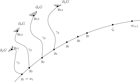
Figure 6. The partition of $\gamma[w_{i},\zeta_{i}]$ and the related quasigeodesic rays.

Moreover, for each $j\in\{2,\ldots,7\}$,

$$\sigma(y_{j},\zeta_{i})\geq\sigma(w_{i},\zeta_{i})-\Sigma_{r=2}^{j}\sigma(y_{r-1},y_{r})\geq\Big{(}1-\frac{j-1}{30}\Big{)}\sigma(w_{i},\zeta_{i}),$$

which implies that for any $p,$ $q\in\{1,\ldots,6\}$,

(6.6) $$\sigma(y_{p},\zeta_{i})\geq 24\sigma(y_{q},y_{q+1}).$$

Since Lemma 6.2 ensures $\delta_{G}(y_{p})\leq 2\delta_{G}(u_{i})$ for each $p\in\{1,\ldots,6\}$, we see from (6.5) that

(6.7) $$k_{G}(y_{p},y_{p+1})\geq\log\frac{\sigma(y_{p},y_{p+1})}{\delta_{G}(y_{p})}>4CC_{1}M\log\frac{M_{1}}{60}.$$

Then, for any $r\in\{1,\ldots,6\}$ and $y\in\gamma[y_{r+1},\zeta_{i}]$,

$$k_{G}(y_{r},y) \geq \frac{1}{M}k_{Y}(y^{\prime}_{r},y^{\prime})\geq\frac{1}{M}k_{Y}(y^{\prime}_{r},y^{\prime}_{r+1})\geq\frac{1}{M^{2}}k_{G}(y_{r},y_{r+1})$$

$$> 4CC_{1}M^{-1}\log\frac{M_{1}}{60}>10,$$

where, in the second inequality, the assumption that $\gamma^{\prime}$ is a quasihyperbolic geodesic in the theorem, is exploited.

Next, we choose points from $\partial_{\sigma}G$ and construct the corresponding quasigeodesic rays by using Lemma 4.8. For each $j\in\{1,\ldots,4\}$, we take $p=j+1$, $q=j$ in (6.6) and $r=j$ in (6). We see that the quadruple $[y_{j},y_{j+1},\zeta_{i}:\gamma[y_{j+1},\zeta_{i}]]$ has Property . Then, it follows from Lemma 4.8 that for each $j\in\{1,\ldots,4\}$, there exist a point $y_{0,j}\in\partial_{\sigma}G$ and a $100$-quasigeodesic ray $\gamma_{j}$ in $G$ from $y_{j}$ to $y_{0,j}$ such that for any $y\in\gamma_{j}$,

(6.9) $$\frac{1}{42}\sigma(y_{j},y_{j+1})\leq\sigma(y_{j+1},y)\leq 5\sigma(y_{j},y_{j+1})\;\;\mbox{and}\;\;\ell(\gamma_{j}[y,y_{0,j}))\leq 5\delta_{G}(y)$$

(see Figure 6).

Now, we establish the upper bound for $k_{Y}(y^{\prime}_{3},\gamma^{\prime}_{4})$ given in (6.13). We shall reach this goal by two steps.

In the first step, we use Lemma 4.10 and Lemma 4.12 to obtain a relationship between $\ell(\gamma^{\prime}_{j})$ and $\delta_{Y}(y^{\prime}_{j+1})$ as stated in (6.11) below. We know from (6.7) and (6.9) that the quadruple $[y_{j+1},y_{j},y_{0,j};\gamma_{j}]$ has Property with $A_{1}=\big{(}\frac{M_{1}}{60}\big{)}^{2CM}$. Then, it follows from Lemma 4.12 that for each $j\in\{1,2,3\}$,

(6.10) $$C\log M_{1}<M^{-1}k_{G}(y_{j+1},\gamma_{j})\leq k_{Y}(y^{\prime}_{j+1},\gamma^{\prime}_{j}),$$

which, along with Lemma 6.3(3) and the fact that all curves $\gamma^{\prime}_{j}$ are $C$-uniform (by Lemma 4.7), shows that the quadruple $[y^{\prime}_{j+1},y^{\prime}_{j},y^{\prime}_{0,j};\gamma^{\prime}_{j}]$ has Property . Thus, we see from Lemma 4.10 that for each $j\in\{1,2\}$,

(6.11) $$\ell(\gamma^{\prime}_{j})\leq M_{2}^{-1}\delta_{Y}(y^{\prime}_{j+1}).$$

In the second step, we show the inequality (6.13) by applying Lemma 4.11. First, let us check that the sextuple $[y^{\prime}_{1},y^{\prime}_{4},y^{\prime}_{3},y^{\prime}_{0,4};\gamma^{\prime}[y^{\prime}_{1},y^{\prime}_{4}],\gamma^{\prime}_{4}]$ has Property . It follows from (6.10), Lemma 4.3(1) and Lemma 6.3(3) that for each $j\in\{1,2,3\}$,

$$C\log M_{1}\leq k_{Y}(y^{\prime}_{j+1},y^{\prime}_{j})\leq 4M^{2}\log\Big{(}1+\frac{C\delta_{Y}(y^{\prime}_{j+1})}{\delta_{Y}(y^{\prime}_{j})}\Big{)},$$

and, therefore,

(6.12) $$\delta_{Y}(y^{\prime}_{j})<M_{2}^{-2}\delta_{Y}(y^{\prime}_{j+1}).$$

Because

$$\sigma(y_{0,1},y_{0,4}) \leq \ell(\gamma_{1})+\ell(\gamma_{4})+\sigma(y_{1},y_{4})$$

$$\leq 5\delta_{G}(y_{1})+5\delta_{G}(y_{4})+\frac{1}{10}\sigma(w_{i},\zeta_{i})\;\;\;(\mbox{by \eqref{MQW-3} and \eqref{MQW-7}})$$

$$< \frac{1}{5}\sigma(w_{i},\zeta_{i}),\;\;\;(\mbox{by \eqref{wed-13} and Lemma \ref{lem-5.1}})$$

and since the similar reasoning as above implies that

$$\sigma(y_{0,1},y_{0,2})\geq\sigma(y_{1},y_{2})-\ell(\gamma_{1})-\ell(\gamma_{2})>\frac{1}{32}\sigma(w_{i},\zeta_{i}),$$

we see from the assumption that $f$ is $\eta$-quasisymmetric on $\partial_{\sigma}G$ of Property that

$$\frac{d^{\prime}(y^{\prime}_{0,1},y^{\prime}_{0,4})}{d^{\prime}(y^{\prime}_{0,1},y^{\prime}_{0,2})}\leq\eta\bigg{(}\frac{\sigma(y_{0,1},y_{0,4})}{\sigma(y_{0,1},y_{0,2})}\bigg{)}<\eta(7).$$

Hence,

$$d^{\prime}(y^{\prime}_{0,1},y^{\prime}_{0,4})<\eta(7)d^{\prime}(y^{\prime}_{0,1},y^{\prime}_{0,2}),$$

and, thus,

$$d^{\prime}(y^{\prime}_{1},y^{\prime}_{0,4}) \leq d^{\prime}(y^{\prime}_{0,1},y^{\prime}_{1})+d^{\prime}(y^{\prime}_{0,1},y^{\prime}_{0,4})<\ell(\gamma^{\prime}_{1})+\eta(7)d^{\prime}(y^{\prime}_{0,1},y^{\prime}_{0,2})$$

$$\leq \ell(\gamma^{\prime}_{1})+\eta(7)\big{(}d^{\prime}(y^{\prime}_{1},y^{\prime}_{2})+\ell(\gamma^{\prime}_{1})+\ell(\gamma^{\prime}_{2})\big{)}$$

$$< 2\eta(7)M_{2}^{-1}\delta_{Y}(y^{\prime}_{3})\;\;\;(\mbox{by (\ref{MQW-10}), (\ref{MQW-11}) and Lemma \ref{lem-5.2}\eqref{lem-5.2(3)}})$$

$$< 3\eta(7)M_{2}^{-1}\min\{d^{\prime}(y^{\prime}_{1},y^{\prime}_{3}),d^{\prime}(y^{\prime}_{1},y^{\prime}_{4}),d^{\prime}(y^{\prime}_{4},y^{\prime}_{0,4})\},$$

where, the last inequality is based on the following estimates: By (6.12), we have

$$d^{\prime}(y^{\prime}_{1},y^{\prime}_{3})\geq\delta_{Y}(y^{\prime}_{3})-\delta_{Y}(y^{\prime}_{1})\geq(1-M_{2}^{-4})\delta_{Y}(y^{\prime}_{3}),$$

$$d^{\prime}(y^{\prime}_{1},y^{\prime}_{4})\geq\delta_{Y}(y^{\prime}_{4})-\delta_{Y}(y^{\prime}_{1})\geq(M_{2}^{2}-M_{2}^{-4})\delta_{Y}(y^{\prime}_{3})$$

and

$$d^{\prime}(y^{\prime}_{4},y^{\prime}_{0,4})\geq\delta_{Y}(y^{\prime}_{4})\geq M_{2}^{2}\delta_{Y}(y^{\prime}_{3}).$$

Then, we see from Lemma 6.3(3), the fact that $\gamma^{\prime}_{4}$ is $C$-uniform (by Lemma 4.7) and the assumption that $\gamma^{\prime}$ is a quasihyperbolic geodesic in the theorem that the sextuple $[y^{\prime}_{1},y^{\prime}_{4},y^{\prime}_{3},y^{\prime}_{0,4};\gamma^{\prime}[y^{\prime}_{1},y^{\prime}_{4}],\gamma^{\prime}_{4}]$ has Property . Hence, we conclude from Lemma 4.11 that

(6.13) $$k_{Y}(y^{\prime}_{3},\gamma^{\prime}_{4})\leq 12M\log C_{1}.$$

It follows from (6.5), (6.9) and Lemma 6.2 that

$$k_{Y}(y^{\prime}_{3},\gamma^{\prime}_{4})\geq M^{-1}k_{G}(y_{3},\gamma_{4})\geq M^{-1}\log\frac{\sigma(y_{3},y_{4})-\ell(\gamma_{4})}{\delta_{G}(y_{3})}>12M\log C_{1},$$

which contradicts (6.13). The proof of Lemma 6.4 is complete.∎

Lemma 6.5.

Suppose there is $i\in\{1,\ldots,\tau\}$ such that $\ell(\gamma[w_{i},w_{i+1}])>A_{0}\delta_{G}(u_{i}).$ If there exist $x$ and $y\in\gamma[w_{i},w_{i+1}]$ such that $\ell(\gamma[x,y])\geq\frac{1}{7}\ell(\gamma[w_{i},w_{i+1}])$, then

$$k_{G}(x,y)>M^{-2}\log\frac{A_{0}}{14}.$$

Proof. By the assumption that $f|_{G}$ is $M$-quasihyperbolic of Property and the assumption that $\gamma^{\prime}$ is a quasihyperbolic geodesic in the theorem, we see from Lemma 4.6 that

$$k_{G}(x,y)\geq M^{-2}\ell_{k_{G}}(\gamma[x,y])\geq M^{-2}\log\frac{\ell(\gamma[x,y])}{\delta_{G}(x)}.$$

Hence, from the assumptions in the lemma and Lemma 6.2, it follows that

$$k_{G}(x,y)>M^{-2}\log\frac{A_{0}}{14},$$

as required. ∎

Lemma 6.6.

Suppose there is $i\in\{1,\ldots,\tau\}$ such that $\ell(\gamma[w_{i},w_{i+1}])>A_{0}\delta_{G}(u_{i}).$ Then, there are consecutive points $z_{1}$, $z_{2}$, $z_{3}$, $z_{4}$ and $z_{5}$ on $\gamma[w_{i},w_{i+1}]$ ordered along the direction from $w_{i}$ to $w_{i+1}$, and $z_{0,1}$, $z_{0,2}$ and $z_{0,5}$ in $\partial_{\sigma}G$ such that (see Figure 7)

1. $\ell(\gamma^{\prime}[z^{\prime}_{1},z^{\prime}])\leq C\delta_{Y}(z^{\prime})$ for any $z^{\prime}\in\gamma^{\prime}[z^{\prime}_{1},w^{\prime}_{i+1}]$;

2. for any $p$, $t\in\{1,2,3,4,5\}$ with $p\not=t$, $k_{G}(z_{p},z_{t})\geq M^{-6}\log\frac{A_{0}}{14}$;

3. for each $q\in\{1,2,5\}$, there exists a $100$-quasigeodesic ray $\beta_{q}$ in $G$ starting from $z_{q}$ and ending at $z_{0,q}$ such that for any $w\in\beta_{q}$,

   $$\ell(\beta_{q}[w,z_{0,q}))\leq 5\delta_{G}(w);$$

4. for each $p\in\{1,2,3,4\},$ $\delta_{Y}(z^{\prime}_{p})<\min\{\big{(}M_{1}\eta(B_{0}^{2})\big{)}^{-1},e^{-B_{0}^{2}}\}\delta_{Y}(z^{\prime}_{p+1}).$

Proof. We start the proof with a partition of the curve $\gamma[w_{i},w_{i+1}]$. Let $v_{j}$ ($j\in\{1,2,\ldots,8\}$) be consecutive points in $\gamma[w_{i},w_{i+1}]$ such that for each $j\in\{1,2,\ldots,7\},$

$$\ell(\gamma[v_{j},v_{j+1}])=\frac{1}{7}\ell(\gamma[w_{i},w_{i+1}]),$$

where $v_{1}=w_{i}$ and $v_{8}=w_{i+1}$ (see Figure 7).

Figure 7. The partition of $\gamma[w_{i},w_{i+1}]$ and the related quasigeodesic rays.

Next, we find the required points and quasigeodesic rays, based on the partition $P_{\gamma[w_{i},w_{i+1}]}=\{v_{j}\}_{j=1}^{8}$.

Claim 6.1.

There exist three points $\mu_{1}\in\gamma[v_{1},v_{2}]$, $\mu_{2}\in\gamma[v_{2},v_{3}]$, $\mu_{0,1}\in\partial_{\sigma}G$ and a $100$-quasigeodesic ray $\beta_{1}$ in $G$ starting from $\mu_{1}$ and ending at $\mu_{0,1}$ such that

1. $k_{G}(\mu_{1},\mu_{2})>M^{-2}\log\frac{A_{0}}{14}$;

2. for any $\mu\in\beta_{1}$, $\ell(\beta_{1}[\mu,\mu_{0,1}))\leq 5\delta_{G}(\mu).$

To find the points $\mu_{1}$ and $\mu_{2}$, we consider two possibilities. If $|v_{1}-v_{2}|\leq|v_{2}-v_{3}|$, then we set $\mu_{1}=v_{1}$ and $\mu_{2}\in\mathbb{S}(v_{2},|v_{1}-v_{2}|)\cap\gamma[v_{2},v_{3}]$ (see Figure 7).

If $|v_{1}-v_{2}|>|v_{2}-v_{3}|$, then we set $\mu_{1}\in\mathbb{S}(v_{2},|v_{2}-v_{3}|)\cap\gamma[v_{1},v_{2}]$ and $\mu_{2}=v_{3}$. Since

$$\ell(\gamma[\mu_{1},\mu_{2}])\geq\frac{1}{7}\ell(\gamma[w_{i},w_{i+1}]),$$

we see from Lemma 6.5 that the first statement in the claim holds. Hence, the quadruple $[\mu_{1},v_{2},\mu_{2};\gamma[v_{2},\mu_{2}]]$ has Property . Thus, it follows from Corollary 4.9 that there exist a point $\mu_{0,1}\in\partial_{\sigma}G$ and a $100$-quasigeodesic ray $\beta_{1}$ in $G$ starting from $\mu_{1}$ and ending at $\mu_{0,1}$ satisfying the second statement of the claim (see Figure 7), proving the claim.

By replacing the triple $(v_{1},v_{2},v_{3})$ with $(\mu_{2},v_{4},v_{5})$ (resp. the one $(v_{6},v_{7},v_{8})$), and using a similar argument as in the proof of Claim 6.1, we see that the following two claims hold:

Claim 6.2.

There exist three points $\mu_{3}\in\gamma[\mu_{2},v_{4}]$, $\mu_{4}\in\gamma[v_{4},v_{5}]$, $\mu_{0,3}\in\partial_{\sigma}G$, and a $100$-quasigeodesic ray $\beta_{2}$ in $G$ starting from $\mu_{3}$ and ending at $\mu_{0,3}$ such that

1. $k_{G}(\mu_{3},\mu_{4})>M^{-2}\log\frac{A_{0}}{14}$;

2. for any $\mu\in\beta_{2}$, $\ell(\beta_{2}[\mu,\mu_{0,3}))\leq 5\delta_{G}(\mu)$ (see Figure 7).

Claim 6.3.

There exist three points $\mu_{5}\in\gamma[v_{6},v_{7}]$, $\mu_{6}\in\gamma[v_{7},v_{8}]$, $\mu_{0,6}\in\partial_{\sigma}G$ and a $100$-quasigeodesic ray $\beta_{5}$ starting from $\mu_{6}$ and ending at $\mu_{0,6}$ in $G$ such that

1. $k_{G}(\mu_{5},\mu_{6})>M^{-2}\log\frac{A_{0}}{14}$;

2. for any $\mu\in\beta_{5}$, $\ell(\beta_{5}[\mu,\mu_{0,6}))\leq 5\delta_{G}(\mu)$ (see Figure 7).

Next, we derive lower bounds for the quasihyperbolic distances between certain pairs of the above constructed points. First, we see that

$$\;\;\;\;\;\;\;\;\;\;\;\;k_{G}(\mu_{3},v_{5}) \geq M^{-1}k_{Y}(\mu^{\prime}_{3},v^{\prime}_{5})\;\;\;(\mbox{since $f|_{G}$ is $M$-quasihyperbolic})$$

$$\geq M^{-1}k_{Y}(\mu^{\prime}_{3},\mu^{\prime}_{4})$$

$$\geq M^{-2}k_{G}(\mu_{3},\mu_{4})\;\;\;(\mbox{since $f|_{G}$ is $M$-quasihyperbolic})$$

$$\geq M^{-4}\log\frac{A_{0}}{14},\;\;\;(\mbox{by Claim \ref{cl-5.2}})$$

where, in the second inequality, the fact that $\mu^{\prime}_{4}\in\gamma^{\prime}[\mu^{\prime}_{3},v_{5}^{\prime}]$ and the assumption in the theorem that $\gamma^{\prime}$ is a quasihyperbolic geodesic, are applied.

Similarly, it follows from Claim 6.1 and Claim 6.2 that for $\mu_{3}\in\gamma[\mu_{2},v_{4}]$,

(6.15) $$k_{G}(\mu_{1},\mu_{3})\geq M^{-1}k_{Y}(\mu^{\prime}_{1},\mu^{\prime}_{3})\geq M^{-2}k_{G}(\mu_{1},\mu_{2})\geq M^{-4}\log\frac{A_{0}}{14},$$

and from Lemma 6.5 that

(6.16) $$k_{G}(v_{5},v_{6})\geq M^{-2}\log\frac{A_{0}}{14}\;\;\mbox{and}\;\;k_{G}(v_{6},\mu_{6})\geq M^{-2}\log\frac{A_{0}}{14},$$

where in the second inequality, the fact that $v_{7}\in\gamma[v_{6},\mu_{6}]$ is exploited.

Now, let $z_{1}=\mu_{1}$, $z_{2}=\mu_{3}$, $z_{3}=v_{5}$, $z_{4}=v_{6}$, $z_{5}=\mu_{6}$, $z_{0,1}=\mu_{0,1}$, $z_{0,2}=\mu_{0,3}$ and $z_{0,5}=\mu_{0,6}$ (see Figure 7). Then, for each $p\in\{1,2,3,4\}$, we see from (6) $\sim$ (6.16) that

(6.17) $$k_{G}(z_{p},z_{p+1})\geq M^{-4}\log\frac{A_{0}}{14},$$

and, so for each pair $p,t\in\{1,2,3,4,5\}$ with $p+1<t$,

$$k_{G}(z_{p},z_{t}) \geq M^{-1}k_{Y}(z^{\prime}_{p},z^{\prime}_{t})\geq M^{-1}k_{Y}(z^{\prime}_{p},z^{\prime}_{p+1})$$

$$\geq M^{-2}k_{G}(z_{p},z_{p+1})\geq M^{-6}\log\frac{A_{0}}{14}.$$

Lemma 6.3(3), (6.17), (6) and Claims 6.1 $\sim$ 6.3 show that the first three statements of the lemma hold.

The last statement in the lemma follows from the following chain of inequalities: For each $p\in\{1,2,3,4\}$,

$$M^{-6}\log\frac{A_{0}}{14} \leq k_{G}(z_{p},z_{p+1})\;\;\;(\mbox{by Lemma \ref{tau-1}\eqref{tau-1(2)}})$$

$$\leq Mk_{Y}(z^{\prime}_{p+1},z^{\prime}_{p})\;\;\;(\mbox{since $f^{-1}|_{Y}$ is also $M$-quasihyperbolic})$$

$$\leq 4M^{3}\log\Big{(}1+\frac{d^{\prime}(z^{\prime}_{p+1},z^{\prime}_{p})}{\min\{\delta_{Y}(z^{\prime}_{p}),\delta_{Y}(z^{\prime}_{p+1})}\Big{)}\;\;\;(\mbox{by Lemma}\;\ref{h-W-1}(1))$$

$$\leq 4M^{3}\log\Big{(}1+\frac{C\delta_{Y}(z^{\prime}_{p+1})}{\delta_{Y}(z^{\prime}_{p})}\Big{)}.\;\;\;(\mbox{by Lemma \ref{lem-5.2}(3)})$$

The proof of the lemma is complete. ∎

Next, we establish more properties of the points and the quasigeodesic rays constructed in Lemma 6.6.

Lemma 6.7.

Under assumptions of Lemma 6.6,

1. $\min\{d^{\prime}(z^{\prime}_{1},z^{\prime}_{4}),d^{\prime}(z^{\prime}_{1},z^{\prime}_{5}),d^{\prime}(z^{\prime}_{0,5},z^{\prime}_{5})\}\geq(1-M_{1}^{-1})\delta_{Y}(z^{\prime}_{4})$, and

2. $\sigma(z_{0,1},z_{0,5})\leq 2M_{1}^{4CC_{1}M}\delta_{G}(u_{i})$.

Proof. By Lemma 6.6(4), we have

$$d^{\prime}(z^{\prime}_{1},z^{\prime}_{5})\geq\delta_{Y}(z^{\prime}_{5})-\delta_{Y}(z^{\prime}_{1})>(e^{B_{0}^{2}}-1)\delta_{Y}(z^{\prime}_{4}),$$

$$d^{\prime}(z^{\prime}_{1},z^{\prime}_{4})\geq\delta_{Y}(z^{\prime}_{4})-\delta_{Y}(z^{\prime}_{1})>(1-M_{1}^{-1})\delta_{Y}(z^{\prime}_{4})$$

and

$$d^{\prime}(z^{\prime}_{0,5},z^{\prime}_{5})\geq\delta_{Y}(z^{\prime}_{5})>(1-M_{1}^{-1})\delta_{Y}(z^{\prime}_{4}).$$

These prove the first statement of the lemma.

Since

$$\sigma(z_{1},z_{5})\leq\sigma(w_{i},z_{1})+\sigma(w_{i},z_{5})\leq 2\sigma(w_{i},\zeta_{i}),$$

we see that

$$\sigma(z_{0,1},z_{0,5}) \leq \ell(\beta_{1})+\ell(\beta_{5})+\sigma(z_{1},z_{5})$$

$$\leq 5\delta_{G}(z_{1})+5\delta_{G}(z_{5})+2\sigma(w_{i},\zeta_{i})\;\;\;(\mbox{by Lemma}\;\ref{tau-1}\eqref{tau-1(3)})$$

$$< 2M_{1}^{4CC_{1}M}\delta_{G}(u_{i}),\;\;\;(\mbox{by Lemmas \ref{lem-5.1} and \ref{MQW-4}})$$

from which the second statement in the lemma follows. ∎

Lemma 6.8.

Under assumptions of Lemma 6.6, the following statements hold: For $p\in\{1,2,\ldots,5\}$ and $q\in\{1,2,5\}$,

1. if $p\not=q$, then $\sigma(z_{p},\beta_{q})>\frac{1}{4}B_{0}^{-1}M_{0}^{-1}\sigma(z_{p},z_{q});$

2. if $p\not=q$, then $k_{Y}(z^{\prime}_{p},\beta^{\prime}_{q})\geq\frac{1}{3}C_{1}^{-1}M^{-7}\log A_{0},$ and

3. if $p=q+1$ and $q=1$ or $2$, then $\ell(\beta^{\prime}_{q})\leq M_{2}^{-1}\delta_{Y}(z^{\prime}_{p})$.

Proof. For the proof of the first statement in the lemma, we let $z\in\beta_{q}$. We divide the argument into two cases. For the first case $\ell(\beta_{q}[z,z_{0,q}))\leq\frac{1}{50}B_{0}^{-1}\ell(\beta_{q})$, we see that

$$\sigma(z_{p},z) \geq \delta_{G}(z_{p})-\delta_{G}(z)\geq\delta_{G}(z_{p})-\frac{1}{50}B_{0}^{-1}\ell(\beta_{q})$$

$$\geq \delta_{G}(z_{p})-\frac{1}{10}B_{0}^{-1}\delta_{G}(z_{q})\;\;\;(\mbox{by Lemma}\;\ref{tau-1}\eqref{tau-1(3)})$$

$$> \frac{1}{4}B_{0}^{-1}\delta_{G}(u_{i})>\frac{1}{2}B_{0}^{-1}M_{0}^{-1}\sigma(w_{i},\zeta_{i})\;\;\;(\mbox{by Lemmas \ref{lem-5.1} and \ref{MQW-4}})$$

$$\geq \frac{1}{4}B_{0}^{-1}M_{0}^{-1}\sigma(z_{p},z_{q}).\;\;\;(\mbox{by \eqref{WWW-1}})$$

For the remaining case, $\ell(\beta_{q}[z,z_{0,q}))>\frac{1}{50}B_{0}^{-1}\ell(\beta_{q})$, we observe that

$$k_{G}(z,z_{q}) \leq 20\log\Big{(}1+\frac{\ell(\beta_{q}[z,z_{q}])}{\delta_{G}(z)}\Big{)}\;\;\;(\mbox{by Lemmas \ref{H-W-Zhou-0} and \ref{tau-1}\eqref{tau-1(3)}})$$

$$\leq 20\log\Big{(}1+\frac{5\ell(\beta_{q})}{\ell(\beta_{q}[z,z_{0,q}))}\Big{)}\;\;\;(\mbox{by Lemma \ref{tau-1}\eqref{tau-1(3)}})$$

$$< 30\log B_{0},$$

and, thus, Lemma 6.6(2) implies

$$k_{G}(z_{p},z)\geq k_{G}(z_{q},z_{p})-k_{G}(z,z_{q})>\frac{1}{2}M^{-6}\log\frac{A_{0}}{14},$$

which, together with Lemma 4.1, guarantees that $|z_{p}-z|>\frac{1}{2}\delta_{G}(z_{p})$. Moreover, from Lemmas 6.2 and 6.4, we obtain

$$\sigma(z_{p},z) \geq |z_{p}-z|>\frac{1}{2}\delta_{G}(z_{p})\geq\frac{1}{4}B_{0}^{-1}\delta_{G}(u_{i})\;\;\;(\mbox{by Lemma \ref{lem-5.1}})$$

$$> \frac{1}{4}B_{0}^{-1}M_{0}^{-1}\sigma(z_{p},z_{q}).\;\;\;(\mbox{by Lemma \ref{MQW-4}})$$

Hence, the first statement in the lemma is true.

For $p\in\{1,2,3,4,5\}$ and $q\in\{1,2,5\}$ with $p\not=q$, Lemma 6.6(2), Lemma 6.6(3) and the first statement in the lemma imply that the quadruple $[z_{p},z_{q},z_{0,q};\beta_{q}]$ has Property with $A_{1}=\big{(}\frac{A_{0}}{14}\big{)}^{\frac{1}{2}c_{1}^{-1}M^{-6}}$. Then, Lemma 4.12 yields

$$k_{Y}(z^{\prime}_{p},\beta^{\prime}_{q})\geq M^{-1}k_{G}(z_{p},\beta_{q})\geq\frac{1}{2}C_{1}^{-1}M^{-7}\log\frac{A_{0}}{14}-\log 5>\frac{1}{3}C_{1}^{-1}M^{-7}\log A_{0},$$

which shows that the second statement of the lemma.

For each $q\in\{1,2\}$, since $\beta^{\prime}_{q}$ is $C$-uniform (by Lemma 4.7), we see from Lemma 6.6(1) and Lemma 6.8(2) that the quadruple $[z^{\prime}_{q+1},z^{\prime}_{q},z^{\prime}_{0,q};\beta^{\prime}_{q}]$ has Property . Then, it follows from Lemma 4.10 that for each $q\in\{1,2\},$

$$\ell(\beta^{\prime}_{q})\leq M_{2}^{-1}\delta_{Y}(z^{\prime}_{q+1}).$$

Hence, the final statement in the lemma holds, and, so the lemma is proved.∎

The following lemma plays a key role in the proof of Theorem 6.1.

Lemma 6.9.

For each $i\in\{1,\ldots,\tau\}$, we have $\ell(\gamma[u_{i},u_{i+1}])\leq 2A_{0}\delta_{G}(u_{i})$.

Proof. We prove the lemma by contradiction. Assume, to the contrary, that there is $i\in\{1,\ldots,\tau\}$ such that

$$\ell(\gamma[u_{i},u_{i+1}])>2A_{0}\delta_{G}(u_{i}).$$

Then, Lemma 6.3 implies that there are points $w_{i}$ and $w_{i+1}\in\gamma[u_{i},u_{i+1}]$ such that

$$\ell(\gamma[w_{i},w_{i+1}])>A_{0}\delta_{G}(u_{i}).$$

Hence, there are consecutive points $z_{1}$, $z_{2}$, $z_{3}$, $z_{4}$ and $z_{5}$ on $\gamma[w_{i},w_{i+1}]$ ordered along the direction from $w_{i}$ to $w_{i+1}$, points $z_{0,q}$ ($q\in\{1,2,5\}$) in $\partial_{\sigma}G$ and $100$-quasigeodesic rays $\beta_{q}$ in $G$ starting from $z_{q}$ and ending at $z_{0,q}$ satisfying the conditions (1) $\sim$ (4) of Lemma 6.6. Therefore, the claims of Lemma 6.7 and Lemma 6.8 are valid for these points and quasigeodesic rays. To reach a contradiction, we consider two cases.

Case 6.1.

Let $\sigma(z_{0,1},z_{0,2})\geq\frac{1}{100}B_{0}^{-1}\delta_{G}(u_{i}).$

We obtain a contradiction by applying Lemma 4.11. We need to verify that the sextuple $[z^{\prime}_{1},z^{\prime}_{5},z^{\prime}_{4},z^{\prime}_{0,5};\gamma^{\prime}[z^{\prime}_{1},z^{\prime}_{5}],\beta^{\prime}_{5}]$ has Property .

Firstly, we conclude from Lemma 6.6(1) that

$$d^{\prime}(z^{\prime}_{1},z^{\prime}_{2})\leq C\delta_{Y}(z^{\prime}_{2}),$$

and, so we get

$$d^{\prime}(z^{\prime}_{0,1},z^{\prime}_{0,2}) \leq d^{\prime}(z^{\prime}_{1},z^{\prime}_{2})+\ell(\beta^{\prime}_{1})+\ell(\beta^{\prime}_{2})$$

$$\leq C\delta_{Y}(z^{\prime}_{2})+M_{2}^{-1}(\delta_{Y}(z^{\prime}_{2})+\delta_{Y}(z^{\prime}_{3}))\;\;\;(\mbox{by Lemma \ref{cl-thu-1}\eqref{cl-thu-1(3)}})$$

$$< 2M_{1}^{-1}M_{2}^{-1}(\eta(B_{0}^{2}))^{-1}\delta_{Y}(z^{\prime}_{4}).\;\;\;(\mbox{by Lemma \ref{tau-1}\eqref{tau-1(4)}})$$

Secondly, by the assumption that $f$ is $\eta$-quasisymmetric on $\partial_{\sigma}G$ of Property , Lemma 6.7(2) and the assumption of this case, we have

$$\frac{d^{\prime}(z^{\prime}_{0,1},z^{\prime}_{0,5})}{d^{\prime}(z^{\prime}_{0,1},z^{\prime}_{0,2})}\leq\eta\bigg{(}\frac{\sigma(z_{0,1},z_{0,5})}{\sigma(z_{0,1},z_{0,2})}\bigg{)}<\eta(B_{0}M_{0}).$$

Hence,

$$d^{\prime}(z^{\prime}_{0,1},z^{\prime}_{0,5})<\eta(B_{0}M_{0})d^{\prime}(z^{\prime}_{0,1},z^{\prime}_{0,2})<M_{1}^{-1}\delta_{Y}(z^{\prime}_{4}),$$

and, thus, it follows that

$$d^{\prime}(z^{\prime}_{1},z^{\prime}_{0,5}) \leq d^{\prime}(z^{\prime}_{1},z^{\prime}_{0,1})+d^{\prime}(z^{\prime}_{0,1},z^{\prime}_{0,5})$$

$$\leq M_{2}^{-1}\delta_{Y}(z^{\prime}_{2})+M_{1}^{-1}\delta_{Y}(z^{\prime}_{4})\;\;\;(\mbox{by Lemma \ref{cl-thu-1}\eqref{cl-thu-1(3)}})$$

$$< 2M_{1}^{-1}\delta_{Y}(z^{\prime}_{4})\;\;\;(\mbox{by Lemma \ref{tau-1}\eqref{tau-1(4)}})$$

$$< 3M_{1}^{-1}\min\{d^{\prime}(z^{\prime}_{1},z^{\prime}_{5}),d^{\prime}(z^{\prime}_{1},z^{\prime}_{4}),d^{\prime}(z^{\prime}_{5},z^{\prime}_{0,5})\},$$

where in the last inequality, Lemma 6.7(1) is exploited.

Now, we apply Lemma 4.11. From (6), Lemma 6.6(1), the fact that $\beta^{\prime}_{5}$ is $C$-uniform (by Lemma 4.7) and the assumption of the theorem that $\gamma^{\prime}$ is a quasihyperbolic geodesic, we see that the sextuple $[z^{\prime}_{1},z^{\prime}_{5},z^{\prime}_{4},z^{\prime}_{0,5};\gamma^{\prime}[z^{\prime}_{1},z^{\prime}_{5}],\beta^{\prime}_{5}]$ has Property . Then, it follows from Lemma 4.11 that

$$k_{Y}(z^{\prime}_{4},\beta^{\prime}_{5})\leq 12M\log C_{1},$$

which contradicts Lemma 6.8(2). Hence, the lemma is proved in this case.

Case 6.2.

Let $\sigma(z_{0,1},z_{0,2})<\frac{1}{100}B_{0}^{-1}\delta_{G}(u_{i}).$

Under this assumption, we obtain a contradiction by applying Lemma 4.11. First, we need to find two points from the sphere $\mathbb{S}(z_{0,1},r)$, one point from $\partial_{\sigma}G$ and a ray, i.e., $z_{1,1}$, $z^{*}$, $z_{0,0}$ and $\alpha_{1}$ below (see Figure 8), where $r=\frac{1}{6}\min\{\ell(\beta_{1}),\ell(\beta_{2})\}.$

It follows from Lemma 6.2 and Lemma 6.6(3) that

(6.20) $$\frac{1}{12}B_{0}^{-1}\delta_{G}(u_{i})\leq\frac{1}{6}\min\{\delta_{G}(z_{1}),\delta_{G}(z_{2})\}\leq r\leq\frac{5}{6}\min\{\delta_{G}(z_{1}),\delta_{G}(z_{2})\}.$$

Then, Lemma 6.2 and the assumption of this case guarantee that

$$|z_{1}-z_{0,1}|\geq\delta_{G}(z_{1})\geq\frac{6}{5}r,\;\;|z_{0,1}-z_{0,2}|\leq\sigma(z_{0,1},z_{0,2})<\frac{3}{25}r$$

and

$$|z_{2}-z_{0,1}|\geq|z_{2}-z_{0,2}|-\sigma(z_{0,1},z_{0,2})\geq\frac{49}{50}\delta_{G}(z_{2})\geq\frac{147}{125}r.$$

These imply that $\beta_{1}\cap\mathbb{S}(z_{0,1},r)\not=\emptyset$ and $\beta_{2}\cap\mathbb{S}(z_{0,1},r)\not=\emptyset$. Let

$$z_{1,1}\in\beta_{1}\cap\mathbb{S}(z_{0,1},r)\;\;\mbox{and}\;\;z_{1,2}\in\beta_{2}\cap\mathbb{S}(z_{0,1},r)$$

(see Figure 8). Thus, Lemma 6.6(3) ensures that for $q\in\{1,2\}$,

$$|z_{1,q}-z_{0,q}|\leq 5\delta_{G}(z_{1,q}),$$

and, therefore, (6.20) leads to

(6.21) $$\frac{1}{12}B_{0}^{-1}\delta_{G}(u_{i})\leq r\leq 5\delta_{G}(z_{1,1}).$$

The assumption of this case leads to

(6.22) $$\frac{1}{14}B_{0}^{-1}\delta_{G}(u_{i})<r-|z_{0,1}-z_{0,2}|\leq|z_{1,2}-z_{0,2}|\leq 5\delta_{G}(z_{1,2}).$$

Figure 8. The related points and quasigeodesic rays.

For each $q\in\{1,2\}$, it follows from Lemma 4.2 and Lemma 6.6(3) that

$$k_{G}(z_{q},z_{1,{q}})\leq 20\log\Big{(}1+\frac{\ell(\beta_{q}[z_{1,{q}},z_{q}])}{\delta_{G}(z_{1,{q}})}\Big{)}.$$

Therefore, (6.21), (6.22) and Lemma 6.6(3) guarantee that

$$\frac{\ell(\beta_{q}[z_{1,{q}},z_{q}])}{\delta_{G}(z_{1,{q}})}\leq 350B_{0}\frac{\delta_{G}(z_{q})}{\delta_{G}(u_{i})},$$

and we may conclude from Lemma 6.2 that

(6.23) $$k_{G}(z_{q},z_{1,{q}})\leq 20\log(1+700B_{0})<40\log B_{0}.$$

Then, Lemma 6.6(2) yields

(6.24) $$k_{G}(z_{1,1},z_{1,2})\geq k_{G}(z_{1},z_{2})-k_{G}(z_{1},z_{1,1})-k_{G}(z_{2},z_{1,2})>\frac{1}{2}M^{-6}\log A_{0}.$$

By using the points $z_{1,1}$ and $z_{1,2}$, we may find the required two points $z^{*}$, $z_{0,0}$ and the ray $\alpha_{1}$ in the following way. Let $L$ denote the circle in $\mathbb{S}(z_{0,1},r)$ determined by $z_{1,1}$, $z_{1,2}$ and $z_{0,1}$. Now, $L$ is divided into two parts by $z_{1,1}$ and $z_{1,2}$. We denote by $L_{z_{1,1}z_{1,2}}$ the shorter one.

Claim 6.4.

There exists a point $z^{*}\in L_{z_{1,1}z_{1,2}}$ such that

1. $\delta_{G}(z^{*})=\frac{1}{96}B_{0}^{-1}\ell(\beta_{1}[z_{1,1},z_{0,1})),$ and

2. for all $z\in L_{z_{1,1}z^{*}}$, $\delta_{G}(z)>\frac{1}{96}B_{0}^{-1}\ell(\beta_{1}[z_{1,1},z_{0,1}))$ (see Figure 8).

Since Lemma 6.6(3) implies that $\delta_{G}(z_{1,1})\geq\frac{1}{5}\ell(\beta_{1}[z_{1,1},z_{0,1}))$, it suffices to show that there is a point $z\in L_{z_{1,1}z_{1,2}}$ such that

$$\delta_{G}(z)=\frac{1}{96}B_{0}^{-1}\ell(\beta_{1}[z_{1,1},z_{0,1})).$$

This assertion holds because, otherwise, it would follow that

$$k_{G}(z_{1,1},z_{1,2})\leq\int_{L_{z_{1,1}z_{1,2}}}\frac{|dz|}{\delta_{G}(z)}\leq 96\pi B_{0},$$

which contradicts (6.24).

By Claim 6.4, we see from Lemma 6.2 and Lemma 6.6(3) that

(6.25) $$k_{G}(z_{1,1},z^{*})\leq 96\pi B_{0}\;\;\mbox{and}\;\;\delta_{G}(z^{*})\leq\frac{5}{48}B_{0}^{-1}\delta_{G}(u_{i}).$$

Take $z_{0,0}\in\partial_{\sigma}G$ with

(6.26) $$\delta_{G}(z^{*})=|z^{*}-z_{0,0}|,$$

and let

$$\alpha_{1}=[z^{*},z_{0,0})$$

(see Figure 8). Then, $\alpha^{\prime}_{1}$ is $C$-uniform (by the assumption that $f|_{G}$ is $M$-quasihyperbolic and Lemma 4.7).

Now, we verify that the sextuple $[z^{\prime}_{1},z^{\prime}_{5},z^{\prime}_{4},z^{\prime}_{0,5};\gamma^{\prime}[z^{\prime}_{1},z^{\prime}_{5}],\beta^{\prime}_{5}]$ has Property . We shall reach this goal by three steps.

In the first step, we utilize Lemma 4.12 to get a lower bound for the quantity $k_{Y}(z^{\prime}_{2},\alpha^{\prime}_{1})$. Since Lemma 6.2 and (6.25) lead to

$$\sigma(z_{2},z^{*})\geq\delta_{G}(z_{2})-\delta_{G}(z^{*})\geq\frac{19}{5}\delta_{G}(z^{*}),$$

we see that for any $z\in\alpha_{1}$,

(6.27) $$\sigma(z_{2},z)\geq\sigma(z_{2},z^{*})-\sigma(z^{*},z)\geq\frac{14}{19}\sigma(z_{2},z^{*}).$$

Furthermore, (6.23), (6.25) and Lemma 6.6(2) lead to

$$k_{G}(z_{2},z^{*})\geq k_{G}(z_{1},z_{2})-k_{G}(z_{1},z_{1,1})-k_{G}(z_{1,1},z^{*})>\frac{1}{2}M^{-6}\log A_{0},$$

and, thus, (6.27) implies that quadruple $[z_{2},z^{*},z_{0,0};\alpha_{1}]$ has Property with $A_{1}=A_{0}^{\frac{1}{4}C_{1}^{-1}M^{-6}}$. Then, Lemma 4.12 shows the following:

(6.28) $$k_{Y}(z^{\prime}_{2},\alpha^{\prime}_{1})\geq M^{-1}k_{G}(z_{2},\alpha_{1})>\frac{1}{8}C_{1}^{-1}M^{-7}\log A_{0}.$$

In the second step, we use Lemma 4.10 to establish a relationship between $\ell(\alpha^{\prime}_{1})$ and $\delta_{Y}(z^{\prime}_{2}).$ Since

$$\max\bigg{\{}\log\frac{d^{\prime}(z^{\prime}_{1},{z^{*}}^{\prime})}{\delta_{Y}(z^{\prime}_{1})},\log\frac{\delta_{Y}({z^{*}}^{\prime})}{\delta_{Y}(z^{\prime}_{1})}\bigg{\}} \leq k_{Y}(z^{\prime}_{1},{z^{*}}^{\prime})$$

$$\leq Mk_{G}(z_{1},z^{*})\;\;\;(\mbox{$f|_{G}$ is $M$-quasihyperbolic})$$

$$\leq M(k_{G}(z_{1},z_{1,1})+k_{G}(z_{1,1},z^{*}))$$

$$< 97\pi MB_{0},\;\;\;(\mbox{by (\ref{sat-9}) and (\ref{MQW-30})})$$

we obtain

(6.29) $$\max\{\delta_{Y}({z^{*}}^{\prime}),d^{\prime}(z^{\prime}_{1},{z^{*}}^{\prime})\}<e^{97\pi MB_{0}}\delta_{Y}(z^{\prime}_{1}).$$

Then, we see from Lemma 6.6(1) and Lemma 6.6(4) that

$$d^{\prime}(z^{\prime}_{2},{z^{*}}^{\prime})\leq d^{\prime}(z^{\prime}_{1},{z^{*}}^{\prime})+d^{\prime}(z^{\prime}_{1},z^{\prime}_{2})\leq e^{97\pi MB_{0}}\delta_{Y}(z^{\prime}_{1})+C\delta_{Y}(z^{\prime}_{2})<2C\delta_{Y}(z^{\prime}_{2}),$$

which, together with (6.28) and the fact that $\alpha^{\prime}_{1}$ is $C$-uniform, shows that the quadruple $[z^{\prime}_{2},{z^{*}}^{\prime},z^{\prime}_{0,0};\alpha^{\prime}_{1}]$ has Property . Therefore, Lemma 4.10 implies

(6.30) $$\ell(\alpha^{\prime}_{1})\leq M_{2}^{-1}\delta_{Y}(z^{\prime}_{2}).$$

As the last step, we check that the sextuple $[z^{\prime}_{1},z^{\prime}_{5},z^{\prime}_{4},z^{\prime}_{0,5};\gamma^{\prime}[z^{\prime}_{1},z^{\prime}_{5}],\beta^{\prime}_{5}]$ has Property . It follows from Lemma 6.6(1), together with the fact that $\beta^{\prime}_{5}$ is $C$-uniform and the assumption of the theorem that $\gamma^{\prime}$ is a quasihyperbolic geodesic, that we only need to verify the validity of the statements (1) and (3) of Property .

First, we have

$$d^{\prime}(z^{\prime}_{0,1},z^{\prime}_{0,0}) \leq d^{\prime}(z^{\prime}_{1},z^{\prime}_{0,1})+d^{\prime}(z^{\prime}_{1},{z^{*}}^{\prime})+d^{\prime}(z^{\prime}_{0,0},{z^{*}}^{\prime})$$

$$< \ell(\beta^{\prime}_{1})+e^{97\pi MB_{0}}\delta_{Y}(z^{\prime}_{1})+M_{2}^{-1}\delta_{Y}(z^{\prime}_{2})\;\;\;(\mbox{by (\ref{MQW-33}) and \eqref{sat-10}})$$

$$< 3M_{2}^{-1}\delta_{Y}(z^{\prime}_{2}).\;\;\;(\mbox{by Lemmas \ref{tau-1}\eqref{tau-1(4)} and \ref{cl-thu-1}\eqref{cl-thu-1(3)}})$$

Furthermore, we need the following upper bound for the ratio $\sigma(z_{0,1},z_{0,5})/\sigma(z_{0,1},z_{0,0})$:

$$\sigma(z_{0,1},z_{0,0}) \geq \sigma(z^{*},z_{0,1})-\sigma(z^{*},z_{0,0})\geq\delta_{G}(z_{1,1})-\delta_{G}(z^{*})\;\;\;(\mbox{by \eqref{changsha-10}})$$

$$> \frac{1}{6}\ell(\beta_{1}[z_{1,1},z_{0,1}))\;\;\;(\mbox{by Lemma \ref{tau-1}\eqref{tau-1(3)} and Claim \ref{changsha-9}\eqref{changsha-9(1)}})$$

$$\geq \frac{1}{144}B_{0}^{-1}M_{1}^{-4CC_{1}M}\sigma(z_{0,1},z_{0,5}).\;\;\;(\mbox{by (\ref{MQW-26}) and Lemma \ref{fri-8}\eqref{fri-8(2)}})$$

By applying the assumption of Property that $f$ is $\eta$-quasisymmetric on $\partial_{\sigma}G$, we observe that

$$\frac{d^{\prime}(z^{\prime}_{0,1},z^{\prime}_{0,5})}{d^{\prime}(z^{\prime}_{0,1},z^{\prime}_{0,0})}\leq\eta\bigg{(}\frac{\sigma(z_{0,1},z_{0,5})}{\sigma(z_{0,1},z_{0,0})}\bigg{)}<\eta(B_{0}M_{0}),$$

and, so

$$d^{\prime}(z^{\prime}_{0,1},z^{\prime}_{0,5})<\eta(B_{0}M_{0})d^{\prime}(z^{\prime}_{0,1},z^{\prime}_{0,0})\leq 3\eta(B_{0}M_{0})M_{2}^{-1}\delta_{Y}(z^{\prime}_{2}).$$

Hence,

$$d^{\prime}(z^{\prime}_{1},z^{\prime}_{0,5}) \leq d^{\prime}(z^{\prime}_{1},z^{\prime}_{0,1})+d^{\prime}(z^{\prime}_{0,1},z^{\prime}_{0,5})$$

$$< (1-M_{1}^{-1})M_{1}^{-1}M_{2}^{-1}\delta_{Y}(z^{\prime}_{4})\;\;(\mbox{by Lemmas \ref{cl-thu-1}\eqref{cl-thu-1(3)} and \ref{tau-1}\eqref{tau-1(4)}})$$

$$< M_{1}^{-1}M_{2}^{-1}\min\{d^{\prime}(z^{\prime}_{1},z^{\prime}_{4}),d^{\prime}(z^{\prime}_{1},z^{\prime}_{5}),d^{\prime}(z^{\prime}_{0,5},z^{\prime}_{5})\},$$

where the last inequality follows from Lemma 6.7(1). This shows that the statements (1) and (3) of Property hold.

Now, we deduce from Lemma 4.11 that

$$k_{Y}(z^{\prime}_{4},\beta^{\prime}_{5})\leq 12M\log C_{1}.$$

Again, this contradicts Lemma 6.8(2), and, thus, the proof of the lemma is complete. ∎

6.1. Proof of Theorem 6.1

Now, we are ready to finish the proof of the theorem. For any $x\in\gamma[x_{1},u_{0}]$, there exists $i\in\{1,\ldots,\tau\}$ such that $x\in\gamma[u_{i},u_{i+1}]$. Thus, we see from (6.1), Lemma 6.2 and Lemma 6.9 that

$$\ell(\gamma[x_{1},x])\leq\sum_{j=1}^{i}\ell(\gamma[u_{j},u_{j+1}])\leq 2A_{0}\sum_{j=1}^{i}\delta_{G}(u_{j})\leq 8A_{0}B_{0}\delta_{G}(x).$$

Hence, the theorem is proved. ∎

Remark 6.10.

It is worth of mentioning that the coefficient $8A_{0}B_{0}$ of the cigar condition in Theorem 6.1 is independent of the dimension $n$ of the space.

7. Inner uniformity under Property

The purpose of this section is to finish the proof of Theorem 1.2. From Theorem 3.2, we see that, it suffices to verify the implication from (3) to (1) in Theorem 1.2. Actually, this implication follows from the following result:

Theorem 7.1.

Suppose the triple $[(\overline{G_{\sigma}},\sigma),(\overline{Y_{d^{\prime}}},d^{\prime});f]$ has Property . Then, $G$ is $32A_{0}B_{0}^{2}$-inner uniform.

Proof. Let $x_{1}$, $x_{2}$ be any two points in $G$. It follows from the uniformity of $(Y,d^{\prime})$ of Property and [14, Proposition 2.8] that there is a quasihyperbolic geodesic $\gamma^{\prime}$ in $Y$ connecting $x^{\prime}_{1}$ and $x^{\prime}_{2}$.

To prove the theorem, it suffices to verify the inner uniformity of $\gamma$, which is the preimage of $\gamma^{\prime}$ with respect to $f$. Furthermore, it follows from Theorem 6.1 that we only need to show that $\gamma$ satisfies the following turning condition with respect to the inner metric:

(7.1) $$\ell(\gamma)\leq 32A_{0}B_{0}^{2}\sigma(x_{1},x_{2}).$$

We divide the proof of (7.1) into two cases. In the first case when there exists a point $w_{0}\in\gamma$ such that

$$\delta_{G}(w_{0})>2\max\{\sigma(x_{1},w_{0}),\sigma(x_{2},w_{0})\},$$

the proof is direct and easy (see Lemma 7.2 and its proof below). In the remaining case, i.e., for all $x\in\gamma$,

$$\delta_{G}(x)\leq 2\max\{\sigma(x_{1},x),\sigma(x_{2},x)\},$$

we prove (7.1) by two steps. In the first step, we obtain an upper bound on the diameter of $\gamma$ in terms of the inner distance between $x_{1}$ and $x_{2}$, which is stated in Lemma 7.3 below. In the second step, based on the upper bound of Lemma 7.3, we show the inequality (7.1) (see also Lemma 7.4 below).

Lemma 7.2.

If there exists a point $w_{0}\in\gamma$ such that

$$\delta_{G}(w_{0})>2\max\{\sigma(x_{1},w_{0}),\sigma(x_{2},w_{0})\},$$

then

$$\ell(\gamma)<3e^{2M^{2}}M^{2}\sigma(x_{1},x_{2}).$$

Proof. Since the assumption in the lemma ensures that the segment $[x_{1},x_{2}]\subset\mathbb{B}(w_{0},\frac{1}{2}\delta_{G}(w_{0}))$, we see that for any $x\in[x_{1},x_{2}]$,

$$\frac{3}{2}\delta_{G}(w_{0})\geq\delta_{G}(w_{0})+|x-w_{0}|\geq\delta_{G}(x)\geq\frac{1}{2}\delta_{G}(w_{0})\geq\frac{1}{2}|x_{1}-x_{2}|,$$

which implies

$$\log\Big{(}1+\frac{\ell(\gamma)}{\delta_{G}(x_{1})}\Big{)} \leq \ell_{k_{G}}(\gamma)\leq M^{2}k_{G}(x_{1},x_{2})\;\;\;(\mbox{by \eqref{vai-lem3.2} and Lemma \ref{H-W-1}})$$

$$\leq M^{2}\int_{[x_{1},x_{2}]}\frac{|dx|}{\delta_{G}(x)}\leq 2M^{2}\frac{\sigma(x_{1},x_{2})}{\delta_{G}(w_{0})}<2M^{2}.$$

Thus,

$$e^{-2M^{2}}\frac{\ell(\gamma)}{\delta_{G}(x_{1})}\leq\log\Big{(}1+\frac{\ell(\gamma)}{\delta_{G}(x_{1})}\Big{)}<2M^{2}\frac{\sigma(x_{1},x_{2})}{\delta_{G}(w_{0})},$$

and, so

$$\ell(\gamma)<3e^{2M^{2}}M^{2}\sigma(x_{1},x_{2}),$$

as required. ∎

Lemma 7.3.

Suppose for any $x\in\gamma$, $\delta_{G}(x)\leq 2\max\{\sigma(x_{1},x),\sigma(x_{2},x)\}.$ Then,

$${\operatorname{diam}}(\gamma)<B_{0}\sigma(x_{1},x_{2}).$$

Proof. It follows from the assumption of the lemma that

(7.2) $$\max\{\delta_{G}(x_{1}),\delta_{G}(x_{2})\}\leq 2\sigma(x_{1},x_{2}).$$

Let $x_{1,1}$, $x_{1,2}\in\partial_{\sigma}G$ be such that

$$\delta_{G}(x_{1})=|x_{1}-x_{1,1}|,\;\;\delta_{G}(x_{2})=|x_{2}-x_{1,2}|$$

and

(7.3) $$\gamma_{1,1}=[x_{1},x_{1,1}),\;\;\gamma_{1,2}=[x_{2},x_{1,2})$$

(see Figure 9).

Figure 9. The related points and curves.

We prove the lemma by contradiction. Assume, to the contrary, that

(7.4) $${\operatorname{diam}}(\gamma)\geq B_{0}\sigma(x_{1},x_{2}).$$

Let $z_{0}\in\gamma$ be such that

$$\sigma(x_{1},z_{0})=\frac{1}{2}{\operatorname{diam}}(\gamma)$$

(see Figure 9). Then,

$$\sigma(x_{1},x_{2})\leq 2B_{0}^{-1}\sigma(x_{1},z_{0}),$$

which implies

(7.5) $$\min\{\sigma(x_{1},z_{0}),\sigma(x_{2},z_{0})\}\geq\max\{\frac{2}{3}\sigma(x_{1},z_{0}),\frac{1}{3}B_{0}\sigma(x_{1},x_{2})\},$$

and, thus, (7.2) shows that

(7.6) $$\max\{\delta_{G}(x_{1}),\delta_{G}(x_{2})\}\leq 6B_{0}^{-1}\min\{\sigma(x_{1},z_{0}),\sigma(x_{2},z_{0})\}.$$

Next, we prove two claims.

Claim 7.1.

Suppose there are $i\in\{1,2\}$ and a point $u\in\gamma$ such that $\sigma(x_{i},u)\geq 6B_{0}^{-1}\sigma(x_{1},z_{0})$. Then,

$$\delta_{G}(u)\leq 2\sigma(x_{i},u).$$

By (7.6), we have

$$\delta_{G}(u)\leq\delta_{G}(x_{i})+\sigma(x_{i},u)\leq 6B_{0}^{-1}\sigma(x_{1},z_{0})+\sigma(x_{i},u)\leq 2\sigma(x_{i},u),$$

which is the required estimate.

Claim 7.2.

Suppose there are $i\in\{1,2\}$ and a point $v_{i}\in\gamma[x_{i},z_{0}]$ such that

$$\min\{\sigma(x_{i},v_{i}),\sigma(x_{i+1},v_{i})\}\leq M_{1}^{-\frac{1}{4}}\sigma(x_{1},z_{0}),$$

where $x_{i+1}=x_{1}$ when $i=2$. Then, for all $v\in\gamma[x_{i+1},z_{0}]$,

$$k_{G}(v_{i},v)\geq\frac{1}{4}M^{-2}\log M_{1}-1.$$

First, we prove the following inequality:

(7.7) $$\sigma(x_{i},v_{i})\leq 2M_{1}^{-\frac{1}{4}}\sigma(x_{1},z_{0}).$$

For the case $\min\{\sigma(x_{i},v_{i}),\sigma(x_{i+1},v_{i})\}=\sigma(x_{i},v_{i})$, the inequality is obvious. For the remaining case, $\min\{\sigma(x_{i},v_{i}),\sigma(x_{i+1},v_{i})\}=\sigma(x_{i+1},v_{i})$, we have

$$\sigma(x_{i},v_{i})\leq\sigma(x_{i+1},v_{i})+\sigma(x_{1},x_{2})\leq 2M_{1}^{-\frac{1}{4}}\sigma(x_{1},z_{0}),\;\;\;\mbox{(by \eqref{Corr-12-Tues-2})}$$

as required.

Now, it follows that

$$\sigma(x_{i},z_{0})-\sigma(x_{i},v_{i})\geq\big{(}\frac{2}{3}-2M_{1}^{-\frac{1}{4}}\big{)}\sigma(x_{1},z_{0})\;\;\;\mbox{(by \eqref{Corr-12-Tues-2} and \eqref{shantou-3})}$$

and

$$\sigma(x_{i},v_{i})+\delta_{G}(x_{i})\leq(6B_{0}^{-1}+2M_{1}^{-\frac{1}{4}}\big{)}\sigma(x_{1},z_{0}).\;\;\;\mbox{(by \eqref{changsha-12} and \eqref{shantou-3})}$$

These guarantee that

$$k_{G}(v_{i},v) \geq M^{-2}\ell_{k_{G}}(\gamma[v_{i},v])\;\;\;(\mbox{by Lemma \ref{H-W-1}})$$

$$\geq M^{-2}k_{G}(v_{i},z_{0})\geq M^{-2}\log\Big{(}1+\frac{\sigma(v_{i},z_{0})}{\delta_{G}(v_{i})}\Big{)}$$

$$\geq M^{-2}\log\Big{(}1+\frac{\sigma(x_{i},z_{0})-\sigma(x_{i},v_{i})}{\sigma(x_{i},v_{i})+\delta_{G}(x_{i})}\Big{)}$$

$$> \frac{1}{4}M^{-2}\log M_{1}-1,$$

from which we see that the claim hold.

Let $\alpha$ be a curve in $G$ connecting $x_{1}$ and $x_{2}$ with

$$\ell(\alpha)<\frac{5}{4}\sigma(x_{1},x_{2}),$$

and let

(7.8) $$\gamma_{1}=\alpha\cup\gamma[x_{1},z_{0}],\;\;\gamma_{2}=\alpha\cup\gamma[x_{2},z_{0}],$$

and, further, we let $x^{\prime}_{0}\in\gamma^{\prime}$ bisect $\gamma^{\prime}$ (see Figure 9). Then, it follows from (7.5) that

(7.9) $$\ell(\alpha)<\frac{15}{4}B_{0}^{-1}\min\{\sigma(x_{1},z_{0}),\sigma(x_{2},z_{0})\}.$$

To prove Lemma 7.3, we need to consider two possibilities according to the position of $x^{\prime}_{0}$ in $\gamma^{\prime}$: $x^{\prime}_{0}\in\gamma^{\prime}[x^{\prime}_{1},z^{\prime}_{0}]$ and $x^{\prime}_{0}\in\gamma^{\prime}[x^{\prime}_{2},z^{\prime}_{0}]$. In fact, we only need to consider the first possibility, as the argument for the second possibility is similar. We consider two cases:

Case 7.1.

Let $\sigma(x_{1},x_{0})\geq M_{1}^{-1}\sigma(x_{1},z_{0}).$

Under this assumption, it follows from (7.9) that there exist points $z_{1}\in\gamma[x_{1},x_{0}]$ and $z_{2}\in\gamma[x_{2},z_{0}]$ such that

(7.10) $$\sigma(x_{1},z_{1})=\sigma(x_{1},z_{2})=M_{1}^{-2}\sigma(x_{1},z_{0})$$

(see Figure 9), which, together with (7.6), shows that for each $i\in\{1,2\}$,

(7.11) $$\sigma(x_{1},z_{i})\geq\frac{1}{6}B_{0}M_{1}^{-2}\delta_{G}(x_{i}).$$

Then, we have the following lower bound for the quasihyperbolic distance from $z_{1}$ to $\gamma_{2}$:

Claim 7.3.

For any $z\in\gamma_{2}$, $k_{G}(z_{1},z)>\frac{1}{4}M^{-2}\log M_{1}-1.$

Since $\gamma_{2}=\alpha\cup\gamma[x_{2},z_{0}]$, we may divide the proof of the claim into two cases. For the first case when $z\in\alpha$, it follows from (7.9) and (7.10) that

$$\sigma(x_{1},z_{1})-\ell(\alpha)\geq\big{(}M_{1}^{-2}-\frac{15}{4}B_{0}^{-1}\big{)}\sigma(x_{1},z_{0}),$$

and from (7.6) and (7.9) that

$$\delta_{G}(x_{1})+\ell(\alpha)\leq\frac{39}{4}B_{0}^{-1}\sigma(x_{1},z_{0}).$$

Thus, we get

$$k_{G}(z_{1},z)\geq\log\Big{(}1+\frac{\sigma(z_{1},z)}{\delta_{G}(z)}\Big{)}>\log\Big{(}1+\frac{\sigma(x_{1},z_{1})-\ell(\alpha)}{\delta_{G}(x_{1})+\ell(\alpha)}\Big{)}\\ >\frac{3}{2}\log M_{0}.$$

For the remaining case, $z\in\gamma[x_{2},z_{0}]$, we note that (7.10) ensures the following:

$$\min\{\sigma(x_{1},z_{1}),\sigma(x_{2},z_{1})\}\leq M_{1}^{-2}\sigma(x_{1},z_{0}),$$

if we take $i=1$ and $v_{1}=z_{1}$ in Claim 7.2. Thus, we see that the required inequality follows from Claim 7.2. Hence, the proof of the claim is complete.

Next, we apply the assumption that $f$ is $\eta$-quasisymmetric on $\partial_{\sigma}G$ of Property . We first need to find a point from $\partial_{\sigma}G$, which is determined in the following claim:

Claim 7.4.

There exist a point $x_{1,3}\in\partial_{\sigma}G$ and a $100$-quasigeodesic ray $\gamma_{1,3}$ in $G$ starting from $z_{1}$ and ending at $x_{1,3}$ such that for any $x\in\gamma_{1,3}$,

$$\frac{1}{42}\sigma(x_{1},z_{1})\leq\sigma(x_{1},x)\leq 5\sigma(x_{1},z_{1})\;\;\mbox{and}\;\;\ell(\gamma_{1,3}[x,x_{1,3}))\leq 5\delta_{G}(x)$$

(see Figure 9).

It follows from Lemma 4.8 that we only need to check that the quadruple $[z_{1},x_{1},z_{0};\gamma_{2}]$ has Property . This follows immediately from (7.8), (7.10) and Claim 7.3, and, so this claim is proved.

Now, we need an upper bound for the ratio $\sigma(x_{1,1},x_{1,2})/\sigma(x_{1,1},x_{1,3})$ and a lower bound for the ratio $d^{\prime}(x^{\prime}_{1,1},x^{\prime}_{1,2})/d^{\prime}(x^{\prime}_{1,1},x^{\prime}_{1,3})$, which are stated in the following two claims, respectively.

Claim 7.5.

$\sigma(x_{1,1},x_{1,2})\leq 5M_{0}^{-\frac{3}{2}}\sigma(x_{1,1},x_{1,3})$.

This claim follows from the following two chains of inequalities:

$$\sigma(x_{1,1},x_{1,2})\leq\sigma(x_{1},x_{1,1})+\sigma(x_{1},x_{2})+\sigma(x_{2},x_{1,2})\leq 5\sigma(x_{1},x_{2})\;\;\;(\mbox{by (\ref{Wednes-12-22-1})})$$

and

$$\sigma(x_{1,1},x_{1,3}) \geq \sigma(x_{1},x_{1,3})-\sigma(x_{1},x_{1,1})\;\;\;(\mbox{by (\ref{Wednes-12-22-1}) and Claim \ref{Corec-1}})$$

$$> M_{0}^{\frac{3}{2}}\sigma(x_{1},x_{2}).\;\;\;(\mbox{by \eqref{Corr-12-Tues-2} and (\ref{Corr-12-Tues-3})})$$

Claim 7.6.

$d^{\prime}(x^{\prime}_{1,1},x^{\prime}_{1,2})\geq\frac{1}{4}C^{-2}M_{2}d^{\prime}(x^{\prime}_{1,1},x^{\prime}_{1,3}).$

We start the proof of this claim with two assertions, the first of which is as follows:

Assertion 7.1.

1. $\delta_{Y}(z^{\prime}_{1})\leq d^{\prime}(z^{\prime}_{1},x^{\prime}_{1,3})\leq\ell(\gamma^{\prime}_{1,3})\leq M_{2}^{-1}\delta_{Y}(x^{\prime}_{0});$

2. $\delta_{Y}(x^{\prime}_{1})\leq d^{\prime}(x^{\prime}_{1},x^{\prime}_{1,1})\leq\ell(\gamma^{\prime}_{1,1})\leq M_{2}^{-1}\delta_{Y}(z^{\prime}_{1})$, and

3. $\delta_{Y}(x^{\prime}_{2})\leq d^{\prime}(x^{\prime}_{2},x^{\prime}_{1,2})\leq\ell(\gamma^{\prime}_{1,2})\leq M_{2}^{-1}\delta_{Y}(z^{\prime}_{2}).$

We apply Lemma 4.10 and Lemma 4.13 to prove this assertion. First, (7.10) implies that Claim 7.1 works for the case when $i=1$ and $u=z_{1}$. It follows that

$$\delta_{G}(z_{1})\leq 2\sigma(x_{1},z_{1}),$$

and, so (7.10) and the assumption in this case guarantee that

(7.12) $$\sigma(x_{0},z_{1})\geq\sigma(x_{1},x_{0})-\sigma(x_{1},z_{1})\geq\frac{1}{2}(M_{1}-1)\delta_{G}(z_{1}).$$

Now, Claim 7.4 ensures that the quadruple $[x_{0},z_{1},x_{1,3};\gamma_{1,3}]$ has Property . By Lemma 4.13, we have

$$k_{Y}(x^{\prime}_{0},\gamma^{\prime}_{1,3})\geq M^{-1}k_{G}(x_{0},\gamma_{1,3})>\big{(}\frac{1}{13}\log M_{1}-\log 5\big{)}M^{-1},$$

which, together with Lemma 4.5 and the inequality

$$d^{\prime}(z^{\prime}_{1},x^{\prime}_{0})\leq C\delta_{Y}(x^{\prime}_{0})$$

(since $x^{\prime}_{0}$ bisects $\gamma^{\prime}$), shows that the quadruple $[x^{\prime}_{0},z^{\prime}_{1},x^{\prime}_{1,3};\gamma^{\prime}_{1,3}]$ has Property . Then, we conclude from Lemma 4.10 that

$$d^{\prime}(z^{\prime}_{1},x^{\prime}_{1,3})\leq\ell(\gamma^{\prime}_{1,3})\leq M_{2}^{-1}\delta_{Y}(x^{\prime}_{0}),$$

which ensures that the statement (1) of the assertion holds.

It remains to show the following lower bounds for the quantities $\sigma(x_{1},z_{0})$ and $\sigma(x_{2},z_{2})$ in terms of $\delta_{G}(x_{2})$:

$$2M_{1}^{-2}\sigma(x_{1},z_{0}) > \sigma(x_{1},z_{2})+\sigma(x_{1},x_{2})\;\;\;(\mbox{by (\ref{Corr-12-Tues-2}) and (\ref{Corr-12-Tues-3})})$$

$$\geq \sigma(x_{2},z_{2})\geq\sigma(x_{1},z_{2})-\sigma(x_{1},x_{2})$$

$$> M_{0}^{\frac{3}{2}}M_{1}\delta_{G}(x_{2}).\;\;\;(\mbox{by (\ref{Corr-12-Tues-2}), (\ref{Corr-12-Tues-3}) and \eqref{Wedns-12-8}})$$

By replacing (7.12), Claim 7.4, $[x_{0},z_{1},x_{1,3};\gamma_{1,3}]$, $\gamma^{\prime}_{1,3}$ and $[x^{\prime}_{0},z^{\prime}_{1},x^{\prime}_{1,3};\gamma^{\prime}_{1,3}]$ with (7.11), (7.3), $[z_{1},x_{1},x_{1,1};\gamma_{1,1}]$, $\gamma^{\prime}_{1,1}$ and $[z^{\prime}_{1},x^{\prime}_{1},x^{\prime}_{1,1};\gamma^{\prime}_{1,1}]$ (or (7), (7.3), $[z_{2},x_{2},x_{1,2};\gamma_{1,2}]$, $\gamma^{\prime}_{1,2}$ and $[z^{\prime}_{2},x^{\prime}_{2},x^{\prime}_{1,2};\gamma^{\prime}_{1,2}]$), respectively, similar arguments as in the proof of the statement (1) show that the remaining two statements of the assertion hold.

The next assertion gives an estimate for the quantity $\delta_{Y}(z^{\prime}_{2})$ in terms of $\delta_{Y}(x^{\prime}_{0})$.

Assertion 7.2.

$\delta_{Y}(z^{\prime}_{2})\leq M_{2}^{-1}\delta_{Y}(x^{\prime}_{0})$.

First, we see from (7.10) that Claim 7.2 works for the case when $i=2$ and $v_{i}=z_{2}$. Then, it follows that

$$k_{G}(z_{2},x_{0})\geq\frac{1}{4}M^{-2}\log M_{1}-1.$$

Moreover, Lemma 4.5 and the facts that $x^{\prime}_{0}$ bisecs $\gamma^{\prime}$ and that $z^{\prime}_{2}\in\gamma^{\prime}[x^{\prime}_{2},x^{\prime}_{0}]$ guarantee the following:

$$d^{\prime}(z^{\prime}_{2},x^{\prime}_{0})\leq C\delta_{Y}(x^{\prime}_{0}).$$

Hence,

$$\frac{1}{4}M^{-2}\log M_{1}-1 \leq k_{G}(z_{2},x_{0})\leq Mk_{Y}(z^{\prime}_{2},x^{\prime}_{0})\;\;\;\;(\mbox{since $f|_{G}$ is $M$-quasihyperbolic})$$

$$\leq 4M^{3}\log\Big{(}1+\frac{C\delta_{Y}(x^{\prime}_{0})}{\min\{\delta_{Y}(z^{\prime}_{2}),\delta_{Y}(x^{\prime}_{0})\}}\Big{)},\;\;\;(\mbox{by Lemma \ref{h-W-1}\eqref{h-W-1(1)}})$$

and, so

$$\delta_{Y}(z^{\prime}_{2})<M_{2}^{-1}\delta_{Y}(x^{\prime}_{0}),$$

as required.

Now, we are ready to prove the claim. Firstly, Lemma 4.5 and the fact that $x^{\prime}_{0}$ bisects $\gamma^{\prime}$ give

$$\ell(\gamma^{\prime})\leq Cd^{\prime}(x^{\prime}_{1},x^{\prime}_{2})\;\;\mbox{and}\;\;d^{\prime}(x^{\prime}_{1},z^{\prime}_{1})\leq C\delta_{Y}(z^{\prime}_{1}),$$

and Assertion 7.1 and Assertion 7.2 lead to

$$d^{\prime}(x^{\prime}_{1},x^{\prime}_{1,1})+d^{\prime}(x^{\prime}_{2},x^{\prime}_{1,2})\leq M_{2}^{-1}(\delta_{Y}(z^{\prime}_{1})+\delta_{Y}(z^{\prime}_{2}))\leq 2M_{2}^{-2}\delta_{Y}(x^{\prime}_{0}).$$

Secondly, the conclusions (1) and (2) in Assertion 7.1 imply

$$\ell(\gamma^{\prime})\geq 2(\delta_{Y}(x^{\prime}_{0})-\delta_{Y}(x^{\prime}_{1}))\geq 2(1-M_{2}^{-2})\delta_{Y}(x^{\prime}_{0})$$

and

$$d^{\prime}(x^{\prime}_{1},x^{\prime}_{1,1})+d^{\prime}(z^{\prime}_{1},x^{\prime}_{1,3})\leq M_{2}^{-1}(\delta_{Y}(z^{\prime}_{1})+\delta_{Y}(x^{\prime}_{0})).$$

Hence, we conclude that

$$d^{\prime}(x^{\prime}_{1,1},x^{\prime}_{1,2}) \geq d^{\prime}(x^{\prime}_{1},x^{\prime}_{2})-d^{\prime}(x^{\prime}_{1},x^{\prime}_{1,1})-d^{\prime}(x^{\prime}_{2},x^{\prime}_{1,2})>\frac{1}{2}C^{-1}\delta_{Y}(x^{\prime}_{0})$$

and

$$d^{\prime}(x^{\prime}_{1,1},x^{\prime}_{1,3}) \leq d^{\prime}(x^{\prime}_{1},x^{\prime}_{1,1})+d^{\prime}(z^{\prime}_{1},x^{\prime}_{1,3})+d^{\prime}(x^{\prime}_{1},z^{\prime}_{1})$$

$$\leq M_{2}^{-1}\big{(}\delta_{Y}(z^{\prime}_{1})+\delta_{Y}(x^{\prime}_{0})\big{)}+C\delta_{Y}(z^{\prime}_{1})$$

$$< 2CM_{2}^{-1}\delta_{Y}(x^{\prime}_{0}),\;\;\;(\mbox{by Assertion \ref{wed-16}\eqref{wed-16(1)}})$$

from which Claim 7.6 follows.

It follows from the assumption that $f$ is $\eta$-quasisymmetric on $\partial_{\sigma}G$ of Property , Claim 7.5 and Claim 7.6 that

$$\frac{1}{4}C^{-2}M_{2}\leq\frac{d^{\prime}(x^{\prime}_{1,1},x^{\prime}_{1,2})}{d^{\prime}(x^{\prime}_{1,1},x^{\prime}_{1,3})}\leq\eta\Big{(}\frac{\sigma(x_{1,1},x_{1,2})}{\sigma(x_{1,1},x_{1,3})}\Big{)}<\eta\Big{(}5M_{0}^{-\frac{3}{2}}\Big{)}.$$

This is a contradiction, which shows that (7.4) is not true. Thus, Lemma 7.3 is proved.

Case 7.2.

Let $\sigma(x_{1},x_{0})<M_{1}^{-1}\sigma(x_{1},z_{0}).$

As in the previous case, we reach a contradiction by applying the assumption of Property that $f$ is $\eta$-quasisymmetric on $\partial_{\sigma}G$. In order to apply this argument, we have to select several points from $\partial_{\sigma}G$ by using Lemma 4.8. We start by choosing three points on $\gamma$ as follows. By (7.5), there is a point $w_{1}\in\gamma[x_{2},z_{0}]$ such that

(7.14) $$\sigma(x_{2},w_{1})=2M_{1}^{-\frac{1}{3}}\sigma(x_{1},z_{0})$$

(see Figure 10). Then, by replacing (7.14) with (7.10), a similar reasoning as in the proof of Claim 7.3 shows that the following claim holds:

Claim 7.7.

For any $z\in\gamma_{1}$, $k_{G}(w_{1},z)>\frac{1}{4}M^{-2}\log M_{1}-1.$

Figure 10. The related points and curves.

Furthermore, it follows from (7.9) and the assumption of this case that

$$\sigma(x_{2},x_{0})\leq\sigma(x_{1},x_{0})+\ell(\alpha)<2M_{1}^{-1}\sigma(x_{1},z_{0})$$

and

$$\sigma(x_{2},z_{0})\geq\sigma(x_{1},z_{0})-\sigma(x_{1},x_{2})>2M_{1}^{-\frac{5}{12}}\sigma(x_{1},z_{0}).$$

This ensures that there exist $w_{2}\in\gamma[x_{0},z_{0}]$ and $w_{3}\in\gamma[w_{2},z_{0}]$ such that

(7.15) $$\sigma(x_{2},w_{2})=2M_{1}^{-\frac{1}{2}}\sigma(x_{1},z_{0})\;\;\mbox{and}\;\;\sigma(x_{2},w_{3})=2M_{1}^{-\frac{5}{12}}\sigma(x_{1},z_{0})$$

(see Figure 10).

Now, we may select two points from $\partial_{\sigma}G$: The point $u_{1,1}$ of Claim 7.8 and the other one $u_{1,2}$ of Claim 7.9.

Claim 7.8.

There are a point $u_{1,1}\in\partial_{\sigma}G$ and a $100$-quasigeodesic ray $\beta_{1,1}$ in $G$ starting from $w_{1}$ and ending at $u_{1,1}$ such that for any $x\in\beta_{1,1}$,

$$\frac{1}{42}\sigma(x_{2},w_{1})\leq\sigma(x_{2},x)\leq 5\sigma(x_{2},w_{1})\;\;\mbox{and}\;\;\ell(\beta_{1,1}[x,u_{1,1}))\leq 5\delta_{G}(x)$$

(see Figure 10).

We conclude from (7.5) and (7.14) that

$$\sigma(x_{2},z_{0})\geq\frac{1}{3}M_{1}^{\frac{1}{3}}\sigma(x_{2},w_{1}),$$

which, together with Claim 7.7, guarantees that the quadruple $[x_{2},w_{1},z_{0};\gamma_{1}]$ has Property . Then, our claim follows from Lemma 4.8.

Claim 7.9.

There exist a point $u_{1,2}\in\partial_{\sigma}G$ and a $100$-quasigeodesic ray $\beta_{1,2}$ in $G$ starting from $w_{2}$ and ending at $u_{1,2}$ such that for any $x\in\beta_{1,2}$,

$$\frac{1}{42}\sigma(x_{2},w_{2})\leq\sigma(x_{2},x)\leq 5\sigma(x_{2},w_{2})\;\;\mbox{and}\;\;\ell(\beta_{1,2}[x,u_{1,2}))\leq 5\delta_{G}(x)$$

(see Figure 10).

It follows from (7.15) that

$$\min\{\sigma(x_{1},w_{2}),\sigma(x_{2},w_{2})\}\leq 2M_{1}^{-\frac{1}{2}}\sigma(x_{1},z_{0}).$$

Hence, Claim 7.2 implies

$$k_{G}(w_{2},\gamma[x_{2},z_{0}])\geq\frac{1}{4}M^{-2}\log M_{1}-1.$$

Moreover, we derive from (7.5) and (7.15) that

$$\sigma(x_{2},z_{0})\geq\frac{1}{3}M_{1}^{\frac{1}{2}}\sigma(x_{2},w_{2}).$$

These show that the quadruple $[w_{2},x_{2},z_{0};\gamma[x_{2},z_{0}]]$ has Property , and, so the claim follows from Lemma 4.8.

It remains to show the following upper bound for the ratio $\sigma(u_{1,2},x_{1,2})/\sigma(x_{1,2},u_{1,1})$.

Claim 7.10.

$\sigma(u_{1,2},x_{1,2})\leq 270M_{1}^{-\frac{1}{6}}\sigma(x_{1,2},u_{1,1}).$

The proof of this claim follows from the two chains of inequalities given below:

$$\sigma(x_{1,2},u_{1,1}) \geq \sigma(x_{2},u_{1,1})-\sigma(x_{2},x_{1,2})$$

$$\geq \frac{1}{42}\sigma(x_{2},w_{1})-2\sigma(x_{1},x_{2})\;\;\;(\mbox{by (\ref{Wednes-12-22-1}) and Claim \ref{Zhou-W-9}})$$

$$> \frac{1}{45}\sigma(x_{2},w_{1})\;\;\;(\mbox{by (\ref{Corr-12-Tues-2}) and (\ref{mon-4})})$$

and

$$\sigma(u_{1,2},x_{1,2}) \leq \sigma(x_{2},u_{1,2})+\sigma(x_{2},x_{1,2})$$

$$< 5\sigma(x_{2},w_{2})+2\sigma(x_{1},x_{2})\;\;\;(\mbox{by (\ref{Wednes-12-22-1}) and Claim \ref{Zhou-W-8}})$$

$$< 6M_{1}^{-\frac{1}{6}}\sigma(x_{2},w_{1}).\;\;\;(\mbox{by (\ref{Corr-12-Tues-2}), \eqref{mon-4} and (\ref{Wend-12-12})})$$

Next, we show the following lower bound for the ratio $d^{\prime}(u^{\prime}_{1,2},x^{\prime}_{1,2})/d^{\prime}(x^{\prime}_{1,2},u^{\prime}_{1,1})$:

Claim 7.11.

$d^{\prime}(u^{\prime}_{1,2},x^{\prime}_{1,2})>\frac{1}{2}d^{\prime}(x^{\prime}_{1,2},u^{\prime}_{1,1}).$

To prove this claim, the following two assertions are required. The first assertion is as follows:

Assertion 7.3.

1. $\delta_{Y}(w^{\prime}_{1})\leq d^{\prime}(w^{\prime}_{1},u^{\prime}_{1,1})\leq\ell{(\beta^{\prime}_{1,1})}\leq M_{2}^{-1}\delta_{Y}(w^{\prime}_{3});$

2. $\delta_{Y}(x^{\prime}_{2})\leq d^{\prime}(x^{\prime}_{2},x^{\prime}_{1,2})\leq\ell{(\gamma^{\prime}_{1,2})}\leq M_{2}^{-1}\delta_{Y}(w^{\prime}_{1}).$

We use Lemma 4.10 to prove this assertion. Because (7.14), (7.15) and Claim 7.8 ensure that for $z\in\beta_{1,1}$,

$$\sigma(x_{2},z)\geq\frac{1}{42}\sigma(x_{2},w_{1})=\frac{1}{42}M_{1}^{\frac{1}{12}}\sigma(x_{2},w_{3}),$$

and, since the combination of (7.15) and Claim 7.1 leads to

$$\delta_{G}(w_{3})\leq 2\sigma(x_{2},w_{3}),$$

we may conclude that for any $z\in\beta_{1,1}$,

$$\sigma(w_{3},z)\geq\sigma(x_{2},z)-\sigma(x_{2},w_{3})>\frac{1}{96}M_{1}^{\frac{1}{12}}\delta_{G}(w_{3}).$$

Thus, the assumption that $f|_{G}$ is $M$-quasihyperbolic of Property implies that

$$k_{Y}(w^{\prime}_{3},\beta^{\prime}_{1,1})\geq M^{-1}k_{G}(w_{3},\beta_{1,1})\geq M^{-1}\log\Big{(}1+\frac{\sigma(w_{3},\beta_{1,1})}{\delta_{G}(w_{3})}\Big{)}>\frac{1}{20}C^{-1}\log M_{1},$$

which, in conjunction with the fact that $\beta^{\prime}_{1,1}$ is $C$-uniform (by Lemma 4.7) and the inequality

$$d^{\prime}(w^{\prime}_{1},w^{\prime}_{3})\leq C\delta_{Y}(w^{\prime}_{3})$$

(by Lemma 4.5 and the facts that $x_{0}^{\prime}$ bisects $\gamma^{\prime}$ and $w_{1}^{\prime}\in\gamma^{\prime}[x_{2}^{\prime},w_{3}^{\prime}]\subset\gamma^{\prime}[x_{2}^{\prime},x_{0}^{\prime}]$), shows that the quadruple $[w^{\prime}_{3},w^{\prime}_{1},u^{\prime}_{1,1};\beta^{\prime}_{1,1}]$ has Property . By Lemma 4.10, we see that the first statement of the assertion holds.

To prove the second statement, recall that $x_{1,2}$ is a point in $\partial_{\sigma}G$ such that $\delta_{G}(x_{2})=|x_{2}-x_{1,2}|$ and $\gamma_{1,2}=[x_{2},x_{1,2})$ (see Figure 10). For any $z\in\gamma_{1,2}$, we get

$$k_{G}(w_{1},z) \geq \log\Big{(}1+\frac{\sigma(w_{1},z)}{\delta_{G}(z)}\Big{)}>\log\Big{(}1+\frac{\sigma(x_{2},w_{1})-\delta_{G}(x_{2})}{\delta_{G}(x_{2})}\Big{)}$$

$$> \frac{3}{2}\log M_{0},\;\;\;(\mbox{by (\ref{changsha-12}) and (\ref{mon-4})})$$

and, so

$$k_{Y}(w^{\prime}_{1},\gamma^{\prime}_{1,2})\geq M^{-1}k_{G}(w_{1},\gamma_{1,2})>\frac{3}{2}M^{-1}\log M_{0}.$$

Then, we see from the fact that $\gamma^{\prime}_{1,2}$ is $C$-uniform (by Lemma 4.7) and the inequality

$$d^{\prime}(x^{\prime}_{2},w^{\prime}_{1})\leq C\delta_{Y}(w^{\prime}_{1})$$

(by Lemma 4.5 and the facts that $x_{0}^{\prime}$ bisects $\gamma^{\prime}$ and that $w_{1}^{\prime}\in\gamma^{\prime}[x_{2}^{\prime},x_{0}^{\prime}]$) that the quadruple $[w^{\prime}_{1},x^{\prime}_{2},x^{\prime}_{1,2};\gamma^{\prime}_{1,2}]$ has Property . The second statement of the assertion follows from Lemma 4.10.

The next assertion concerns the relationship between $d^{\prime}(u^{\prime}_{1,2},u^{\prime}_{1,1})$ and $d^{\prime}(u^{\prime}_{1,1},w^{\prime}_{1})$.

Assertion 7.4.

$d^{\prime}(u^{\prime}_{1,2},u^{\prime}_{1,1})>4Cd^{\prime}(u^{\prime}_{1,1},w^{\prime}_{1}).$

First, we need a lower bound for the quantity $k_{G}(w_{3},\beta_{1,2})$. We derive this bound by applying Lemma 4.13, for which we need to verify that the quadruple $[w_{3},w_{2},u_{1,2};\beta_{1,2}]$ has Property . Since

$$\sigma(w_{3},w_{2}) \geq \sigma(x_{2},w_{3})-\sigma(x_{2},w_{2})\geq(M_{1}^{\frac{1}{12}}-1)\sigma(x_{2},w_{2})\;\;\;(\mbox{by (\ref{Wend-12-12})})$$

$$> \frac{1}{2}(M_{1}^{\frac{1}{12}}-1)\delta_{G}(w_{2}),\;\;\;(\mbox{by (\ref{Wend-12-12}) and Claim \ref{chr-2}})$$

we see from Claim 7.9 that the quadruple $[w_{3},w_{2},u_{1,2};\beta_{1,2}]$ has Property . Then, Lemma 4.13 shows that

(7.16) $$k_{G}(w_{3},\beta_{1,2})>\frac{1}{13}\log M_{1}-\log 5.$$

Now, we are ready to prove the assertion. Assume, to the contrary, that

(7.17) $$d^{\prime}(u^{\prime}_{1,2},u^{\prime}_{1,1})\leq 4Cd^{\prime}(u^{\prime}_{1,1},w^{\prime}_{1}).$$

Since it follows from Assertion 7.3(1) that

$$d^{\prime}(w^{\prime}_{3},w^{\prime}_{1})\geq\delta_{Y}(w^{\prime}_{3})-\delta_{Y}(w^{\prime}_{1})\geq(1-M_{2}^{-1})\delta_{Y}(w^{\prime}_{3}),$$

we get

$$d^{\prime}(u^{\prime}_{1,1},w^{\prime}_{1})\leq M_{2}^{-1}\delta_{Y}(w^{\prime}_{3})\leq\frac{1}{M_{2}-1}d^{\prime}(w^{\prime}_{3},w^{\prime}_{1}),$$

and, so (7.17) implies

(7.18) $$d^{\prime}(w^{\prime}_{1},u^{\prime}_{1,2})\leq d^{\prime}(u^{\prime}_{1,1},w^{\prime}_{1})+d^{\prime}(u^{\prime}_{1,2},u^{\prime}_{1,1})<5CM_{2}^{-1}d^{\prime}(w^{\prime}_{3},w^{\prime}_{1}).$$

Thus, we conclude from Lemma 4.5 that

(7.19) $$d^{\prime}(w^{\prime}_{1},u^{\prime}_{1,2})\leq 5CM_{2}^{-1}\ell(\gamma^{\prime}[w^{\prime}_{1},w^{\prime}_{2}])<5C^{2}M_{2}^{-1}d^{\prime}(w^{\prime}_{1},w^{\prime}_{2}),$$

and, thus,

(7.20) $$d^{\prime}(w^{\prime}_{2},u^{\prime}_{1,2})\geq d^{\prime}(w^{\prime}_{1},w^{\prime}_{2})-d^{\prime}(w^{\prime}_{1},u^{\prime}_{1,2})\geq\big{(}\frac{1}{5}C^{-2}M_{2}-1\big{)}d^{\prime}(w^{\prime}_{1},u^{\prime}_{1,2}).$$

Since $\gamma^{\prime}$ is a quasihyperbolic geodesic, $\beta^{\prime}_{1,2}$ is $C$-uniform (by Lemma 4.7) and $w_{2}^{\prime}\in\gamma^{\prime}[w_{1}^{\prime},x_{0}^{\prime}]$, we see from Lemma 4.5 and (7.18) $\sim$ (7.20) that the sextuple $[w^{\prime}_{1},w^{\prime}_{2},w^{\prime}_{3},$ $u^{\prime}_{1,2};\gamma^{\prime}[w^{\prime}_{1},w^{\prime}_{2}],\beta^{\prime}_{1,2}]$ has Property . Then, we derive from Lemma 4.11 that

$$k_{G}(w_{3},\beta_{1,2})\leq Mk_{Y}(w^{\prime}_{3},\beta^{\prime}_{1,2})\leq 12M^{2}\log C_{1},$$

which contradicts (7.16). Hence, the assertion holds.

Based on Assertion 7.3 and Assertion 7.4, we may verify the truth of the claim. Since

$$d^{\prime}(x^{\prime}_{2},w^{\prime}_{1})\geq\delta_{Y}(w^{\prime}_{1})-\delta_{Y}(x^{\prime}_{2})\geq(1-M_{2}^{-1})\delta_{Y}(w^{\prime}_{1}),\;\;\;(\mbox{by Assertion \ref{wed-17}\eqref{wed-17(3)}})$$

we obtain

$$d^{\prime}(x^{\prime}_{2},x^{\prime}_{1,2})\leq M_{2}^{-1}\delta_{Y}(w^{\prime}_{1})\leq\frac{1}{M_{2}-1}d^{\prime}(x^{\prime}_{2},w^{\prime}_{1}).\;\;\;(\mbox{by Assertion \ref{wed-17}\eqref{wed-17(3)}})$$

Hence,

$$d^{\prime}(x^{\prime}_{1,2},u^{\prime}_{1,1}) \leq d^{\prime}(x^{\prime}_{2},x^{\prime}_{1,2})+d^{\prime}(x^{\prime}_{2},w^{\prime}_{1})+d^{\prime}(u^{\prime}_{1,1},w^{\prime}_{1})$$

$$< 2C\delta_{Y}(w^{\prime}_{1})+d^{\prime}(u^{\prime}_{1,1},w^{\prime}_{1})\;\;\;(\mbox{ by Lemma \ref{lab-40} })$$

$$\leq \frac{2C+1}{4}C^{-1}d^{\prime}(u^{\prime}_{1,2},u^{\prime}_{1,1}),\;\;\;(\mbox{by Assertion \ref{Hz-W-Zhou-1}})$$

and, thus,

$$d^{\prime}(u^{\prime}_{1,2},x^{\prime}_{1,2})\geq d^{\prime}(u^{\prime}_{1,2},u^{\prime}_{1,1})-d^{\prime}(x^{\prime}_{1,2},u^{\prime}_{1,1})>\frac{1}{2}d^{\prime}(x^{\prime}_{1,2},u^{\prime}_{1,1}).$$

Therefore, Claim 7.11 is proved.

We are ready to complete the proof of the lemma. Because $f$ is $\eta$-quasisymmetric on the $\partial_{\sigma}G$ (by Property ), it follows from Claim 7.10 and Claim 7.11 that

$$\frac{1}{2}<\frac{d^{\prime}(u^{\prime}_{1,2},x^{\prime}_{1,2})}{d^{\prime}(x^{\prime}_{1,2},u^{\prime}_{1,1})}\leq\eta\Big{(}\frac{\sigma(u_{1,2},x_{1,2})}{\sigma(x_{1,2},u_{1,1})}\Big{)}\leq\eta\Big{(}270M_{1}^{-\frac{1}{6}}\Big{)}.$$

This is a contradiction, proving the lemma. ∎

Lemma 7.4.

Suppose for all $x\in\gamma$, $\delta_{G}(x)\leq 2\max\{\sigma(x_{1},x),\sigma(x_{2},x)\}.$ Then,

$$\ell(\gamma)\leq 32A_{0}B_{0}^{2}\sigma(x_{1},x_{2}).$$

Proof. Let $y_{0}$ bisect $\gamma$. If $\delta_{G}(y_{0})>2{\operatorname{diam}}(\gamma)$, then by Lemma 4.1,

$$k_{G}(x_{1},y_{0})\leq\frac{2|x_{1}-y_{0}|}{\delta_{G}(y_{0})}\leq 1.$$

We conclude from the fact that $\gamma$ is $M^{2}$-quasigeodesic (by Lemma 4.6) that

$$\log\Big{(}1+\frac{\ell(\gamma[x_{1},y_{0}])}{\delta_{G}(y_{0})}\Big{)} \leq \ell_{k_{G}}(\gamma[x_{1},y_{0}])\leq M^{2}k_{G}(x_{1},y_{0})$$

$$\leq \frac{2M^{2}|x_{1}-y_{0}|}{\delta_{G}(y_{0})}<M^{2},$$

where, in the first inequality, (2.1) is applied. This yields

$$\frac{\ell(\gamma[x_{1},y_{0}])}{e^{M^{2}}\delta_{G}(y_{0})}\leq\log\Big{(}1+\frac{\ell(\gamma[x_{1},y_{0}])}{\delta_{G}(y_{0})}\Big{)}\leq\frac{2M^{2}|x_{1}-y_{0}|}{\delta_{G}(y_{0})}.$$

Thus, Lemma 7.3 leads to

$$\ell(\gamma)=2\ell(\gamma[x_{1},y_{0}])\leq 4e^{M^{2}}M^{2}{\operatorname{diam}}(\gamma)\leq 4B_{0}e^{M^{2}}M^{2}\sigma(x_{1},x_{2}).$$

If $\delta_{G}(y_{0})\leq 2{\operatorname{diam}}(\gamma)$, then Theorem 6.1 and Lemma 7.3 guarantee that

$$\ell(\gamma)\leq 16A_{0}B_{0}\delta_{G}(y_{0})\leq 32A_{0}B_{0}{\operatorname{diam}}(\gamma)\leq 32A_{0}B_{0}^{2}\sigma(x_{1},x_{2}).$$

Lemma 7.4 is proved. ∎

By Lemma 7.2 and Lemma 7.4, we see that the inequality (7.1) holds, and, hence, Theorem 7.1 is proved.∎

Remark 7.5.

Note that the coefficient $32A_{0}B_{0}^{2}$ of inner uniformity in Theorem 7.1 is independent of the dimension $n$ of the space.

References

[1]G. Acosta and I. Ojea, Extension theorems for external cusps with minimal regularity, Pacific J. Math., 259 (2012), 1–39.
[2]H. Aikawa, Potential analysis on nonsmooth domains-Martin boundary and boundary Harnack principle, Complex analysis and potential theory, 235–253,
CRM Proc. Lecture Notes, 55, Amer. Math. Soc., Providence, RI, 2012.
[3]J. Azzam, Bi-Lipschitz parts of quasisymmetric mappings, Rev. Mat. Iberoam.,32 (2016), 589–648.
[4]Z. M. Balogh and S. M. Buckley, Geometric characterizations of Gromov hyperbolicity, Invent. Math., 153 (2003), 261–301.
[5]Z. M. Balogh and S. M. Buckley, On the exit distribution of partially reflected Brownian motion in planar domains, Potential Anal., 38 (2013), 537–548.
[6]Z. M. Balogh and P. Koskela, Quasiconformality, quasisymmetry and removability in Loewner spaces, Duke J. Math.,101 (2000), 555–577.
[7]M. Balogh and A. Volberg, Geometric localization, uniformly John property and separated semihyperbolic dynamics, Ark. Math.,34 (1996), 21–49.
[8]M. Balogh and A. Volberg, Boundary Harnack principle for separated semihyperbolic repellers, harmonic measure applications, Rev. Math. Iber., 12 (1996), 299–336.
[9]A. F. Beardon and D. Minda, The hyperbolic metric and geometric function theory. Quasiconformal mappings and their applications, 9–56, Narosa, New Delhi, 2007.
[10]A. Beurling and L. V. Ahlfors, The boundary correspondence under quasiconformal mappings, Acta Math., 96 (1956), 125–142.
[11]Ch. Bishop and H. Hakobyan and M. Williams,
Quasisymmetric dimension distortion of Ahlfors regular subsets of a metric space, Geom. Funct. Anal., 26 (2016), 379–421.
[12]J. Björn and N. Shanmugalingam, Poincaré inequalities, uniform domains and extension properties for Newton-Sobolev functions in metric spaces, J. Math. Anal. Appl., 332 (2007), 190–208.
[13]M. Bonk, Uniformization of Sierpiński carpets in the plane, Invent. Math.,186 (2011), 559–665.
[14]M. Bonk, J. Heinonen and P. Koskela, Uniformizing Gromov hyperbolic domains, Astérisque, 270 (2001), 1–99.
[15]M. Bonk and B. Kleiner, Quasisymmetric parametrizations of two-dimensional metric spheres, Invent. Math.,150 (2002), 127–183.
[16]M. Bonk and S. Merenkov, Quasisymmetric rigidity of square Sierpiński carpets, Ann. Math.,177 (2013), 591–643.
[17]M. Bonk and O. Schramm, Embeddings of Gromov hyperbolic spaces, Geom.
Funct. Anal., 10 (2000), 266–306.
[18]M. Bourdon and B. Kleiner, Some applications of -cohomology to boundaries of Gromov hyperbolic spaces,
Groups Geom. Dyn., 9 (2015), 435–478.
[19]B. H. Bowditch, Notes on Gromovs hyperbolicity criterion for path-metric spaces, in: E. Ghys et al. (Eds.),
Group Theory from a Geometrical Point of View, World Scientific, Singapore, 1991, pp. 64–137.
[20]B. H. Bowditch, Intersection numbers and the hyperbolicity of the curve complex,
J. Reine Angew. Math., 598 (2006), 105–129.
[21]M. Bridson and A. Haefliger, Metric spaces of non-positive curvature, Springer-Verlag, 1999.
[22]S. M. Buckley and D. Herron, Uniform domains and capacity, Israel J. Math., 158 (2007), 129–157.
[23]S. M. Buckley and A. Stanoyevitch, Weak slice conditions, product domains and quasiconformal mappings, Rev. Math. Iber., 17 (2001), 1–37.
[24]D. Burago, Y. Burago and S. Ivanov, A course in metric geometry, Providence: American Mathematical Society, 2001.
[25]S. Buyalo and V. Schroeder, Elements of asymptotic geometry,
EMS Monographs in Mathematics, European Mathematical Society (EMS), Zürich, 2007. xii+200 pp.
[26]T. Capogna and P. Tang, Uniform domains and quasiconformal mappings on the Heisenberg group, Manuscripta Math., 86 (1995), 267–281.
[27]Zh. Chen and M. Fukushima, On unique extension of time changed reflecting Brownian motions, Ann. Inst. Henri Poincaré Probab. Stat., 45 (2009), 864–875.
[28]M. Coornaert, T. Delzant and A. Papadopoulos,Géométrie et théorie des groupes, Lecture Notes in Mathematics. 1441, Springer, Berlin, 1990.
[29]B. Franchi, V. Penso and R. Serapioni, Remarks on Lipschitz domains in Carnot groups, Geometric control theory and sub-Riemannian geometry, 153–166, Springer INdAM Ser., 5, Springer, Cham, 2014.
[30]T. Futamura, T. Ohno and T. Shimomura, Boundary limits of monotone Sobolev functions with variable exponent on uniform domains in a metric space, Rev. Mat. Complut., 28 (2015), 31–48.
[31]F. W. Gehring, Uniform domains and the ubiquitous quasidisk, Jahresber. Deutsch. Math. Verein,89 (1987), 88–103.
[32]F. W. Gehring and B. G. Osgood, Uniform domains and the quasihyperbolic metric, J. Analyse Math., 36 (1979), 50–74.
[33]F. W. Gehring and B. P. Palka, Quasiconformally homogeneous domains, J. Analyse Math., 30 (1976), 172–199.
[34]E. Ghys and P. de la Harpe, Sur les groupes hyperboliques d’aprés Mikhael Gromov, Progress in Math., 38. Birkhäuser, Boston, 1990.
[35]M. Gromov, Hyperbolic groups, Essays in group theory, Math. Sci. Res. Inst. Publ., Springer, 1987, pp. 75–263.
[36]M. Gromov, Metric structures for Riemannian and non-Riemannian spaces, Progress in Math., 152, Birkhäuser, Boston, 1999.
[37]P. Gyrya and L. Saloff-Coste, Neumann and Dirichlet heat kernels in inner uniform domains, Astérisque, 336 (2011), viii+144 pp.
[38]P. Hässinsky and K. M. Pilgrim, Quasisymmetrically inequivalent hyperbolic Julia sets, Rev. Mat. Iberoam., 28 (2012), 1025–1034.
[39]P. Hästö, Gromov hyperbolicity of the and metrics, Proc. Amer. Math. Soc., 134 (2006), 1137–1142.
[40]J. Heinonen and P. Koskela, Definitions of quasiconformality, Invent. Math.,120 (1995), 61–79.
[41]J. Heinonen and P. Koskela, Quasiconformal maps in metric spaces with controlled geometry, Acta Math.,181 (1998),
1–61.
[42]D. A. Herron, Quasiconformal deformations and volume growth, Proc. London Math. Soc., 92 (2006), 161–199.
[43]D. Herron, N. Shanmugalingam and X. Xie, Uniformity from Gromov hyperbolicity, Illinois J. Math., 52 (2008), 1065–1109.
[44]I. Holopainen, U. Lang and A. Vähäkangas, Dirichlet problem at infinity on Gromov hyperbolic metric measure spaces, Math. Ann., 339 (2007), 101–134.
[45]M. Huang, Y. Li, S. Ponnusamy and X. Wang, The quasiconformal subinvariance property of John domains in and its applications, Math. Ann., 363 (2015), 549–615.
[46]M. Huang, Y. Li, M. Vuorinen and X. Wang, On quasimöbius maps in real Banach spaces, Israel J. Math., 198 (2013), 467–486.
[47]M. Huang, S. Ponnusamy, A. Rasila and X. Wang, On quasisymmetry of quasiconformal mappings, Adv. Math.,288 (2016), 1069–1096.
[48]X. Huang and J. Liu, Quasihyperbolic metric and quasisymmetric mappings in metric spaces, Trans. Amer. Math. Soc., 367 (2015), 6225–6246.
[50]P. W. Jones, Quasiconformal mappings and extendability of functions in Sobolev spaces, Acta Math., 147 (1981), 71–88.
[51]J. Jordi, Interplay between interior and boundary geometry in Gromov hyperbolic spaces, Geom. Dedicata, 149 (2010), 129–154.
[52]S. Keith and X. Zhong, The PoincaršŠ inequality is an open ended condition, Ann. Math., 167 (2008), 575–599.
[53]H. Kim and M. Safonov, Boundary Harnack principle for second order elliptic equations with unbounded drift. Problems in mathematical analysis, J. Math. Sci. (N. Y.), 179 (2011), 127–143.
[54]H. Kim and M. Safonov, The boundary Harnack principle for second order elliptic equations in John and uniform domains, Advances in mathematical analysis of partial differential equations, 153–176, Amer. Math. Soc. Transl. Ser. 2, 232, Amer. Math. Soc., Providence, RI, 2014.
[55]P. Koskela, P. Lammi and V. Manojlović, Gromov hyperbolicity and quasihyperbolic geodesics, Ann. Sci. Éc. Norm. Supér., 47 (2014), 975–990.
[56]J. Lierl, Scale-invariant boundary Harnack principle on inner uniform domains in fractal-type spaces,
Potential Anal., 43 (2015), 717–747.
[57]J. Lierl and L. Saloff-Coste, The Dirichlet heat kernel in inner uniform domains: local results, compact domains and non-symmetric forms,
J. Funct. Anal., 266 (2014), 4189–4235.
[58]J. Lierl and L. Saloff-Coste, Scale-invariant boundary Harnack principle in inner uniform domains,
Osaka J. Math., 51 (2014), 619–656.
[65]J. Rodriguez and E. Touris, A new characterization of Gromov hyperbolicity for negatively curved surfaces, Publ. Mat., 50 (2006), 249–278.
[66]J. Roe,Lectures on coarse geometry, University Lecture Series, 31, American Mathematical Society, Providence, RI, 2003.
[67]L. Saloff-Coste, The heat kernel and its estimates, Probabilistic approach to geometry, 405–436, Adv. Stud. Pure Math., 57, Math. Soc. Japan, Tokyo, 2010.
[68]H. Short, Notes on word hyperbolic groups, in: E. Ghys, et al., (Eds.), Group Theory from a Geometrical
Point of View, World Scientific, Singapore, 1991, pp. 3–64.
[69]P. Tukia and J. Väisälä, Quasisymmetric embeddings of metric spaces, Ann. Acad. Sci. Fenn. Ser. A I Math.,5 (1980), 97–114.
[70]J. Tyson, Quasiconformality and quasisymmetry in metric measure spaces, Ann. Acad. Sci. Fenn. Math.,23 (1998), 525–548.