Bayesian Conditional Generative Adverserial Networks

Abstract

Traditional GANs use a deterministic generator function (typically a neural network) to transform a random noise input $z$ to a sample $\mathbf{x}$ that the discriminator seeks to distinguish. We propose a new GAN called Bayesian Conditional Generative Adversarial Networks (BC-GANs) that use a random generator function to transform a deterministic input $y^{\prime}$ to a sample $\mathbf{x}$. Our BC-GANs extend traditional GANs to a Bayesian framework, and naturally handle unsupervised learning, supervised learning, and semi-supervised learning problems. Experiments show that the proposed BC-GANs outperforms the state-of-the-arts.

1 Introduction

Generative adversarial nets (GANs) [7] are a new class of models developed to tackle unsupervised learning long standing problem in machine learning. These algorithms work by training two neural networks generator and a discriminator–to play a game in a minimax formulation so that the generator network learns to generate fake samples to be as “similar” as possible to the real ones. The discriminator on the other hand learns to distinguish between the real samples and the fake ones. From an information-theoretic view, discriminator is a measure that learns to evaluate how close the distribution of the real and fake samples are [1, 16]. Generator network is a deterministic function that transforms an input noise to samples from the target distribution, e.g. images.

Original GAN algorithm has been extended to conditional models where in addition to the input noise for the generator, an attribute vector such as the label is also provided. This helps with generating samples from a particular class and adding this vector to any layer of the generator network will effect the performance. In this paper, we propose to replace the deterministic generator function with a stochastic one which leads to simpler and more unified model. As shown in Figure 1(b) we omit the need for a random vector in the input. Furthermore, generator network learns to utilize the uncertainty in it for generating samples from a particular class that leads to activation of certain weights for each class.

This representation of uncertainty in the generator (which is easily extended to the discriminator as well) allows us to introduce Bayesian Conditional GAN (BC-GAN)–a Bayesian framework for learning in conditional GANs. By integrating out the generator and discriminator functions we bring about all the benefits of Bayesian methods to GANs: representing uncertainty in the models and avoiding overfitting. We use dropout, both Bernoulli and Gaussian, to build our model.

Since training the GANs involve alternating training of the generator and discriminator network in a saddle-point problem, the optimization is very unstable and difficult to tune. We believe utilizing Bayesian methods, where in a Monte Carlo fashion we average over function values will help with stabilizing the training.

We make the following contributions:

• We propose a conditional GAN model that naturally handles supervised learning, semi-supervised learning and unsupervised learning problems.

• Unlike traditional methods using a random noise variable for the generator, we use a random function that takes deterministic input (see Figure 1(b)). This allows us to utilize the uncertainty in the model rather than the noise in the input.

• We provide a Bayesian framework for learning GANs that capture the uncertainty in the model and the samples taken from the generator. Since Bayesian methods integrate out parameters, they are less susceptible to overfitting and more stable.

• We incorporate maximum mean discrepancy (MMD) measure to GANs different from what has been exploited in GANs to further improve the performance.

2 Bayesian Conditional GAN

Let $S=\left\{{(\mathbf{x}_{1},y_{1}),\ldots,(\mathbf{x}_{n},y_{n})}\right\}$ and $S^{\prime}=\left\{{(\mathbf{x}^{\prime}_{1},y^{\prime}_{1}),\ldots,(\mathbf{x}^{\prime}_{n},y^{\prime}_{n^{\prime}})}\right\}$ be the set of real data and the set of fake data respectively with $\mathbf{x}_{i}\in\mathbb{R}^{N\times N}$ and $y_{i}\in\{{1,\ldots,K}\}$. This may seem to work for supervised learning only, but it actually works for semi-supervised and unsupervised learning problems for GANs. In the supervised learning setting, $K$ is the number of classes for all data. In the semi-supervised setting where we have some unlabelled data, we can augment the real set $S$ by assigning the unlabelled data with label $y=K+1$. In the unsupervised learning setting (i.e. all we have is unlabelled data), the real set is labeled with $y=1$ and fake ones are $y=0$.

In many GANs such as Wasserstein GAN [1], the generator is a function that transforms a random noise input to a sample that the discriminator seeks to distinguish (see Figure 1(b)). In our approach on the other hand, we model the generator as a random function $f_{G}$ that transforms a deterministic input $y^{\prime}$ to a sample $\mathbf{x}$ whose distribution resembles the distribution of real data (see Figure 1(b) Bottom).

We define the distribution of a set of generated samples from the generator as

$$p(S^{\prime}|f_{D}) \propto \int p({\boldsymbol{\omega}})\int p(f_{G}|{\boldsymbol{\omega}})\prod_{i=1}^{n}p(f_{D}(f_{G}(y_{i}^{\prime}),y_{i}^{\prime}))df_{G}d{\boldsymbol{\omega}},$$

$$p(S^{\prime}|{\boldsymbol{\omega}},f_{D}) = \int p(f_{G}|{\boldsymbol{\omega}})\prod_{i=1}^{n}p(f_{D}(f_{G}(y_{i}^{\prime}),y_{i}^{\prime}))df_{G}$$

where ${\boldsymbol{\omega}}$ is the parameter/weights of the generator network, and $p({\boldsymbol{\omega}})$ is the prior on ${\boldsymbol{\omega}}$. $f_{D}$ is the discriminator function that measures the compatibility of input $\mathbf{x}$ and output $y$.

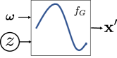
(a) Original GAN

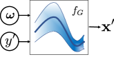
(b) BC-GAN

Figure 1: Difference between Original GAN and the Bayesian GAN proposed in this paper. In our approach, ${\boldsymbol{\omega}}$ as the parameter of the generator in original GAN is a random variable itself. Moreover, $y^{\prime}\in\mathcal{Y}$ is a deterministic label variable feed into the generator. Each sample of the data is generated from a sample of the generator function.

Similarly, we define the distribution of a set of real samples from the the discriminator as

$$p(S) = \int p({\boldsymbol{\theta}})\int p(f_{D}|{\boldsymbol{\theta}})\prod_{i=1}^{n}p(f_{D}(\mathbf{x},y_{i}))df_{D}d{\boldsymbol{\theta}}.$$

$$p(f_{D}|S) = \int p({\boldsymbol{\theta}})p(f_{D}|{\boldsymbol{\theta}})p(S|f_{D})d{\boldsymbol{\theta}}=\int p({\boldsymbol{\theta}})p(f_{D}|{\boldsymbol{\theta}})\prod_{i=1}^{n}p(f_{D}(\mathbf{x}),y_{i})d{\boldsymbol{\theta}}$$

$$p(f_{D}|S,{\boldsymbol{\theta}}) \propto p(f_{D}|{\boldsymbol{\theta}})p(S|f_{D})$$

where ${\boldsymbol{\theta}}$ is the parameter/weights of the discriminator network. These resemble Gaussian processes (GPs) for classification problems. In fact, it was shown that using the dropout in a discriminator type network resembles the posterior estimation in the GPs [6].

The advantage of using the Bayesian approaches in inference of the parameters is that we include model uncertainty in our approach and will be better equipped to tackle the convergence problem with GANs. This is because using weights from the posterior and taking advantage of the functional distribution, the learner can navigate better in the complicated parameter space. We observe that this helps with general GAN’s problem of not reaching the saddle point due to the alternation optimization in both generator and discriminator.

To estimate the expectations and perform inference we turn to commonly used Monte Carlo methods. In the following we will discuss and experiment with two of these methods. One is Markov Chain Monte Carlo and the other is Gradient Langevin dynamics. Due to uncertainty in the model and the randomness of the generator function, we observed that multiple rounds of generator update performs better in practice. In other words, we sample generator more often than updating the discriminator.

With the definitions of the distributions of generator and discriminator, we now show how to learn them below.

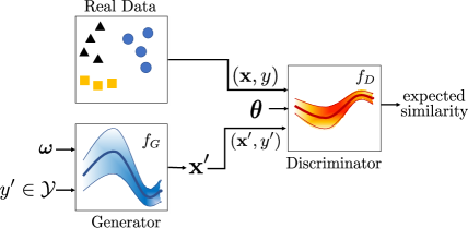
Figure 2: An illustration of the role of the generator and discriminator in our approach. Rather than

2.1 MAP Estimate and Sampling

A simple approach for using the distribution of the transformation function and the uncertainty of the discriminator is to sample from the weight distribution and then perform the GAN updates. For this, we sample the functional values of the generator and discriminator and minimize our network’s loss accordingly. This approach is on par with performing Thompson sampling used in sequential decision making where an agent picks an action iteratively to minimize an expected loss within a Bayesian framework. Here, generator and discriminator play Thompson sampling against each other where at each iteration based on the current observations (samples from the fake and real data) the distribution of discriminator (reward function) is updated .

$$\min_{{\boldsymbol{\theta}}} \mathbb{E}_{f_{D}\sim p(f_{D}|S,{\boldsymbol{\theta}})}\mathbb{E}_{(\mathbf{x},y)\sim p_{\text{data}}}[\ell_{D}(f_{D}(\mathbf{x}),y)]$$

$$\qquad\qquad\qquad-\mathbb{E}_{f_{D}\sim p(f_{D}|S,{\boldsymbol{\theta}})}\mathbb{E}_{(\mathbf{x}^{\prime},y^{\prime})\sim p_{\text{fake}}}[\ell_{G}(f_{D}(\mathbf{x}^{\prime}),y^{\prime})]\qquad\text{Discriminator Inference}$$

$$\min_{{\boldsymbol{\omega}}} \mathbb{E}_{f_{D}\sim p(f_{D}|S,{\boldsymbol{\theta}})}\Bigg{[}\mathbb{E}_{(\mathbf{x}^{\prime},y^{\prime})\sim p_{\text{fake}}}[\ell_{G}(f_{D}(\mathbf{x}^{\prime}),y^{\prime})]]$$

$$\qquad\qquad+\lambda\mathbb{E}_{(x,y)\sim p_{\text{data}}}\mathbb{E}_{(\mathbf{x}^{\prime},y^{\prime})\sim p(S^{\prime}|{\boldsymbol{\omega}})}[\Delta_{f_{D}}((\mathbf{x},y),(\mathbf{x}^{\prime},y^{\prime}))]\Bigg{]}\qquad\text{Generator Inference}$$

Here $p_{\text{data}}$ is the true underlying distribution of the data, and $p_{\text{fake}}$ is the fake distribution of the data represented by the generator. $\ell_{D}$ is the loss function of the discriminator network, and $\ell_{G}$ is the loss of the generator network. $\Delta_{f_{D}}(\mathbf{x},y),(\mathbf{x}^{\prime},y^{\prime}))$ describes the discrepancy of $(\mathbf{x},y)$ and $(\mathbf{x}^{\prime},y^{\prime})$. The overall framework of our method is shown in Figure 2.

Since Monte Carlo is an unbiased estimator of the expectations, we perform MAP on the parameters of the function and then sample the functions themselves as follows and we call this approach MAP-MC,

$$\min_{{\boldsymbol{\theta}}} L_{D}({\boldsymbol{\theta}})$$

$$\text{where }L_{D}({\boldsymbol{\theta}})=\frac{1}{n\times m}\sum_{i}\sum_{j}\ell_{D}(f_{D}^{(i)}(\mathbf{x}_{j}),y_{j})-\frac{1}{n^{\prime}\times m^{\prime}}\sum_{j}\ell_{G}(f_{D}(\mathbf{x}_{j}^{\prime}),y_{j}^{\prime})$$

$$\qquad\qquad f_{D}^{(i)}\sim p(f_{D}^{(i)}|S,{\boldsymbol{\theta}})$$

$$\min_{{\boldsymbol{\omega}}} L_{G}({\boldsymbol{\omega}})$$

$$\text{where }L_{G}({\boldsymbol{\omega}})=\frac{1}{n^{\prime}\times m^{\prime}}\sum_{j}\ell_{G}(f_{D}(\mathbf{x}_{j}^{\prime}),y_{j}^{\prime})+\frac{\lambda}{m^{\prime}}\Delta_{f_{D}^{(i)}}(S,S^{\prime})$$

$$\qquad\qquad f_{D}^{(i)}\sim p(f_{D}^{(i)}|S,{\boldsymbol{\theta}}),S^{\prime}\sim p(S^{\prime}|f_{G}^{(i)}),f_{G}^{(i)}\sim p(f_{G}^{(i)}|{\boldsymbol{\omega}})$$

2.2 Full Bayesian using Stochastic Gradient Langevin Dynamics

Another way to perform inference in our GAN model, is to employ stochastic gradient Langevin dynamics. Inspired by Robbins-Monro algorithms, this MCMC approach is proposed to perform more efficient inference in large datasets. In principle, Langevian dynamics takes the updates of the parameters in the direction of the maximum a posteriori with injecting noise so that the trajectory covers the full posterior. Thus, updating the discriminator and generator network by adding noise to the gradient of the model updates. This is particularly used when the losses $\ell_{D},\ell_{G}$ give rise to distributions e.g. in case of softmax loss.

Langevin dynamics allows us to perform the full Bayesian inference on the parameters with minor modifications to the pervious approach. To use Langevin dynamics, we update the parameters with added Gaussian noise to the gradients, i.e.

$${\boldsymbol{\theta}} = {\boldsymbol{\theta}}-\frac{\eta_{t}}{2}\times\bigg{(}\sum_{j}\nabla_{{\boldsymbol{\theta}}}L_{D}^{(j)}({\boldsymbol{\theta}})\bigg{)}+r_{t}$$

$${\boldsymbol{\omega}} = {\boldsymbol{\omega}}-\frac{\eta_{t}}{2}\times\bigg{(}\sum_{j}\nabla_{{\boldsymbol{\omega}}}L_{G}^{(j)}({\boldsymbol{\omega}})\bigg{)}+s_{t}$$ (2)

$$r_{t}\sim\mathcal{N}(0,\eta_{t}),s_{t}\sim\mathcal{N}(0,\eta_{t})$$

This added noise will ensure the parameters are not only traversing towards the mode of the distributions but also sampling them according to their density. In practice, to improve convergence of our GAN model, we use a smaller variance in noise distribution.

1:

2:$\eta:\text{learning rate}$

3:$\lambda:\text{MMD regularizer}$

4:$\pi_{D},\pi_{G}:\text{dropout probability for discriminator and generator respectively}$

5:$\sigma_{D},\sigma_{G}:\text{standard deviation of weight prior for discriminator and generator respectively}$

6:

7:Initialize ${\boldsymbol{\theta}},{\boldsymbol{\omega}}$ randomly

8:while not converged do

9:     $S=$Sample a batch $\{(\mathbf{x}_{i},y_{i})\}_{i=1}^{n}$ from the real data distribution

10:     for $j=1\to m$ do

11:         Sample $\boldsymbol{\alpha}\sim\text{Bernoulli}{(\pi_{D})}$

12:         Sample $\boldsymbol{\beta}\sim\mathcal{N}(0,\sigma_{D}^{2}\mathbf{I})$ $\triangleright$ According to dimenstions of ${\boldsymbol{\omega}}$

13:         $\tilde{{\boldsymbol{\theta}}}={\boldsymbol{\theta}}\odot\boldsymbol{\alpha}+\boldsymbol{\beta}$ $\triangleright$ Change the weights for layers of the discriminator network

14:         Compute $\nabla_{\boldsymbol{\theta}}L_{D}^{(j)}(\tilde{{\boldsymbol{\theta}}})$

15:     end for

16:     ${\boldsymbol{\theta}}={\boldsymbol{\theta}}-\eta_{t}\times\bigg{(}\sum_{j}\nabla_{\boldsymbol{\theta}}L_{D}^{(j)}(\tilde{{\boldsymbol{\theta}}})\bigg{)}$ $\triangleright$ Alternatively use Equation 2

17:     Normalize ${\boldsymbol{\theta}}$ so that $\|{\boldsymbol{\theta}}\|\leq 1$

18:     for $j=1\to m^{\prime}$ do

19:         $S^{\prime}=$SampleFake(${\boldsymbol{\omega}}$)

20:         Compute $\nabla_{\boldsymbol{\omega}}L_{G}^{(j)}(\tilde{{\boldsymbol{\omega}}})$

21:     end for

22:     ${\boldsymbol{\omega}}={\boldsymbol{\omega}}-\eta_{t}\times\bigg{(}\sum_{j}\nabla_{\boldsymbol{\omega}}L_{G}^{(j)}(\tilde{{\boldsymbol{\omega}}})\bigg{)}$ $\triangleright$ Alternatively use Equation 2

23:end while

24:return ${\boldsymbol{\theta}},{\boldsymbol{\omega}}$

25:

26:procedure SampleFake(${\boldsymbol{\omega}}$)

27:     Sample $\boldsymbol{\alpha}\sim\text{Bernoulli}{(\pi_{G})}$

28:     Sample $\boldsymbol{\beta}\sim\mathcal{N}(0,\sigma_{G}^{2}\mathbf{I})$ $\triangleright$ According to dimenstions of ${\boldsymbol{\theta}}$

29:     $\tilde{{\boldsymbol{\omega}}}={\boldsymbol{\omega}}\odot\boldsymbol{\alpha}+\boldsymbol{\beta}$ $\triangleright$ Change the weights for layers of the generator network

30:     $S^{\prime}$ = Sample a batch $\{(\mathbf{x}^{\prime}_{i},y^{\prime}_{i})\}_{i=1}^{n^{\prime}}$ from the generator network using $\tilde{{\boldsymbol{\omega}}}$

31:     return $S^{\prime}$

32:end procedure

Algorithm 1 Our Bayesian GAN algorithm.

3 Sampling Functions

At each step of our algorithm we need to compute expectations with respect to the generator and discriminators. We do this by taking samples of each function according to their distributions. This is done using simple tricks like dropout that allow us to sample from a neural network. It is shown that dropout [24] has a Bayesian interpretation where the posterior is approximated using variational inference [6]. The connection between Gaussian Processes [13, 19] and dropout for classification is made by placing a variational distribution over variables in the model and minimizing the KL-divergence between this variational distribution and the true distribution of the variables. Dropout acts as a regularizer too and improves the generalization performance of neural nets as reported in [24]. As such, we use dropout as a means of sampling various functions for the generator and discriminator.

For the discriminator, we use variants of dropout for estimating the uncertainty of the discriminator in its predictions using the variance of the predictive distribution:

$$p(y^{*}|\mathbf{x}^{*},{\boldsymbol{\theta}}) = \int p(f_{D}(\mathbf{x}^{*}),y^{*})p(f_{D}|{\boldsymbol{\theta}})df_{D}$$

$$\mathbb{E}[y^{*\top}y^{*}|\mathbf{x}^{*}] \approx \tau^{-1}\mathbf{I}+\frac{1}{m}\sum p(f_{D}(\mathbf{x}^{*}){}^{\top}f_{D}(\mathbf{x}^{*}))$$

$$\mathbb{V}[y^{*}|\mathbf{x}^{*}] \approx \mathbb{E}[y^{*\top}y^{*}|\mathbf{x}^{*}]-\mathbb{E}[y^{*}|\mathbf{x}^{*}]^{2}\qquad\qquad f_{D}=a(.,\tilde{{{\boldsymbol{\theta}}}}),\tilde{{\boldsymbol{\theta}}}={\boldsymbol{\theta}}\odot\boldsymbol{\alpha}+\boldsymbol{\beta}$$

where $a$ denotes the activation function (we slightly misused the notation for indication of the predictive mean and variance), $\tau>0$ is the variance of the prior of the weights and $\mathbf{I}$ is the identity matrix. Here, $\mathbf{x}^{*},y^{*}$ denote test instance and its corresponding predicted label either from the real or fake dataset. We use the same trick of using variants of dropout to obtain samples of the generator function too.

While GPs define distributions over functions in a non-parametric Bayesian manner by analytically integrating out the parameters, we sample the parameters and use the Monte Carlo method to estimate their expectation.

4 Choice of discrepancy measure

When the generator network generates high quality fake samples, the discrepancy between the fake samples and real samples is expected to be small. A suitable discrepancy measure should capture statistical properties of the real and fake data. We choose the maximum mean discrepancy (MMD) measure which asserts when the dimensions of the data is large and the moment matching in the input space is not possible, difference between the empirical means of two distributions using a nonlinear feature map is a measure of closeness for two-sample problems. The feature map that used in this measure has to be bounded and compact. This property is ensured by constraining the weights, i.e. $\|{\boldsymbol{\theta}}\|^{2}\leq 1$. Our $\Delta$ function is defined as,

$$\Delta_{f_{D}^{(i)}}(S,S^{\prime}) = \bigg{\|}\frac{1}{n}\sum_{l}f_{D}^{(i)}(\mathbf{x}_{l})-\frac{1}{n^{\prime}}\sum_{l^{\prime}}f_{D}^{(i)}(\mathbf{x}_{l^{\prime}}^{\prime})\bigg{\|}^{2},\qquad\qquad\|\boldsymbol{\theta}\|\leq 1$$

It is interesting to note that in the neural network implementation of this measure, we only need to ensure the parameters are normalized. The value of weight normalization in neural nets have already been shown in [21]. Here we show it can further be used in a different manner in our GAN model for density comparison.

5 Experiments

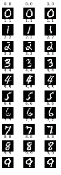
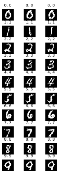
Figure 3: Samples of the conditional network in MNIST dataset using MAP-MC in Figure 3 Langevin dynamics in Figure 3.

Evaluation of generative models in general and GANs in particular is typically difficult. Since our approach has a classification loss as well, we target semi-supervised learning problems. In particular we can use small number of training instances with $\log$ loss and a softmax layer for the output of the discriminator for training our model. We also observed it is important to add an output for fake images in the loss (i.e. have $K+1$ output for the discriminator network). We use a one-hot vector of labels for the input to the generator. This deterministic input may cause collapse for the whole generator network especially if the randomizations are not enough. We add layers of dropout and Gaussian noise to every layer from the input. For all the experiments we set the batch sizes for stochastic gradient descent to $100$. We randomly select a subset of labeled examples and use the rest as unlabelled data for training. We perform these experiments $5$ times and report the mean and standard error. We use a constant learning rate for MAP-MC approach and reduce the learning rate with inversely proportionate rate with the training epoch for the Langevin dynamics. For the Monte Carlo samplings we use only $2$ samples for efficiency.

We evaluate our approach on two datasets: MNIST and CIFAR-10. In our experiments, MAP-MC performs better than Langevin dynamics in terms of accuracy that we conjecture is due to the nature of the inference method. Intuitively in Langevin dynamics, the gradients are noisy and thus the movement of the parameters in such a complex space with minimax objective is difficult.

Method/Labels	100	1000	All
Pseudo-label [12]	$10.49$	$3.64$	$0.81$
DGN [9]	$3.33\pm 0.14$	$2.40\pm 0.02$	$0.96$
Adversarial [7]			$0.78$
Virtual Adversarial [15]	$2.66$	$1.50$	$0.64\pm 0.03$
PEA [2]	$5.21$	$2.64$	$2.30$
$\Gamma\text{-Model}$ [18]	$4.34\pm 2.31$	$1.71\pm 0.07$	$0.79\pm 0.05$
BC-GAN (MAP-MC)	$1.01\pm 0.05$	$0.86\pm 0.04$	$0.7\pm 0.03$
BC-GAN (Langevin)	$2.5\pm 0.5$	$1.6\pm 0.9$	$0.8\pm 0.09$

Table 1: Semi-supervised learning using our approach compared to others on MNIST dataset. As shown approach is comparable or better than its counterparts.

MNIST Dataset: MNIST dataset contains $60,000$ training and $10,000$ test images of size $28\times 28$ of handwritten digits as greyscale images. Since the image pixels are binary, we use a generator network with sigmoid activation for the output of each pixel. For generator, we sample the one-hot label vector $y^{\prime}$ for the input uniformly for all classes (for 10 classes we have equal number of samples as the input for generator net). We use a three layer generator network with $500$ softplus activation units. In between these fully connected layers, we use Gaussian and Bernoulli dropout with variance $0.9$ and ratio $0.1$ respectively. We also used batch normalization after each layer as was shown to be effective [22].

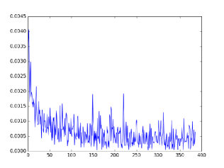
Figure 4: Predictive variance of the discriminator on 10 randomly selected samples during training in MNIST dataset using MAP-MC. In the x-axis we show the epoch and in y-axis the variance. As seen, the variance is reduced with training.

The discriminator is a fully connected network with Gaussian and Bernoulli dropout layers in between with variance $0.9$ and ratio $0.05$ respectively. We use weight normalization at the last layer (using it in all the layers seemed to improve convergence speed). As shown in Figure 3, we can generate samples of real looking images from the MNIST dataset for each label. The small numbers above generated images are the generated label and the discriminator’s prediction respectively. As observed, at the final stages of training discriminator is so powerful that can basically predict almost all generated labels correctly. Generator is also trained to match the generated class with the corresponding image. It should be noted that the samples here exploit the uncertainty of the generator network function which is desirable. Test errors for semi-supervised learning using our approach compared to the state of the art is presented in Table 1. Furthermore, predictive variance of the discriminator as a measure of its uncertainty when using only 10 labelled instances for each class is shown in Figure 4. As expected with training, the variance is reduced and the discriminator becomes more confident about its predictions.

CIFAR-10 Dataset: The CIFAR-10 dataset [11] is composed of 10 classes of natural $32\times 32$ RGB images with $50,000$ images for training and $10,000$ images for testing. Complexity of the images due to higher dimensions, color and variability make this task harder. We use a fully connected layer after the input and three layers of deconvolution that are batch normalized to generate samples. Again, we use Bernoulli and Gaussian dropout between layers with $0.9$ and ratio $0.2$ to induce uncertainty.

For the discriminator network we use a 9 layers convolutional net with two fully connected layers in the output. Furthermore, we use weight normalization at each layer. We report the performance of our approach on this dataset for semi-supervised learning in Table 2. There are samples from the generator shown in Figure 5. As observed in case of MAP-MC, we have diverse images with similarity across columns where images have same label. Langevin approach on the other hand, suffers from the mode collapse in one of the classes where some of the images seem similar (third column from left). It suggests we should have stopped earlier for the Langevin or used higher variance or ratio in dropout.

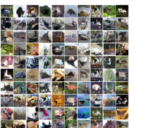
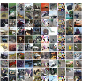
Figure 5: Samples of generated images from the CIFAR-10 dataset.

Method/Labels	1000	4000	All
Conv-Large [18, 23]		$23.3\pm 30.61$	$9.27$
$\Gamma\text{-Model}$ [18]		$20.09\pm 0.46$	$9.27$
CatGAN [22]		$19.58\pm 0.46$
Bayesian-GAN using MAP-MC	$20.9\pm 1.05$	$18.89\pm 0.65$	$7.9\pm 0.3$
Bayesian-GAN using Langevin dynamics	$25.8\pm 1.45$	$20.1\pm 1.45$	$9.3\pm 0.8$

Table 2: Test error on CIFAR10 with various number of labeled training examples.

6 Related work

Since inception of GANs [7] for unsupervised learning, various attempts have been made in either better explaining these models, extending them beyond unsupervised learning or generating more realistic samples. Wasserstein GAN [1] and Loss-Sensitive GAN [17] are recently developed theoretically grounded approaches that provide an information-theoretic view of these models. The objective in these methods are constructed to be more generic than binary classification done in the discriminator. In fact, discriminator acts as a measure of closeness for the generated samples and the real ones similar approach that is taken in this paper.

Further, GANs have been successfully used for latent variable modeling and semi-supervised learning with the intuition that the generator assists the discriminator when the number of labelled instances are small. For instance, InfoGAN [4] proposed to learn a latent variable that represents cluster of data while learning to generate images by utilizing variational inference. While it was not directly used for semi-supervised learning, its extension categorical GAN (CatGAN) [22] that utilized mutual information as part of its loss has developed with very good performance. Furthermore, [20] have developed heuristics for better training and achieving state of the art results in semi-supervised learning using GANs.

On the other hand, unlike our approach conditional GAN [14] generate labelled images by adding the label vector to the input noise. Furthermore, MMD measure [8] have been used in GANs with success [25]. However previously, kernel function had to be explicitly defined and in our approach we learn it as part of the discriminator.

Use of Bayesian methods in GANs have generally been limited to combining variational autoencoders [10] with GANs [3, 5]. We on the other hand take a Bayesian view on both discriminator and generator using the dropout approximation for variational inference. This allows us to develop a simpler and more intuitive model.

7 Conclusion

Unlike traditional GANs, we proposed a conditional Bayesian model, called BC-GAN, that exploits the uncertainty in the generator as a source of randomness for generating real samples. Similarly, we evaluate the uncertainty of the discriminator that can be used as a measure of its performance. This allows us to better analyze the behavior of a good generator/discriminator from a functional perspective for future and shed light on the GANs. We also evaluated our approach in a semi-supervised learning problem and showed its effectiveness in achieving state of the art results.

In future we plan to explore other inference methods such as Hamiltonian Monte Carlo that may yield better performance. In addition, we hope to perform more analysis on our method to better explain its internal behavior in a minimax model.

References

- [1] M. Arjovsky, S. Chintala, and L. Bottou. Wasserstein GAN. ArXiv e-prints, January 2017.
- [2] Philip Bachman, Ouais Alsharif, and Doina Precup. Learning with pseudo-ensembles. In Advances in Neural Information Processing Systems 27, pages 3365–3373. 2014.
- [3] A. Boesen Lindbo Larsen, S. Kaae Sønderby, H. Larochelle, and O. Winther. Autoencoding beyond pixels using a learned similarity metric. ArXiv e-prints, 2015.
- [4] Xi Chen, Xi Chen, Yan Duan, Rein Houthooft, John Schulman, Ilya Sutskever, and Pieter Abbeel. Infogan: Interpretable representation learning by information maximizing generative adversarial nets. In Advances in Neural Information Processing Systems 29, pages 2172–2180. 2016.
- [5] Vincent Dumoulin, Mohamed Ishmael Diwan Belghazi, Ben Poole, Alex Lamb, Martin Arjovsky, Olivier Mastropietro, and Aaron Courville. Adversarially learned inference. 2017.
- [6] Yarin Gal and Zoubin Ghahramani. Dropout as a Bayesian approximation: Representing model uncertainty in deep learning. arXiv:1506.02142, 2015.
- [7] Ian Goodfellow, Jean Pouget-Abadie, Mehdi Mirza, Bing Xu, David Warde-Farley, Sherjil Ozair, Aaron Courville, and Yoshua Bengio. Generative adversarial nets. In Advances in Neural Information Processing Systems 27, pages 2672–2680. Curran Associates, Inc., 2014.
- [8] Arthur Gretton, Karsten M Borgwardt, Malte J Rasch, Bernhard Schölkopf, and Alexander Smola. A kernel two-sample test. Journal of Machine Learning Research, 13(Mar):723–773, 2012.
- [9] Diederik P. Kingma, Shakir Mohamed, Danilo J. Rezende, and Max Welling. Semi-supervised learning with deep generative models. In Advances in Neural Information Processing Systems 27, pages 3581–3589. 2014.
- [10] Durk P. Kingma and Max Welling. Auto-encoding variational bayes. In The International Conference on Learning Representations (ICLR), 2014.
- [11] Alex Krizhevsky and Geoffrey Hinton. Learning multiple layers of features from tiny images. 2009.
- [12] Dong-Hyun Lee. Pseudo-label: The simple and efficient semi-supervised learning method for deep neural networks. In Workshop on Challenges in Representation Learning, ICML, volume 3, page 2, 2013.
- [13] David JC MacKay. Information theory, inference and learning algorithms. Cambridge university press, 2003.
- [14] M. Mirza and S. Osindero. Conditional Generative Adversarial Nets. ArXiv e-prints, November 2014.
- [15] Takeru Miyato, Shin-ichi Maeda, Masanori Koyama, Ken Nakae, and Shin Ishii. Distributional smoothing with virtual adversarial training. In International Conference on Learning Representation, 2016.
- [16] Sebastian Nowozin, Botond Cseke, and Ryota Tomioka. f-gan: Training generative neural samplers using variational divergence minimization. In Advances in Neural Information Processing Systems 29, pages 271–279. Curran Associates, Inc., 2016.
- [17] Guo-Jun Qi. Loss-sensitive generative adversarial networks on lipschitz densities. CoRR, abs/1701.06264, 2017.
- [18] Antti Rasmus, Harri Valpola, Mikko Honkala, Mathias Berglund, and Tapani Raiko. Semi-supervised learning with ladder networks. In Proceedings of the 28th International Conference on Neural Information Processing Systems, NIPS’15, pages 3546–3554, Cambridge, MA, USA, 2015. MIT Press.
- [19] Carl Edward Rasmussen and Christopher K. I. Williams. Gaussian processes for machine learning. 2006.
- [20] Tim Salimans, Ian Goodfellow, Wojciech Zaremba, Vicki Cheung, Alec Radford, Xi Chen, and Xi Chen. Improved techniques for training gans. In Advances in Neural Information Processing Systems 29, pages 2234–2242. Curran Associates, Inc., 2016.
- [21] Tim Salimans and Diederik P Kingma. Weight normalization: A simple reparameterization to accelerate training of deep neural networks. In Advances in Neural Information Processing Systems 29, pages 901–909. Curran Associates, Inc., 2016.
- [22] J. T. Springenberg. Unsupervised and semi-supervised learning with categorical generative adversarial networks. ArXiv e-prints, 2015.
- [23] Jost Tobias Springenberg, Alexey Dosovitskiy, Thomas Brox, and Martin Riedmiller. Striving for simplicity: The all convolutional net. arXiv preprint arXiv:1412.6806, 2014.
- [24] Nitish Srivastava, Geoffrey Hinton, Alex Krizhevsky, Ilya Sutskever, and Ruslan Salakhutdinov. Dropout: A simple way to prevent neural networks from overfitting. Journal of Machine Learning Research, 15:1929–1958, 2014.
- [25] D. J. Sutherland, H.-Y. Tung, H. Strathmann, S. De, A. Ramdas, A. Smola, and A. Gretton. Generative models and model criticism via optimized maximum mean discrepancy. ArXiv e-prints, 2016.