Unbound motion on a Schwarzschild background:
Practical approaches to frequency domain computations

Abstract

Gravitational perturbations due to a point particle moving on a static black hole background are naturally described in Regge-Wheeler gauge. The first-order field equations reduce to a single master wave equation for each radiative mode. The master function satisfying this wave equation is a linear combination of the metric perturbation amplitudes with a source term arising from the stress-energy tensor of the point particle. The original master functions were found by Regge and Wheeler (odd parity) and Zerilli (even parity). Subsequent work by Moncrief and then Cunningham, Price and Moncrief introduced new master variables which allow time domain reconstruction of the metric perturbation amplitudes. Here I explore the relationship between these different functions and develop a general procedure for deriving new higher-order master functions from ones already known. The benefit of higher-order functions is that their source terms always converge faster at large distance than their lower-order counterparts. This makes for a dramatic improvement in both the speed and accuracy of frequency domain codes when analyzing unbound motion.

I Introduction

The recent first detections Abbott et al. (2017a, 2016, b) of gravitational waves were made possible, in part, by accurate modeling of strongly gravitating binary sources. Through a mixture of numerical relativity, post-Newtonian theory, and black hole perturbation theory methods, the inspiral-merger-ringdown waveform is being modeled with increasing accuracy e.g. Buonanno and Damour (1999); Boh  et al. (2017); Khan et al. (2016). This work on bound motion has been incredibly important, but in the decades while these techniques have been developed, the modeling of unbound binary sources has been largely neglected.

In this work and its companion paper, Ref. Hopper and Cardoso (2017) with Cardoso, we return focus to unbound motion. In Ref. Hopper and Cardoso (2017) (and also earlier in Ref. Cardoso et al. (2016)) we provide numerical results from scattering systems, which we compare to various analytical predictions. Here, I describe the numerical method used to generate those results.

In particular, I consider point particle motion in Schwarzschild spacetime, be it a plunge or a scattering event. Finding the metric perturbation (MP) sourced by such a particle requires solving the first-order field equations. As usual, this task requires specifying a first-order gauge condition and subsequently making several choices concerning numerical techniques. Perhaps the most natural approach would be to decompose the system in spherical harmonic modes and then work in Lorenz gauge with a 1+1 time domain (TD) solver. Such an approach has been employed by Barack and Sago Barack and Sago (2010) for eccentric motion. TD codes have the advantage of being ‘source agnostic’, in that the method need not change depending on the type of motion (bound, unbound, circular). On the other hand, TD codes have the problem of junk radiation due to unphysical initial data Field et al. (2010). And, while for bound motion junk radiation will die off as the system ‘relaxes’ into the desired solution, a particle on an unbound trajectory will chase the wavefront of the junk radiation, forcing a TD simulation to begin far from the black hole, especially for high energy events. Additionally, for eccentric motion, TD codes have not been able to compete with the speed and accuracy of frequency domain (FD) approaches Akcay et al. (2013); Osburn et al. (2014); van de Meent and Shah (2015) (even for eccentricities approaching 0.8).

This advantage of FD techniques stems largely from the ease of solving a set ordinary differential equations (ODEs) rather than evolving a partial differential equation. Further, while generic source motion would have to be decomposed in the FD with a Fourier transform, bound geodesics brings the benefit of exactly periodic radial motion. Thus, the spectral decomposition of the source and its field are represented by Fourier series with exactly known frequencies. From this follows the exponential convergence of source integration Hopper et al. (2015), further improving the speed and accuracy of FD codes.

The success of FD methods for bound motion leads one to ask whether the techniques can be usefully generalized to unbound motion. The first challenge faced is the loss of the discrete spectrum provided by a Fourier series. This in itself is not an immediate reason to despair; certainly, spectral techniques are used across all areas of science to analyze non-periodic systems, usually in the form of discrete Fourier transforms. One must simply choose the largest and smallest frequencies to consider in the problem. Fundamentally, this is no different than choosing the smallest time step in a TD evolution and the total length of evolution.

The second challenge comes from considering a source which has traveled all the way from spatial infinity. Experience and physical intuition tell us that the ‘interesting part’ of the particle’s motion happens when it is (in some sense) near the black hole. Even a particle with a large Lorentz factor should simply behave as if it were in Minkowski spacetime when it is far away. Mathematically, this intuition is born out by examining the large-$r$ behavior of sources. In order to transform the TD sources to their FD amplitudes, one must (formally) integrate over all time. For such an integral to converge, the source must fall off at least a $1/r$, and indeed, examining the Lorenz gauge sources, one finds that this is always true.

And yet, of course Lorenz is not the only gauge choice available. It is often preferable to work in Regge-Wheeler (RW) gauge on Schwarzschild spacetime. Then, by employing the Regge-Wheele-Zerilli (RWZ) formalism the full field equations can be reduced to a single ‘master’ wave equation for each $\ell,m$ mode. While there appears to be little downside (at least when computing fluxes) to this approach when considering bound motion, the source terms to the master equation are not as well behaved as the Lorenz sources. The main result of this paper is to show how the RWZ sources can be modified so as to improve their large-$r$ behavior, thus improving the speed and accuracy of codes written to analyze unbound motion around a static black hole.

The numerical study of unbound point particle motion on Schwarzschild spacetime has a long history extending back to pioneering work by Davis et al. Davis et al. (1971). They used the Zerilli equation Zerilli (1970) to compute the radiated energy due to a particle falling head-on into a Schwarzschild black hole from rest at infinity. Of course, both before and since Ref. Davis et al. (1971), a variety of analytic techniques, e.g. Peters (1970); Turner (1977); Kovacs and Thorne (1978); Blanchet and Schaefer (1989), have been applied to the problem. We compare to many of those predictions in Ref. Hopper and Cardoso (2017), but they will not be considered here.

A great breakthrough in black hole perturbation theory was made by Teukolsky who derived his eponymous equation Teukolsky (1973) using the Newman-Penrose formalism. The Teukolsky equation describes scalar, neutrino, electromagnetic, and gravitational perturbations on a Kerr black hole background all in one master equation. Detweiler and Szedenits Detweiler and Szedenits (1979) made use of Teukolsky’s equation (along with a shrewd intuition for which divergent integrals to ignore) to analyze plunges with nonzero angular momentum on a Schwarzschild background.

While the Teukolsky formalism is indeed powerful, the consolidation of so many different phenomena into one equation has its costs. Two of these costs, a radial equation with a long-ranged potential and poorly behaving source terms were rectified by the transformations introduced by Sasaki and Nakamura Sasaki and Nakamura (1982). (Subsequently, the poor source term behavior was explained by Poisson Poisson (1997) and Campanelli and Lousto Campanelli and Lousto (1997).) The Sasaki-Nakamura equation has been used extensively to study unbound motion. In particular, work by Oohara Oohara (1983), Oohara and Nakamura Oohara and Nakamura (1983), and, more recently, Berti et al. Berti et al. (2010) considered the special case of static black holes.

While the Sasaki-Nakamura formalism is very powerful, I will largely ignore it here. It remains invaluable for studying point-particle motion on Kerr spacetime (especially for unbound sources), but is needlessly complicated in the Schwarzschild case. Obtaining source terms for the Sasaki-Nakamura equation requires solving an additional numerical integral, which we are able to sidestep entirely through the methods described here.

Before concluding this introduction, it is worth mentioning the relation of this work to gravitational self-force (GSF) research. Recent black hole perturbation theory methods and codes have been developed in no small part because of the desire to crack the GSF problem. The goal is to model the motion of a small-mass particle on a Kerr background while using effect of the particle’s own MP to drive it off the background geodesic. GSF research is important for the eventual detection of extreme mass-ratio binaries by LISA LIS , or a similar detector. The prospect of computing the GSF for an unbound trajectory and finding, e.g., the correction to the particle’s deflection angle is tantalizing. But, it is beyond the scope of this paper, and I will not attempt to compute the GSF here, settling for the more modest goal of developing a reliable method for finding waveforms and fluxes, which are interesting in their own right.

This paper is organized as follows. Sec. II explains the mathematical basis for the problem this paper sets out to solve. In Sec. III I explore the relationship between known master functions and also show how to generalize this relationship to define master functions with well-behaved source terms. Sec. IV gives an overview of the numerical algorithm I have implemented and discusses the practical benefits of the techniques developed here. In Sec. V I explore whether the methods presented in this paper would work in other systems. Then, the Appendix gives details of unbound geodesics, the RWZ formalism, and specific source terms. Throughout this paper I let $G=c=1$ and use standard Schwarzschild coordinates $x^{\mu}=(t,r,\theta,\varphi)$. A subscript $p$ indicates a field evaluated at the particle’s location, e.g. $r_{p}=r_{p}(t)$.

II Statement of the problem

II.1 Quick background of the RWZ formalism

I now consider the process of solving the first-order (in mass ratio) RW gauge field equations in the FD. As the general formalism has now been well established, I relegate its full presentation to App. A. For the purposes of this section it is enough to recall the following facts. The master equation in the TD is of the form

$$\begin{split}&\left[-\frac{\partial^{2}}{\partial t^{2}}+\frac{\partial^{2}}{\partial r_{*}^{2}}-V_{\ell}(r)\right]\Psi_{\ell m}(t,r)=S_{\ell m}(t,r),\end{split}$$ (1)

where $r_{*}=r+2M\log(r/2M-1)$ is the usual tortoise coordinate. Both the potential $V_{\ell}$ and the source term $S_{\ell m}$ are ($\ell+m$) parity dependent. The master function $\Psi_{\ell m}$ and its source $S_{\ell m}$ are decomposed into harmonics $X_{\ell m\omega}$ and $Z_{\ell m\omega}$ using a Fourier transform. They satisfy the FD version of Eq. (LABEL:eq:TDmastereqn),

$$\left[\frac{d^{2}}{dr_{*}^{2}}+\omega^{2}-V_{\ell}(r)\right]X_{\ell m\omega}(r)=Z_{\ell m\omega}(r).$$ (2)

It is typical to solve this equation by the method of variation of parameters, i.e. finding its homogeneous solutions (denoted $\hat{X}^{\pm}_{\ell m\omega}$, with the $+$ solution being outgoing as $r_{*}\to\infty$ and $-$ being downgoing as $r_{*}\to-\infty$) and then integrating them against the source, which has the specific distributional form $S_{\ell m}(t)\equiv G_{\ell m}(t)\,\delta(r-r_{p})+F_{\ell m}(t)\,\delta^{\prime}(r-r_{p}).$ From a practical standpoint, the crux of the numerical calculation amounts to solving the integral Hopper and Evans (2010),

$$C_{\ell m\omega}^{\pm}=\frac{1}{W_{\ell m\omega}}\int_{-\infty}^{\infty}\Bigg{[}\frac{1}{f_{p}}\hat{X}^{\mp}_{\ell m\omega}(r_{p})G_{\ell m}(t)\hskip 21.52771pt$$ (3)

$$\hskip 4.30554pt+\left(\frac{2M}{r_{p}^{2}f_{p}^{2}}\hat{X}^{\mp}_{\ell m\omega}(r_{p})-\frac{1}{f_{p}}\frac{d\hat{X}^{\mp}_{\ell m\omega}(r_{p})}{dr}\right)F_{\ell m}(t)\Bigg{]}e^{i\omega t}\,dt,$$

where $f\equiv 1-2M/r$ and $W_{\ell m\omega}$ is the Wronskian. The constants $C^{\pm}_{\ell m\omega}$ are the normalization coefficients, which must be found for a range of spherical harmonic indices $\ell,m$ and frequencies $\omega$.

For eccentric geodesic motion, the normalization coefficients, along with homogeneous solutions to Eq. (2), define the extended homogeneous solution (EHS) Barack et al. (2008), which is the correct TD solution to Eq. (LABEL:eq:TDmastereqn). The EHS method provides exponential convergence of Fourier harmonics everywhere, including the particle’s location, making it critical to fast and accurate FD GSF codes. However, in the present context one of the crucial assumptions of EHS fails, namely the presence of a source-free region where the Fourier synthesis is known to converge exponentially. As such, the EHS method is not directly applicable to unbound motion and it remains to be seen if the method can be suitably altered to once again provide exponential convergence and avoid the Gibbs behavior that results from using a singular source. For this work I do not pursue the local reconstruction of the MP, but focus rather on efficient methods for solving Eq. (3). These normalization coefficients are all that are needed to compute the waveform and the total radiated energy and angular momentum.

II.2 RWZ source behavior for various master functions

For concreteness, imagine a particle plunging from spatial infinity. It is clear that for the integral (3) to converge both $G_{\ell m}$ and $F_{\ell m}$ must fall off at least as $1/r_{p}$ far from the black hole (when $t\to-\infty$). At the horizon (when $t\to\infty$), $G_{\ell m}$ must fall off at least as $f_{p}^{2}$ while $F_{\ell m}$ must fall off at least as $f_{p}^{3}$. (Note that $\hat{X}_{\ell m\omega}^{\pm}\sim e^{\pm i\omega r_{*}}$ in the asymptotic regimes, so this does not help convergence.)

Consider now the Zerilli (Z) Zerilli (1970) source, used by Davis et al. Davis et al. (1971). (They used the axial symmetry of their problem, and so their source looks simpler than the generic source shown in App. B.) Expanding at the horizon we see,

$$G_{\ell m}^{Z}\sim f_{p}^{2}+\mathcal{O}\left(f_{p}^{3}\right),\quad F_{\ell m}^{Z}\sim f_{p}^{3}+\mathcal{O}\left(f_{p}^{4}\right),$$ (4)

as $r_{p}\to 2M.$ These converge fast enough; in fact, all master function source terms fall off sufficiently fast at the horizon, so I will not consider their expansions further. At large $r_{p}$

$$G_{\ell m}^{Z}\sim r_{p}^{-2}+\mathcal{O}\left(r_{p}^{-3}\right),\quad F_{\ell m}^{Z}\sim r_{p}^{-1}+\mathcal{O}\left(r_{p}^{-2}\right).$$ (5)

As expected, this source satisfies the necessary requirements for the convergence of the integral in Eq. (3). In the odd-parity sector, the original variable is due to Regge and Wheeler Regge and Wheeler (1957). Expanding its source at large $r_{p}$,

$$\begin{split}G_{\ell m}^{\rm RW}&\sim r_{p}^{-3}+\mathcal{O}\left(r_{p}^{-4}\right),\quad F_{\ell m}^{\rm RW}\sim r_{p}^{-3}+\mathcal{O}\left(r_{p}^{-4}\right).\end{split}$$ (6)

These terms, too, trend so that the normalization integral converges.

Recently, the original RW and Z master functions are less used because they do not permit TD reconstruction of the MP amplitudes. It is more common to use the Zerilli-Moncrief (ZM) Moncrief (1974) and Cunningham-Price-Moncrief (CPM) Cunningham et al. (1978) functions which do allow for MP reconstruction in the TD (see Martel and Poisson (2005); Hopper and Evans (2010)). The more recent ZM and CPM variables are (almost — see next section) the time integrals of the Z and RW variables. For bound motion the ZM and CPM variables are preferable in every way to the Z and RW variables. However, in the unbound case the ZM source term behaves poorly at large $r_{p}$,

$$\begin{split}G_{\ell m}^{\rm ZM}&\sim r_{p}^{-1}+\mathcal{O}\left(r_{p}^{-2}\right),\quad F_{\ell m}^{\rm ZM}\sim r_{p}^{0}+\mathcal{O}\left(r_{p}^{-1}\right).\end{split}$$ (7)

The $F^{\rm ZM}_{\ell m}$ term prevents the normalization integral (3) from converging. Meanwhile the CPM variable still converges at large $r_{p}$ implying that it can be used to analyze unbound sources, but is less effective than the RW variable since it falls off significantly more slowly,

$$\begin{split}G_{\ell m}^{\rm CPM}&\sim r_{p}^{-2}+\mathcal{O}\left(r_{p}^{-3}\right),\ \ F_{\ell m}^{\rm CPM}\sim r_{p}^{-1}+\mathcal{O}\left(r_{p}^{-2}\right).\end{split}$$ (8)

In the next section, by examining the ways in which the different variables are related, I develop a general method for constructing master functions with progressively higher-order large $r_{p}$ convergence.

III Time derivatives of master functions

Beginning in this section I drop $\ell m$ indices for brevity, although I do indicate FD quantities with a subscript $\omega$. I use the harmonic decomposition and MP notation introduced by Martel and Poisson Martel and Poisson (2005) with source term notation from Hopper and Evans Hopper and Evans (2010). Also, I define the symbols $\lambda\equiv(\ell+2)(\ell-1)/2$, $\Lambda\equiv\lambda+3M/r$.

III.1 Relationships between the known master functions

III.1.1 Odd parity

The CPM master function is defined through the following linear combination of odd-parity RW gauge MP amplitudes and their first derivatives,

$$\Psi_{\rm CPM}^{(0)}(t,r)\equiv\frac{r}{\lambda}\left(\partial_{r}h_{t}-\partial_{t}h_{r}-\frac{2}{r}h_{t}\right).$$ (9)

The superscript $(0)$ indicates the number of time derivatives of the CPM variable. This is a $C^{-1}$ function (that is, it has a jump in its value at the particle’s location, but is otherwise smooth), and so taking its time derivative (indicated with a dot) yields a distribution with a time-dependent Dirac delta at the particle’s location,

$$\begin{split}\dot{\Psi}_{\rm CPM}^{(0)}(t,r)&=\frac{r}{\lambda}\left(\partial_{t}\partial_{r}h_{t}-\partial_{t}^{2}h_{r}-\frac{2}{r}\partial_{t}h_{t}\right)\\ &=\frac{2f}{r}h_{r}-\frac{r_{p}f_{p}}{\lambda}p_{r}(t)\delta\left(r-r_{p}\right),\end{split}$$ (10)

where the second equality follows from the field equations (see Hopper and Evans (2010)). Since we know the magnitude of the delta function exactly, we subtract it off, defining a new master function which is also $C^{-1}$,

$$\Psi_{\rm CPM}^{(1)}(t,r)\equiv\dot{\Psi}_{\rm CPM}^{(0)}+\frac{r_{p}f_{p}}{\lambda}p_{r}(t)\delta\left(r-r_{p}\right)=\frac{2f}{r}h_{r}.$$ (11)

The superscript $(1)$ means “the first time derivative of the CPM variable with the singular part subtracted.” This is exactly twice the original RW variable. Except for exactly at the location of the particle, it is precisely the time derivative of the CPM variable. Therefore, the normalization coefficients for $\Psi^{(0)}_{\rm CPM}$ are related to those of $\Psi^{(1)}_{\rm CPM}$ by

$$C^{(0),\pm}_{{\rm CPM},\omega}=\frac{C^{(1),\pm}_{{\rm CPM},\omega}}{-i\omega}.$$ (12)

which is valid for all $\omega\neq 0$. The $\omega\to 0$ limit is subtle for unbound motion and is discussed at length in Ref. Hopper and Cardoso (2017).

III.1.2 Even parity

The ZM function is defined as

$$\Psi_{\rm ZM}^{(0)}(t,r)\equiv\frac{r}{\lambda+1}\left[K+\frac{1}{\Lambda}\left(f^{2}h_{rr}-rf\partial_{r}K\right)\right].$$ (13)

It, too, is $C^{-1}$, so taking its time derivative introduces a Dirac delta,

$$\dot{\Psi}_{\rm ZM}^{(0)}(t,r)=\frac{r}{\lambda+1}\left[\partial_{t}K+\frac{1}{\Lambda}\left(f^{2}\partial_{t}h_{rr}-rf\partial_{t}\partial_{r}K\right)\right]$$

$$=\frac{1}{\Lambda}\left(r\partial_{t}K-fh_{tr}\right)+\frac{r_{p}^{2}f_{p}}{\Lambda_{p}(\lambda+1)}q_{tr}(t)\delta\left(r-r_{p}\right),$$ (14)

where again I have used the field equations. After subtracting the singular term, define a new master function which is also $C^{-1}$,

$$\begin{split}\Psi_{\rm ZM}^{(1)}(t,r)&\equiv\dot{\Psi}_{\rm ZM}^{(0)}-\frac{r_{p}^{2}f_{p}}{\Lambda_{p}(\lambda+1)}q_{tr}(t)\delta\left(r-r_{p}\right)\\ &=\frac{1}{\Lambda}\left(r\partial_{t}K-fh_{tr}\right).\end{split}$$ (15)

This is exactly the original Zerilli variable (although he wrote it in the FD). Except at the exact location of the particle, it is precisely the time derivative of the ZM variable. As before, note that the $\Psi_{\rm ZM}^{(0)}$ and $\Psi_{\rm ZM}^{(1)}$ normalization coefficients are related via

$$C^{(0),\pm}_{{\rm ZM},\omega}=\frac{C^{(1),\pm}_{{\rm ZM},\omega}}{-i\omega}.$$ (16)

The conclusion to draw from these variables is, taking the time derivative of a master functions and then removing the offending Dirac delta will always produce a new master function of the same form.

III.2 Master functions with an arbitrary number of time derivatives

In the previous subsection, I showed that one can derive one master function from another by taking the time derivative and subtracting the exact delta function that follows from differentiating a $C^{-1}$ function. Now I generalize that process to show how one can differentiate arbitrarily many times, each time creating a new master function of the same form.

Consider a master function $\Psi^{(0)}$ which satisfies an equation of the form

$$\begin{split}&\left[-\frac{\partial^{2}}{\partial t^{2}}+\frac{\partial^{2}}{\partial r_{*}^{2}}-V(r)\right]\Psi^{(0)}(t,r)\\ &\hskip 43.05542pt=G^{(0)}(t)\delta\left(r-r_{p}\right)+F^{(0)}(t)\delta^{\prime}\left(r-r_{p}\right).\end{split}$$ (17)

It is convenient to write the master function in the weak form

$$\Psi^{(0)}(t,r)=\Psi^{(0),+}(t,r)\theta\left(r-r_{p}\right)+\Psi^{(0),-}(t,r)\theta\left(r_{p}-r\right).$$ (18)

The Heaviside coefficients satisfy the homogeneous version of Eq. (LABEL:eq:master1), while the source terms imply that the jump in $\Psi^{(0)}$ at the particle’s location is Hopper and Evans (2010)

$$\llbracket\Psi^{(0)}\rrbracket_{p}(t) =\frac{\mathcal{E}^{2}}{f_{p}^{2}U_{p}^{2}}F^{(0)}.$$ (19)

$\mathcal{E}$ is the particle’s specific energy and $U_{p}^{2}$ is the effective potential, defined in App. A. Now, we can take the time derivative of any master function that satisfies Eq. (LABEL:eq:master1) and it will satisfy an equation of the same form. However, the time derivative will introduce a second derivative of the delta function in the source on the RHS. This follows because the time derivative of $\Psi^{(0)}$ is

$$\begin{split}\dot{\Psi}^{(0)}(t,r)=&\dot{\Psi}^{(0),+}\theta\left(r-r_{p}\right)+\dot{\Psi}^{(0),-}\theta\left(r_{p}-r\right)\\ &-\dot{r}_{p}\llbracket\Psi^{(0)}\rrbracket_{p}\delta\left(r-r_{p}\right).\end{split}$$ (20)

Thus, I define

$$\Psi^{(1)}(t,r) \equiv\dot{\Psi}^{(0)}+\frac{\dot{r}_{p}\mathcal{E}^{2}}{f_{p}^{2}U_{p}^{2}}F^{(0)}\delta\left(r-r_{p}\right),$$ (21)

which is $C^{-1}$ and will satisfy an equation of the form (LABEL:eq:master1) with no $\delta^{\prime\prime}(r-r_{p})$ source term.

III.3 Higher-order source terms

It is fine to define new master functions by differentiating the old functions, but what makes a master function unique is its source term. In order to find the source term for $\Psi^{(1)}$, start by acting with the wave operator on Eq. (21),

$$\left[-\frac{\partial^{2}}{\partial t^{2}}+\frac{\partial^{2}}{\partial r_{*}^{2}}-V(r)\right]\left[\dot{\Psi}^{(0)}+\frac{\dot{r}_{p}\mathcal{E}^{2}}{f_{p}^{2}U_{p}^{2}}F^{(0)}\delta\left(r-r_{p}\right)\right]=G^{(1)}\delta(r-r_{p})+F^{(1)}\delta^{\prime}(r-r_{p}).$$ (22)

When the wave operator hits $\dot{\Psi}^{(0)}$, it is equivalent to taking the time derivative of Eq. (LABEL:eq:master1) and so

$$\begin{split}&\left[-\frac{\partial^{2}}{\partial t^{2}}+\frac{\partial^{2}}{\partial r_{*}^{2}}-V(r)\right]\left[\frac{\dot{r}_{p}\mathcal{E}^{2}}{f_{p}^{2}U_{p}^{2}}F^{(0)}\delta\left(r-r_{p}\right)\right]+\dot{G}^{(0)}\delta(r-r_{p})+\left(\dot{F}^{(0)}-G^{(0)}\dot{r}_{p}\right)\delta^{\prime}(r-r_{p})\\ &\hskip 236.80481pt-F^{(0)}\dot{r}_{p}\delta^{\prime\prime}(r-r_{p})=G^{(1)}\delta(r-r_{p})+F^{(1)}\delta^{\prime}(r-r_{p}).\end{split}$$ (23)

Acting on the remaining delta term requires care. The $r_{*}$ derivatives must be expanded as $\partial^{2}_{r_{*}}=f(r)\partial_{r}f(r)\partial_{r}$, and then any functions of $r$ must be evaluated at $r=r_{p}(t)$ by using the identities (for a smooth test function $g$)

$$\begin{split}g(x)\ \delta(x)&=g(0)\ \delta(x),\\ g(x)\ \delta^{\prime}(x)&=g(0)\ \delta^{\prime}(x)-g^{\prime}(0)\ \delta(x),\\ g(x)\ \delta^{\prime\prime}(x)&=g(0)\ \delta^{\prime\prime}(x)-2g^{\prime}(0)\ \delta^{\prime}(x)+g^{\prime\prime}(0)\ \delta(x).\end{split}$$ (24)

By design the $\delta^{\prime\prime}(r-r_{p})$ term cancels. Then, equating the remaining coefficients of $\delta(r-r_{p})$ and $\delta^{\prime}(r-r_{p})$ respectively yields

$$\begin{split}G^{(1)}=&\ \dot{G}^{(0)}-\frac{\mathcal{E}^{2}\dot{r}_{p}\ddot{F}^{(0)}}{f_{p}^{2}U_{p}^{2}}+\frac{2\dot{F}^{(0)}}{r_{p}^{7}U_{p}^{4}}\bigg{[}10\mathcal{L}^{4}M^{2}-7\mathcal{L}^{4}Mr_{p}+\left(\mathcal{L}^{4}+16\mathcal{L}^{2}M^{2}\right)r_{p}^{2}+2\mathcal{L}^{2}M\left(4\mathcal{E}^{2}-5\right)r_{p}^{3}\\ &+\left(6M^{2}+\mathcal{L}^{2}-2\mathcal{L}^{2}\mathcal{E}^{2}\right)r_{p}^{4}+M\left(4\mathcal{E}^{2}-3\right)r_{p}^{5}\bigg{]}+\frac{\dot{r}_{p}F^{(0)}}{r_{p}^{11}U_{p}^{6}}\Bigg{[}-\frac{\mathcal{E}^{2}r_{p}^{11}U_{p}^{4}V_{p}}{f_{p}^{2}}+20\mathcal{L}^{6}M^{3}-30\mathcal{L}^{6}M^{2}r_{p}\\ &+4\mathcal{L}^{4}M\left(17M^{2}+3\mathcal{L}^{2}\right)r_{p}^{2}-\mathcal{L}^{4}\left(\mathcal{L}^{2}+20\mathcal{E}^{2}M^{2}+102M^{2}\right)r_{p}^{3}+\left(60\mathcal{L}^{2}M^{3}+8\mathcal{L}^{4}\mathcal{E}^{2}M+42\mathcal{L}^{4}M\right)r_{p}^{4}\\ &-2\mathcal{L}^{2}\left(45M^{2}-12\mathcal{E}^{2}M^{2}+\mathcal{L}^{2}\mathcal{E}^{2}+2\mathcal{L}^{2}\right)r_{p}^{5}+12M\left(M^{2}-3\mathcal{L}^{2}\mathcal{E}^{2}+3\mathcal{L}^{2}\right)r_{p}^{6}\\ &+3\left(4\mathcal{E}^{2}M^{2}-6M^{2}+2\mathcal{L}^{2}\mathcal{E}^{2}-\mathcal{L}^{2}\right)r_{p}^{7}+6M\left(1-2\mathcal{E}^{2}\right)r_{p}^{8}\Bigg{]}\end{split}$$ (25)

$$\begin{split}F^{(1)}=&-\dot{r}_{p}G^{(0)}+\frac{\dot{F}^{(0)}}{U_{p}^{2}r_{p}^{3}}\Big{[}2\mathcal{L}^{2}M-\mathcal{L}^{2}r_{p}+2Mr_{p}^{2}+\left(2\mathcal{E}^{2}-1\right)r_{p}^{3}\Big{]}+\frac{F^{(0)}\dot{r}_{p}}{r_{p}^{7}U_{p}^{4}}\bigg{[}-10\mathcal{L}^{4}M^{2}+7\mathcal{L}^{4}Mr_{p}\\ &-\left(\mathcal{L}^{4}+16\mathcal{L}^{2}M^{2}\right)r_{p}^{2}+10\mathcal{L}^{2}M\left(1-2\mathcal{E}^{2}\right)r_{p}^{3}-\left(6M^{2}+\mathcal{L}^{2}-4\mathcal{L}^{2}\mathcal{E}^{2}\right)r_{p}^{4}+3M\left(1-4\mathcal{E}^{2}\right)r_{p}^{5}\bigg{]}\end{split}$$ (26)

In writing these, I have used the constraints in Eq. (37) to reduce the number (and order of) time derivatives of $r_{p}$. Note the $V_{p}$ term in Eq. (25), which is the (parity-appropriate) potential evaluated at $r=r_{p}$.

The expressions (25) and (26) are generic relations between the source terms of any two master functions of different ‘order’. It is a straightforward (if tedious) task to insert the $G$ and $F$ terms from the CPM (or ZM) variable on the RHS and obtain the $G$ and $F$ terms from the RW (or Z) variable. It remains to show that the higher-order source terms converge more quickly at large $r_{p}$ than the lower-order ones.

Expanding each of the terms on the RHS of Eq. (25) in inverse powers of $r_{p}$ confirms that $G^{(1)}$ is guaranteed to fall off at least one power of $r_{p}$ faster than $G^{(0)}$. Meanwhile, $F^{(1)}$ is guaranteed to converge at least as fast as $F^{(0)}$. It is evident that if $F^{(1)}$ does not ‘out-converge’ $F^{(0)}$, then proceeding to the next order will produce a new source $F^{(2)}$, which will converge faster. This exact phenomenon occurs in the right panel of Fig. 1 when $F^{(3)}_{\rm ZM}$ converges at the same rate as $F^{(2)}_{\rm ZM}$, but then $F^{(4)}_{\rm ZM}$ converges more rapidly.

Since the master functions $\Psi^{(1)}$ is essentially the time-derivative of $\Psi^{(0)}$, the two functions have associated normalization coefficients related by $C_{\omega}^{(0),\pm}=C_{\omega}^{(1),\pm}/(-i\omega).$ Each higher order brings one extra factor of $(-i\omega)^{-1}$. By adjusting the normalization coefficients this way, one can always get back to the CPM and ZM variables which allow TD MP reconstruction.

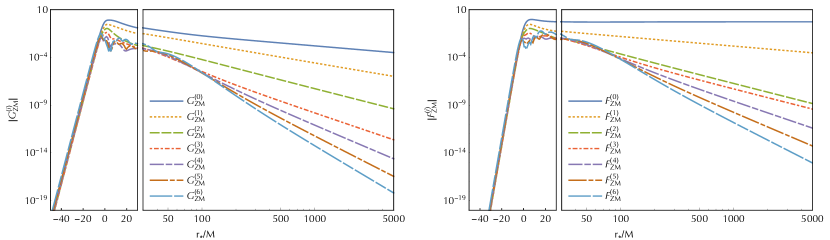
Figure 1: The $(\ell,m)=(2,2)$ mode source terms for a plunging particle with $\mathcal{E}=3$ and $\mathcal{L}_{\rm frac}=0.99$ (see App. A.1 for orbit parametrization). In each of these graphs, the left side shows a log-linear plot, emphasizing the exponential decay of the source terms at the horizon. On the right of each graph, the horizontal axis changes to logarithmic, displaying the algebraic convergence at large distance. Note that $F_{\rm ZM}^{(0)}$, the ZM source, does not converge [see Eq. (7)]. The next-order source term ($F_{\rm ZM}^{(1)}$) converges only as $r_{p}^{-1}$, while the second-order term ($F_{\rm ZM}^{(2)}$) jumps to an efficient $r_{p}^{-3}$ convergence.

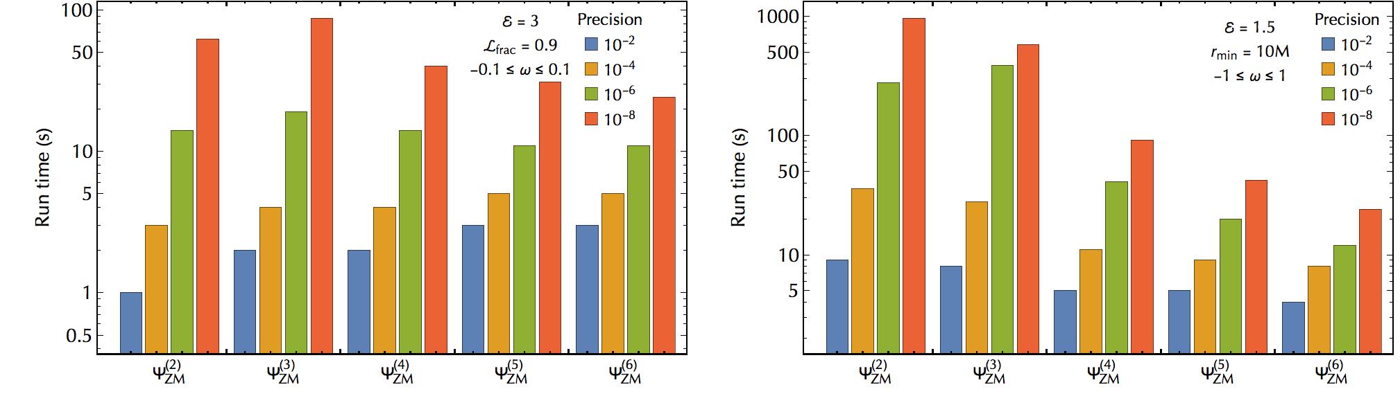
Figure 2: Run times for a variety of precision requirements and master function choices. All runs are for the $(\ell,m)=(2,2)$ mode and 20 evenly spaced harmonics in the shown $\omega$ range (excluding $\omega=0$). The plots show that the benefit of high-order master functions are realized when $\omega$ gets large. See also discussion in the text.

IV Implementation and Results

IV.1 Numerical implementation

I now briefly describe the algorithmic details of my numerical implementation. The code is written in $C$, uses a GSL integrator GSL , and works in the following series of steps.

1. Solve geodesic equations. A discussion of unbound geodesics is given in App. A.

2. Find boundary conditions to homogeneous FD master equation (2) for a given $\ell,m,\omega$ mode. The infinity-side (out-going wave) solution is found with an asymptotic expansion in $(\omega r)^{-1}$ while the horizon-side (down-going wave) solution is found from a Taylor expansion in $f$. This is equivalent to the way homogeneous solutions are found in the bound case, e.g. Hopper and Evans (2010).

3. Integrate homogeneous solutions to source boundary. Numerically integrate both homogeneous solutions to the point where the source is closest to the black hole. For scattering events this is the periapsis $r_{\rm min}$. For plunging trajectories, usually around $r_{*}=-40M$ is plenty close (note the magnitude of the source terms there in Fig. 1).

4. Concurrently integrate homogeneous solutions with normalization integral, (3). Starting close to the black hole, numerically integrate out to a large $r_{p}$. Then, double $r_{p}$, integrate again and check for convergence of Eq. (3). App. A has a brief discussion of the best independent variables to use for this integral. Note that for plunges, the horizon flux, and hence the $C^{-}_{\ell m\omega}$ integral is known to diverge, Davis et al. (1972). For the scattering case, there are two (asymmetric, due to $\dot{r}_{p}$ terms) legs of the trajectory, which both must be covered in the source integration.

5. Repeat steps $2-4$ for a range of $\ell,m,\omega$. While $m$ always ranges from $-\ell$ to $\ell$, both $\ell$ and $\omega$ have infinite range (with each $\omega$ spectrum being dense). The choice of how to truncate (and discretize) these ranges rests on overall accuracy requirements.

For fluxes, the $\ell$-sum consistently converges exponentially, so choosing where to stop that infinite sum is straightforward. For a given $\ell,m$ though, the relevant range of $\omega$ to choose is far from obvious. Weaker-field events radiate less and require a finer discretization of the $\omega$ range. Further, the energy spectrum of any given $\ell,m$ mode exhibits numerous ‘zeros’ where the spectrum vanishes for a given $\omega$, only to rise again beyond that point, making detecting spectral convergence quite challenging. Thus, a fair amount of logic must be programmed into any algorithm in order for it to dynamically determine how to truncate these infinite sums. The features of the energy spectrum discussed here can be seen in the figures of the accompanying work Ref. Hopper and Cardoso (2017).

A last challenge with the $\omega$-spectrum is the static mode $\omega=0$. Smarr Smarr (1977) pointed out that the energy spectrum goes to a constant in this limit whenever the particle’s speed is non-zero at infinity. It is simplest to consider very small modes, but skip the static mode itself. We explore the zero-frequency limit thoroughly in Hopper and Cardoso (2017).

IV.2 Practical effects of higher-order master functions

At first glance, there appears no downside to using higher-order master functions. Certainly, ever higher-order functions do provide ever-faster converging source terms. However, in attempting to implement such a scheme, practical issues quickly arise. First, after the first two orders, the new source terms quickly become large, so large in fact that the straightforward evaluation of them starts to outweigh the benefits of faster $r_{p}$-convergence. To some extent, this trouble can be sidestepped by an efficiently written code. It is best to precompute position independent terms that show up in $G$ and $F$ before performing the normalization integral. Even then, the choice of which master function to use is not obvious, as can be seen in Fig. 2.

The figure shows two separate runs, performed for a range of precision requirements with various master functions. Looking at the left panel, we see that when $\omega$ is relatively small (in magnitude), there is little effect on run times from choosing a different master function. For high precision requirements, the higher-order function does lead to faster runs, but the benefit is minor. For low precision, increasing the order of the master function actually worsens the runs times. The benefit of a higher-order master function becomes evident at larger frequencies. In the right panel of Fig. 2, the high-order master functions out-perform the lower-order functions significantly, especially when precision requirements are high. The most significant feature of this figure is what is not shown, namely Zerilli’s original variable $\Psi_{\rm ZM}^{(1)}$. As discussed, the source term for $\Psi_{\rm ZM}^{(1)}$ decays like $r_{p}^{-1}$, which is slow enough to make numerical convergence to high precision impossible.

If one is not interested in results with precision beyond (say) $10^{-4}$ and only considering moderately large-$\omega$ (which excludes ultrarelativistic events), the high-order master functions are usually unnecessary. The new even-parity master function $\Psi_{\rm ZM}^{(2)}$ and the original odd-parity RW function $\Psi_{\rm CPM}^{(1)}$ provide a convenient ‘sweet-spot’ of fast $r_{p}$-convergence with relatively compact source terms. They are each given in App. B. For high-energy runs though, the relevant range of harmonics gets high, and the benefit of higher-order master functions is substantial.

Figure 3: Example results from the code presented here. Both panels show the $(\ell,m)=(2,2)$ modes of the TD waveforms. The left panel gives a sample waveform for a scattering run, and the right considers a sample plunge. Many more results from scattering runs computed with this code can be found in Ref. Hopper and Cardoso (2017).

V Prospects for application to other formalisms and problems

The methods developed here to improve source behavior at large distances are ideally suited to the RWZ formalism. It is worth exploring to what extent the same techniques could be applied to other systems.

V.1 Lorenz gauge on Schwarzschild

The most natural extension of this technique would be to the Lorenz gauge field equations on Schwarzschild spacetime. As mentioned, there should be no trouble using the equations in their natural form since each of the source terms falls off as $1/r_{p}^{2}$ at large $r_{p}$. However, especially for large Lorentz factors it is useful to have source terms which fall off even faster. Without working out the details, I will show why we can probably increase the rate of large-$r$ source convergence.

In the TD, each of the (unconstrained) Lorenz gauge field equations is of the form

$$\begin{split}\left(-\frac{\partial^{2}}{\partial t^{2}}+\frac{\partial^{2}}{\partial r_{*}^{2}}\right)h^{(0)}_{i}(t,r)+\mathcal{M}_{ij}h^{(0)}_{j}(t,r)\\ =S^{(0)}_{i}(t)\delta\left(r-r_{p}\right),\end{split}$$ (27)

where $h^{(0)}_{i}$ represents any of the 10 MP amplitudes ($h_{tt},h_{tr},h_{rr},j_{t},j_{r}K,G,h_{t},h_{r},h_{2}$), $\mathcal{M}_{ij}$ is a matrix coupling the fields and their first derivatives, and $S_{i}^{(0)}(t)$ are the source amplitudes coming from the particle’s stress energy projection. The structure of the Lorenz gauge equations, with a wave operator on the LHS and only a delta function (no delta prime) on the RHS implies that each of the amplitudes $h^{(0)}_{i}$ is $C^{0}$. Taking one time derivative yields

$$\begin{split}&\left(-\frac{\partial^{2}}{\partial t^{2}}+\frac{\partial^{2}}{\partial r_{*}^{2}}\right)\dot{h}^{(0)}_{i}(t,r)+\mathcal{M}_{ij}\dot{h}^{(0)}_{j}(t,r)\\ &\hskip 21.52771pt=\dot{S}_{i}^{(0)}(t)\delta\left(r-r_{p}\right)-\dot{r}_{p}S_{i}^{(0)}(t)\delta^{\prime}\left(r-r_{p}\right),\end{split}$$ (28)

The delta prime on the RHS implies that the fields $\dot{h}^{(0)}_{i}$ are $C^{-1}$ with jumps equal to

$$\llbracket\dot{h}^{(0)}_{i}\rrbracket_{p}(t)=-\frac{\dot{r}_{p}\mathcal{E}^{2}}{f_{p}^{2}U_{p}^{2}}S_{i}^{(0)}.$$ (29)

Taking the second time derivative of the field equations gives

$$\begin{split}&\left(-\frac{\partial^{2}}{\partial t^{2}}+\frac{\partial^{2}}{\partial r_{*}^{2}}\right)\ddot{h}^{(0)}_{i}(t,r)+\mathcal{M}_{ij}\ddot{h}^{(0)}_{j}(t,r)\\ &\hskip 21.52771pt=\ddot{S}_{i}^{(0)}\delta\left(r-r_{p}\right)-2\dot{r}_{p}\dot{S}_{i}^{(0)}\delta^{\prime}\left(r-r_{p}\right)\\ &\hskip 34.44434pt-\ddot{r}_{p}S_{i}^{(0)}\delta^{\prime}\left(r-r_{p}\right)+\dot{r}^{2}_{p}S_{i}^{(0)}\delta^{\prime\prime}\left(r-r_{p}\right).\end{split}$$ (30)

The $\delta^{\prime\prime}(r-r_{p})$ source implies a $\delta(r-r_{p})$ term in each $\ddot{h}^{(0)}_{i}$ with a coefficient of $-\dot{r}_{p}\llbracket\dot{h}^{(0)}_{i}\rrbracket_{p}$. Subtracting this term, we can define a new set of amplitudes

$$h^{(2)}_{i}(t,r)\equiv\ddot{h}^{(0)}_{i}(t,r)-\frac{\dot{r}_{p}^{2}\mathcal{E}^{2}}{f_{p}^{2}U_{p}^{2}}S_{i}^{(0)}\delta\left(r-r_{p}\right),$$ (31)

which are all $C^{-1}$. They are exactly the second time derivative of the Lorenz gauge fields, except at the exact location of the particle. These fields satisfy equations of the form

$$\begin{split}&\left(-\frac{\partial^{2}}{\partial t^{2}}+\frac{\partial^{2}}{\partial r_{*}^{2}}\right)h^{(2)}_{i}(t,r)+\mathcal{M}_{ij}h^{(2)}_{j}(t,r)\\ &\hskip 21.52771pt=S_{i}^{(2)}(t)\delta\left(r-r_{p}\right)+R_{i}^{(2)}(t)\delta^{\prime}\left(r-r_{p}\right).\end{split}$$ (32)

The differential operator on the LHS is precisely the Lorenz gauge operator. It remains to act with Eq. (LABEL:eq:h2Eq) on the new fields (31) to derive expressions for the new source terms $S_{i}^{(2)}$ and $R_{i}^{(2)}$. The output is too lengthy and tedious to include here, but I have done so and seen that each term decays at least as $r_{p}^{-3}$, indicating that source integrations would converge more quickly by using $S_{i}^{(2)}$ and $R_{i}^{(2)}$ source terms rather than $S_{i}^{(0)}$. Note that if this method were employed, the normalization procedure laid out in Refs. Akcay et al. (2013) and Osburn et al. (2014) would have to be modified slightly in order to take into account the delta prime in the source. Lastly, it is worth remembering that the primary reason to use the Lorenz gauge equations is for local GSF calculations, but this paper has not addressed local calculations.

V.2 Unbound motion on Kerr

The situation on Kerr is less promising. Perturbations on a Kerr background are typically found by solving the Teukolsky equation. It is a wave operator in all four spacetime variables acting on either of the Weyl scalars $\psi_{4}$ or $\psi_{0}$. Schematically it is of the form

$$\mathcal{W}\big{[}\psi(t,r,\theta,\varphi)\big{]}=G(t)\delta^{3}\left(x^{i}-x^{i}_{p}\right)$$ (33)

$$\hskip 8.61108pt+F_{j}(t)\partial_{j}\delta^{3}\left(x^{i}-x^{i}_{p}\right)+E_{jk}(t)\partial_{j}\partial_{k}\delta^{3}\left(x^{i}-x^{i}_{p}\right),$$

where the indices $i,j,k$ range over $r,\theta,\varphi$. One can exploit the axial symmetry of the Kerr background and reduce the $3+1$ Teukolsky equation to a set (over azimuthal number $m$) of $2+1$ equations, at which point the schematic form is

$$\mathcal{W}_{m}\big{[}\psi_{m}(t,r,\theta)\big{]}=G^{m}(t)\delta^{2}\left(x^{a}-x^{a}_{p}\right)$$ (34)

$$\hskip 8.61108pt+F^{m}_{b}(t)\partial_{b}\delta^{2}\left(x^{a}-x^{a}_{p}\right)+E^{m}_{bc}(t)\partial_{b}\partial_{c}\delta^{2}\left(x^{a}-x^{a}_{p}\right),$$

where the indices $a,b,c$ range over $r,\theta$.

Unfortunately, the Teukolsky equation has never been decomposed into a decoupled set of $1+1$ equations in $t$ and $r$. In order to decompose it further, one must go all the way to the FD and obtain an ODE in $r$ (as well as a separate homogeneous ODE in $\theta$). The method I have presented in this paper relies on a $1+1$ wave equation and detailed knowledge of the weak structure of the field at the particle’s location. One can imagine taking a similar approach to the $2+1$ equation (34), but problems quickly arise. The issue is that the distributions on the RHS of Eq. (34) do not stem from taking derivatives of Heavisides and Dirac deltas. Rather, they are due to the local $1/r$ divergence of the particle’s own field. An attempt to write down a $2+1$ weak form of $\psi_{m}(t,r,\theta)$ akin to that in Eq. (18) succeeds only in the sense that the coefficients of the Heavisides are not finite at $(r,\theta)=(r_{p},\theta_{p})$. Indeed, this very divergence is at the heart of all GSF research over the last two decades.

It seems then that the best bet for applying the methods developed in this paper would be to decompose Eq. (34) into a coupled set of 1+1 equations. Clearly, this is not ideal, and it is worth admitting that the Sasaki-Nakamura formalism is probably a far simpler and more effective way to study unbound motion on Kerr.

Appendix A The RWZ formalism

A.1 Unbound Schwarzschild geodesics

Consider a point particle of mass $\mu$ moving on a Schwarzschild background of mass $M$. Let the worldline be parametrized by proper time $\tau$, i.e. $x_{p}^{\mu}(\tau)=\left[t_{p}(\tau),r_{p}(\tau),\pi/2,\varphi_{p}(\tau)\right]$, where I have confined the particle to $\theta_{p}=\pi/2$ without loss of generality. Generic geodesics are parametrized by the specific energy $\mathcal{E}$ and the specific angular momentum $\mathcal{L}$. The four-velocity $u^{\mu}=dx_{p}^{\mu}/d\tau$ can be written in terms of them as

$$u^{t}=\frac{\mathcal{E}}{f_{p}},\quad\quad u^{\varphi}=\frac{{\cal{L}}}{r_{p}^{2}},\quad\quad\left(u^{r}\right)^{2}=\mathcal{E}^{2}-U^{2}_{p},$$ (35)

where the effective potential is

$$U^{2}(r,\mathcal{L}^{2})\equiv f\left(1+\frac{\mathcal{L}^{2}}{r^{2}}\right).$$ (36)

The radial coordinate velocity obeys the constraints

$$\begin{split}\dot{r}_{p}^{2}(t)&=f_{p}^{2}-\frac{f_{p}^{2}}{{\cal{E}}^{2}}U^{2}_{p},\\ \ddot{r}_{p}(t)&=\frac{2Mf_{p}}{r_{p}^{2}}-\frac{f_{p}^{2}}{{\cal{E}}^{2}r_{p}^{2}}\left[3M-\frac{{\cal{L}}^{2}}{r_{p}}+\frac{5M{\cal{L}}^{2}}{r_{p}^{2}}\right].\end{split}$$ (37)

A.1.1 Plunges

Geodesics representing particles plunging from infinity must have $\mathcal{E}\geq 1$ and also clear the peak of the effective potential,

$$U^{2}_{\rm max}=\frac{1}{54}\left[\frac{\mathcal{L}^{2}}{M^{2}}+36+\sqrt{1-\frac{12M^{2}}{\mathcal{L}^{2}}}\left(\frac{\mathcal{L}^{2}}{M^{2}}-12\right)\right].$$ (38)

Define the maximum value of specific angular momentum $\mathcal{L}_{\rm max}$ for a given $\mathcal{E}$ by solving $\mathcal{E}^{2}=U^{2}_{\rm max}$. Then, it is convenient to parametrize such trajectories using $\mathcal{E}$ and $\mathcal{L}_{\rm frac}$ where $\mathcal{L}_{\rm frac}\equiv\mathcal{L}/\mathcal{L}_{\rm max}$ ranges between $-1$ and $1$, exclusive, with $\mathcal{L}_{\rm frac}=0$ corresponding to a head-on plunge. Given $\mathcal{E}$ and $\mathcal{L}_{\rm frac}$ parametrizing a plunging geodesic, it is convenient to integrate the geodesic equations and the normalization integral, (3) with respect to the tortoise coordinate $r_{*}$ since it approaches the horizon asymptotically.

A.1.2 Scatters

For scattering geodesics, it is better to replace $\mathcal{L}$ with either the periapsis $r_{\rm min}$ or the impact parameter $b$. The former is related to $\mathcal{E}$ and $\mathcal{L}$ by solving $U^{2}(r_{\rm min},\mathcal{L})=\mathcal{E}^{2}$ for $r_{\rm min}$, while the latter is defined as $b\equiv\mathcal{L}/\sqrt{\mathcal{E}^{2}-1}.$ In the special case of $\mathcal{E}=1$ (parabolic motion), $b\to\infty$, making $r_{\rm min}$ preferable.

In addition to these two parameters, it is worth noting the natural extension of the semilatus rectum $p$ and eccentricity $e$ to unbound geodesics. As in bound motion, they obey the relations

$${\cal{E}}^{2}=\frac{(p-2-2e)(p-2+2e)}{p(p-3-e^{2})},\ \ {\cal{L}}^{2}=\frac{p^{2}M^{2}}{p-3-e^{2}},$$ (39)

where now $e\geq 1$. The $p,e$ parametrization, can be used with Darwin’s Darwin (1959) relativistic anomaly $\chi$, and the radial position is

$$r_{p}\left(\chi\right)=\frac{pM}{1+e\cos\chi}.$$ (40)

For eccentric motion $\chi$ runs from $0\to 2\pi$ during one radial libration, but here $\chi$ ranges between $-\chi_{\infty}\to\chi_{\infty}$ where $\chi_{\infty}\equiv\arccos(-1/e)$, with periapsis occurring at $\chi=0$. The particle’s coordinate time $t_{p}$ is related to $\chi$ by the first-order differential equation,

$$\begin{split}\frac{dt_{p}}{d\chi}&=\frac{p^{2}M}{(p-2-2e\cos\chi)(1+e\cos\chi)^{2}}\\ &\hskip 64.58313pt\times\left[\frac{(p-2)^{2}-4e^{2}}{p-6-2e\cos\chi}\right]^{1/2},\end{split}$$ (41)

while $\varphi_{p}$ is known analytically,

$$\varphi_{p}(\chi)=\left(\frac{4p}{p-6-2e}\right)^{1/2}\,F\left(\frac{\chi}{2}\,\middle|\,-\frac{4e}{p-6-2e}\right).$$ (42)

$F(x|m)$ is the incomplete elliptic integral of the first kind Gradshteyn et al. (2007).

When performing the normalization integral (3), $\chi$ is a good parameter to use near periapsis, as it removes troublesome $1/\dot{r}_{p}$ terms. However, further from the encounter it is advantageous to switch to another curve parameter like $t$ or $r_{p}$ to avoid having to take ever-smaller steps in $\chi$.

A.2 Frequency domain formalism

In Sec. II.1 I briefly covered the RWZ formalism in the FD. The TD master equation (LABEL:eq:TDmastereqn) and its FD counterpart are connected by the spectral decomposition of the field $\Psi_{\ell m}$ and the source $S_{\ell m}$,

$$\begin{split}\Psi_{\ell m}(t,r)&=\frac{1}{2\pi}\int_{-\infty}^{\infty}X_{\ell m\omega}(r)\,e^{-i\omega t}d\omega,\\ S_{\ell m}(t,r)&=\frac{1}{2\pi}\int_{-\infty}^{\infty}Z_{\ell m\omega}(r)\,e^{-i\omega t}d\omega.\end{split}$$ (43)

Formally, the Fourier coefficients are found by integrating over all time,

$$\begin{split}X_{\ell m\omega}(r)&=\int_{-\infty}^{\infty}\Psi_{\ell m}(t,r)\,e^{i\omega t}dt,\\ Z_{\ell m\omega}(r)&=\int_{-\infty}^{\infty}S_{\ell m}(t,r)\,e^{i\omega t}dt.\end{split}$$ (44)

Retarded boundary conditions require the two desired independent homogeneous solutions to Eq. (2) to behave as

$$\begin{split}\hat{X}_{\ell m\omega}^{+}(r_{*}\to+\infty)&\sim e^{i\omega r_{*}},\\ \hat{X}_{\ell m\omega}^{-}(r_{*}\to-\infty)&\sim e^{-i\omega r_{*}}.\end{split}$$ (45)

A Green function is formed from these two solutions and integrated over the source function $Z_{\ell m\omega}(r)$ to obtain the particular solution of Eq. (2),

$$X_{\ell m\omega}(r)=c^{+}_{\ell m\omega}(r)\,\hat{X}^{+}_{\ell m\omega}(r)+c^{-}_{\ell m\omega}(r)\,\hat{X}^{-}_{\ell m\omega}(r),$$ (46)

where the normalization functions are given by the integrals

$$\begin{split}c^{+}_{\ell m\omega}(r)&=\frac{1}{W_{\ell m\omega}}\,\int_{2M}^{r}\frac{dr^{\prime}}{f(r^{\prime})}\hat{X}^{-}_{\ell m\omega}(r^{\prime})\,Z_{\ell m\omega}(r^{\prime}),\\ c^{-}_{\ell m\omega}(r)&=\frac{1}{W_{\ell m\omega}}\,\int_{r}^{\infty}\frac{dr^{\prime}}{f(r^{\prime})}\hat{X}^{+}_{\ell m\omega}(r^{\prime})\,Z_{\ell m\omega}(r^{\prime}).\end{split}$$ (47)

Here $W_{\ell m\omega}$ is the (constant in $r_{*}$) Wronskian

$$W_{\ell m\omega}=f(r)\left(\hat{X}^{-}_{\ell m\omega}\frac{d\hat{X}^{+}_{\ell m\omega}}{dr}-\hat{X}^{+}_{\ell m\omega}\frac{d\hat{X}^{-}_{\ell m\omega}}{dr}\right).$$ (48)

The limits of integration in (47) are extended to cover all values of $r$, yielding the normalization coefficients

$$C_{\ell m\omega}^{\pm}=\frac{1}{W_{\ell m\omega}}\int_{2M}^{\infty}dr\ \frac{\hat{X}^{\mp}_{\ell m\omega}(r)Z_{\ell m\omega}(r)}{f(r)}.$$ (49)

In practice this integral is solved by substituting $Z_{\ell m\omega}$ from Eq. (44) into Eq. (49) from which follows Eq. (3). As shown in Ref. Hopper and Cardoso (2017) these coefficients can be used to compute radiated energy as well as harmonics of the gauge invariant waveform.

Appendix B Explicit expressions for $\Psi_{\rm ZM}^{(1)}$, $\Psi_{\rm ZM}^{(2)}$ and $\Psi_{\rm CPM}^{(1)}$ sources

Explicit ZM and CPM source terms are given in Ref. Hopper and Evans (2010). Here I provide expressions for the next two even-parity source terms and the next one odd-parity source term. The first time derivative of the ZM function is the Zerilli function. Its source term is

$$\begin{split}G^{(1)}_{\rm ZM}&=\bar{Y}_{\varphi\varphi}\left\{-\frac{8\pi f_{p}\mathcal{L}^{2}\mu\dot{r}_{p}\left[30M^{2}+3(4\lambda-3)Mr_{p}-4\lambda r_{p}^{2}\right]}{\lambda(\lambda+1)\Lambda_{p}r_{p}^{6}\mathcal{E}}+\frac{8i\pi f_{p}^{3}\mathcal{L}^{3}\mu m}{\lambda(\lambda+1)r_{p}^{5}\mathcal{E}^{2}}\right\}\\ &+\frac{8\pi f_{p}^{2}\mathcal{L}\mu\bar{Y}_{\varphi}}{(\lambda+1)\Lambda_{p}^{2}r_{p}^{8}\mathcal{E}^{2}}\Big{\{}54\mathcal{L}^{2}M^{3}+\mathcal{L}^{2}(28\lambda-33)M^{2}r_{p}+Mr_{p}^{2}\left[\mathcal{L}^{2}\left(2\lambda^{2}-18\lambda+3\right)+42M^{2}\right]\\ &+r_{p}^{3}\left[3M^{2}\left(8\lambda+2\mathcal{E}^{2}-7\right)-\mathcal{L}^{2}(\lambda-2)\lambda\right]+2\lambda Mr_{p}^{4}\left(\lambda+3\mathcal{E}^{2}-7\right)-\lambda r_{p}^{5}\left(\lambda+2\mathcal{E}^{2}-1\right)\Big{\}}\\ &-\frac{8\pi f_{p}\mu\dot{r}_{p}\bar{Y}}{\Lambda_{p}^{2}r_{p}^{6}\mathcal{E}}\Big{[}18\mathcal{L}^{2}M^{2}+\mathcal{L}^{2}(8\lambda-3)Mr_{p}+2r_{p}^{2}\left(6M^{2}-\mathcal{L}^{2}\lambda\right)+6\lambda Mr_{p}^{3}+\lambda r_{p}^{4}\left(2\mathcal{E}^{2}-1\right)\Big{]},\end{split}$$ (50)

$$F^{(1)}_{\rm ZM} =\frac{8\pi f_{p}^{2}\mathcal{L}^{2}\mu\dot{r}_{p}\bar{Y}_{\varphi\varphi}}{\lambda(\lambda+1)r_{p}^{3}\mathcal{E}}+\frac{8\pi f_{p}^{4}\mathcal{L}\mu\bar{Y}_{\varphi}\left(\mathcal{L}^{2}+r_{p}^{2}\right)}{(\lambda+1)\Lambda_{p}r_{p}^{4}\mathcal{E}^{2}}+\frac{8\pi f_{p}^{2}\mu\dot{r}_{p}\bar{Y}\left(\mathcal{L}^{2}+r_{p}^{2}\right)}{\Lambda_{p}r_{p}^{3}\mathcal{E}}.$$ (51)

The source for the second time derivative of the ZM function is

$$G_{\rm ZM}^{(2)}=-\frac{8\pi f_{p}^{2}\mu\bar{Y}}{\Lambda_{p}^{2}r_{p}^{8}\mathcal{E}}\Big{[}18\mathcal{L}^{2}M^{3}+3r_{p}^{3}\left(2M^{2}\left(2\lambda+\mathcal{E}^{2}-1\right)-\mathcal{L}^{2}\lambda^{2}\right)+6Mr_{p}^{2}\left(\mathcal{L}^{2}(\lambda-2)\lambda+M^{2}\right)$$

$$+2\mathcal{L}^{2}(11\lambda-6)M^{2}r_{p}+\lambda Mr_{p}^{4}\left(4\lambda+6\mathcal{E}^{2}-7\right)+2\lambda^{2}r_{p}^{5}\left(\mathcal{E}^{2}-1\right)\Big{]}-\frac{16\pi f_{p}\mathcal{L}\mu M\dot{r}_{p}\bar{Y}_{\varphi}(12M+(3\lambda-2)r_{p})}{(\lambda+1)\Lambda_{p}r_{p}^{6}}$$

$$+\bar{Y}_{\varphi\varphi}\Bigg{\{}\frac{16i\pi f_{p}\mathcal{L}^{3}\mu m\dot{r}_{p}\left(7\mathcal{L}^{2}M+11Mr_{p}^{2}-4r_{p}^{3}-2\mathcal{L}^{2}r_{p}\right)}{\lambda(\lambda+1)r_{p}^{5}\left(\mathcal{L}^{2}+r_{p}^{2}\right)^{2}}+\frac{8\pi f_{p}^{2}\mathcal{L}^{2}\mu}{\lambda(\lambda+1)\Lambda_{p}^{2}r_{p}^{9}\mathcal{E}\left(\mathcal{L}^{2}+r_{p}^{2}\right)^{3}}\Big{[}252\mathcal{L}^{6}M^{4}$$ (52)

$$-9\mathcal{L}^{6}M^{3}r_{p}\left(-20\lambda+2m^{2}+19\right)+3\mathcal{L}^{4}M^{2}r_{p}^{2}\left(\mathcal{L}^{2}\left(10\lambda^{2}-40\lambda+(3-4\lambda)m^{2}+9\right)+360M^{2}\right)$$

$$+\mathcal{L}^{4}Mr_{p}^{3}\left(9M^{2}\left(84\lambda-4m^{2}+8\mathcal{E}^{2}-81\right)-2\mathcal{L}^{2}\lambda\left(\lambda^{2}+11\lambda+(\lambda-3)m^{2}-9\right)\right)$$

$$+r_{p}^{4}\left(\mathcal{L}^{6}\lambda^{2}\left(\lambda+m^{2}+4\right)+6\mathcal{L}^{4}M^{2}\left(3\left(7\lambda^{2}-28\lambda+6\right)+(3-4\lambda)m^{2}+(7\lambda-3)\mathcal{E}^{2}\right)+1620\mathcal{L}^{2}M^{4}\right)$$

$$+\mathcal{L}^{2}Mr_{p}^{5}\left(9M^{2}\left(124\lambda-2m^{2}+32\mathcal{E}^{2}-129\right)-2\mathcal{L}^{2}\lambda\left(3\left(\lambda^{2}+15\lambda-12\right)+2(\lambda-3)m^{2}-2(\lambda-3)\mathcal{E}^{2}\right)\right)$$

$$+r_{p}^{6}\left(3\mathcal{L}^{2}M^{2}\left(62\lambda^{2}-264\lambda+(3-4\lambda)m^{2}+6(10\lambda-3)\mathcal{E}^{2}+63\right)+\mathcal{L}^{4}\lambda^{2}\left(3(\lambda+5)+2m^{2}-2(\lambda+2)\mathcal{E}^{2}\right)+792M^{4}\right)$$

$$+Mr_{p}^{7}\left(9M^{2}\left(60\lambda+40\mathcal{E}^{2}-67\right)-2\mathcal{L}^{2}\lambda\left(3\left(\lambda^{2}+23\lambda-21\right)+(\lambda-3)m^{2}-6(2\lambda-3)\mathcal{E}^{2}\right)\right)$$

$$+r_{p}^{8}\left(\mathcal{L}^{2}\lambda^{2}\left(3\lambda+m^{2}-2(2\lambda+5)\mathcal{E}^{2}+24\right)+6M^{2}\left(15\lambda^{2}-68\lambda+3(13\lambda-6)\mathcal{E}^{2}+18\right)\right)$$

$$-2\lambda Mr_{p}^{9}\left(\lambda^{2}+35\lambda-18(\lambda-2)\mathcal{E}^{2}-36\right)+\lambda^{2}r_{p}^{10}\left(\lambda-2(\lambda+7)\mathcal{E}^{2}+13\right)\Big{]}\Bigg{\}},$$

$$\begin{split}F_{\rm ZM}^{(2)}=&-\frac{8\pi f_{p}^{3}\mu M\bar{Y}\left(\mathcal{L}^{2}+r_{p}^{2}\right)}{\Lambda_{p}r_{p}^{5}\mathcal{E}}+\frac{16\pi f_{p}^{2}\mathcal{L}\mu\dot{r}_{p}\bar{Y}_{\varphi}}{(\lambda+1)r_{p}^{3}}+\bar{Y}_{\varphi\varphi}\Bigg{\{}-\frac{8\pi f_{p}^{3}\mathcal{L}^{2}\mu}{\lambda(\lambda+1)\Lambda_{p}r_{p}^{6}\mathcal{E}\left(\mathcal{L}^{2}+r_{p}^{2}\right)^{2}}\Big{[}21\mathcal{L}^{4}M^{2}\\ &+9\mathcal{L}^{4}(\lambda-1)Mr_{p}+r_{p}^{2}\left(60\mathcal{L}^{2}M^{2}-4\mathcal{L}^{4}\lambda\right)+3\mathcal{L}^{2}Mr_{p}^{3}\left(8\lambda+2\mathcal{E}^{2}-9\right)+r_{p}^{4}\left(39M^{2}+\mathcal{L}^{2}\lambda\left(2\mathcal{E}^{2}-11\right)\right)\\ &+3Mr_{p}^{5}\left(5\lambda+6\mathcal{E}^{2}-6\right)+\lambda r_{p}^{6}\left(6\mathcal{E}^{2}-7\right)\Big{]}-\frac{16i\pi f_{p}^{2}\mathcal{L}^{3}\mu m\dot{r}_{p}}{\lambda(\lambda+1)r_{p}^{3}\left(\mathcal{L}^{2}+r_{p}^{2}\right)}\Bigg{\}}.\end{split}$$ (53)

The time derivative of the CPM variable is the RW variable (up to a factor of 2). The RW source is

$$G^{(1)}_{\rm CPM}=-\frac{8\pi f_{p}^{2}\mathcal{L}^{2}\mu\bar{X}_{\varphi\varphi}}{\lambda(\lambda+1)r_{p}^{4}\mathcal{E}}-\frac{16\pi f_{p}\mathcal{L}\mu\dot{r}_{p}\bar{X}_{\varphi}}{(\lambda+1)r_{p}^{3}},\quad\quad F^{(1)}_{\rm CPM}=\frac{8\pi f_{p}^{3}\mathcal{L}^{2}\mu\bar{X}_{\varphi\varphi}}{\lambda(\lambda+1)r_{p}^{3}\mathcal{E}}.$$ (54)

It is concise enough and converges fast enough to make it the ideal choice for most calculations. The next-order source is much longer and converges only as fast as the RW source, so I do not include it here. It is only by proceeding to the subsequent order and finding the $\Psi_{\rm CPM}^{(3)}$ source that a faster convergence can be achieved.

References

- Abbott et al. (2017a) B. P. Abbott et al. (The LIGO Scientific Collaboration and Virgo Collaboration), Phys. Rev. Lett. 118, 121101 (2017a), arXiv:1612.02029 [gr-qc] .
- Abbott et al. (2016) B. P. Abbott et al. (The LIGO Scientific Collaboration and Virgo Collaboration), Phys. Rev. Lett. 116, 241103 (2016), arXiv:1606.04855 [gr-qc] .
- Abbott et al. (2017b) B. P. Abbott et al. (The LIGO Scientific Collaboration and Virgo Collaboration), Phys. Rev. Lett. 118, 221101 (2017b).
- Buonanno and Damour (1999) A. Buonanno and T. Damour, Phys. Rev. D 59, 084006 (1999), gr-qc/9811091 .
- Boh et al. (2017) A. Boh et al., Phys. Rev. D95, 044028 (2017), arXiv:1611.03703 [gr-qc] .
- Khan et al. (2016) S. Khan, S. Husa, M. Hannam, F. Ohme, M. P rrer, X. Jim nez Forteza, and A. Boh , Phys. Rev. D93, 044007 (2016), arXiv:1508.07253 [gr-qc] .
- Hopper and Cardoso (2017) S. Hopper and V. Cardoso, (2017), arXiv:1706.02791 .
- Cardoso et al. (2016) V. Cardoso, S. Hopper, C. F. B. Macedo, C. Palenzuela, and P. Pani, Phys. Rev. D94, 084031 (2016), arXiv:1608.08637 [gr-qc] .
- Barack and Sago (2010) L. Barack and N. Sago, Phys. Rev. D 81, 084021 (2010), arXiv:1002.2386 [gr-qc] .
- Field et al. (2010) S. E. Field, J. S. Hesthaven, and S. R. Lau, Phys. Rev. D 81, 124030 (2010), arXiv:1001.2578 [gr-qc] .
- Akcay et al. (2013) S. Akcay, N. Warburton, and L. Barack, Phys. Rev. D 88, 104009 (2013), arXiv:1308.5223 [gr-qc] .
- Osburn et al. (2014) T. Osburn, E. Forseth, C. R. Evans, and S. Hopper, Phys. Rev. D 90, 104031 (2014).
- van de Meent and Shah (2015) M. van de Meent and A. G. Shah, Phys. Rev. D92, 064025 (2015), arXiv:1506.04755 [gr-qc] .
- Hopper et al. (2015) S. Hopper, E. Forseth, T. Osburn, and C. R. Evans, (2015), arXiv:1506.04742 [gr-qc] .
- Davis et al. (1971) M. Davis, R. Ruffini, W. H. Press, and R. H. Price, Phys. Rev. Lett. 27, 1466 (1971).
- Zerilli (1970) F. Zerilli, Phys. Rev. D 2, 2141 (1970).
- Peters (1970) P. C. Peters, Phys. Rev. D1, 1559 (1970).
- Turner (1977) M. Turner, Astrophys. J. 216, 610 (1977).
- Kovacs and Thorne (1978) S. J. Kovacs and K. S. Thorne, Astrophys. J. 224, 62 (1978).
- Blanchet and Schaefer (1989) L. Blanchet and G. Schaefer, Mon. Not. Roy. Astron. Soc. 239, 845 (1989), [Erratum: Mon. Not. Roy. Astron. Soc.242,704(1990)].
- Teukolsky (1973) S. Teukolsky, Astrophys. J. 185, 635 (1973).
- Detweiler and Szedenits (1979) S. L. Detweiler and E. Szedenits, Jr., Astrophys. J. 231, 211 (1979).
- Sasaki and Nakamura (1982) M. Sasaki and T. Nakamura, Physics Letters A 89, 68 (1982).
- Poisson (1997) E. Poisson, Phys. Rev. D55, 639 (1997), arXiv:gr-qc/9606078 [gr-qc] .
- Campanelli and Lousto (1997) M. Campanelli and C. O. Lousto, Phys. Rev. D56, 6363 (1997), arXiv:gr-qc/9707017 [gr-qc] .
- Oohara (1983) K. Oohara, Progress of Theoretical Physics (1983).
- Oohara and Nakamura (1983) K. Oohara and T. Nakamura, Progress of Theoretical Physics (1983).
- Berti et al. (2010) E. Berti, V. Cardoso, T. Hinderer, M. Lemos, F. Pretorius, U. Sperhake, and N. Yunes, Physical Review D 81, 104048 (2010).
- (29) “Lisa science home page,” http://www.elisascience.org/.
- Hopper and Evans (2010) S. Hopper and C. R. Evans, Phys. Rev. D 82, 084010 (2010).
- Barack et al. (2008) L. Barack, A. Ori, and N. Sago, Phys. Rev. D 78, 084021 (2008), arXiv:0808.2315 .
- Regge and Wheeler (1957) T. Regge and J. Wheeler, Phys. Rev. 108, 1063 (1957).
- Moncrief (1974) V. Moncrief, Ann. Phys. 88, 323 (1974).
- Cunningham et al. (1978) C. Cunningham, R. Price, and V. Moncrief, Astrophys. J. 224, 643 (1978).
- Martel and Poisson (2005) K. Martel and E. Poisson, Phys. Rev. D 71, 104003 (2005), arXiv:gr-qc/0502028 .
- (36) “Gnu scientific library,” http://www.gnu.org/software/gsl/.
- Davis et al. (1972) M. Davis, R. Ruffini, and J. Tiomno, Physical Review D (1972).
- Smarr (1977) L. Smarr, Phys. Rev. D15, 2069 (1977).
- Darwin (1959) C. Darwin, Proc. R. Soc. Lond. A 249, 180 (1959).
- Gradshteyn et al. (2007) I. S. Gradshteyn, I. M. Ryzhik, A. Jeffrey, and D. Zwillinger, Table of Integrals, Series, and Products, Seventh Edition by I. S. Gradshteyn, I. M. Ryzhik, Alan Jeffrey, and Daniel Zwillinger. Elsevier Academic Press, 2007. ISBN 012-373637-4 (2007).