Propagation of Solar Energetic Particles in Three-dimensional Interplanetary Magnetic Fields: Radial Dependence of Peak Intensities

Abstract

A functional form $I_{max}(R)=kR^{-\alpha}$, where $R$ is the radial distance of spacecraft, was usually used to model the radial dependence of peak intensities $I_{max}(R)$ of solar energetic particles (SEPs). In this work, the five-dimensional Fokker-Planck transport equation incorporating perpendicular diffusion is numerically solved to investigate the radial dependence of SEP peak intensities. We consider two different scenarios for the distribution of spacecraft fleet: (1) along the radial direction line; (2) along the Parker magnetic field line. We find that the index $\alpha$ in the above expression varies in a wide range, primarily depending on the properties (e.g., location, coverage) of SEP sources and on the longitudinal/latitudinal separations between the sources and the magnetic footpoints of the observers. Particularly, the situation that whether the magnetic footpoint of the observer is located inside or outside the SEP source is a crucial factor determining the values of index $\alpha$. A two-phase phenomenon is found in the radial dependence of peak intensities. The “position” of the breakpoint (transition point/critical point) is determined by the magnetic connection status of the observers. This finding suggests that a very careful examination of magnetic connection between SEP source and each spacecraft should be taken in the observational studies. We obtain a lower limit of $R^{-1.7\pm 0.1}$ for empirically modelling the radial dependence of SEP peak intensities. Our findings in this work can be used to explain the majority of the previous multispacecraft survey results, and especially to reconcile the different/conflicting empirical values of index $\alpha$ in the literature.

1 Introduction

Solar energetic particles (SEPs), because of their radiation effects and potential damages to space missions, have become a focus of space physics and space weather research. In addition, to achieve a better understanding of SEP propagation in interplanetary space is helpful for us to unveil the physical mechanisms of transport and acceleration processes of energetic charged particles including cosmic rays in the universe, which is a long-standing and fundamental problem in the fields of heliophysics, astrophysics, and plasma physics. To estimate the potential impact of SEPs on space probes, the knowledge of the radial dependence of SEP intensities and fluences is practically required and theoretically meaningful, especially for the forthcoming Solar Probe Plus and Solar Orbiter. Due to its importance, the variation of SEP intensities with radial distance has been recently investigated by a number of authors in observational community and numerical modeling community.

In previous studies, a functional form $I_{max}(R)=kR^{-\alpha}$, where $R$ is the heliocentric radial distance of the spacecraft, was usually used to model the radial dependence of peak intensities $I_{max}(R)$ of SEPs. McGuire et al. (1983) estimated that the averaged peak intensity of the prompt component of the SEP events observed between 0.3 and 1 AU decreases a factor of 20 per AU with increasing radial distance $R$. Hamilton (1988) and Hamilton et al. (1990) utilized the spherically symmetric transport model based on Parker (1965) to investigate the radial dependence of peak intensities in SEP events. They particularly deduced that the peak intensities of $10-20$ MeV protons decrease with increasing radial distance in a functional form $R^{-3.3\pm 0.4}$. Shea et al. (1988) used measurements of $10-70$ MeV protons in SEP events from 1 to 5 AU to assemble a descriptive model of solar particles in the heliosphere. Kallenrode (1997) fitted the time-intensity profiles and time-anisotropy profiles of $4-13$ MeV protons in 44 SEP events and inferred that the index $-\alpha$ varied in the wide range $[-5.5,4.5]$, with a median value of $-2$. Smart & Shea (2003) summarized the recommendations on the extrapolation of SEP fluxes and fluences from 1 AU, and indicated that the radial dependencies of SEP fluxes have a range of power indices. Rosenqvist (2003) averaged the particle intensities measured by the Helios spacecraft from $0.3$ to $1.0$ AU and deduced that the radial dependence of SEP intensities varied with particle energy and ranged from $R^{-0.77}$ for $>4$ MeV protons to $R^{1.0}$ for $>51$ MeV protons. Lario et al. (2006) used the SEP measurements of IMP 8 and two Helios spacecraft and deduced that the radial distributions of SEP events showed ensemble-averaged variation ranging from $R^{-2.7}$ to $R^{-1.9}$ for $4-13$ and $27-37$ MeV proton peak intensities, respectively. Recently, numerical modeling of longitudinal and radial dependence of SEP fluxes and fluences has been intensely used in the community to understand the transport effects of SEPs and to predict the radiation environment at various heliocentric distances (McKenna-Lawlor et al., 2005; Aran et al., 2005; Lario et al., 2007; Kozarev et al., 2010; He et al., 2011; He & Wan, 2015, 2017; Rouillard et al., 2011; Lario & Decker, 2011). Verkhoglyadova et al. (2012) numerically solved the focused-diffusion transport equation taking into account the effects of a traveling shock and perpendicular diffusion, and suggested that the functional dependence of SEP radial distribution is softer than $R^{-3}$ and specifically is about $R^{-2.9}$ to $R^{-1.8}$ for $0.3-5$ MeV particles. Lario et al. (2013) used simultaneous measurements of SEP events by MESSENGER and spacecraft near 1 AU (e.g., STEREO-A, STEREO-B, ACE) to determine the radial dependence of near-relativistic electron intensities. They deduced that the $71-112$ keV electron peak intensities in the prompt component of the SEP events decreased with increasing radial distance $R$ in a functional form $R^{-\alpha}$ with both $\alpha<3$ and $\alpha>3$ for specific events.

In this work, we numerically solve the five-dimensional Fokker-Planck transport equation to systematically investigate the radial dependence of SEP peak intensities in the inner heliosphere. The numerical model includes essentially all the SEP transport mechanisms, such as streaming along magnetic field lines, convection with solar wind, magnetic focusing, adiabatic deceleration, parallel diffusion along the magnetic field, and perpendicular diffusion across the magnetic field. We model the radial dependence of SEP peak intensities with a functional form $I_{max}(R)=kR^{-\alpha}$, where $k$ is a constant, $R$ is the heliocentric radial distance, and $\alpha$ is a power-law index. The main purpose of this work is to determine the index $\alpha$ in various SEP event scenarios, e.g., different particle energies, different diffusion coefficients (both parallel and perpendicular), and different source properties. We take into account two different styles for the alignment of the fleet of spacecraft in the heliosphere: (1) along the radial direction line; (2) along the nominal Parker magnetic field line. We find that the index $\alpha$ varies in a wide range, primarily depending on the properties (e.g., location, coverage) of SEP sources and on the longitudinal/latitudinal separations between the sources and the magnetic field line footpoints of the observers. Particularly, the situation that whether the magnetic footpoint of the observer is located inside (even very near or on the boundary of source) or outside the SEP source is a dominant factor determining the values of index $\alpha$. We find a two-phase phenomenon in the radial dependence of SEP peak intensities. The location of the breakpoint (transition point/critical point) is determined by the status of magnetic connection of the observers. A lower limit of $R^{-1.7\pm 0.1}$ to the radial dependence of SEP peak intensities is deduced in our numerical simulations. In addition, we find that the index $\alpha$ does not strongly depend on the energies of particles and the ratios of perpendicular to parallel diffusion coefficients, provided that the values of the diffusion coefficients are relatively reasonable. Our findings in this work can be used to explain the majority of the previous survey results based on multispacecraft observations, and particularly to reconcile the different/conflicting empirical values of index $\alpha$ in the literature.

This paper is structured as follows. In Section 2, we briefly describe the five-dimensional Fokker-Planck transport equation and the numerical method for solving it. We also illustrate the specific physical scenarios of SEP transport modelling. In Section 3, we present the numerical modelling results and discuss the radial dependence of SEP peak intensities. Finally, we summarize our main results in Section 4.

2 Numerical Modelling Based on Fokker-Planck Transport Equation

The five-dimensional Fokker-Planck transport equation that governs the gyrophase-averaged distribution function $f(\textbf{x},\mu,p,t)$ of SEPs can be written as (e.g., Schlickeiser, 2002; Zhang et al., 2009; He et al., 2011; He, 2015; Dröge et al., 2014)

$$\frac{\partial f}{\partial t}+\mu v\frac{\partial f}{\partial z}+{\bf V}^{sw}\cdot\nabla f+\frac{dp}{dt}\frac{\partial f}{\partial p}+\frac{d\mu}{dt}\frac{\partial f}{\partial\mu}$$

$$-\frac{\partial}{\partial\mu}\left(D_{\mu\mu}\frac{\partial f}{\partial\mu}\right)-\frac{\partial}{\partial x}\bigg{(}\kappa_{xx}\frac{\partial f}{\partial x}\bigg{)}-\frac{\partial}{\partial y}\left(\kappa_{yy}\frac{\partial f}{\partial y}\right)=Q({\bf x},p,t),$$ (1)

where x is spatial location of particles, $z$ is the coordinate along the magnetic field line, $p$ is momentum of particles, $\mu$ is pitch-angle cosine of particles, $t$ is time, $v$ is speed of particles, $\textbf{V}^{sw}$ is solar wind speed, $\kappa_{xx}$ and $\kappa_{yy}$ are perpendicular diffusion coefficients, and $Q$ is source term. The expression $dp/dt$ in Equation (1) represents effect of adiabatic deceleration and can be written as

$$\frac{dp}{dt}=-p\left[\frac{1-\mu^{2}}{2}\left(\frac{\partial V^{sw}_{x}}{\partial x}+\frac{\partial V^{sw}_{y}}{\partial y}\right)+\mu^{2}\frac{\partial V^{sw}_{z}}{\partial z}\right].$$ (2)

In addition, the expression $d\mu/dt$ includes magnetic focusing effect and divergence of solar wind flows and can be written as

$$\frac{d\mu}{dt} = \frac{1-\mu^{2}}{2}\left[-\frac{v}{B}\frac{\partial B}{\partial z}+\mu\left(\frac{\partial V^{sw}_{x}}{\partial x}+\frac{\partial V^{sw}_{y}}{\partial y}-2\frac{\partial V^{sw}_{z}}{\partial z}\right)\right]$$ (3)

$$= \frac{1-\mu^{2}}{2}\left[\frac{v}{L}+\mu\left(\frac{\partial V^{sw}_{x}}{\partial x}+\frac{\partial V^{sw}_{y}}{\partial y}-2\frac{\partial V^{sw}_{z}}{\partial z}\right)\right],$$

where $B$ is mean interplanetary magnetic field, and the magnetic focusing length $L$ is defined by $L=(\textbf{z}\cdot\bigtriangledown\ln B)^{-1}$.

The parallel mean free path $\lambda_{\parallel}$ in the diffusion approximation regime can be written as

$$\lambda_{\parallel}=\frac{3v}{8}\int_{-1}^{+1}\frac{(1-\mu^{2})^{2}}{D_{\mu\mu}}d\mu.$$ (4)

The radial mean free path can be accordingly written as

$$\lambda_{r}=\lambda_{\parallel}\cos^{2}\psi,$$ (5)

where $\psi$ denotes the angle between local magnetic field direction and radial direction. In addition, $\cos^{2}\psi$ in Equation (5) can be written as

$$\cos^{2}\psi=(V^{sw})^{2}/\left((V^{sw})^{2}+\Omega^{2}R^{2}\sin^{2}\theta\right),$$ (6)

where $\Omega$ is angular rotation speed of the Sun, $R$ is heliocentric radial distance, and $\theta$ is colatitude.

In this work, we use a pitch-angle diffusion coefficient with the functional form as (e.g., Beeck & Wibberenz, 1986; Zhang et al., 2009; He et al., 2011)

$$D_{\mu\mu}^{r}=D_{\mu\mu}/\cos^{2}\psi=D_{0}vR_{d}^{-1/3}\left(|\mu|^{q-1}+h\right)(1-\mu^{2}),$$ (7)

where $D_{0}$ is a constant indicating strength of magnetic turbulence, $R_{d}$ is rigidity of particles, $h$ is a constant used to model particles’ scattering ability through $90^{\circ}$ pitch-angle ($\mu=0$), and $q$ is a constant (chosen to be $5/3$ in this work) related to magnetic turbulence’s power spectrum in inertial range.

We use time-backward Markov stochastic process technique to solve the five-dimensional Fokker-Planck Equation (1). By using this technique, the Fokker-Planck Equation (1) can be easily recast into five time-backward stochastic differential equations (SDEs) as follows:

$$dX = \sqrt{2\kappa_{xx}}dW_{x}(s)-V_{x}^{sw}ds$$

$$dY = \sqrt{2\kappa_{yy}}dW_{y}(s)-V_{y}^{sw}ds$$

$$dZ = -(\mu V+V_{z}^{sw})ds$$

$$d\mu = \sqrt{2D_{\mu\mu}}dW_{\mu}(s)$$

$$-\frac{1-\mu^{2}}{2}\left[\frac{V}{L}+\mu\left(\frac{\partial V_{x}^{sw}}{\partial x}+\frac{\partial V_{y}^{sw}}{\partial y}-2\frac{\partial V_{z}^{sw}}{\partial z}\right)\right]ds$$

$$+\left(\frac{\partial D_{\mu\mu}}{\partial\mu}+\frac{2D_{\mu\mu}}{M+\mu}\right)ds$$

$$dP = P\left[\frac{1-\mu^{2}}{2}\left(\frac{\partial V_{x}^{sw}}{\partial x}+\frac{\partial V_{y}^{sw}}{\partial y}\right)+\mu^{2}\frac{\partial V_{z}^{sw}}{\partial z}\right]ds,$$ (8)

where $(X,Y,Z)$ is pseudo-position of particles, $V$ is pseudo-speed of particles, $P$ is pseudo-momentum of particles, and $W_{x}(t)$, $W_{y}(t)$, and $W_{\mu}(t)$ are so-called Wiener processes. The five stochastic differential equations represent the value of the gyrophase-averaged distribution function $f(\textbf{x},\mu,p,t)$ of SEPs. Using the numerical technique of time-backward Markov stochastic process, we need to trace SEPs back to the initial time of the system. The stochastic process simulation starts at the position $(X,Y,Z)$, pitch-angle $\mu$, momentum $P$, and time $t$ (corresponding to backward time $s=0$), i.e., $X(s=0)=X$, $Y(s=0)=Y$, $Z(s=0)=Z$, $\mu(s=0)=\mu$, and $P(s=0)=P$. During the time-backward process, the solution to the gyrophase-averaged distribution function of particles is sought. All stochastic simulations exit the system when the trajectories hit the physical boundaries for the first time. At the initial time, only those particles reaching the source region can contribute to the statistics. The five stochastic differential equations are similar to the first-order ordinary differential equations. In our simulations, the stochastic differential Equations (8) are numerically solved with an Euler scheme as usual.

The source term $Q$ in Equation (1) is assumed to be the following form (Reid, 1964)

$$Q(R\leqslant 0.05AU,E_{k},\theta,\phi,t)=\frac{C}{t}\frac{E_{k}^{-\gamma}}{p^{2}}\exp\left(-\frac{\tau_{c}}{t}-\frac{t}{\tau_{L}}\right)\xi(\theta,\phi),$$ (9)

where $\gamma$ is spectral index (set to be $3$ in this work) of source particles, $\tau_{c}$ and $\tau_{L}$ are time constants controlling particle release profile in SEP sources, and $\xi(\theta,\phi)$ is a function indicating latitudinal and longitudinal variation of SEP injection strength in sources. The SEP source model as shown in Equation (9) is usually used to describe the SEP injections from solar flares in the simulations. The Equation (9) may also be employed to model the short-lived SEP injections from shock waves driven by coronal mass ejections (CMEs) near the Sun. This near-Sun injection scenario should be particularly possible for the high energy particles (e.g., $E\gtrsim 10$ MeV for protons), which are thought to be accelerated and released near the Sun, where the shock is quite fast, and the seed particles are very dense. It should be noted that a sufficiently strong CME-driven shock can propagate radially outward to large radial distances, and continue to accelerate particles during its passage through the solar wind. In this case, the prompt particle peak can usually be followed by a secondary particle peak, which is known as energetic storm particle (ESP) event (e.g., Verkhoglyadova et al., 2012). In this work, we mainly concentrate on the high energy SEPs accelerated and released near the Sun, either from solar flares or from CME-driven shocks in the corona. We focus on the SEP peak intensities observed in the prompt component of SEP events. A more complete modeling effort taking into account the continuous particle injection and the ESP effect (especially for those relatively low-energy particles) will be the subject of future work. For a detailed discussion regarding the effects of the continuous shock acceleration on the SEP flux profiles, we refer the reader to the work by Verkhoglyadova et al. (2012). In addition, the CME intensity increases usually show an east-west effect, depending on the shock strength variation with respect to the centroid of the CME and the shock angle. The long-lived particle injections from such radially propagating CME-driven shocks may lead to the corotation effect for spacecraft observations of intensity profiles in the interplanetary space (e.g., Lario et al., 2014).

For the outer boundary condition of the numerical model, we use an absorptive boundary of particles at heliocentric radial distance $R=50$ AU. In the simulations, we typically use a constant solar wind speed $V^{sw}=400~{}km~{}s^{-1}$ and a Parker-type interplanetary magnetic field with magnitude $B=5nT$ at $1AU$.

In this paper, we pay main attention to the radial dependence of SEP peak intensities in the inner heliosphere. To this aim, in the numerical modeling we design two different alignment scenarios of the fleet of spacecraft in the interplanetary space. As shown in Figure 1, the spacecraft fleet locations labelled with $A_{i}$ ($i=1,2,3,4,5$) are aligned along the radial direction line originating from the SEP source, and the spacecraft fleet locations labelled with $B_{i}$ ($i=1,2,3,4,5$) are aligned along the nominal Parker magnetic field line connecting the SEP source. The heliocentric radial distances of spacecraft locations $A_{i}$ (also $B_{i}$) ($i=1,2,3,4,5$) are in sequence: $0.25$, $0.4$, $0.6$, $0.8$, and $1.0$ AU. Both the SEP sources and the fleet of spacecraft are located at $90^{\circ}$ colatitude in this study. Following the energy channels of $27-37$ MeV and $15-40$ MeV protons in SEP events previously analyzed by Lario et al. (2006) and Lario et al. (2013), respectively, we numerically simulate the transport and radial dependence of solar energetic protons with averaged energies of the energy channels, i.e., $32$ MeV and $25$ MeV. We use different parallel and perpendicular diffusion coefficients in the simulations to test the dependence of the modelling results on these two parameters and on the ratio of them. In addition, different SEP source coverages (e.g., $45^{\circ}$ and $70^{\circ}$) of longitude and latitude will be used in the numerical modelling. We simulate $3\times 10^{7}$ particles for each SEP case on a super-computer cluster. The unit of omnidirectional flux is usually used as $cm^{-2}-s^{-1}-sr^{-1}-MeV^{-1}$. For conveniently plotting figures, in this work we use an arbitrary unit.

3 Numerical Simulation Results

Figure 2 shows the simulation results of intensity-time profiles of $32$ MeV protons observed along the radial direction line (upper panel) and along the Parker magnetic field line (lower panel) originating from the SEP source. In the case of Figure 2, the SEP source coverage is set to be $45^{\circ}$ wide in longitude and latitude. The curves with different colors denote the intensity-time profiles observed at different heliocentric radial distances: $0.25$, $0.4$, $0.6$, $0.8$, and $1.0$ AU. Both the SEP source and the fleet of spacecraft are located at $90^{\circ}$ colatitude. For both alignment scenarios of spacecraft (“A-series” and “B-series” as shown in Figure 1), the diffusion coefficients are set as follows: the radial mean free path $\lambda_{r}=0.28$ AU (corresponding to the parallel mean free path $\lambda_{\parallel}=0.56$ AU at 1 AU), the perpendicular mean free paths $\lambda_{x}=\lambda_{y}=\lambda_{\perp}=0.007$ AU, and consequently, the ratio $\lambda_{\perp}/\lambda_{\parallel}=0.007/0.56=0.0125$ at 1 AU. As we can see in the upper and lower panels of Figure 2, for both alignment scenarios of spacecraft, the SEP intensity detected at a smaller radial distance is higher than the SEP intensity observed at a larger radial distance. Interestingly, during the early phases of the SEP events, the magnitude difference between the SEP intensities observed at different radial distances in the upper panel (“A-series”) is much more considerable than that in the lower panel (“B-series”). The essential reason is that in the simulations and also in typical SEP events, the perpendicular diffusion coefficient is smaller than the parallel diffusion coefficient. As a result, with the same radial distance, the SEP intensity observed along the radial direction line (“A-series”) is smaller than that observed along the Parker magnetic field line (“B-series”), especially at larger radial distances, where the magnetic footpoint of the observer in the “A-series” cases is outside the limited SEP source. In the upper and lower panels of Figure 2, the filled circles with different colors on the intensity-time profiles indicate the peak intensities of the corresponding SEP cases. During the late phases of SEP events, the particle intensities usually evolve in time with similar decay rates. This interesting phenomenon was traditionally named SEP “reservoir” by Roelof et al. (1992) and twenty-five years later was recently tentatively renamed SEP “flood” by He & Wan (2017) based on multi-dimensional numerical simulations and spacecraft observations. As one can see, in both panels of Figure 2, the SEP “flood” (previously “reservoir”) phenomenon is successfully reproduced in our simulations of a series of SEP cases with different radial distances.

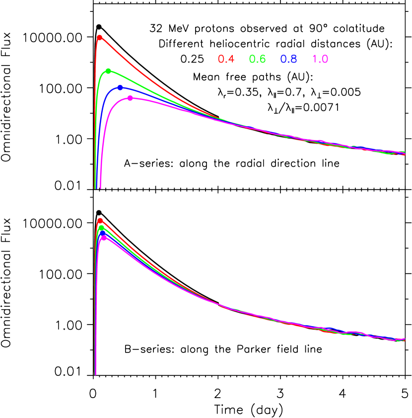
Figure 3: Same as Figure 2 except the diffusion coefficients are set as: the radial mean free path $\lambda_{r}=0.35$ AU (corresponding to the parallel mean free path $\lambda_{\parallel}=0.7$ AU at 1 AU), the perpendicular mean free paths $\lambda_{x}=\lambda_{y}=\lambda_{\perp}=0.005$ AU, and consequently, the ratio $\lambda_{\perp}/\lambda_{\parallel}=0.005/0.7=0.0071$ at 1 AU. The SEP “flood” (previously “reservoir”) phenomenon is reproduced in the simulations.

Figure 3 shows the simulation results of intensity-time profiles of $32$ MeV protons with the diffusion coefficients as follows: the radial mean free path $\lambda_{r}=0.35$ AU (corresponding to the parallel mean free path $\lambda_{\parallel}=0.7$ AU at 1 AU), the perpendicular mean free paths $\lambda_{x}=\lambda_{y}=\lambda_{\perp}=0.005$ AU, and consequently, the ratio $\lambda_{\perp}/\lambda_{\parallel}=0.005/0.7=0.0071$ at 1 AU. Other parameters and conditions are the same as Figure 2. In Figure 3, we can see that the SEP intensity observed at a smaller radial distance is higher than that observed at a larger radial distance. In other words, the SEP intensity decreases with increasing radial distance. The filled circles with different colors on the intensity-time profiles indicate the peak intensities of the SEP events. In addition, the SEP “flood” (previously “reservoir”) phenomenon is reproduced in the simulations.

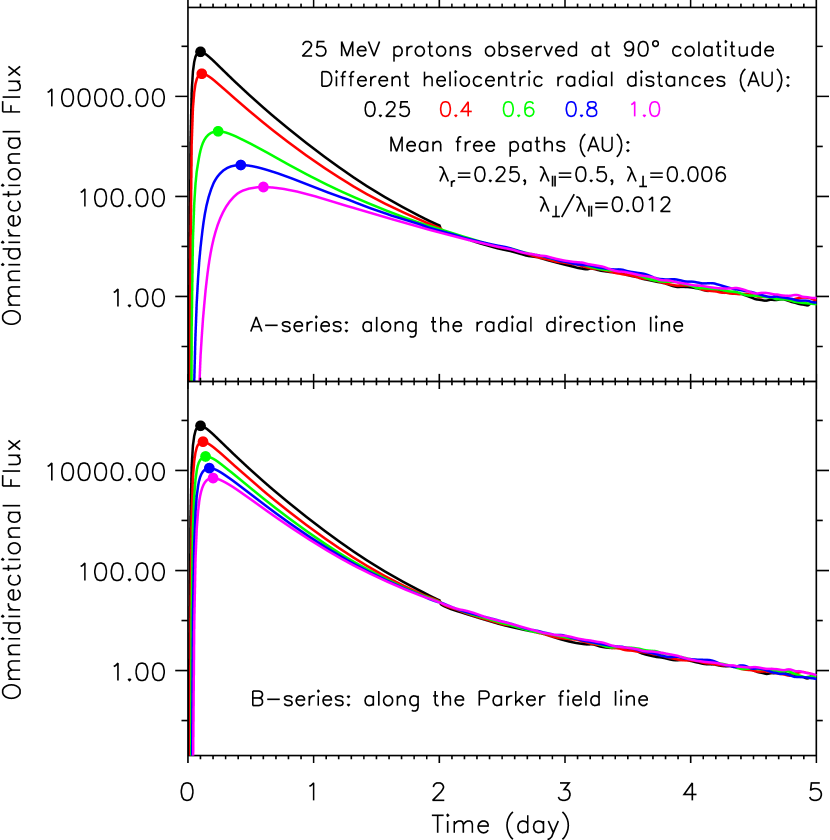
Figure 4: Same as Figure 2 except for $25$ MeV protons and the diffusion coefficients are set as: the radial mean free path $\lambda_{r}=0.25$ AU (corresponding to the parallel mean free path $\lambda_{\parallel}=0.5$ AU at 1 AU), the perpendicular mean free paths $\lambda_{x}=\lambda_{y}=\lambda_{\perp}=0.006$ AU, and consequently, the ratio $\lambda_{\perp}/\lambda_{\parallel}=0.006/0.5=0.012$ at 1 AU. The SEP “flood” (previously “reservoir”) phenomenon is reproduced in the simulations.

Figure 4 displays the simulation results of intensity-time profiles of $25$ MeV protons with the diffusion coefficients as: the radial mean free path $\lambda_{r}=0.25$ AU (corresponding to the parallel mean free path $\lambda_{\parallel}=0.5$ AU at 1 AU), the perpendicular mean free paths $\lambda_{x}=\lambda_{y}=\lambda_{\perp}=0.006$ AU, and consequently, the ratio $\lambda_{\perp}/\lambda_{\parallel}=0.006/0.5=0.012$ at 1 AU. Other parameters and conditions are the same as Figure 2. Similar to the results shown in Figure 2 and Figure 3, we can see that for both alignment scenarios of spacecraft (“A-series” in upper panel and “B-series” in lower panel), the SEP intensity decreases with increasing radial distance. The filled circles on the intensity-time profiles denote the peak intensities of the SEP events. During the late phases of SEP events, the SEP “flood” (previously “reservoir”) phenomenon is clearly reproduced.

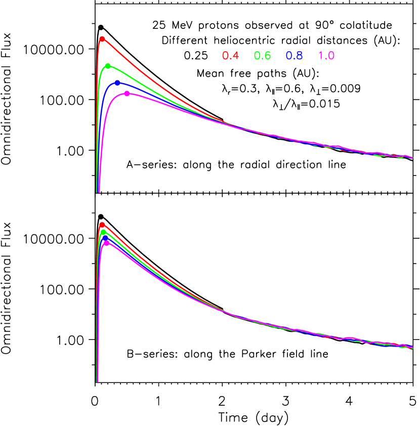
Figure 5: Same as Figure 4 except the diffusion coefficients are set as: the radial mean free path $\lambda_{r}=0.3$ AU (corresponding to the parallel mean free path $\lambda_{\parallel}=0.6$ AU at 1 AU), the perpendicular mean free paths $\lambda_{x}=\lambda_{y}=\lambda_{\perp}=0.009$ AU, and consequently, the ratio $\lambda_{\perp}/\lambda_{\parallel}=0.009/0.6=0.015$ at 1 AU. During the late phases, the SEP “flood” (previously “reservoir”) phenomenon is reproduced.

Figure 5 shows the numerical simulation results of intensity-time profiles of $25$ MeV protons with the diffusion coefficients as: the radial mean free path $\lambda_{r}=0.3$ AU (corresponding to the parallel mean free path $\lambda_{\parallel}=0.6$ AU at 1 AU), the perpendicular mean free paths $\lambda_{x}=\lambda_{y}=\lambda_{\perp}=0.009$ AU, and consequently, the ratio $\lambda_{\perp}/\lambda_{\parallel}=0.009/0.6=0.015$ at 1 AU. Other parameters and conditions are the same as Figure 4. As one can see in Figure 5, the SEP intensity decreases with increasing radial distance. We note that the filled circles on the intensity-time profiles denote the peak intensities of the corresponding SEP cases. During the late phases, the SEP “flood” (previously “reservoir”) phenomenon is reproduced.

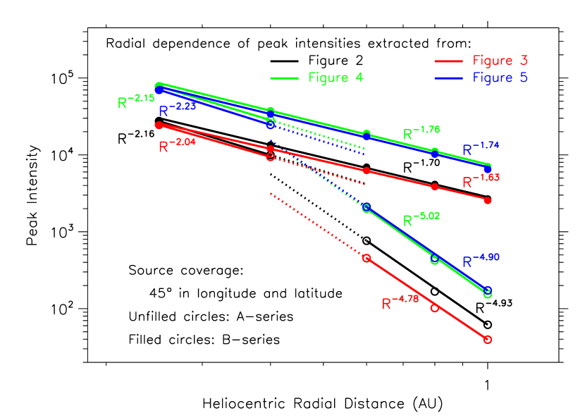
Figure 6: Radial dependence of the SEP peak intensities extracted from Figures 2 (black), 3 (red), 4 (green), and 5 (blue). The unfilled circles denote the peak intensities of the SEP events observed along the radial direction line, and the filled circles denote the peak intensities of the SEP events observed along the Parker magnetic field line. Note that the SEP source is $45^{\circ}$ wide in longitude and latitude. The functional form $R^{-\alpha}$ with different values of $\alpha$ denotes the modelling results of the corresponding SEP cases. A two-phase phenomenon is found in the radial dependence of the SEP peak intensities. The “position” of the breakpoint between the two phases depends on the magnetic connection status of the observers.

We extract the information of the peak intensities and the relevant radial distances of the SEP cases in Figures 2, 3, 4, and 5. We present this important information in Figure 6. The black, red, green, and blue circles and curves in Figure 6 denote the simulation results of SEP peak intensities extracted from Figures 2, 3, 4, and 5, respectively. In previous observational studies, a power-law function $I_{max}(R)=kR^{-\alpha}$, where $k$ is a constant, is usually used to model the radial dependence of the SEP peak intensities. Following the previous works, we model the radial dependence of the SEP peak intensities shown in Figures 2, 3, 4, and 5 with the functional form $I_{max}(R)=kR^{-\alpha}$. In Figure 6, the unfilled circles denote the peak intensities of the “A-series” SEP cases, i.e., those events observed along the radial direction line. The filled circles denote the peak intensities of the “B-series” SEP cases, i.e., those events observed along the Parker magnetic field line. The functional form $R^{-\alpha}$ with different values of $\alpha$ near the corresponding SEP cases denotes the modelling results of the radial dependence of the SEP peak intensities. As we can see, the peak particle intensities in the SEP events exponentially decrease with the increasing radial distances. For the SEP events observed along the Parker magnetic field line (“B-series”), the values of $\alpha$ are roughly in the range $[1.6,1.8]$, with a median value of $1.7$. For the SEP events observed along the radial direction line (“A-series”), the values of $\alpha$ are generally larger than those in the “B-series” SEP events. Interestingly, a two-phase phenomenon is found in the radial dependence of the SEP peak intensities. For the two spacecraft at radial distances $R=0.25$ AU and $R=0.4$ AU, respectively, the values of $\alpha$ are roughly in the range $[2.0,2.2]$. For the three spacecraft at radial distances $R=0.6$ AU, $R=0.8$ AU, and $R=1.0$ AU, respectively, the values of $\alpha$ are roughly in the range $[4.8,5.0]$. We note that the magnetic footpoints of the former two spacecraft are located inside the SEP source, while the magnetic footpoints of the latter three spacecraft are located outside the SEP source. This is why the value range $[2.0,2.2]$ of $\alpha$ determined from the former two spacecraft is relatively similar to the value range $[1.6,1.8]$ of $\alpha$ in the “B-series” SEP cases, but the value range $[4.8,5.0]$ of $\alpha$ determined from the latter three spacecraft is considerably different from the value range $[1.6,1.8]$ of $\alpha$ in the “B-series” SEP cases, where all of the five spacecraft’s magnetic footpoints are located at the center of the SEP source. The “position” of the breakpoint (transition point/critical point) between the two phases of the radial dependence of the SEP peak intensities depends on the magnetic connection status of the observers. In particular, the situation that whether the magnetic footpoint of the observer is located inside (even very near or on the boundary of source) or outside the SEP source is a crucial factor determining the value of the index $\alpha$. This finding suggests that a very careful examination of magnetic connection between SEP source and each spacecraft should be taken in the observational investigations to obtain an accurate estimate of the radial dependence of the SEP peak intensities. In addition, we find that the index $\alpha$ does not strongly depend on the energies of particles and the ratios of perpendicular to parallel diffusion coefficients, provided that the diffusion coefficients are relatively reasonable.

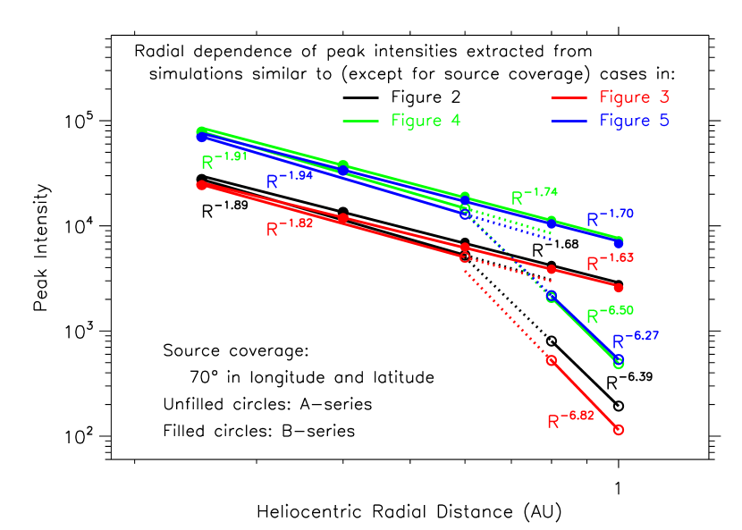
Figure 7: Same as Figure 6 except for the SEP source being $70^{\circ}$ wide in longitude and latitude. A two-phase phenomenon also exists in the radial dependence of the SEP peak intensities. The “position” of the breakpoint between the two phases depends on the magnetic connection status of the observers.

We also simulate the SEP cases with source width of $70^{\circ}$ in longitude and latitude. Figure 7 displays the simulation results and the modelling analyses of the radial dependence of the SEP peak intensities. The black, red, green, and blue circles and curves in Figure 7 denote the simulation results of the SEP cases similar to (except for the source coverage) the cases presented in Figures 2, 3, 4, and 5, respectively. We note that except for the source width, all of the other physical parameters and conditions of the simulations presented in Figure 7 are the same as those in Figure 6. The unfilled circles denote the peak intensities of the “A-series” SEP cases, and the filled circles denote the peak intensities of the “B-series” SEP cases. The functional form $R^{-\alpha}$ with different values of $\alpha$ near the corresponding SEP cases denotes the modelling results of the radial dependence of the SEP peak intensities. For the SEP events observed along the Parker magnetic field line (“B-series”), the values of $\alpha$ are roughly in the range $[1.6,1.7]$, which is similar to the value range $[1.6,1.8]$ indicated in Figure 6. For the SEP events observed along the radial direction line (“A-series”), the values of $\alpha$ are generally larger than those in the “B-series” SEP events. Similar to Figure 6, a two-phase phenomenon exists in the radial dependence of the SEP peak intensities. For the three spacecraft at radial distances $R=0.25$ AU, $R=0.4$ AU, and $R=0.6$ AU, respectively, the values of $\alpha$ are roughly in the range $[1.8,1.9]$. For the two spacecraft at radial distances $R=0.8$ AU and $R=1.0$ AU, respectively, the values of $\alpha$ are roughly in the range $[6.3,6.8]$. We note that the magnetic footpoints of the former three spacecraft are located inside the SEP source, while the magnetic footpoints of the latter two spacecraft are located outside the SEP source. This is why the value range $[1.8,1.9]$ of $\alpha$ determined from the former three spacecraft is similar to the value range $[1.6,1.7]$ of $\alpha$ in the “B-series” SEP cases, but the value range $[6.3,6.8]$ of $\alpha$ determined from the latter two spacecraft is considerably distinct from the value range $[1.6,1.7]$ of $\alpha$ in the “B-series” SEP cases. Because for the “B-series” SEP cases, the magnetic footpoints of all of the five spacecraft are located at the center of the SEP source. By combining Figure 6 and Figure 7, we can conclude that the “position” of the breakpoint (transition point/critical point) between the two phases of the radial dependence of the SEP peak intensities depends on the magnetic connection status of the observers in the heliosphere. Particularly, the situation that whether the magnetic footpoint of each observer is located inside (even very near or on the boundary of source) or outside the SEP source is a very important factor determining the value of the index $\alpha$. In this sense, the index $\alpha$ primarily depends on the physical properties (e.g., location, coverage) of the SEP sources and consequently on the longitudinal/latitudinal separations between the sources and the magnetic field line footpoints of the observers. Therefore, we suggest that a very careful examination of the magnetic connection between SEP source and each spacecraft should be taken in the observational studies to obtain an accurate estimate of the radial dependence of the SEP peak intensities. Additionally, we find that the index $\alpha$ does not strongly depend on the energies of particles and the ratios of perpendicular to parallel diffusion coefficients. In addition, we suggest that the function $R^{-1.7\pm 0.1}$, obtained in the “B-series” SEP cases, where all of the observers’ magnetic footpoints are located at the center of the SEP source, should be the lower limit for empirically modelling the radial dependence of the SEP peak intensities. For the SEP events similar to the “B-series” cases as shown in Figure 1, the value of index $\alpha$ does not strongly depend on the width of the SEP sources. These findings can be used to explain the majority of the previous empirical investigation results based on multispacecraft observations, and especially to reconcile the different/conflicting empirical values of index $\alpha$ in the literature.

4 Summary and Conclusions

SEPs have radiation effects and potential damages on space missions, and can risk the health of the astronauts working in space. To accurately estimate the potential radiation impacts of SEPs, it is very important to investigate the radial dependence of SEP intensities and fluences, particularly in the forthcoming era of Solar Probe Plus and Solar Orbiter. In this paper, we numerically solve the five-dimensional Fokker-Planck equation to investigate the radial dependence of SEP peak intensities in the inner heliosphere. The value of index $\alpha$ in the functional form $I_{max}(R)=kR^{-\alpha}$ is quantitatively determined in the simulations of various SEP scenarios. Two different styles of spacecraft alignment in the heliosphere are taken into account: (1) along the radial direction line (“A-series” cases in Figure 1); (2) along the nominal Parker magnetic field line (“B-series” cases in Figure 1). The main conclusions of our results in this paper are as follows:

1. The value of index $\alpha$ varies in a wide range, mainly depending on the physical properties (e.g., location, width) of SEP sources and consequently on the longitudinal/latitudinal separations between the sources and the magnetic field line footpoints of the observers. However, for the SEP events similar to the “B-series” cases, the value of $\alpha$ does not strongly depend on the width of the SEP sources.

2. The situation that whether the magnetic footpoint of the observer is located inside (even very near or on the boundary of source) or outside the SEP source is a crucial factor determining the value of index $\alpha$. A two-phase phenomenon is found in the radial dependence of the peak intensities in the “A-series” SEP cases. The “position” of the breakpoint (transition point/critical point) between the two phases of the radial dependence of the peak intensities depends on the magnetic connection status of the observers. We suggest that a very careful examination of the magnetic connection between SEP source and each spacecraft should be taken in the observational investigations to obtain an accurate estimate of the radial dependence of the SEP peak intensities.

3. We suggest that the function $R^{-1.7\pm 0.1}$, obtained in the “B-series” SEP cases, where all of the observers’ magnetic footpoints are located at the center of the SEP source, should be the lower limit for empirically modelling the radial dependence of the SEP peak intensities. In addition, the value of the index $\alpha$ does not strongly depend on the energies of particles and the ratios of perpendicular to parallel diffusion coefficients, provided that the diffusion coefficients are relatively reasonable.

4. The results provided in this paper can be used to explain the majority of the previous empirical results based on multispacecraft observations, and especially to reconcile the different/conflicting empirical values of index $\alpha$ in the literature. In addition, our findings can also be employed to predict and explain the observational results obtained from the two forthcoming spacecraft, i.e., Solar Probe Plus and Solar Orbiter.

In this work, we primarily pay attention to the simulations of the three-dimensional propagation of energetic protons in the inner heliosphere. In the future, we will investigate the radial dependence of intensities of electrons and heavy ions. The radial dependence of SEP fluences and radiation dosages is also a very interesting topic in the research field. We will also investigate the radial dependence of SEP intensities, SEP fluences, and radiation dosages in the outer heliosphere. In addition, in the future we will further investigate the radial and temporal evolution of the SEP events related to CME-driven shocks.

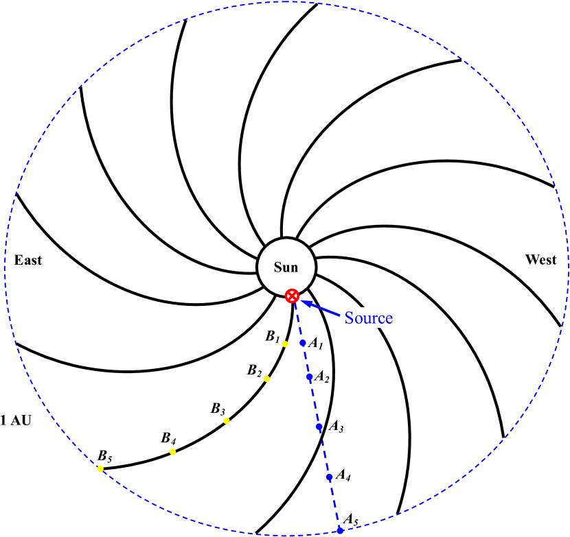
Figure 1: Diagram to show the alignment scenarios of the fleet of spacecraft in the heliosphere. The spacecraft fleet locations labelled with $A_{i}$ ($i=1,2,3,4,5$) are aligned along the radial direction line, and the spacecraft fleet locations labelled with $B_{i}$ ($i=1,2,3,4,5$) are aligned along the Parker magnetic field line connecting the SEP source. The heliocentric radial distances of spacecraft locations $A_{i}$ (also $B_{i}$) ($i=1,2,3,4,5$) are in sequence: $0.25$, $0.4$, $0.6$, $0.8$, and $1.0$ AU. Both the SEP sources and the fleet of spacecraft are located at $90^{\circ}$ colatitude.

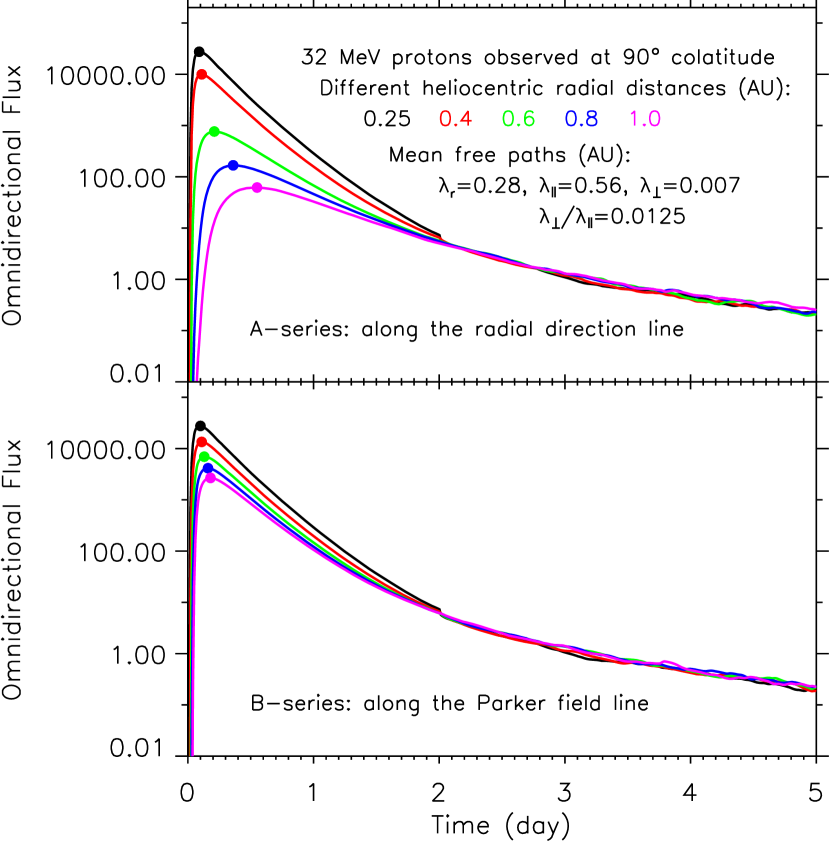
Figure 2: Simulation results of intensity-time profiles of $32$ MeV protons observed along the radial direction line (upper panel) and along the Parker magnetic field line (lower panel) originating from the SEP source. The SEP source is $45^{\circ}$ wide in longitude and latitude. The diffusion coefficients are set as: the radial mean free path $\lambda_{r}=0.28$ AU (corresponding to the parallel mean free path $\lambda_{\parallel}=0.56$ AU at 1 AU), the perpendicular mean free paths $\lambda_{x}=\lambda_{y}=\lambda_{\perp}=0.007$ AU, and consequently, the ratio $\lambda_{\perp}/\lambda_{\parallel}=0.007/0.56=0.0125$ at 1 AU. The curves with different colors denote the intensity-time profiles observed at different heliocentric radial distances: $0.25$, $0.4$, $0.6$, $0.8$, and $1.0$ AU. Note that the SEP “flood” (previously “reservoir”) phenomenon is reproduced in the simulations of a series of SEP cases with different radial distances. The filled circles with different colors on the intensity-time profiles indicate the peak intensities of the corresponding SEP cases.

References

- Aran et al. (2005) Aran, A., Sanahuja, B., & Lario, D. 2005, Ann. Geophys., 23, 3047
- Beeck & Wibberenz (1986) Beeck, J., & Wibberenz, G. 1986, ApJ, 311, 437
- Dröge et al. (2014) Dröge, W., Kartavykh, Y. Y., Dresing, N., Heber, B., & Klassen, A. 2014, J. Geophys. Res., 119, 6074
- Hamilton (1988) Hamilton, D. C. 1988, in Interplanetary Particle Environment (JPL Publ. 88-28; Pasadena: JPL), 86
- Hamilton et al. (1990) Hamilton, D. C., Mason, G. M., & McDonald, F. B. 1990, Proc. 21st Int. Cosmic Ray Conf., 5, 237
- He et al. (2011) He, H.-Q., Qin, G., & Zhang, M. 2011, ApJ, 734, 74
- He & Wan (2015) He, H.-Q., & Wan, W. 2015, ApJS, 218, 17
- He (2015) He, H.-Q. 2015, ApJ, 814, 157
- He & Wan (2017) He, H.-Q., & Wan, W. 2017, MNRAS, 464, 85
- Kallenrode (1997) Kallenrode, M.-B. 1997, J. Geophys. Res., 102, 22335
- Kozarev et al. (2010) Kozarev, K., Schwadron, N. A., Dayeh, M. A., et al. 2010, Space Weather, 8, S00E08
- Lario et al. (2006) Lario, D., Kallenrode, M.-B., Decker, R. B., et al. 2006, ApJ, 653, 1531
- Lario et al. (2007) Lario, D., Aran, A., Agueda, N., & Sanahuja, B. 2007, Adv. Space Res., 40, 289
- Lario & Decker (2011) Lario, D., & Decker, R. B. 2011, Space Weather, 9, S11003
- Lario et al. (2013) Lario, D., Aran, A., Gómez-Herrero, R., et al. 2013, ApJ, 767, 41
- Lario et al. (2014) Lario, D., Roelof, E. C., & Decker, R. B. 2014, ASP Conference Series, 484, 98
- McGuire et al. (1983) McGuire, R. E., van Hollebeke, M. A. I., & Lal, N. 1983, in Proc. 18th ICRC, vol. 10 (Bombay: Tata Institute of Fundamental Research), 353
- McKenna-Lawlor et al. (2005) McKenna-Lawlor, S. M. P., Dryer, M., Fry, C. D., et al. 2005, J. Geophys. Res., 110, A03102
- Parker (1965) Parker, E. N. 1965, Planet. Space Sci., 13, 9
- Reid (1964) Reid, G. C. 1964, J. Geophys. Res., 69, 2659
- Roelof et al. (1992) Roelof, E. C., Gold, R. E., Simnett, G. M., Tappin, S. J., Armstrong, T. P., & Lanzerotti, L. J. 1992, Geophys. Res. Lett., 19, 1243
- Rosenqvist (2003) Rosenqvist, L. 2003, Investigation of Radial Dependence of Gradual Solar Proton Flux Distribution (Tech. Memo. TOS-EMA/06-03)
- Rouillard et al. (2011) Rouillard, A. P., Odstricil, D., Sheeley, N. R., Jr., et al. 2011, ApJ, 735, 7
- Schlickeiser (2002) Schlickeiser, R. 2002, Cosmic Ray Astrophysics (Berlin: Springer)
- Shea et al. (1988) Shea, M. A., Smart, D. F., Adams, Jr., J. H., et al. 1988, in Interplanetary Particle Environment (JPL Publ. 88-28; Pasadena: JPL), 3
- Smart & Shea (2003) Smart, D. F., & Shea, M. A. 2003, Adv. Space Res., 31, 45
- Verkhoglyadova et al. (2012) Verkhoglyadova, O. P., Li, G., Ao, X., & Zank, G. P. 2012, ApJ, 757, 75
- Zhang et al. (2009) Zhang, M., Qin, G., & Rassoul, H. 2009, ApJ, 692, 109