On the absence of pulses from pulsars

A thesis submitted to the

Tata Institute of Fundamental Research, Mumbai
for the degree of Doctor of Philosophy
(in Physics)
by
Vishal Gajjar
National Centre for Radio Astrophysics
Tata Institute of Fundamental Research
Pune University Campus
Pune – 411 007
India
e-mail: vishalg@berkeley.edu
April, 2014

Synopsis

 
Thesis title : On the absence of pulses from pulsars
Vishal Gajjar
Supervisor : Dr. Bhal Chandra Joshi
 

Pulsars are one of the most fascinating objects in the known Universe. The very nature of their regular pulsation led to their discovery in the early days. They were the first to provide sound evidence about the existence of the neutron stars. In the last 47 years since the discovery of these objects, extensive research has been carried out to investigate the origin of the pulsar radiation. There have been many attempts to scrutinize the bright radio emission seen from pulsars by utilizing numerous observed phenomena. One of such phenomena is the rapid shape-changes in the observed single pulses in spite of their average profile showing remarkable stability for observations separated by decades. The sporadic nature of the single pulses provides important clues regarding the chaotic nature of the pulsar radiation. Thus, enormous amount of research have been focused on the modelling of the single pulses. There are different types of single pulse phenomena seen in the radio pulsar viz. drifting, nulling and mode-changing, which also shows interdependence in certain cases. Drifting and mode-changing has been modelled to some extent by many previous studies. However, nulling is one of the unexplained phenomena seen in the radio pulsars. The absence of emission in the individual single pulses has defied satisfactory explanation since its discovery 44 years ago.

Nulling in the radio pulsars has been reported by Backer (1970c) for the first time in four pulsars. Since its discovery, around 109 pulsars were reported to show prominent nulling behaviour in their single pulses. Nulling in pulsars has been historically quantified as the fraction of observed null pulses, also known as the nulling fraction (NF). In order to find the operating mechanism that causes only a few pulsars to exhibit noticeable nulling behaviour, NFs were compared with many pulsar parameters by various groups Ritchings (1976); Rankin (1986); Biggs (1992); Vivekanand (1995); Wang et al. (2007). However, no strong correlation between the NF and any pulsar parameter has been reported to date. Ritchings (1976) has reported that if the pulsar period is long, it is likely to have high nulling fraction compared to short period pulsars. As the period of the pulsar is directly related to its characteristic age, Ritchings (1976) speculated that pulsars die with increasing fraction of nulls in them. Contrary to that, Rankin (1986) presented an alternative hypothesis of correlation with the profile classes, where no dependence was noticed between NF and age of the pulsar in a similar profile morphological class. It was extensively shown in a study of around 60 pulsars, that the nulling fraction is likely to be less than 1% in pulsars exhibiting core component, while, it is more likely to have higher nulling fraction in pulsars exhibiting conal profile Rankin (1986). In a separate study by Biggs (1992), NF was confirmed to show correlation with the profile classes along with a few weak correlations. However, Wang et al. (2007) has shown that nulling does not show correlation with profile morphological classes as profiles with almost all classes show similar nulling behaviour. Moreover, Wang et al. (2007) suggested that nulling is an extreme form of mode-changing phenomenon. Thus, there is no common agreement between different studies regarding the true nature of any correlation.

The degree and form of pulse nulling varies from one pulsar to another. On one hand, there are pulsars such as PSR B0826$-$34 Durdin et al. (1979) which null most of the time, and PSR J1752+2359 Lewandowski et al. (2004), which exhibits no radio emission for 3 to 4 minutes. In contrast, pulsars such as PSR B0809+74 show a small degree of nulling Lyne & Ashworth (1983). Pulse nulling is frequent in pulsars such as PSR B1112+50, while it is very sporadic in PSR B1642$-$03 Ritchings (1976). Moreover, the pulsed emission abruptly declines by more than two orders of magnitudes during these nulls Lyne & Ashworth (1983); Vivekanand & Joshi (1997), which are as yet not well understood. While nulling pulsars have been known for last three decades, the recently discovered new class of sources, such as Rotating Radio transients McLaughlin et al. (2006); Keane & McLaughlin (2011); Burke-Spolaor et al. (2012) and intermittent pulsars Kramer et al. (2006); Camilo et al. (2012); Lorimer et al. (2012), also show a behaviour similar to classical nullers and are increasingly believed to be nulling pulsars Burke-Spolaor et al. (2012), indicating that nulling occurs in a significant fraction of pulsar population.

Pulsar emission at different radio frequencies, originates at different locations in the pulsar magnetosphere Komesaroff (1970). There are very few long simultaneous observations of nulling pulsars reported so far in the literature. In a simultaneous single pulse study of two pulsars, PSRs B0329+54 and B1133+16 at 327 and 2695 MHz, Bartel & Sieber (1978) showed highly correlated pulse energy fluctuations. Simultaneous observations of PSR B0809+74 for about 350 pulses indicated that only 6 out of 9 nulls were simultaneous at 102 and 408 MHz (Davies et al. 1984). About half of nulls were reported to occur simultaneously at 325, 610, 1400 and 4850 MHz for PSR B1133+16 (Bhat et al. 2007). In contrast, simultaneous nulls were reported at 303 and 610 MHz for PSR B0826$-$34 (Bhattacharyya et al. 2008). It is not clear if nulling represents a global failure of pulse radiation or is due to a shift in pulsar beam manifesting as lack of emission at the given observation frequency due to the geometry of pulse emission.

In light of all these previous investigations, long, sensitive, and preferably simultaneous observations at multiple frequencies of a carefully selected sample of pulsars are motivated. Thus, the aim of this thesis is to quantify, model and compare nulling behaviour between different classes of pulsars to scrutinize the true nature of the nulling phenomenon.

In this thesis, main results on three main investigations are discussed with the necessary background for each of them. In Chapter 1, basic introduction to the pulsars is provided. Details regarding the structure of the pulsar surroundings and origin of the radio emission are briefly derived in Chapter 2. Observations conducted for each investigation, are summarised with necessary details in Chapter 3. Further three chapters discuss results on the individual study. Chapter 4 presents results on the survey of nulling pulsar conducted using the GMRT. A comparison study between two high nulling fraction pulsars are discussed in Chapter 5. Unique simultaneous multi-frequency observations of two pulsars are summarised in Chapter 6. Chapter 7 presents summary of all the obtained results in the thesis along with a comprehensive view about the nulling behaviour suggested by our observations.

The chapter wise summary of this thesis is given below. First three chapters provide necessary background, along with the details regarding various observations.

Introduction

Introduction to pulsars, including their discovery and peculiar observed properties, are discussed in Chapter 1. A simple pulsar toy model is presented to explain the pulsating nature of this source. Radio waves from the pulsar, travelling through the interstellar medium, undergo numerous propagation related effects. A few of these effects can reduce the pulse energy to zero level. These effects could imitate intrinsic phenomenon like pulsar nulling. Thus, they are briefly explained to highlight their true nature. Different observed pulsar parameters and their stability on various time-scales are also discussed in the chapter. Various single pulse phenomena reported in the thesis are briefly introduced with examples.

Chapter 2 aims to provide necessary background about the currently known radio emission mechanism physics of the pulsars. It starts with a discussion on the structure of the neutron star along with the properties and composition of its surface, which were used to build the standard pulsar emission model proposed by Ruderman & Sutherland (1975). Origin of the coherent radio emission due to the growth in the two stream instability is briefly reviewed. This chapter also summarises, in detail, all previous studies conducted to investigate pulsar nulling phenomena. Different models proposed over the years to explain the mode-changing phenomenon are also listed in this chapter to relate them to pulse nulling in extreme conditions. Towards the end, primary incentives for the work reported in this thesis are listed in order to assess these models.

Details regarding all observations, reported in this thesis, are discussed with full details in Chapter 3. Justification regarding the selections of sources and observing frequencies for different objectives are elaborated in this chapter. In this thesis, observations from four different telescopes has been reported viz. the GMRT, the WSRT, the Arecibo telescope and the Effelsberg radio telescope. Details about all these telescopes are highlighted in this chapter including various local setting which were executed during the time of observations. Details about initial and basic analysis procedures followed for all our observations in this thesis work are also elaborated. These include, (a) obtaining single pulses from different observatories, (b) eliminating radio frequency interferences related effects, (c) estimation of the NF and (d) obtaining the null and burst length histograms from the separated null and burst pulses. A novel approach to isolate weak burst pulses among the null pulses is also introduced here for the first time.

Survey of nulling pulsars using the GMRT
(Gajjar, V., Joshi B. C. and Kramer M., 2012, MNRAS, 424, 1197)

In recent years Parkes Multibeam Survey (PKSMB) has discovered many new pulsars. Several of them show nulling behaviour in their discovery plots. We have carefully looked through the discovery plots of many pulsars, out of which, 5 promising candidates were selected for longer observations with the GMRT. In Chapter 4, the nulling behaviour of 15 pulsars, which include 5 PKSMB pulsars with no previously reported nulling behaviour, with the estimates on their NFs is reported. For four of these 15 pulsars, only an upper/lower limit was previously reported. The estimates of reduction in the pulsed emission is also presented for the first time in 11 pulsars. NF value for individual profile component is also presented for two pulsars in the sample viz. PSRs B2111+46 and B2020+28. Possible mode changing behaviour is suggested by these observations for PSR J1725–4043, but this needs to be confirmed with more sensitive observations. An interesting quasi-periodic nulling behaviour for PSR J1738–2330 is also reported.

We find that the nulling patterns differ between PSRs B0809+74, B0818–13, B0835–41 and B2021+51, even though they have similar NF of around 1%. We showed this by comparing the null length and burst length distributions using a two sample Kolmogorov-Smirnov test. Our results confirm that NF probably does not capture the full detail of the nulling behaviour of a pulsar. Thus, it can be speculated that, due to this, earlier attempts failed to correlate NF with various pulsar parameters.

We carried out the Wald-Wolfowitz runs test for randomness to 8 more pulsars. We find that this test indicates that occurrence of nulling, when individual pulses are considered, is non-random or exhibits correlation across periods. This correlation groups pulses in null and burst states, which was also noted by Redman & Rankin (2009). However, the durations of the null and the burst states shown to be modelled by a stochastic Poisson point process suggesting that these transitions occur at random. Thus, the underlying physical process for nulls in the 8 pulsars studied appears to be random in nature producing nulls and bursts with unpredictable durations. Moreover, modelling of the null length and the burst length distributions provided typical nulling and burst timescale (i.e. $\tau_{n}$ and $\tau_{b}$ respectively), which were derived for 8 pulsars for the first time to the best of our knowledge.

On the long nulls of PSRs J1738$-$2330 and J1752+2359
(Gajjar, V., Joshi B. C., and Geoffrey W. 2014a, MNRAS, 439, 221)

A detailed study of pulse energy modulation in two pulsars, PSR J1738$-$2330 and PSR J1752+2359, with similar NF has been presented in Chapter 5. The NFs were estimated to be 85$\pm$2% and 81% for PSR J1738$-$2330 and PSR J1752+2359 respectively. The aim of this study was to investigate similarity and differences between two high NF pulsars.

Both the pulsars exhibit similar bunching of the burst pulses classified as the bright phases, which are separated by long null phases. A similar quasi-periodic switching between these two state is observed for both the pulsars. However, using a new technique of pair-correlation-function (PCF), we have reported significant differences between these two pulsars. The PCF for PSR J1738$-$2330 indicates that the mechanism responsible for bright phases is governed by two quasi-periodic processes with periodicities of 170 and 270 pulses, On the other hand, the nulling pattern of PSR J1752+2359 is dominated by 540 pulse quasi-periodicity, which jitters from 490 to 595 pulses. These processes are not strictly periodic, but retain a memory longer than 2000 pulses for PSR J1738$-$2330, while the memory of PSR J1752+2359’s periodic structure is retained for only about 1000 periods.

Towards the end of each bright phase of PSR J1752+2359, an exponential decline in the pulse energy is reported. PSR J1738$-$2330 also shows similar exponential decay along with a flickering emission characterized by short frequent nulls towards the end of each bright phase. We modelled the bright pulse energy decay for PSR J1752+2359 and estimated their average lengths. A strong anti-correlation was found between the peak energy and the decay time for all bright phases in this pulsar. We demonstrated that the area under each bright phase is similar, suggesting that the energy release during all such events is approximately constant for PSR J1752+2359. The first bright phase pulse profile and the last bright phase pulse profile show striking differences between both the pulsars, hinting differences in transition from null phase to burst phase and vice-versa between the two pulsars. We report, for the first time, peculiar weak burst pulses during the long null phases of PSR J1752+2359, which we call as inter-burst pulses (IBPs). The IBPs are similar to emission seen from RRATs. The occurrence rate of the IBPs is random and uncorrelated with the preceding or following bright phase parameters. The polarization profiles for PSR J1752+2359 obtained from observations with the Arecibo telescope are reported for the first time. The total intensity and the circular polarization profiles of IBPs are slightly shifted towards the leading side compared to the conventional integrated profile, indicating a change in the emission region. No such pulses were seen in the long null phases of PSR J1738$-$2330. Lastly, we do not observe any GPs in our long observations unlike such pulses being reported at low frequencies in PSR J1752+2359 Ershov & Kuzmin (2005). Hence, these results confirm that even though these two pulsar have similar but significantly high NFs, they show very different nulling behaviour.

Simultaneous multi-frequency study of pulse nulling behaviour in two pulsars
(Gajjar, V., Joshi B. C., Kramer M., Smith R. and Karuppusamy R., 2014b, ApJ, 797, 18)

A detailed study on the simultaneous occurrence of the nulling phenomena in two pulsars, PSRs B0809+74 and B2319+60, is reported in Chapter 6. The observations were conducted simultaneously at four different frequencies, 313, 607, 1380 and 4850 MHz, from three different telescopes viz. the GMRT, the WSRT and the Effelsberg radio telescope. The overlap time for each pulsar was around 6 hours between different observatories.

We obtained single pulses at each frequency and the on-pulse energies were compared across all four frequencies, which showed remarkable similarity in the pulse energy fluctuations for both the pulsars. To quantify these similarities, we obtained the NF at each frequency which were found to be consistence within the error bars, at all four frequencies for both the pulsars. Similarly, the one-bit sequences were also compared using the contingency table analysis. To measure the statistical significance of the contingency tables, we measured the Cramer-V and the uncertainty coefficient for each pair of frequencies. For PSR B0809+74, both the statistical tests showed highly significant broadband nulling behaviour. For PSR B2319+60, the significance was marginally lower for the pairs involving 4850 MHz.

We also scrutinize all the nonconcurrent pulses (i.e. pulses which did not show similar emission states across different frequencies) for both the pulsars to investigate their true nature. For PSR B0809+74, we found that out of 12 nonconcurrent pulses, 7 (about 58%) occurred at the transition point where emission state is switching from null to burst (or vice-verse). Similarly for PSR B2319+60, we found that out of 158 nonconcurrent pulses, 82 (about 52%) occurred at the transition point where emission state is switching. Thus, both pulsars showed remarkable similarity in the overall broadband behaviour, also accounting the fraction of nonconcurrent pulses at the transition points.

A slight difference can be seen for the exclusive pulse profiles, pulses which exclusively occurred at a single observing frequency, between both the pulsars. PSR B0809+74 showed significantly narrow pulses (except at 4850 MHz) aligning the overall pulse profile, while PSR B2319+60 showed significantly weak pulses which are shifted towards the leading edge compared to the overall pulse profile. However, a strong claim can not be made regarding their true shapes, due to their small numbers. We also compared the null length and the burst length distributions across all observed frequencies which showed similar distribution with high significance ($>$99%) for both the pulsars. These results clearly suggest that nulling is truly a broadband phenomena. It favours models invoking magnetospheric changes on a global scale compared to local geometric effects as a likely cause of nulling in these pulsars.

Conclusions

Final summary of all obtained results are listed in Chapter 7 and their implications are discussed. We have also combined the obtained results on three different aspects of the nulling behaviour. In light of these results, following interpretations about the nulling phenomena can be suggested.

1. NF is not an ideal parameter to quantify nulling behaviour, confirmed firmly by comparing low NF pulsars as well as high NF pulsars.

2. Nulling occurs randomly with unpredictable length durations. Quasi-periodicities seen in the high NF pulsars can also be explained by the Markov models with a forcing function.

3. Nulling is an extreme form of mode-changing phenomena which occurs on a global magnetospheric scale.

4. Geometric reasons are less favoured as a likely cause of nulling phenomena due to the randomness and broadband behaviour reported in this thesis.

These results can also be extended to explain the peculiar emission behaviour seen in the intermittent pulsars and the RRATs. Future work motivated by these observations are listed towards the end of this chapter.

List of publications

Refereed Journal

• Gajjar, V., Joshi B. C. and Kramer M., 2012,
  Survey of nulling pulsars using the Giant Meterwave Radio Telescope,
  MNRAS, 424, 1197

• Gajjar, V., Joshi B. C., and Geoffrey W. 2014a,
  On the long nulls of PSRs 11738-2330 and J1752+2359,
  MNRAS, 439, 221

• Gajjar, V., Joshi B. C., Kramer M., Smith R. and Karuppusamy R., 2014b,
  Frequency independent quenching of pulsed emission,
  ApJ, 797, 18

Proceedings

• Gajjar, V., Joshi B. C. and Kramer M., 2009,
  Peculiar nulling in PSR J1738-2330,
  ASP conference series, 407, 304

• Gajjar, V., Joshi B. C. and Kramer M., 2012,
  Broadband nulling behaviour of PSR B2319+60,
  ASP conference proceeding, 466, 79

• Gajjar, V., Joshi B. C. and Kramer M., 2013,
  A survey of nulling pulsars using the Giant Meterwave Radio Telescope,
  Proceedings of IAU Symposium, 291, 385

• Gajjar, V., Joshi B. C. and Kramer M., 2011,
  A survey of nulling pulsars using GMRT,
  Astronomical Society of of India Conference Series, 3, 118

Chapter 1 Introduction

Pulsating stars (aka Pulsars) are one of the most exotic objects in the known Universe due to their unique nature. Pulsars are highly magnetised rotating neutron stars. They emit beams of radiation in a concentrated emission cone which sweeps the surrounding sky in a light-house manner. When this beam of radiation crosses the line-of-sight towards the observer, a pulse can be detected. This train of pulses has a unique period associated with it, which is the period of rotation of the pulsar. Pulsars are known to emit radiation from radio to gamma-rays frequency regime, although from widely spaced emitting regions with different emission mechanisms. However, this thesis particularly focuses on the study in the radio frequency regime only.

1.1 Pulsar Discovery

The first pulsar was discovered serendipitously in the late 1960s Hewish et al. (1968). Jocelyn Bell, a graduate student from the Cambridge University, and her supervisor Anthony Hewish, were conducting experiments to study the interplanetary scintillations. During these investigations, a train of pulses was detected. In an interesting account by Bell-Burnell (1977), the first ever recorded signal from a pulsar was noticed as “a bit of scruff” on a chart recorder. The observed train of pulses, with 1.33 second periodicity, were first thought to be terrestrial signal. However, regular appearance of this signal following the sidereal time, eliminated the possibility of terrestrial origin (the source was subsequently named CP 1919 which is now known as pulsar B1919+21). All different possibilities were considered, including a possible beacon from an extra-terrestrial intelligence civilization. However, after a few months of this discovery, couple of more such sources were found at different locations in the sky, making it clear that the recorded phenomena has a natural origin. The peculiar property of such short periodicity allowed Hewish et al. (1968) to conclude that, compact objects such as white dwarfs and neutron stars could be the possible source. The suggestion that pulsars are rotating neutron stars was also provided by Gold (1968). This was indeed confirmed later when a pulsar with 33 millisecond periodicity was discovered powering the Crab nebula, which is a supernovae remnant Pacini (1968).

The existence of neutron star in a stellar life cycle was first predicted by Baade & Zwicky (1934). However, a possible detection of any signal from the neutron stars was never expected. Hence, the discovery of radio signals from pulsars became the single most significant event to prove the existence of neutron stars. Currently, more than 2000 pulsars are known which exhibit a plethora of observed phenomena. Pulsars are fantastic laboratory to test many physical and astrophysical problems. They were extensively used to study the interstellar medium. Pulsars are also proposed to be an important probe in the gravitational wave detection [see Joshi (2013) for a review].

1.2 Pulsar Toy model

Pulsar radio emission have been studied extensively to scrutinize the emission mechanism. The radio emission was found to be highly polarized. In an interesting study by Radhakrishnan & Cooke (1969), pulsar emission was shown to be originating near the magnetic field lines. The rotating vector model suggests, pulsar has a co-rotating radiation beam aligned with its magnetic axis. The angle between the rotation axis and the magnetic axis, also known as $\alpha$, produces pulsed radio emission (shown in Figure 1.1) every time the radiation beam sweeps the line-of-sight of the earth Radhakrishnan & Cooke (1969). This picture of the pulsar toy model is shown in Figure 1.2.

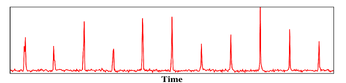
Figure 1.1.: An observed train of pulses from PSR B0809+74 (here PSR stands for Pulsating Source of Radio and the number followed by it presents right-ascension and declination of the source)

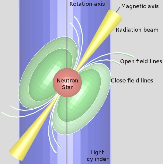
Figure 1.2.: The schematic diagram of a radio pulsar to illustrate various regions around the neutron star (not to scale). The magnetic axis is misaligned with the rotation axis, which gives the peculiar pulsating properties to each pulsar. The field lines enclosing inside the light cylinder are classified the close field line region while the field lines which cross the light cylinder belong to open field line region (cartoon using the free 3D modeling package : blender www.blender.org).

The charged particles, bound to the magnetic field lines, are forced to corotate with the neutron star. However, as the distance from the neutron star rotation axis increases, the linear velocity of the rotation of the charge particles also increases up to speed of light. Beyond this boundary, the particles can not continue to corotate with the star. This boundary, also known as the light cylinder, divides the pulsar magnetosphere in two different regions, namely the open field lines and the close field lines as illustrated in Figure 1.2. The region of open field lines allows the charge particles to accelerate and escape the magnetosphere. The radio emission is generated inside this open field line regions. The details regarding the production of the radio emission is given in Section 2.1.4.

1.3 Propagation of radio waves

The radio waves generated by the pulsar pass through the Galactic interstellar medium (ISM) before reaching the observer. During their travel, the signal experiences multiple propagation effects, such as dispersion, scattering and scintillation, discussed below. Some of these effects can be reverted to retrieve the original signal.

1.3.1 Pulse dispersion

The ionised component of the interstellar medium disperses the passing signal by introducing a frequency dependent delay. Pulse at higher frequencies experiences relatively shorter delay compared to pulse at lower frequencies. The delay in pulse arrival times across a finite bandwidth can be seen in Figure 1.3.

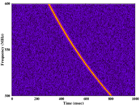
Figure 1.3.: Pulse dispersion shown for a simulated pulsar, with period of around 1 sec and DM of 100 pc cm^-3. The expected delay across the observed bandwidth of 100 MHz at 550 MHz is around half the pulsar period.

Quantitatively, the delay, $\bigtriangleup{\tau}$ in arrival times between a high frequency, $f_{high}$, and a low frequency, $f_{low}$, can be given as Lorimer & Kramer (2004),

$$\bigtriangleup{\tau}~{}=~{}4.15~{}\times~{}\bigg{[}\bigg{(}\frac{f_{low}}{GHz}\bigg{)}^{-2}~{}-~{}\bigg{(}\frac{f_{high}}{GHz}\bigg{)}^{-2}\bigg{]}~{}\times~{}\bigg{(}\frac{DM}{pc~{}cm^{-3}}\bigg{)}~{}msec.$$ (1.1)

Here the dispersion measure (DM), which is an integrated column density of electrons, can be calculated as,

$$DM~{}=~{}\int_{0}^{d}{n_{e}}dl~{}~{}pc~{}{cm^{-3}}.$$ (1.2)

Here, d is the distance to the pulsar and $n_{e}$ is the electron density of the ISM. For all the known pulsars, the DM can be measured very accurately by comparing the pulse delay between higher and lower frequency channels across the observed bandwidth (as seen in Figure 1.3). The model of the electron density, known as NE2001, across various line-of-sights has been approximately measured from independent estimates Cordes & Lazio (2002). Thus, DM of a pulsar also provides a good measure of its distance with $\sim$30% uncertainty.

The dispersion effects can easily be removed from the DM of the pulsar. The procedure to remove the dispersion smearing is known as the dedispersion. There are two different ways in which the dispersion can be reverted to retrieve the original signal (a) Incoherent dedispersion and (b) Coherent dedispersion. During the coherent dedispersion, a model of the ISM needs to be adapted to revert the phase delays. This procedure is generally carried out during the observation time itself. However, it is also possible to coherently dedisperse the recorded data as well. While, for the case of incoherent dedispersion, signals are delay compensated for individual frequency channels.

1.3.2 Pulse scattering

Scattering of the pulsar signals manifest as an exponential tail at the trailing edge of the received pulse. The irregularities in the electron density of the ISM results in a one-sided broadening of the pulse. To scrutinize the scattering phenomena, the intermediate ISM can be presented as multiple patches with varying refractive index in a thin screen. These patches perturbs the phase of the impinging radio wave-front, causing a scatter of the resultant signal. A simplified screen approximation of the ISM is shown in Figure 1.4, in which the multipath scattering can be seen at the observing end. Signals received by the observer from different patches arrive slightly later compared to signals that travelled unperturbed. Hence, an exponential tail can be observed once the leading phase of the pulse arrives.

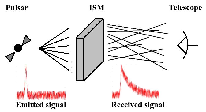
Figure 1.4.: A simplified model of the ISM screen approximation. The pulsar signal undergoes multipath scattering inside the ISM. The signals with different path lengths, refracted from different ISM regions, arrive at the telescope with varying delay time-scales. This effect causes the pulse to grow broader with an exponential tail at the trailing edge. [Figure adapted from an original version in Lorimer (2008)]

As can be seen from Figure 1.4, the signal to noise ratio (S/N) reduces substantially due to the scattering. If the scattering tail decay time-scales matches the pulsar period, pulse detection becomes a daunting task. The relation between the exponential decay time-scale, pulsar distance (d) and observing frequency (f) can be presented as Lorimer & Kramer (2004),

$$\tau_{s}~{}\propto~{}d^{2}~{}f^{-4}.$$ (1.3)

Lower frequencies show relatively longer tails due to the above given relation. Hence, most of the pulsar searches are conducted above 1 GHz. The ISM is also not uniform in different directions. The Galactic plan and specially the Galactic center are regions where the electron density highest and the line-of-sight passes through a longer path of electrons, making search for pulsars a more challenging task in these regions.

1.3.3 Pulse scintillation

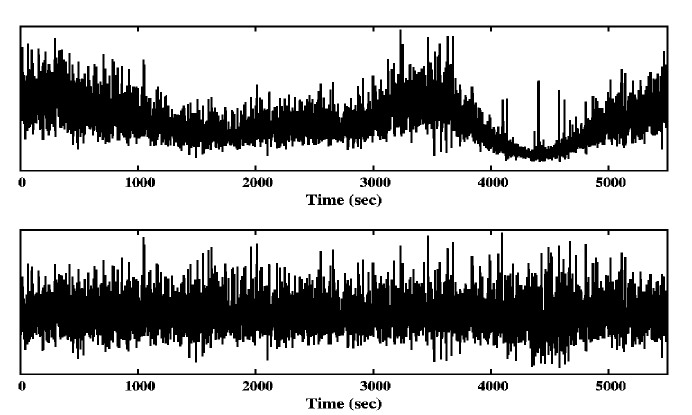
Figure 1.5.: The interstellar scintillation seen for the pulse peak intensities. The top panel shows the peak pulse intensity as a function of time. Note the gradual variations due to the changing interference pattern from the turbulent ISM. The bottom panel shows peak pulse energy after removal of the interstellar scintillation normalizing by the block averages.

Closely similar to the scattering phenomena, single pulses from the pulsars undergo large pulse intensity fluctuations. This effect is similar to the optical twinkling of stars caused by the Earth’s atmosphere. Figure 1.1 shows varying pulse intensities, a combination of intrinsic and scintillation effects seen for all known pulsars. It was first reported by Lyne & Rickett (1968). The pulse scintillation is caused by the highly turbulent and inhomogeneous ISM Scheuer (1968). Different ISM patches, as mentioned in the Section 1.3.2, also cause an interference pattern at the observer’s plane. Due to the relative motion between the observer, the pulsar and the ISM patches, the interference pattern also moves across the observer’s plane. The relative velocity shifts the enhanced and the reduced intensity regions to cause changes in the pulse intensity. The time-scale of this intensity fluctuation depends upon the aggregated relative velocity Scheuer (1968). Scintillation can also reduce the observed pulse intensity to go below the detection threshold, making the single pulse study a challenging task. Scheuer (1968) has suggested that pulse scintillation are correlated only over a limited range of frequencies, also known as the scintillation bandwidth ($\bigtriangleup{f}$) related to the observing frequency ($f$) as, $\bigtriangleup{f}{~{}\propto~{}}f^{4}$. This matched well with the early observations of ten pulsars by Rickett (1969). The correlation bandwidth for different line-of-sights can be calculated using Galactic electron density model Cordes & Lazio (2002). Hence, by using a relatively larger bandwidth than $\bigtriangleup{f}$, scintillation effects can be reduced.

Figure 1.5 shows only the peak pulse energy of around 5000 consecutive burst pulses, of PSR B0809+74 observed from the Giant Meterwave Radio Telescope (GMRT) at 325 MHz with 33 MHz bandwidth. The gradual fall and rise in the pulse intensity is clearly evident. For an unbiased treatment of the individual pulses, pulse intensities can be averaged in consecutive blocks and each pulse can be normalized with their respective block average. The effective peak pulse intensities, normalized by their respective block average to remove the interplanetary scintillation effect, is also shown in Figure 1.5.

1.4 Observed pulsar parameters

1.4.1 Integrated profile

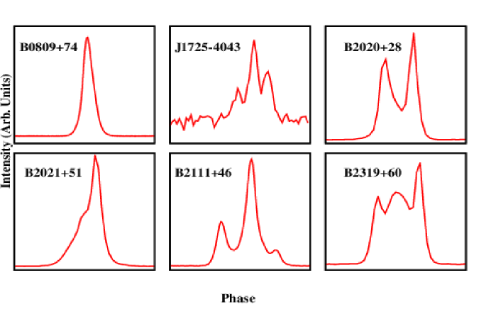
Figure 1.6.: Integrated profiles of six pulsars, observed from the GMRT at 325 MHz. Note the differences in the shape and structure between various profiles.

Pulsar exhibits varying types of fluctuations in the shape of the individual pulses. However, after adding many hundreds or a few thousand pulses, a stable shape can be obtained which is known as the integrated profile of the pulsar. The profile of a pulsar remains constant, at a given observing frequency, irrespective of the epoch of observations. The integrated profile is like a unique signature of the individual pulsar and it shows wide variety of shapes and structures across all known pulsars. A few such examples of integrated profiles, to highlight their different shapes, are shown in Figure 1.6. The remarkable stability of the integrated profile suggest a stable emission process for each pulsar. Hence, the study of the integrated profiles is important to map the radio emitting regions. However, a few pulsars show switch between different integrated profiles, a phenomena known as mode-changing, which tends to occur for a few hundred to a few thousand pulses (see Section 1.5.3 for details). There are also effects like geodetic precession which causes a gradual change in profile shapes, although number of pulsars, in which this effect is seen, are very few.

1.4.2 Period and slowdown

The period of the pulsar, which corresponds to its rotation, is one of the pulsar parameter measured with high accuracy. The period does show a gradual slow down due to the loss in the rotational kinetic energy of the neutron star with time. However, this slowdown of the period is only one part in 10¹⁵ second for normal pulsars. The slowdown of the pulsar, presented as $\dot{P}$ (= dP/dt), can be measured accurately to predict the period of the pulsar at each epoch of observations. As the gradual changes in the slowdown rate is related to the amount of energy release by the neutron star, young pulsars show higher slowdown rate compared to older pulsars. The rate of loss of rotation kinetic energy, the spin-down luminosity, can be presented as Lorimer & Kramer (2004),

$$\dot{E}~{}=~{}-\frac{dE_{rot}}{dt}~{}=~{}-\frac{d(I\varOmega^{2}/2)}{dt}~{}=~{}-I\varOmega\dot{\varOmega}~{}=~{}\frac{4\pi^{2}I\dot{P}}{P^{3}}.$$ (1.4)

Here, $I$ is the moment of inertia and $\varOmega~{}=~{}2\pi/P$ is the rotation angular frequency. For a normal pulsar with $P$ of 1 sec, $\dot{P}$ around 10^-15 s/s and $I$ of the order of $10^{45}~{}g~{}cm^{2}$ [assuming spherical shape with canonical values of mass around 1.4$M_{\odot}$ and radius of 10 km Lorimer & Kramer (2004)], the loss of rotational energy is of the order of 10³¹ ergs/sec. However, the radio luminosity of a pulsar is a significantly small fraction of this energy as most of the energy of the pulsar goes in the emission at X-rays and $\gamma$-rays frequencies along with the energy carried away by the particle winds and magnetic dipole emission.

Figure 1.7.: $P-\dot{P}$ diagram of around 2000 pulsars. Two cluster of points represent the normal and the millisecond pulsars population at their respective period range. A few points, extending from the normal pulsars population towards the upper right corner are the neutron stars discovered at higher energies. [The data were obtained from the www.atnf.csiro.au/research/pulsar/psrcat Manchester et al. (2005)]

$P$ and $\dot{P}$ are unique parameters which can also be used to calculate other parameters such as the characteristic age and the magnetic field. Pulsar exhibits wide range of periods, starting from the fastest known pulsar PSR J1748$-$2446ad with period of around 1.3 msec Hessels et al. (2006) to the slowest known pulsar PSR J2144$-$3933 with period of around 8.5 sec Manchester et al. (1996). Figure 1.7 shows the $P-\dot{P}$ diagram, obtained from around 2000 pulsars. The plot shows scatter of points with two loosely bound clusters with a bridge joining them. The clusters correspond to two main groups, which seem to show slightly different observational properties. Pulsars with period less than 30 msec belong to a special class known as the millisecond pulsars. They correspond to old neutron stars which have been ’recycled’ by phases of mass accretion from the binary companion, to radiate once again. The big cluster at relatively slow rotation rate, with periods between 0.1 to 1 sec, are the normal pulsars. In this thesis, radio emission properties of only the normal pulsars have been discussed.

1.4.3 Pulse Polarization

As mentioned in Section 1.2, pulsar signals are highly polarized. The plane of the linear polarization point towards the orientation of the magnetic field lines at the point of emission. Hence, pulse polarization measurements are useful to scrutinize the geometry of the radio emitting region. Using the radio observations, four Stokes parameters, I, Q, U and V can be obtained, where I is the total intensity of the signal, while V is the circular polarization intensity. The linear polarization intensity, obtained from Q and U profiles as L ($=\sqrt{Q^{2}+U^{2}}$), is also of great importance to investigate. Along with these parameters, it is also of interest to study the position angle (PA) of linear polarization (Equation 5.7) as a function of pulse phase.

$$PA~{}=~{}\frac{1}{2}{tan^{-1}\bigg{(}\frac{U}{Q}\bigg{)}}$$ (1.5)

The error in the PA can be measured as Mitra & Li (2004),

$$\bigtriangleup{PA}~{}=~{}\frac{\sqrt{(U\times\bigtriangleup{U})^{2}~{}+~{}(Q\times\bigtriangleup{Q})^{2}}}{2\times{L^{2}}}.$$ (1.6)

Here, $\bigtriangleup{U}$ and $\bigtriangleup{Q}$ are the root mean square deviations from Stokes U and Q average profiles respectively.

Radhakrishnan & Cooke (1969) has demonstrated that the emission in the radio regime originates near the magnetic pole, using the PA changes across the pulse profile. In the proposed Rotating-vector model, Radhakrishnan & Cooke (1969) demonstrated the expected shape of the PA angle changes as characteristic $S$-shape curve by simple geometric arguments. The expected polarization angle swing, as the line-of-sight cross the magnetic field lines, matched perfectly well with the observed PA swing for many pulsars. It should be noted that a few pulsar also exhibit an abrupt 90^∘ swing in the otherwise smooth $S$-shape curve. These kind of changes tend to occur due to the presence of two different orthogonal polarization modes. The change in their dominance can cause such abrupt swing of 90^∘. Figure 2 shows an example of different polarization profiles obtained for PSR B0525+21, along with the $S$-shaped PA swing across the pulse profile. In principle, the observed PA swing can also help to derive other pulsar parameters, such as $\alpha$ and $\beta$ using the geometry. Here, $\beta$ (also known as the impact angle) is an angle between the magnetic pole and the center of the line-of-sight cut on the emission beam measured away from the rotation axis. However, a degeneracy can occur between an outer line-of-sight cut (positive $\beta$) and an inner line-of-sight cut (negative $\beta$) for limited range of active pulse longitude Narayan & Vivekanand (1982).

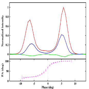
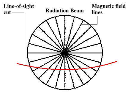
Figure 1.8.: Polarization profiles with the rotating vector model. (a) The panel shows different polarization profiles for PSR B0525+21 observed at 1.4 GHz [Archival data obtained from the EPN pulsar network; original observations by Gould & Lyne (1998)]. The total intensity is shown with red line while the linear and circular polarization profiles are shown with blue and green solid lines. The bottom panel shows the PA (magenta line) across the pulse longitude with the measured error bars. The characteristic $S$-shaped swing is clearly evident in the bottom panel. (b) The panel shows the top view of the radiation beam, with magnetic field lines emanating around the magnetic pole. The red line-of-sight cut is shown to trace the PA swing as it passes through magnetic field lines of changing orientation, highlighting the rotating vector model proposed by Radhakrishnan & Cooke (1969).

As the pulsar signal passes through the interstellar medium, it also undergoes Faraday rotation, which is a frequency dependent rotation of the polarization angle. The effect can cause artificial changes in the PA, although these changes are large and can easily be distinguished from the intrinsic PA changes. However, a careful calibration is required using an artificial source before obtaining the four Stokes parameters.

1.5 Single pulse phenomena

1.5.1 Giant Pulses

Pulsar in the Crab nebula was one of the first source discovered through its extremely strong burst pulses Staelin & Reifenstein (1968). These pulses, also known as the Giant pulses, have peak intensities up to 1000 times higher than normal individual pulses. Detail study of these Giant pulses from the Crab pulsar has revealed that they are superposition of extremely narrow nanosecond duration structures Hankins et al. (2003). Currently, giant pulses are known to occur in around 10 pulsars. They are mostly reported in the millisecond pulsars Kinkhabwala & Thorsett (2000); Romani & Johnston (2001); Joshi et al. (2004). They have also been reported in three regular pulsars Kuzmin & Ershov (2004); Ershov & Kuzmin (2005), only at lower frequencies of 100 MHz, which remain to be verified at higher frequencies. In the earlier studies Staelin & Reifenstein (1968); Kinkhabwala & Thorsett (2000); Joshi et al. (2004), it was reported that giant pulses have significantly smaller pulse widths compared to average pulses. The expected brightness temperature of these pulses reached up to 10³⁷ K, making them the brightest source in the known Universe Cordes et al. (2004). They also tend to occur near the edge (either near the trailing edge or near the leading edge) of the pulse profile. The emission mechanism behind the production of giant pulses, with this peculiar nature, still remain unidentified.

1.5.2 Drifting

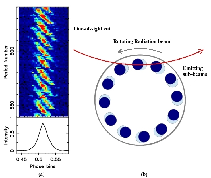
Figure 1.9.: An example of drifting subpulses in PSR B0809+74. (a) A stack of around 100 pulses are shown in the top panel with the average profile in the bottom panel, obtained from the GMRT observations at 325 MHz. Individual pulse intensities are shown with a color ramp from blue to red. Note the varying structure of individual pulses with two (sometimes three) subpulses. The drifting towards the leading side is clearly evident in the consecutive pulse sequence. (b) The rotating sub-beams carousal with a line-of-sight cut is shown to demonstrate the drifting of subpulses each time the line-of-sight cuts the radiation beam during each period. Two sets of sub-beams are shown (light blue and dark blue) to show the displacement of sub-beams during a period interval.

A few pulsars tend to show individual pulses with multiple peaks (i.e. subpulses), although the integrated profiles are smooth with single component in many cases. For such pulsars, contiguous pulses are reported to show marching of these subpulses across the pulse longitude, also known as the drifting. The drifting of the subpulses was first reported by Drake & Craft (1968). Figure 1.9(a) shows sequence of observed pulses from PSR B0809+74. The drifting of the subpulses is clearly evident here with a periodicity of around 11 periods after which the pattern repeats itself (see Section 2.2.2 for more details regarding the drifting periodicities). Ruderman & Sutherland (1975) have suggested the cause of the periodicity due to a rotating carousal of sub-beams within a hollow radiation beam (as shown in Figure 1.9(b)). Each time the line-of-sight passes across the radiation beam, it encounters a slightly different set of arrangements of the sub-beams because of their rotation around the magnetic pole. As these sub-beams are uniformly distributed, the patten repeats itself after certain number of periods as each sub-beam is replaced by an adjacent sub-beam. Deshpande & Rankin (2001) has proposed a method to determine the number of sub-beams in the rotating carousal.

The periodicity of the drifting subpulses is defined as $P_{3}$ while the separation between the subpulses in the individual pulse is defined as $P_{2}$. A significant correlation was reported between the $P_{3}$ and pulsar age Wolszczan (1980); Rankin (1986). However, in the largest survey conducted on the drifting pulsars Weltevrede et al. (2006, 2007); Weltevrede (2007), it was concluded that no such correlation exist. Drifting of subpulses can occur in both directions, from leading side to trailing side and vice-versa. Rankin (1986) has reported that pulsars do not have any preferred sense of drifting as equal number of pulsars were found exhibiting different drifting directions. Weltevrede et al. (2006, 2007) has also concluded that drifting is an intrinsic property of emission mechanism. However, for a few pulsars it is not possible to detect classical drifting behaviour because their subpulses are disordered. As pulsar gets older, the sub-beams structure becomes more and more organized to produce detectable subpulse drifting pattern Weltevrede et al. (2006, 2007).

1.5.3 Mode-changes

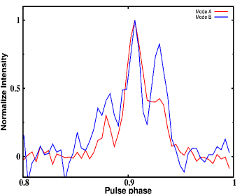
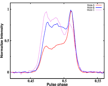
Figure 1.10.: Two examples of mode-changing pulsars PSRs (a) J1725$-$4043 (b) B2319+60, observed from the GMRT at 325 MHz. Note the clear differences in the profiles for different modes.

The integrated profile of a pulsar is known to be one of the stable parameter and in most cases, characterising cuts across the radiation beam. However, a few pulsars display switching between different integrated profiles. This phenomena is known as the mode-changing. In all mode-changing pulsars, one of the profile mode is more favoured over the other. This can be distinguished by measuring the amount of time pulsar spends during each profile mode.

Figure 1.10 shows two examples of mode-changing pulsars. PSR J1725$-$4043 shows two different modes with different intensities in the trailing component. However, PSR B2319+60 shows three different modes with significantly different profiles Wright & Fowler (1981). The transition between different modes are rather sudden for both these pulsars. In many pulsars, the modes are classified as the normal mode/s (for more frequent modes) and abnormal mode/s (for non-frequent modes). Mode-changes also manifests itself in the form of changing drift rates with different modes (see Section 2.3.2). For example, PSR B2319+60 shows slightly different drifting periodicities between Mode-A to Mode-B, while the Mode-C shows disordered subpulses Wright & Fowler (1981).

Rankin (1986) has tabulated different mode-changing pulsars and concluded that mode-changing is mostly observed in pulsars with multiple component profiles. The intensity of the central component was reported to enhance during the abnormal modes Rankin (1986). A few pulsars also show significant changes in different polarization profiles, along with the total intensity profiles, indicating a global magnetospheric change. Recently, Wang et al. (2007) has enhanced the number of known nulling pulsars by identifying mode-changing phenomena in around 6 pulsars.

1.5.4 Pulse Nulling

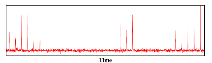
Figure 1.11.: A sequence of pulses from PSR B2319+60 observed at 1420 MHz from the Westerbork Synthesis Radio Telescope. The nulling in pulses is clearly evident.

The abrupt cessation of pulsed radio emission for several pulse periods, exhibited by many pulsars, has remained unexplained despite the discovery of this phenomenon in many radio pulsars. This phenomenon, called pulse nulling, was first discovered in four pulsars in 1970 Backer (1970c). Subsequent studies have revealed pulse nulling in about 100 pulsars to date Backer (1970c); Ritchings (1976); Biggs (1992); Vivekanand (1995); Wang et al. (2007).

The fraction of pulses with no detectable emission is known as the nulling fraction (NF) and is a measure of the degree of nulling in a pulsar. However, NF does not specify the duration of individual nulls, nor does it specify how the nulls are spaced in time. Nulling can also considered to be an extreme form of mode-changing phenomena Wang et al. (2007), in which pulsar emission goes below the detection threshold. Chapter 2 discusses the nulling phenomena in full detail.

1.6 Outline of the thesis

The aim of this thesis is to investigate the absence of pulses in pulsar, a phenomena also know as pulsar nulling. The outline of the thesis is as follows. The motivation for the work done in thesis is listed in Chapter 2. It also discusses the emission mechanism as proposed by the standard model. A summary on the previous work carried out to investigate the pulsar nulling phenomena is also included in Chapter 2. Chapter 3 discusses in details all the observations carried out for the work that has been reported in thesis. Observations from various radio telescopes are discussed and compared in the similar chapter. The common analysis techniques deployed during most of the observations are also listed in Chapter 3. In Chapter 4, details regarding the nulling behaviour of various pulsars are listed. The comparison has been made between similar NF pulsars in order to demonstrate that, the NF does not quantify nulling behaviour in full details. Chapter 4 also highlights the fact that nulling is unpredictable. Chapter 5 presents a comparison between two pulsars with high NFs. It is shown that both the pulsars exhibit similar bursting behaviour, but strikingly different quasi-periodicities and emission properties. Chapter 6 discusses the details regarding the simultaneous observations of two nulling pulsars at four different frequencies. Chapter 7 summaries the results obtained in three different studies along with their implications. The future work to extend the work carried out in the thesis is also listed in Chapter 7.

Chapter 2 Background

This chapter discusses the peculiar single pulse phenomena, exhibited by many radio pulsars, known as the pulsar nulling in full detail. The basic background regarding different relevant works that have been carried out, since the discovery of this phenomena, is also discussed with details in this chapter. In order to understand the cessation of radio emission, the chapter also highlights the standard emission mechanism model. Towards the end of the chapter, various models proposed over the years to explain the cessation of radio emission are discussed. The chapter also lists the broad motivations, for the work carried out in this thesis.

2.1 Pulsar emission mechanism

2.1.1 Neutron star

Neutron stars are born after the violent death of massive stars. When a core of a star attains the critical mass limit, after the ‘burning’ of hydrogen, the core becomes unstable to support the balance between the radiation pressure and the gravitational collapse. During this period, a chain of events occurs in which star’s core collapses in a massive explosion known as the supernova. The supernovae mainly ejects the rest of the star in a vast energy release impulsively, while collapsing the core further to form a neutron star. There are two main types of supernovae events, namely type I and type II supernovae. Type II supernovae is associated with the isolated massive stars. Type I supernovae is classified as a contact binary system of a white dwarf and a companion star, in which the companion star transfers matter to White Dwarf, there by pushing it to the Chandrasekhar limit. To distinguish between the two classes, their spectra can be studied. Type II supernovae are hydrogen rich as it was still available in the envelop surrounding the core, while type I supernovae are hydrogen depleted due to their origin from the white dwarfs. Theoretically, type II supernovae are more likely to form a neutron star because during the type I supernovae, the white dwarf is also likely to get disintegrated rather than collapse further to form a neutron star.

The neutron star avoids further collapse due to the neutron degeneracy pressure. Oppenheimer & Volkoff (1939) analysed the structure of a star consisting of degenerate neutron gas. It was shown that degeneracy was so complete that density and pressure are more important than the temperature. The relationship between the density and pressure, also known as the equation of state, have been modelled through multiple theories which can be tested by the observed relationship between the radius and the mass of the neutron star. Hence, these quantities are important to measure for a large number of pulsars. Current estimate suggest the radius of the neutron star to lie within a small range of 10.5 to 11.2 km Ghosh (2007). The theoretical limit on the neutron star masses lies between 0.5 to 2 M_⊙ Ghosh (2007). The maximum expected mass of a neutron star is about 3 M_⊙ Lattimer & Prakash (2001). Most observed values of the neutron star masses are around 1.4 M_⊙ Lorimer & Kramer (2004).

The structure of the neutron star is divided in two different regions, namely the crystalline solid crust (about 1 km thick) and liquid interior mainly consisting of superfluid neutrons. The density at the surface of the neutron star is around 10⁶ g cm^-3 which reaches to 10¹⁵ g cm^-3 near the core. The constituents of the central region could be further exotic state of matter, like mesons or kaons Baym (1991). At the exact core, neutrons are also likely to dissolve to form quarks and gluons. The surface of the neutron star is relatively less dense (about 10⁹ orders of magnitude) compared to the interior, hence its likely to be made of solid crystalline lattice, mainly of iron nuclei with a sea of free electrons flowing between them. The iron is more likely element to exist because of it’s high binding energy. The surface is believed to be extremely smooth with structure irregularity of only $\sim$5 mm because of the high gravitation potential. Neutron stars are also proposed to have very thin layer of helium Rosen & Cameron (1972) and hydrogen on the surface.

2.1.2 Magnetosphere of pulsars

Pulsars are known to be one of the highly magnetized objects in the known Universe. The magnetic field strength of pulsars ranges from 10⁸ G to 10¹⁴ G. The high energy X-ray sources, known as Magnetars, are known to have the highest magnetic field of 10¹³ to 10¹⁴ G while the old millisecond pulsars have low magnetic fields of around 10⁸ G. The direct measurements of the high magnetic fields come from the absorption lines observed in the X-ray spectra Wheaton et al. (1979); White et al. (1983). Pacini (1967) has suggested that, the magnetic flux conservation during the core compression can cause magnetic fields to reach up to 10¹² G for the neutron stars. This is possible to occur if the interior of the neutron star is highly conductive. Although, the high magnetic field has very little effect on the overall structure of the neutron star, it can alter the structure of the lattice on the surface Ruderman (1974). The primary loss of rotational energy from the neutron star is also due to the radiation caused by the high magnetic field.

The region around the neutron star were first thought to be complete vacuum due to their origin from a massive explosion which strips the envelop around the neutron star. However, in reality, it is filled with plasma of different polarities partitioned by the magnetic field, hence also known as the pulsar magnetosphere. This plasma is accumulated by pulling the charged particles from the surface of the neutron star. Deutsch (1955) was first to suggest this scenario, before the discovery of pulsars, in which rotating magnetized star would generate enough electric field to accelerate particle to substantial energies. Thus, he also suggested that accelerating particles from these magnetized star could produce cosmic rays, an idea persist to the present day. Gold (1968) suggested a model in which a bunch of particles were proposed to corotate with the pulsar, trapped in the equatorial magnetic field. However, no explanation was given regarding how such bunch would remain stable. This model was the first to propose bunching of particles which influenced future work. Ostriker & Gunn (1969) proposed a model for oblique rotator, where the magnetic and the rotation axes are not aligned, in which the loss of rotational energy was associated with the low frequency magnetic dipole radiation. The non-alignment will cause the magnetic dipole to radiate pulses. Goldreich & Julian (1969) were the first to formalize the magnetosphere around pulsars using a simple aligned rotator case. They extended the model proposed by Deutsch (1955) for the neutron stars. Although, the Goldreich & Julian (1969) model does not describe a realistic scenario, it was important work because it demonstrated, using simple electrostatics, that region surrounding the pulsar is filled with plasma of two different polarities. Multiple work for the oblique rotator have been conducted using numerical simulations to extend the Goldreich & Julian (1969) interpretation of the magnetosphere Krause-Polstorff & Michel (1985); Contopoulos et al. (1999); Spitkovsky (2004). The origin of this plasma was proposed as follows, for an aligned rotator Goldreich & Julian (1969).

The induced electric field (E_ind) at a distance (r) due to the rotation of the neutron star with magnetic field (B) would be around,

$$\bm{E_{ind}}~{}=~{}-(\bm{\varOmega}~{}\times~{}{\bf{r}})~{}\times~{}{\bf{B}}/c.$$ (2.1)

Here, $\varOmega$ is the angular velocity of the pulsar. For an aligned rotator, as assumed by Goldreich & Julian (1969), the rotation and the magnetic axes point in the $\bm{\widehat{z}}$ direction with the neutron star at the center. The angular velocity in such case can be simplified in polar coordinates as,

$$\bm{\varOmega}~{}=~{}\varOmega{cos\theta}{~{}\bm{\widehat{r}}}~{}-~{}\varOmega{sin\theta}{~{}\bm{\widehat{\theta}}}.$$ (2.2)

Similarly, the aligned dipole magnetic field at a distance r, from the center of the conducting sphere (neutron star) with radius R, can also be presented as Jackson (1975),

$${\bf B}~{}=~{}\frac{B_{p}{R^{3}}}{r^{3}}\left(cos{\theta}{~{}\bm{\widehat{r}}}~{}+~{}\frac{1}{2}{sin\theta}{~{}\bm{\widehat{\theta}}}\right).$$ (2.3)

Here, $B_{p}$ is the surface magnetic field near the pole, which can also be given as, $B_{p}~{}=~{}2\mu/R^{3}$, where, $\mu$ is the magnetic dipole moment. By putting equations 2.2 and 2.3 into equation 2.1, we can obtain the induced electric field inside the neutron star ($\bm{E_{in}}$ for $r<R$) as,

$$\bm{E_{in}}=\frac{\varOmega{B_{p}}{R^{3}}sin{\theta}}{cr^{2}}\left(\frac{1}{2}{sin\theta}{~{}\bm{\widehat{r}}}~{}-~{}cos{\theta}{~{}\bm{\widehat{\theta}}}\right).$$ (2.4)

As mentioned in Section 2.1.1, the crust region is highly conductive for the neutron stars. Thus, the charges will move and arrange inside the star to cancel the induced electric field. If outside of the sphere is taken as a vacuum in the initial conditions, the boundary conditions will allow the estimate of the electrostatics potential near the surface as,

$$\phi_{out}~{}=~{}-\frac{B_{p}\varOmega{R^{5}}}{6cr^{3}}\big{(}3cos^{2}\theta~{}-~{}1\big{)}.$$ (2.5)

The external electric field can be derived by taking a gradient of the above mentioned electric potential as,

$$\bm{E_{out}}~{}=~{}-\bm{\triangledown}\phi_{out}.$$ (2.6)

It can be shown from equations 2.3, 2.4 and 2.6 that, $\bm{E_{out}\cdotp{B}~{}\neq~{}0}$ while $\bm{E_{in}\cdotp{B}~{}=~{}0}$. Hence, the component of the electric field ($E_{\|}$) aligning the magnetic field and perpendicular to the surface at the the polar cap ($r=R$) can be given as Lorimer & Kramer (2004); Ghosh (2007),

$$E_{\|}~{}=~{}\frac{\bm{E_{out}\cdotp{B}}}{B}~{}=~{}~{}-\frac{\varOmega{B_{p}}R}{c}cos^{3}{\theta}.$$ (2.7)

The force exerted by the perpendicular induced electric field (equation 2.7) on the surface is

$$F_{\|}~{}=~{}qE_{\|}.$$ (2.8)

For a pulsar with the magnetic field of around 10¹² G, the force exerted by the induced electric field exceeds the gravitation force on the charge particles of the neutron star by many orders of magnitude (around 10⁹ for protons and more for electrons). Hence, particles get pulled out from the surface of the neutron star to cancel the electric field component (making ${\bm{E_{out}\cdotp{B}}=0}$). Moreover, the starting conditions of vacuum around the neutron star is no longer valid as it gets filled with the plasma supplied from the surface. These charge particles also experience, due to the toroidal component of the electric field (E$\perp$ to the magnetic field), $\bm{E\times{B}}$ drift, which force them to corotate rigidly with the neutron star. However, particles bounded inside the magnetosphere can only corotate to the point where their rotational velocity ($\bm{r\times{\varOmega}}$) do not cross the upper bound of the speed of light, c. This boundary is also known as the light-cylinder as mentioned in the Chapter 1 and shown Figure 2.1, reproduce here with aligned axes. The radius of the light-cylinder (R_c) is given by,

$$R_{c}~{}=~{}\frac{c}{\varOmega}.$$ (2.9)

For a pulsar with a period around 1 sec, the light-cylinder radius is around 5$\times{10^{9}}$ cm. As mentioned in Section 1.2, the light-cylinder divides the magnetic field lines in two separate regions, closed field lines and open field lines.

Figure 2.1.: Schematic diagram of a radio pulsar (not to scale) to illustrate charge density around the neutron star (in grey color) for an aligned rotator adapted by Goldreich & Julian (1969). The yellow beam is the beam of radio emission. The closed field lines are shown with green enclosed curves, while the light-cylinder is shown in background with blue color. The magnetosphere of the pulsar is divided in two parts, with negative charges on top of the polar cap and positive charges around the equatorial region. The boundary dividing the two regions occurs at $cos^{-1}(\pm 1/\sqrt{3})$ (cartoon using the free 3D modeling package : blender www.blender.org).

At any instance the magnetosphere acquires certain charge distribution, by pulling out particles from the surface, to cancel the induced electric field outside the neutron star to keep $\bm{E\cdotp{B}}=0$ (replacing $\bm{E_{out}}$ with $\bm{E}$ for simplicity). The charge distribution, required for the corotation and validity of the force free conditions (for r $\ll$ $R_{c}$), is known as the Goldreich-Julian (GJ henceforth) charge distribution and can also be expressed as Goldreich & Julian (1969),

$$\sigma_{GJ}~{}=~{}\frac{{\bm{\triangledown\cdot{E}}}}{4\pi}~{}=~{}-\frac{\bm{{\varOmega~{}}\cdotp{B}}}{2\pi{c}}.$$ (2.10)

Using equations, 2.2 and 2.3, the charge density of the particles in the magnetosphere can be estimated as,

$$n_{GJ}~{}=~{}\frac{\sigma_{GJ}}{e}~{}=~{}-~{}\frac{\varOmega{B_{s}}R^{3}}{4\pi{cer^{3}}}\left(3cos^{2}\theta~{}-~{}1\right).$$ (2.11)

The $n_{GJ}$ is known as the Goldreich-Julian charge density and it plays essential role in building the pulsar emission model. The charge density, at the polar cap for a pulsar with period of around 1 sec and magnetic field of $10^{12}$ G, is around $7~{}\times~{}10^{10}$ cm^-3. As can be seen from equation 2.11, the magnetosphere of the pulsar consist of charges with two different polarities, with a boundary at $cos^{-1}({\pm 1/\sqrt{3}})$. Figure 2.1 shows the distribution of the different polarity charge particles for an aligned rotator as assumed by Goldreich & Julian (1969) and Arons (1981). Ruderman & Sutherland (1975) assumed an anti-parallel alignment of rotation and magnetic axes, hence giving opposite polarity of charge distributions from the one shown in Figure 2.1. In both cases, the charge separated magnetosphere maintains $\bm{E\cdotp{B}}=0$ in all regions.

2.1.3 Sparking

In the open field line region, the particles are not bounded. Thus, travelling through the open field lines, they escape the magnetosphere. This creates depletion of charge particles on top of the polar cap region, causing a non-zero electric field with $\bm{E\cdotp{B}}\neq{0}$. The potential drop keeps growing on top of the polar cap as particles depart. Part of the magnetosphere, with sufficient charge particles to keep $\bm{E\cdotp{B}}=0$, pulls away from the surface of the neutron star at polar cap and a gap forms, which is the origin of the radio emission according to the standard model [Ruderman & Sutherland (1975); also referred to as RS model henceforth]. This gap is also known as the inner gap and it occurs on either poles due to quadratic nature of the electric field. The radius of the inner gap ($r_{p}$) extends from the magnetic field axis at the center to the last open field line. The RS model argues that iron nuclei (ion) has higher bounding energy and hence they can not be pulled out from the surface of the neutron star, while electrons can be pulled out easily from the surface as their binding energies are much lower. This is known as the binding energy problem. If the binding energy of the ion decreases, they can continuously flow from the surface and no such gap will grow. Consequences of such event has important implication in different pulsar nulling models (see Section 2.4.2)

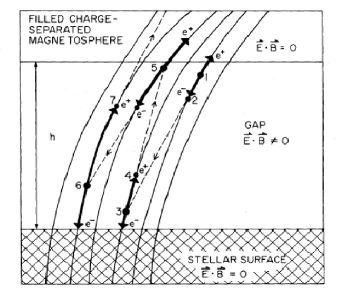
Figure 2.2.: A cross section of the polar gap. Adopted here from the Ruderman & Sutherland (1975) to demonstrate the breakdown by an avalanche of primary pair particles.

For the inner gap with height h, the potential across the gap ($\bigtriangleup{V}$) can be given in terms of the surface magnetic field $B_{s}$ and charge density $\sigma_{e}$ as Ruderman & Sutherland (1975); Ghosh (2007),

$$\bigtriangleup{V}~{}=~{}\frac{\varOmega{B_{s}}}{c}h^{2}~{}=~{}2\pi{n_{GJ}}h^{2}$$ (2.12)

As the gap between the neutron star surface and the magnetosphere ($h$) grows, the potential drop also increases ($\propto{h^{2}}$). At the instance when the gap height reaches to a limit where its equivalent to the polar cap radius ($r_{p}~{}=~{}h$), the gap attains maximum potential difference, suggested by the RS model as,

$$\bigtriangleup{V_{max}}~{}=~{}\frac{\varOmega\Phi}{2\pi{c}}~{}\sim~{}10^{12}B_{12}/P^{2}~{}~{}volts.$$ (2.13)

Here, $B_{12}$ is the surface magnetic field in units of $10^{12}$ G and $\Phi$ is the total magnetic open field line flux. However, before it acquires this limit, an avalanche of electron-positron pairs will discharge the gap potential. The discharge occurs due to the interaction of high energy background photons ($\gamma$-rays) with the high magnetic field lines on top of the polar cap. Under the influence of high magnetic field, a $\gamma$-ray photon splits into an electron-positron ($e^{-}~{}-~{}e^{+}$) pair. The gap potential then accelerates both these particles to relativistic velocities along the curved magnetic field lines in different directions. Depending upon the direction of the electric field (given model), positron or electron escapes the gap while the other falls back and hits the polar cap region. According to the RS model, positrons were speculated to escape the polar gap while the electrons travel back towards the surface (as shown in Figure 2.2). The energy of these particles, accelerate to relativistic velocities, is around $E_{e}~{}\sim~{}e(\bigtriangleup{V})~{}\sim~{}10^{11}B_{12}h_{3}^{2}/P(s)$ eV. Here, $h_{3}$ is the gap height in units of $10^{3}$ cm, while $P(s)$ is the pulsar period in seconds. The particle with this energy, moving in the curvature field lines, again emits high energy photon which in turn, again creates another electron-positron pair and so on [see Sturrock (1971); Ruderman & Sutherland (1975); Arons (1983) and Figure 2.2]. Daugherty & Harding (1986) have also suggested an alternative mechanism to produce pairs by an inverse Compton scattering the low-energy thermal photons by the accelerated charged particles. The low-energy photons may come from the surface through simple blackbody radiation due to the high neutron stars temperatures. It is not very clear which of these processes drives the pair creation but either of them create an avalanche of pairs, within $10^{4}$ cm from the surface to discharge the gap potential. This process repeats as the particles depart from the open field line region and gap again starts to grow. Sturrock (1971) was the first one to suggest the above mentioned model of pairs production through curvature radiation and continuous ejection of particle from the magnetic poles at a controlled rate in pulsars. The localized spots on the polar cap, where the magnetic field lines that caused the breakdown are anchored, are known as “sparks”. Thus, the above discussed phenomena is also known as sparking Ruderman & Sutherland (1975).

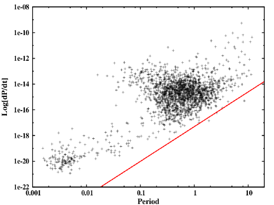
Figure 2.3.: $P-\dot{P}$ diagram of around 2000 pulsars. The red solid line is the death line, beyond which necessary conditions for pair creation does not exist. This line was derived from the relation given in Chen & Ruderman (1993). [The data were obtained from the www.atnf.csiro.au/research/pulsar/psrcat Manchester et al. (2005)]

Sturrock (1971) and Ruderman & Sutherland (1975) discussed the necessary conditions for the sparking. As pulsar gets older, it’s rotation period gets slower and slower and hence the maximum achievable polar gap potential ($V_{max}$ shown in equation 2.13) drops down. For these pulsars. the gap potential is not sufficient to create sparking and hence the necessary conditions for radio emission, discussed below, will cease. This is the death of a pulsar! Figure 2.3 shows the $P-\dot{P}$ diagram, also discussed in Chapter 1. Its clearly evident that, very few pulsars (only two or three) exist beyond the theoretically estimated death line using the standard dipole approximation Chen & Ruderman (1993). According to the standard model, pulsars are born in the upper left corner and they progress slowly to the island of normal pulsars. They eventually evolve to go beyond the death line into the what is known as the pulsar graveyard at the lower right corner in the $P-\dot{P}$ diagram.

2.1.4 Radio emission

Extensive research have been focused on developing the emission mechanism model which can give rise to observed phenomena in radio pulsars. The mechanism to generate the radio waves, with the brightness temperature of around $10^{25}~{}-~{}10^{31}~{}~{}K$, is of main interest in pulsar phenomenology. It became clear in the early days that such mechanism has to be of coherent nature, as non of the incoherent phenomena can account for such bright radiation. If there are N particles emitting coherently, the resulting emission would enhance by $N^{2}$ times the emission from a single particle during the coherent mechanism, while it only enhances by $N$ times during the incoherent mechanism. The coherent emission models can broadly be divided into three main groups of theories, viz. (a) emission by the coherent bunches [see Ruderman & Sutherland (1975); Cheng & Ruderman (1977); Benford & Buschauer (1977) and references therein], (b) maser emission, corresponding to negative absorption [see Blandford (1975); Melrose (1978, 1992) and references therein] and (c) reactive instability due to an intrinsically growing wave mode Arons & Barnard (1986); Beskin et al. (1988); Asseo et al. (1990). Each of these models have their own numerous variants, which is beyond the scope of this thesis to discuss [for a review see Michel (1991)]. Among these theories, the two-stream instability to cause bunching is the most favoured one as it has been considered by many authors Ruderman & Sutherland (1975); Benford & Buschauer (1977); Cheng & Ruderman (1977); Usov (1987); Ursov & Usov (1988); Melikidze et al. (2000); Usov (2002) and will be discussed further here. Broadly the origin of the two-stream instability can be expressed as follows.

Positrons which escape the gap on top of the polar cap, acquire relativistic velocities with Lorentz factor, $\gamma$, reaching up to $10^{6}$, which are also know as the primary particles. These high energy primary particles do not get further acceleration beyond the gap as they enter the region of the magnetosphere where $\bm{E\cdotp{B}}=0$ with $n_{GJ}$ charge density. Travelling in the curved magnetic field lines, they emit high energy photons through curvature radiation. A few of these photons again interact with the magnetic field to produce further pairs of $e^{-}~{}-~{}e^{+}$, which are known as the secondary particles. However, the energies of these secondary particles are much lower (with $\gamma$ of around $800$). In the absence of any accelerating electric field, both secondary particles pair travel in the outward direction, along the curved field line to conserve the momentum. These particles are the prime source in three different variants of two-stream instability theories which can give rise to the observed radio emission, viz. (a) interaction between primary and secondary particles Ruderman & Sutherland (1975), (b) electrostatic interaction between electron and positron of the secondary particles Cheng & Ruderman (1977), (c) interaction between clouds of secondary plasma Usov (1987); Ursov & Usov (1988); Melikidze et al. (2000).

According to the RS model, the most energetic positrons ($\gamma~{}\sim~{}10^{6}$) radiate away most of their energies within $10^{6}$cm from the stellar surface after leaving the gap. Most of these energies get converted to outward moving secondary particle pairs as discussed above. It can be shown that curvature radiation from these secondary particles falls in the radio regime Ruderman & Sutherland (1975). However, incoherent radiation from individual secondary particle can not give rise to bright radio emission seen in pulsars. To generate coherent radiation from these particle, they have to form bunches. Bunching occurs due to the Coulomb interaction between the relativistic secondary particles with the passing ultra-relativistic positrons. These positrons, generated at the later stage of the gap discharge, when the gap potential has decreased substantially, travel much further in the magnetosphere without losing much of their energies. Due to their negligible energy loss, they catch up and pass through the slow moving secondary particles cloud which causes the two-stream instability to grow and enhance the curvature radiation from bunches. Similar formalism was also suggested by Sturrock (1971). However, Benford & Buschauer (1977) have obtained more precise estimate on the development of the bunches and showed that, the beams of primary particles passing through the secondary pairs do not have enough time to develop two-stream instability. These authors have also tried to correct the RS model by invoking ion beams, originating from surface along with the positrons.

In other models of two-stream instability, Cheng & Ruderman (1977) have suggested interaction between electrons and positrons in the secondary particle pairs. It was shown by these authors that, when the secondary particles cloud moves along the curved magnetic field lines of a rotating magnetosphere, a relative streaming between electron and positron causes two-stream instability to grow and form bunches. The resultant bunch, travelling in the curved field lines, give rise to the observed radio emission. Similarly, Usov (1987) has suggested interaction between two consecutive secondary pair clouds with different momenta, which leads to two-stream instability at a distance of around $10^{8}$ cm from the surface. At these heights, the high energy particles from a lower cloud catch up with the slow moving low energy particles from a cloud going ahead of it, which causes the two-stream instability to develop. Melikidze et al. (2000) extended this model further by introducing the concept of plasma solitons, which emit curvature radiation in the radio regime.

In the above mentioned three models, the basic assumption is the non-stationary nature of the pair creation. However, Arons & Scharlemann (1979) and Arons (1981) have invoked steady pair creation, which, according to Usov (1987), may be just time average values. It is not very clear that which of the coherent emission models is operating in pulsars. Observational constraints on the emission heights has, however, confirmed the origin of emission near 50 stellar radius. At these heights, it is unlikely for the plasma instability models to be active as they are expected to occur at much higher heights. The other coherent mechanism, maser emission, requires much stronger magnetic field and thus fails to operate in millisecond pulsars which have magnetic field of around $10^{8}-10^{9}$ G. Hence, many years of extensive study has pointed out the bunching mechanism as the most viable coherent mechanism operating in rotation powered pulsars. However, it is not very clear which of the two-stream instability model is responsible for bright radio emission.

2.2 Radiation beam

The coherent radiation from pulsars, originating from one of the above mentioned emission model, give rise to conical beam of emission with the magnetic axis as a center Radhakrishnan & Cooke (1969); Komesaroff (1970). If the magnetic axis is misaligned with the rotation axis, each time this beam of emission point towards the observer, a pulse can be detected. The integrated profile, obtained from around thousand of such pulses, represents average shape of the beam for a given line-of-sight cut (see Chapter 1). This model seems to be in accord with most of the observed phenomena seen in radio pulsars.

A charge particle travelling along the magnetic field line emits curvature photon towards the observer from a point at which the line-of-sight is tangent with the corresponding field line Komesaroff (1970). Thus, the detected curvature photons also carry information regarding the orientation of the magnetic field lines at the location of their origin. This idea can be extended to speculate that, the last open field lines define the angular extent of the radiation beam and hence the width of the integrated profile also. As the open field line region is inversely related to the period of the pulsar (see equation 2.9, where $R_{c}$ is proportional to period and thus inversely related to the angular extent of the open field line region), fast spinning pulsars tend to have wider profiles, which has been confirmed by various observations.

Figure 2.4.: Emission beam geometry of a pulsar, where the rotation and magnetic axes are inclined with each other by an angle $\alpha$. The line-of-sight is shown with a red solid line which cuts the emission beam by an angle $\beta$ in the plane containing rotation and magnetic axes. The change in the longitude is measure by the angle $\phi$, which is an angle between the plane containing rotation and magnetic axes (zero longitude) with the location of the instantaneous line-of-sight, a subobserver point. The angle $\zeta$ is the angle between the subobserver point with the magnetic axis, while the angle $\Psi$ is the angle between the line joining subobserver point and magnetic axis with the line-of-sight trajectory (cartoon using the free 3D modeling package : blender www.blender.org).

The linear polarization of the observed photon, depicts the orientation of the magnetic field plane (the plane containing the field line). This linear polarization in many pulsars show peculiar variation across the pulse profiles, as discussed extensively in Section 1.4.3 by introducing the rotating-vector model proposed by Radhakrishnan & Cooke (1969). According to the model, at the origin of radio emission, the magnetic field can be assumed to be of purely dipole nature. Thus, by modelling the polarization angle changes, one can decipher the beam geometry around the line-of-sight cut. Figure 2.4 illustrates the emission beam along with the misaligned magnetic and rotation axes. The angles shown in the diagram has following relationships using simple geometry Manchester & Taylor (1977); Michel (1991).

$$tan(\Psi)=\frac{sin(\alpha)sin(\phi)}{sin(\zeta)cos(\alpha)~{}-~{}cos(\zeta)sin(\alpha)cos(\phi)}$$ (2.14)

The measured polarization angle (PA) is the angle $\Psi$ shown in Figure 2.4. Variation in the PA with $\phi$ is a measurable observed pulsar property. However, along with the different propagation effects mentioned in Section 1.4.3, there are various intrinsic phenomena which causes further changes in the polarization angle, such as the orthogonal mode changes. However, this topic is beyond the scope of this thesis to discuss further.

2.2.1 Emission height

The pulsars show gradual widening of the integrated profiles from higher to lower frequencies. This effect is known as the radius-to-frequency mapping, which suggest that, the emission regions are localized at different heights from the neutron star surface for different frequencies. Estimation of the emission heights are crucial to scrutinize different emission mechanism models, as some of them failed to operate at lower heights (as discussed in Section 2.1.4). According to Sturrock (1971) the emission region is around 1 stellar radii from the surface while Ruderman & Sutherland (1975) suggested much higher emission heights ($\approx$10-100 stellar radii). For pulsars with double profile components, separation between both of them were measured at multiple frequencies to derive the separation to frequency dependence. Komesaroff (1970) suggested this relation to be around $f^{-1/4}$ by using the curvature of the field line arguments. According to the RS model, the emission height at a given frequency is dependent upon the plasma density, given in equation 2.11, which decreases with increasing height by a factor of $r^{-3}$. Thus, these authors suggested frequency dependence of $f^{-1/3}$ for the profile evolution. Many studies have reported the emission heights in number of pulsars Cordes (1978); Rankin (1983); Lyne & Manchester (1988); Kijal & Gil (1998); Gangadhara & Gupta (2001); Mitra & Rankin (2002); Kijak & Gil (2003).

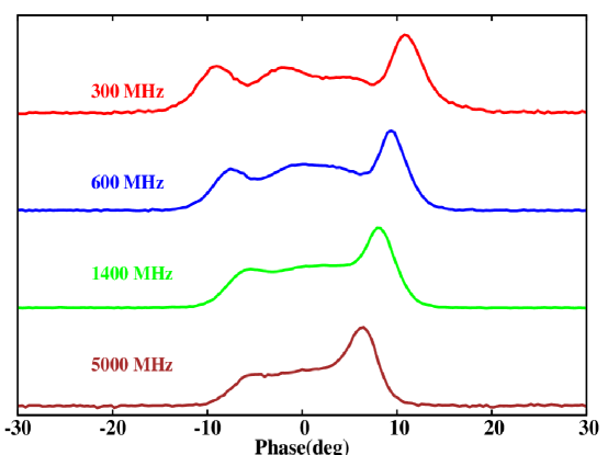
Figure 2.5.: Frequency evolution of the integrated profile for PSR B2319+60. The observations were taken at four different frequencies (viz. around 300,600,1400 and 5000 MHz) as a part of this thesis work.

Figure 2.6.: Beam of emission with localized emission regions at different frequencies for PSR B2319+60. The height and beam size were derived as explained in the text. The size and height of the emission region are in scale compare to a pulsar with radius of around 10 km. Note that these are only rough estimates and displayed here just to demonstrate the radius-to-frequency mapping (cartoon using the free 3D modeling package : blender www.blender.org).

To demonstrate the relative heights and size of the emission beams at different frequencies, we compared the integrate profiles of PSR B2319+60 at four frequencies viz. 300, 600, 1400 and 5000 MHz. The profile evolution is clearly evident in Figure 2.5 with narrow higher frequency profile to wider lower frequency profile. To estimate their relative heights, we used the relationship suggested by Kijak & Gil (2003) as,

$$r_{h}~{}=~{}400~{}\pm~{}80~{}f_{GHz}^{-0.26\pm 0.09}~{}\dot{P}_{15}^{0.07\pm 0.03}~{}P^{0.30\pm 0.05}~{}~{}km.$$ (2.15)

Here, $r_{h}$ is the emission height at frequency $f$ given in GHz, while $\dot{P}_{15}$ is the rate of change of period ($P$) in units of $10^{-15}~{}s/s$. For PSR B2319+60, Wu & Gil (1995) estimated the inclination angle $\alpha$ (31^∘) and impact angle $\beta$ (4^∘), which were used to estimate the radiation beam opening angle ($\rho$) given as Kijak & Gil (2003),

$$sin^{2}\left(\frac{\rho}{2}\right)~{}=~{}sin^{2}\left(\frac{W}{4}\right)\cdotp{sin(\alpha)}\cdotp{sin(\alpha+\beta})~{}+~{}sin^{2}\left(\frac{\beta}{2}\right).$$ (2.16)

Here, $W$ is the width of the pulse profile at the corresponding frequency. Thus, using equations 2.15 and 2.16, the beam shape at each of the observing frequency was derived and shown with a relative scale in Figure 2.6. The emission height were estimated to be around 780, 665, 535 and 385 km at 300, 600, 1400 and 5000 MHz, respectively. These heights are only rough estimates and calculated just to demonstrate the radius-to-frequency mapping of the emission regions. There are multiple effects that plays crucial role in determining these heights which are known as retardation and aberration of the emission beam due to the rotation. To estimate the true heights of emission regions, one has to correct for these effects which is beyond the scope of this thesis.

2.2.2 Rotating carousal

As mentioned in Section 2.1.3, the emission from the polar cap comes from group of localized regions (aka. sparks). The primary particle beams generated from these sparks are the sources of secondary pair plasma, which give rise to radio emission by one of the bunching mechanism. Thus, the location of sparks on the polar cap also reflects in the structure of the emission beam. Due to which, the emission beam does not have uniform illumination but, as mentioned in Section 1.5.2 and shown in Figure 2.7, constitute of small patches of emission sub-beams. These sub-beams are not stationary as they rotate around the magnetic axis due to the following mechanism.

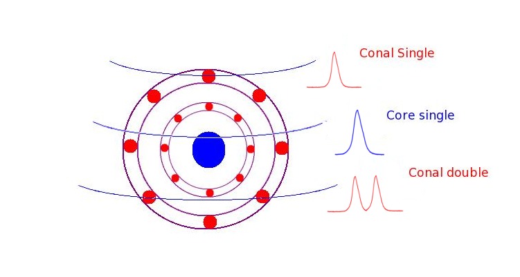
Figure 2.7.: Rotating sub-beam model to classify pulsar profiles according their line-of-sight cuts as suggested by Rankin (1983).

According to the RS model, the charge particles in the sparks do not corotate with the stellar surface (or rotate with a slightly different speed) as long as the charge densities do not reach $n_{GJ}$ (given in equation 2.11). As the gap discharges, it attains the $n_{GJ}$. At this instant, just like the particles inside the neutron star (see Section 2.1.2), the particles in the spark regions also experience $\bm{E\times{B}}$ drift. These particles move with the neutron star like a rigid rotator around the magnetic axis. Thus, the presence of the gap alters the velocity of the rotation of the spark regions. This alteration or difference in the velocity of sparks, moving around the magnetic axis, mimics a slow drifting of their locations. This difference in velocity is given by Ruderman & Sutherland (1975),

$$\bigtriangleup\nu~{}=~{}\frac{\bigtriangleup{V}}{B_{s}{r_{p}}}c.$$ (2.17)

Here, $r_{p}$ is the radius of the polar gap through which net positive charge is supplied to the magnetosphere, while $\bigtriangleup{V}$ is the potential across the gap height given in equation 2.12. As these sparks give rise to sub-beams in the emission beam, similar drifting of sub-beams can also be observed each time the line-of-sight cuts the emission cone. The periodicity of drifting is given as the time taken by a sub-beam to move to an adjacent sub-beam location. Total time taken by a sub-beam to circulate around the polar cap is around, $2\pi{r_{p}}/{\bigtriangleup{\nu}}$. If there are $n$ such sub-beams in the emission beam, the observed drifting periodicity ($P_{3}$) can be given as Ruderman & Sutherland (1975),

$$P_{3}~{}=~{}5.6~{}\frac{B_{12}}{n~{}P}~{}~{}sec.$$ (2.18)

Here, $B_{12}$ is the magnetic field in units of $10^{12}$ G, and $P$ is the pulsar period. It should be noted at this point that, along with comprehensive picture of pulsar emission mechanism, the major success of Ruderman & Sutherland (1975) was in predicting the drifting periodicity. However, van Leeuwen et al. (2003) has shown that drift velocity is not always correctly predicted by the RS model.

Komesaroff (1970) has estimated the open field line region which possess field line with sufficient curvature to produce the radio emission. Thus, intensity of the radio emission should be higher at the boundary of the open field line region, while it should vanish at the magnetic pole. Thus, he suggest a hollow cone model of the emission beam where emission is further localized in a ring of sub-beams as shown in Figure 2.7. According to which, for each line-of-sight cut, a double component profile should be observed. However, many pulsars show multi-component profiles which was explained by a introducing further concentric circular rings of sub-beams around the core component Backer (1976); Oster & Sieber (1976); Rankin (1993). Rankin (1983) classified different profiles in various categories depending upon their line-of-sight cuts (also shown in Figure 2.7), and proposed rotating carousal as the cause of drifting seen in pulsars. In later years, the carousal beam was modelled for PSR B0943+10 and number of sub-beams were calculated Deshpande & Rankin (1999, 2001). This direct modelling of the radiation beam, using single pulse observations, made the rotating carousal as one of the highly popular model.

2.3 Pulsar nulling

Among the various single pulse phenomena exhibited by the radio pulsars, absence of pulses or pulse nulling is the most peculiar one. Pulsar nulling is discussed in this section, with necessary details regarding earlier findings, as it is the core theme of this thesis.

2.3.1 Chronicles of pulsar nulling observations

Pulsar nulling was first reported by Backer (1970c) in four pulsars, PSRs B0834+06, B1133+16, B1237+15 and B1929+10. These pulsars were found suddenly to miss one to ten pulses at various times. He classified nulled pulses in two categories according to their duration and spacing. Type I nulls are the most prominent, with a spacing of about fifty pulses. Type II nulls have width of only one or two pulses and recur with spacing of three to ten pulses. Backer (1970c) claimed the nulled pulses to be periodic. To find the periodicity of these null pulses, a sequence of null and burst pulses with nulled pulses as 1 s and burst pulses as 0 s was formed. The Fourier transform of this one-zero time series was used to look for periodicity of occurrence of null pulses. He reported possible periodicity of 10.5 P, 2.8 P and 25 P (where P is the period of the pulsar) for PSRs B1929+10, B1237+25 and B1133+16, respectively. He suggested the origin of nulling due to (a) the radiation region of pulsar is undergoing some rapid changes, and (b) type II nulls are mostly related to subpulse drifting, as marching of subpulse with a spacing greater than the pulse profile could periodically cause null pulses.

In a first ever comprehensive study on the nulling pulsars, Ritchings (1976) reported nulling behaviour of 32 pulsars using the Mk IA radio telescope at Jodrell Bank. He also introduced a method to quantify occurrence of nulling using a quantity called ‘Nulling Fraction (NF)’, which quantifies the fraction of null pulses in the pulse energy sequence. His method to estimate the NF for a pulsar is discussed in Section 3.5.3. By comparing their NFs, it became possible to compare nulling between different pulsars and also to look for any possible correlations with pulsar parameters. He reported correlation of NF with the period of the pulsar and thus, concluded that the pulsars with longer period seem to posses high NFs. As the period is related to the age of the pulsar ($\propto{\sqrt{P}}$), he concluded that pulsar die with increasing fraction of nulling in them. An important characteristic reported by Ritchings (1976) is that, pulsar emission is produced in burst of pulses and the length of the burst does not depend upon the age of the pulsar. However, the separations between these bursts of pulses, also known as null states, increases with the age of the pulsar. He also suggested that, if subpulse drift is due to drifting of the spark regions in the polar cap then inactive or absence of few spark regions in the observer’s line-of-sight can sometime give rise to nulling in some pulsars. Similarly, using the Arecibo telescope, single pulse observations were conducted for 20 pulsars by Backus (1981). Out of which, nine showed nulling behaviour for which accurate estimation on the NFs were obtained.

In a further attempt to correlate nulling fraction with various pulsar parameters, Rankin (1986) reported a study of around 60 pulsars. It was claimed that nulling is quite common phenomena and should occur for half of the known pulsars. The pulsars, in the studied sample, were classified based on their integrated profile classes defined by Rankin (1983) (also shown in Figure 2.7). By comparing NFs of pulsars between different classes, she concluded that core single pulsars possess small NFs compared to other classes. Conal double and multiple component profile classes possess larger number of pulsars with high NFs compared to all other classes. In an earlier study, Ritchings (1976) concluded that pulsar die with increasing NF. Contrary to that, Rankin (1986) suggested that apparent relation of nulling and age is because of profile classes. In a given profile class, there is no strong correlation between the NF and the pulsar age. Pulsars which possess larger NFs has no greater age then those which possess small NFs in the same class. Rankin (1983) suggested that young pulsars usually have profiles with prominent core components, thus, they are likely to show small NFs Rankin (1986). She also pointed out that, nulling is a global effect as it is seen in main pulse as well as in interpulse. Thus nulling represents “global failure of the condition necessary for emission”. Weisberg et al. (1986) carried out high sensitive modulation study of around 28 pulsars, in a similar year, using the Arecibo telescope at 400 MHz. These authors concluded that, pulse energy modulation in the core component is much lower compared to conal components, thus, supporting Rankin (1986) claim of core component having smaller NFs. This study also reported NFs in around 20 pulsars for the first time.

In later years, Biggs (1992) conducted a correlation study of 72 nulling pulsars comparing their NFs with several other parameters. He observed around 25 of them at 645 and 843 MHz and compared the results with those reported in previous studies. On the basis of these observations, he concluded that in about 30% of the studied pulsars of core dominated class, nulling may be detected with higher sensitive observations. Biggs (1992) confirmed the results of Rankin (1986) about the other profile classes, with 40% of conal single, 65% of multiple profile pulsars and nearly all conal double pulsars have been observed to null. He also made similar remarks regarding the correlation of NF-age, as no correlation was seen in the same profile class. The apparent NF-age correlation is due to differences in the age between core single and conal profile classes. One of the apparent correlation which was highlighted by Biggs (1992) was about Period-NF. Pulsar with longer period seems to possess higher NF. This may indicate that pulse emission mechanism is faltering for these objects since quantities related to polar cap emission mechanisms, such as maximum potential difference across the gap, are inversely related to P (see equation 2.13). The other weak correlations which he noticed were with the rate of energy loss ($\dot{E}$) and the magnetic field at the light-cylinder ($B_{lc}$). However, these correlations can occur due to the Period-NF correlation as all of these quantities are highly correlated with the period of the pulsar. Unlike other earlier studies, Biggs (1992) reported an anti-correlation between NF and $\alpha$, thus, NF is large for small $\alpha$. Lyne & Manchester (1988) and Rankin (1990) both gave different methods to estimate $\alpha$. It was suggested by Lyne & Manchester (1988) that as a pulsar gets older, the magnetic axis tends to align to the rotation axis. Hence, the anti-correlation between NF-$\alpha$ points towards underline NF-age correlation in the Lyne & Manchester (1988) model. On the other hand, $\alpha$ estimated by Rankin (1990) does not appear to be related to pulsar age. Thus, from her model, NF-$\alpha$ correlation might have an independent origin. In any case, this correlation suggests nulling to have geometric origin. Moreover, the correlation of NF with magnetic field at light cylinder suggests that large fields are associated with the increased pulsar nulling. However this correlation is not an independent estimate, as determined value of B also depends upon $\alpha$ and period P which are, according to Biggs (1992), correlated with NF. Li & Wang (1995) also reported a statistical study of 72 nulling pulsars, contesting corrections reported by Biggs (1992). These authors concluded that, NF is more strongly correlated with the pulse width, $W$, compared to period and $\alpha$ of the pulsar. These authors also claimed that NF-$W$ correlation can also explain NF-$P$ and NF-$\alpha$ correlation reported by Biggs (1992).

The method to estimate the NF, given by Ritchings (1976), was further improved by Vivekanand (1995). With this new method, it became possible to estimate NF for the weak pulsars. Vivekanand (1995) observed around 15 pulsars and estimated NFs for 10 of them. Only two of these pulsars in the sample were new, while for the other pulsars, NFs values were improved with his new technique. He also reported similar results regarding the null and burst length as those reported by Ritchings (1976). The emission from PSR B0031$-$07 comes in burst of pulses and there are two time-scales involved. Short time-scale bursts and nulls come in $\leq$ 10 periods, while a long time-scale process can causes burst duration of $\approx$ 24 periods and null duration $\approx$ 29 periods. Vivekanand (1995) also reported that there were no truncated burst pulses before or after the null phase, indicating that subpulses are basic units of pulsar emission.

Parkes multibeam survey has discovered more than half of the known pulsars Manchester et al. (2001); Morris et al. (2002); Kramer et al. (2003); Hobbs et al. (2004); Faulkner et al. (2004); Lorimer et al. (2006). In one of such investigation, Faulkner et al. (2004) reported for the first time, nulling in a binary pulsar, PSR J1744$-$3922. Pulsars are also found in binary systems, where the other companion could be a white dwarf or a normal star [see Ghosh (2007) for a review]. The reported pulsar rotates in a tight circular orbit every 4.6 hours. The time-scale of the nulling seen in this pulsar are around few tens of minutes repeating after every few minutes of burst states. They also reported occasions where pulsar is not seen during a full 35 minute observing run. All external effects, such as scintillation and obscuring binary companion have been ruled out by these authors. The potential gap values were also calculated for non-nulling and nulling pulsars. It was suggested by these authors that nulling pulsars tend to have smaller median gap potential values and hence they are likely to null more. Similarly, PSR J1744$-$3922 was shown to have smaller gap potential which is analogues to nulling pulsars. In the similar category of strange nulling pulsars, Crawford & Lorimer (2007) reported signs of nulling behaviour in an extra Galactic pulsar, PSR B0529$-$66, located in the Large Magellanic Cloud. However, this was never confirmed.

Recently, Wang et al. (2007) carried out observations of 25 newly discovered pulsars from the above mentioned Parkes multibeam survey and estimated their NFs for the first time. Their study increased the total number of nulling pulsars by a substantial amount. Moreover, a pulsar with NF of 93% was also found, which is the largest known NF. Their study actually doubled the total number of known nulling pulsars, which possess NF above 50%. It was concluded that nulling is a property of old pulsars. It was also claimed that there is no correlation of NF and profile morphological classes as claimed by Rankin (1986). These authors showed that, almost all classes of pulsars show nulling and mulitcomponent profiles tend to have higher NFs but such pulsars are old. Thus, their study once again supported the NF-age correlation. Along with these nulling pulsars, they also reported weak mode in two of their studied pulsar. It was also claimed that nulling and mode changing are highly correlated, which was also suggested by Rankin (1986). Moreover, Weltevrede et al. (2007) reported tentative evidence of nulling in 8 pulsars but no estimates on the NFs were reported. Number of nulling pulsars were further enhanced by pulsar searches conducted from the Giant Meterwave Radio Telescope Joshi et al. (2009) and the Parkes telescope Burke-Spolaor et al. (2011, 2012).

2.3.2 Nulling$-$Drifting/Mode-changes interaction studies

Backer (1970b) reported subpulse drifting in PSR B1929+10 which was shown to have null pulses. Sub-pulse drifting is associated with nulling in many pulsars, for example PSRs B0809+74, B0818–13 and B0031–07. In the early attempts, various studies Backer (1970a); Cole (1970); Taylor & Huguenin (1971); Page (1973) have reported associated changes in the drift rate with null states. Unwin et al. (1978) have reported unique phase memory of of the subpulse location before and after the null states in PSR B0809+74. They also concluded that nulling occurs due the quenching of sparks (an intrinsic phenomena) and not caused by deflection or absorption of the radiation beam as it shows clear phase memory of subpulses across the null length. However, Filippenko et al. (1983) contested these results by showing lack of subpulse phase memory in their observations of PSR B0809+74. A more detailed account of this phenomena was reported by Lyne & Ashworth (1983) in two pulsars, PSRs B0809+74 and B0818–13. These authors showed clear changes in the drifting speed before and after the null states with estimate on the relaxation time in acquiring regular drifting behaviour directly proportional to the length of the null states. Thus, nulling in these pulsars were compared with a damped oscillator, which also has a finite relaxation time constant. Contrary to Unwin et al. (1978), these authors reported phase jumps in the subpulse location across the nulls. They suggested that these changes are due to the gradual speed up of drifting during nulls. In a similar line of investigations, Vivekanand & Joshi (1997) reported phase memory across nulls in PSR B0031–07, where a method to estimate reduction in the pulse energy during the null state was also reported for the first time. This quantity, defined as $\eta$, can put tight constrain on the possible nulling models. In the later study of the similar pulsar, PSR B0031–07, Joshi & Vivekanand (2000) reported lack of subpulse phase memory for longer null lengths. These authors also reported a change in the drift rate across nulls, exclusively noted to occur during one of the profile mode. These studies suggest that, nulling and drifting could be related in their fundamental origin or might have a similar sporadic parameter controlling them.

In a continuing attempt to study interactions between nulling and drifting phenomena, van Leeuwen et al. (2002) again looked at PSR B0809+74 with more sensitive observations. These authors classified different drift rates as two different emission modes, among which one is the normal emission mode while the later was classified as the slow drifting mode which tends to occur after all null states. They also showed increase in the intensity, with a shift in the profile towards an earlier longitude during the slow drift mode. Thus, these authors suggested that mode-changing in PSR B0809+74 is induced by nulls. In a later study, van Leeuwen et al. (2003) claimed that post nulls, the drift rates are similar to those seen at higher frequencies. Hence, during the post-null burst state, the emission originates from lower heights in the magnetosphere. Similarly, Janssen & van Leeuwen (2004) extended work of Lyne & Ashworth (1983) on PSR B0818–13 with more sensitive observations. These authors also concluded analogous behaviour, by reporting changes in the subpulse phase memory to speculate that during the nulls the drift rate appears to speed up.

Wright & Fowler (1981) reported interesting nulling behaviour in PSR B2319+60, which also shows three profile modes, also shown in Figure 1.10. These modes were classified as modes A, B and ABN in order of decreasing $P_{3}$ values (increasing drift rate) and their stability. The ABN mode showed highly irregular drifting pattern, while mode A showed very prominent stable drifting. They reported a highly correlated mode-switching and nulling. Before an onset of the null state, the modes are shown to transit from A $\rightarrow$ B $\rightarrow$ ABN, depicting an stepwise increase in the drift rate. In an interesting study of PSR B1944+17, a large nulling fraction pulsar, Deich et al. (1986) investigated similar nulling and mode-changing interactions. These authors reported four different emission modes, mode A and B with regular drift rates while mode C with zero drifting. The fourth mode, mode D, displays chaotic subpulse phase distributions. Changes between these mode were shown to triggered by the occurrence of nulls. Contrary to PSR B0809+74, this pulsar did not show any phase memory across the null lengths. The transition states, i.e. null-to-burst (and vice-versa) were shown to have different profile shapes indicating a gradual change in emission properties before the onset of the null state. A slow decrease in the intensity was also noticed which was modelled as an increasing temperature, causing gap potential to yield lower magnitudes. After a few years, in line of similar studies, Redman et al. (2005) reported interesting observations of interactions between nulling and mode changing in PSR B2303+30. The pulsar exhibited two profile modes, classified as mode B and Q. In the mode B pulsar showed regular drifting while in mode Q drifting is less ordered and it shows wider profile. Nulls were seen to occur exclusively during mode Q and also often either at the start or at the end of the mode Q. These authors also reported gradual changes in the emission from mode B to Q as damped oscillator with finite relaxation time, similar to those reported by Lyne & Ashworth (1983).

Nulling behaviour in an unusual pulsar, PSR B0826–34, with presence of emission over the entire pulse longitude, was reported by Durdin et al. (1979) at 408 MHz. It is likely that, pulsar is almost an aligned rotator with a very small $\alpha$ and a small viewing angle from the rotation axis. Moreover, the most interesting aspect of it’s emission is the high NF of around 70%, making it as one of the first known pulsar with long nulls Durdin et al. (1979). In contrast, Esamdin et al. (2005) have reported presence of weak emission during the null states, in their observations at 1374 MHz. The pulsar also showed regular drifting across 13 subpulse components. These authors suggested that, the line-of-sight always remains inside the emission beam, cutting inner and outer conal rings. They proposed a hypothesis that, nulls in this pulsar are not real and they occur due to different weak emission mode. Recently, Kloumann & Rankin (2010) reported a study on an interesting nulling and mode-changing pulsar, PSR B1944+17, which was investigated earlier by Deich et al. (1986). These authors reported analogous results regarding the presence of four drift-modes along with the 70% NF. They report a mixture of short and long nulls, in which the short nulls show weak average power. These short nulls were classified as pseudo-nulls, nulls due to the empty line-of-sights (further discussed in Section 2.3.3).

2.3.3 Periodic nulling

Excluding the first reported study of nulling phenomena by Backer (1970c), nulling was thought to be a randomly occuring phenomena and no further studies were conducted for for many decades. This view was challenged by later investigators. Navarro et al. (2003) reported periodic nulling in PSR J1819+1305. Rankin & Wright (2008) have conducted an extensive study of the same pulsar and obtained a better estimate on the nulling periodicity of around 57$\pm$1 periods. They concluded an empty line-of-sight passing between the emitting sub-beams, as the cause of periodic nulling seen in this pulsar. Rankin & Wright (2007) reported a detail study of PSR B0834+06. In the earlier studies, subpulses were considered as a basic units of emission due to the absence of truncated profiles or partial nulls Lyne & Ashworth (1983); Vivekanand (1995); van Leeuwen et al. (2002); Janssen & van Leeuwen (2004). Rankin & Wright (2007) reported such partial nulls in their study as pulses with only one of the profile component active at an instance. They reported that nulls occur after ever alternating pulses and their total observed numbers are too large for their origin from random expectation. In similar line of studies, Herfindal & Rankin (2007a) have reported a periodic feature in the pulse energy sequence of PSR B1133+16. A low frequency feature was earlier reported in this pulsar but was not confirmed with any orderly subpulse structure. Herfindal & Rankin (2007a) reported that, this low frequency feature is because of the ordered sequence of null and burst pulses. The sample of these periodic nulling pulsars were further enhanced by Herfindal & Rankin (2009). In a statistical study of the occurrence of null pulses, Redman & Rankin (2009) showed non-randomness in 14 pulsars using a randomness test known as the Wald–Wolfowitz runs test Wald & Wolfowitz (1940). These authors concluded that, this non-randomness point towards the quasi-periodic nature of the null pulses, originating from the empty line-of-sight cuts between the sub-beams. Recently, Honnappa et al. (2012) carried out observations of PSR B1133+16 at 8.35 GHz, and found supporting evidence of periodic nulling as reported by Herfindal & Rankin (2007a).

2.3.4 Broadband nulling behaviour

In a simultaneous single pulse study of two pulsars, PSRs B0329+54 and B1133+16 at 327 and 2695 MHz, Bartel & Sieber (1978) showed highly correlated pulse energy fluctuations. As nulling and pulse energy fluctuations are highly correlated, this study suggests that nulling is a broadband phenomena within this frequency range. However, later simultaneous observations of PSR B0809+74 for about 350 pulses indicated that only 6 out of 9 nulls were simultaneous at 102 and 408 MHz Davies et al. (1984). Contrary to that, Biggs (1992) reported indirect evidence of broadband nulling behaviour in many pulsars from non simultaneous observations at two frequencies viz. 645 and 843 MHz. In a first ever attempt to investigate broadband aspect of nulling behaviour, Bhat et al. (2007) reported partially simultaneous nulls in PSR B1133+16. These authors conducted simultaneous observations at four different frequencies, viz. 325, 610, 1400 and 4850 MHz from three different telescopes. They reported that, only half of the nulls occur simultaneously for PSR B1133+16. Observations at higher frequencies showed little nulling compared to observations at lower frequencies. It was concluded that, about 5% of the time pulsar showed exclusive burst emission only at the highest observing frequency, with clear nulls at lower frequencies. The profile of these exclusive pulses were shown to be extremely narrow compared to the average profile. The location of these pulses were noted to arrive at earlier phase, towards the leading edge of the pulse profile. Thus, they were suspected to have similar origin as the giant pulses. In contrast, simultaneous nulls were reported at 303 and 610 MHz for PSR B0826$-$34 Bhattacharyya et al. (2008).

2.3.5 Extreme Nullers

In the last decade, the view regarding the nulling phenomena has completely changed due to the discoveries of extreme nullers, which are sources exhibiting extreme form of nulling behaviour. These sources have been classified in two categories, first are the intermittent pulsars, which null for several days before emerging as an active normal pulsar for a few days. Kramer et al. (2006) reported a quasi-periodic nulling behaviour in PSR B1931+24, as the first of this class of known sources. B1931+24 showed complete absence of emission for around 25 to 35 days while it remained active for around 5 to 10 days. In the high cadence observations, it was observed to transit rapidly within 10 sec from an active burst state to a null state. One of the worth highlighting characteristic of this source is the changes in the $\dot{P}$. During the active state, pulsar displayed regular slow down, as expected from a normal pulsar. However, during the off-state (null), the slowdown rate decreased, suggesting an overall reduction in the energy loss. Thus, Kramer et al. (2006) suggested cessation of pair production on top of the polar cap as the cause of long off-states seen in this pulsar. In later years, three more sources were found. PSR J1841$-$0500 was observed to show off-state for around 580 days Camilo et al. (2012), while PSR J1832+0029 showed off-state for around 650 to 850 days Lorimer et al. (2012). Recently, Surnis et al. (2013) have also reported a tentative detection of intermittent behaviour in PSR J1839+15.

The second class of extreme nullers are the Rotating Radio Transients (RRATs), discovered during the reprocessing of the Parkes multibeam survey data McLaughlin et al. (2006). RRATs are pulsars which only emit single burst pulses separated by long null states lasting several seconds or minutes. They were discovered by their dispersion smear of these strong single pulses seen in their discovery plots. In the original discovery paper by McLaughlin et al. (2006), only 11 such sources were reported. However, this sample was further enhanced to around 85 sources in just 7 years of their discovery through various surveys Deneva et al. (2009); Keane et al. (2010); Burke-Spolaor & Bailes (2010); Keane et al. (2011); Burke-Spolaor et al. (2012); Shitov et al. (2009). Many of these sources are not yet published but a tentative list of them can be found at RRATalog (http://astro.phys.wvu.edu/rratalog/). Recent observations by Palliyaguru et al. (2011) reported quasi-periodicity on the time-scale of minutes to years in six RRATs. Miller et al. (2011) reported spectral behaviour of these sources, which is similar to normal pulsars. One of the strongest RRAT, PSR J1819–1458 has also been observed in optical and X-rays. The optical observations returned with negative results Dhillon et al. (2011), while the X-ray observations with Chandra and XMM Newton provided clear detection Reynolds et al. (2006); McLaughlin et al. (2007). However, the emission mechanism and the origin of their peculiar behaviour is still remain to be explained by a suitable model [see Keane & McLaughlin (2011) for a review].

2.3.6 List of nulling pulsars

In the past 44 years, since the discovery of this phenomena, around 109 pulsars were found to show nulling behaviour. These pulsars exhibit a variety in their behaviour, including interaction with drifting and mode-changing as discussed above. Table LABEL:table_all_null_psr lists most of the reported nulling pulsars in the literature, including the pulsars discussed in this thesis. NF values are listed along with their respective errors and corresponding references. It can be seen from Table LABEL:table_all_null_psr that, pulsar exhibits wide range of NFs, starting from as small as 0.0008% to as large as 93%. These pulsars also exhibit a wide range in their basic parameters, thus the operational mechanism of nulling in pulsars remain to be identified.

Table 2.1.: Table of all known nulling pulsars with their basic parameters. The columns give period, $\dot{P}$, age, surface magnetic field ($B_{surf}$), rate of energy loss ($\dot{E}$) and the reported NFs with their respective errors in the parenthesis along with the corresponding references.

No.	PSRs	P	$\dot{P}$	Age	$B_{surf}$	$\dot{E}$	NF	Ref.
		(sec)	($\times{10^{-15}}$) s $s^{-1}$	($\times{10}^{6}$) Year	($\times{10}^{12}$) G	($\times{10}^{32}$) ergs $s^{-1}$	(%)
1	B0031-07	0.94	0.408	36.6	0.628	0.192	44 (1)	This study
2	B0045+33	1.21	2.35	8.19	1.71	0.516	21 (1)	Redman & Rankin (2009)
3	B0148-06	1.46	0.443	52.4	0.815	0.0556	$\leq$ 5	Biggs (1992)
4	B0149-16	0.83	1.3	10.2	1.05	0.888	$\leq$ 2.5	Vivekanand (1995)
5	B0301+19	1.38	1.3	17	1.36	0.191	10 (5)	Rankin (1986)
6	B0329+54	0.71	2.05	5.53	1.22	2.22	$\leq$ 0.5	Ritchings (1976)
7	B0450-18	0.54	5.75	1.51	1.8	13.7	$\leq$ 0.5	Ritchings (1976)
8	B0523+11	0.35	0.0736	76.3	0.163	0.653	$\leq$ 0.06	Weisberg et al. (1986)
9	B0525+21	3.74	40.1	1.48	12.4	0.301	25 (5)	Ritchings (1976)
10	B0626+24	0.47	2	3.78	0.987	7.28	$\leq$ 0.02	Weisberg et al. (1986)
11	B0628-28	1.24	7.12	2.77	3.01	1.46	$\leq$ 0.3	Biggs (1992)
12	B0656+14	0.38	55	0.111	4.66	381	12 (4)	Weisberg et al. (1986)
13	B0736-40	0.37	1.62	3.68	0.788	12.1	$\leq$ 0.4	Biggs (1992)
14	B0740-28	0.16	16.8	0.157	1.69	1430	$\leq$ 0.2	Biggs (1992)
15	B0751+32	1.44	1.08	21.2	1.26	0.142	34 (0.5)	Weisberg et al. (1986)
16	B0809+74	1.29	0.168	122	0.472	0.0308	1.4 (0.02)	Ritchings (1976)
17	B0818-13	1.23	2.11	9.32	1.63	0.438	1.01 (0.01)	Ritchings (1976)
18	B0820+02	0.86	0.105	131	0.304	0.0638	$\leq$ 0.06	Weisberg et al. (1986)
19	B0823+26	0.53	1.71	4.92	0.964	4.52	$\leq$ 5	Ritchings (1976)
20	B0826-34	1.84	0.996	29.4	1.37	0.0622	75 (35)	Durdin et al. (1979)
21	B0833-45	0.08	125	0.0113	3.38	69200	$\leq$ 0.0008	Biggs (1992)
22	B0834+06	1.27	6.8	2.97	2.98	1.3	7.1 (0.1)	Ritchings (1976)
23	B0835-41	0.75	3.54	3.36	1.65	3.29	1.7 (1.2)	This study
24	B0919+06	0.43	13.7	0.497	2.46	67.9	$\leq$ 0.05	Weisberg et al. (1986)
25	B0940-55	0.66	22.9	0.461	3.94	30.8	$\leq$ 12.5	Biggs (1992)
26	B0940+16	1.08	0.0911	189	0.318	0.028	8 (3)	Weisberg et al. (1986)
27	B0942-13	0.57	0.0453	200	0.163	0.0963	$\leq$ 7	Vivekanand (1995)
28	B0950+08	0.25	0.23	17.5	0.244	5.6	$\leq$ 5	Ritchings (1976)
29	J1049-5833	2.20	4.41	7.91	3.15	0.163	47 (3)	Wang et al. (2007)
30	B1055-52	0.19	5.83	0.535	1.09	301	$\leq$ 11	Biggs (1992)
31	B1112+50	1.65	2.49	10.5	2.06	0.217	64 (6)	This study
32	B1133+16	1.18	3.73	5.04	2.13	0.879	15 (2)	Ritchings (1976)
33	B1237+25	1.38	0.96	22.8	1.17	0.143	6 (2.5)	Ritchings (1976)
34	B1240-64	0.38	4.5	1.37	1.34	30.3	$\leq$ 4	Biggs (1992)
35	B1322-66	0.54	5.31	1.62	1.72	13.1	9.1 (3)	Wang et al. (2007)
36	B1358-63	0.84	16.7	0.798	3.8	11	1.6 (2)	Wang et al. (2007)
37	B1426-66	0.78	2.77	4.49	1.49	2.26	$\leq$ 0.05	Biggs (1992)
38	B1451-68	0.26	0.0983	42.5	0.163	2.12	$\leq$ 3.3	Biggs (1992)
39	J1502-5653	0.53	1.83	4.64	1	4.7	93 (4)	Wang et al. (2007)
40	J1525-5417	1.01	16.2	0.991	4.09	6.17	16 (5)	Wang et al. (2007)
41	B1530+27	1.12	0.78	22.9	0.948	0.216	6 (2)	Weisberg et al. (1986)
42	B1530-53	1.36	1.43	15.2	1.41	0.219	$\leq$ 0.25	Biggs (1992)
43	B1556-44	0.25	1.02	4	0.518	23.7	$\leq$ 0.01	Biggs (1992)
44	B1604-00	0.42	0.306	21.8	0.364	1.61	$\leq$ 0.1	Biggs (1992)
45	B1612+07	1.20	2.36	8.1	1.71	0.53	$\leq$ 5	Weisberg et al. (1986)
46	J1639-4359	0.58	0.015	621	0.095	0.0292	$\leq$ 0.1	This study
47	B1641-45	0.45	20.1	0.359	3.06	84.2	$\leq$ 0.4	Biggs (1992)
48	B1642-03	0.38	1.78	3.45	0.841	12.1	$\leq$ 0.25	Ritchings (1976)
49	J1648-4458	0.62	1.85	5.38	1.09	2.93	1.4 (11)	Wang et al. (2007)
50	J1649+2533	1.01	0.559	28.8	0.763	0.211	$\leq$ 20	Redman & Rankin (2009)
51	B1658-37	2.45	11.1	3.49	5.29	0.297	19 (6)	This study
52	J1702-4428	2.12	3.3	10.2	2.68	0.136	26 (3)	Wang et al. (2007)
53	J1703-4851	1.39	5.08	4.35	2.7	0.737	1.1 (4)	Wang et al. (2007)
54	J1715-4034	2.07	3.01	10.9	2.53	0.134	$\geq$ 6	This study
55	J1725-4043	1.46	2.79	8.32	2.05	0.35	$\leq$ 70	This study
56	J1727-2739	1.29	1.1	18.6	1.21	0.201	52 (3)	Wang et al. (2007)
57	B1727-47	0.82	164	0.0804	11.8	113	$\leq$ 0.05	Biggs (1992)
58	J1738-2330	1.97	8.56	3.66	4.16	0.436	85.1 (2.3)	This study
59	B1737+13	0.80	1.45	8.77	1.09	1.11	$\leq$ 0.02	Weisberg et al. (1986)
60	J1744-3922	0.17	0.00155	1760	0.0165	0.119	$\leq$ 75	Faulkner et al. (2004)
61	B1742-30	0.36	10.7	0.546	2	84.9	$\leq$ 17.5	Biggs (1992)
62	B1749-28	0.56	8.13	1.1	2.16	18	$\leq$ 0.75	Ritchings (1976)
63	J1752+2359	0.40	0.643	10.1	0.519	3.71	$\leq$ 89	This study
64	B1809-173	1.20	19.1	1	4.85	4.3	5.8 (4)	Wang et al. (2007)
65	B1818-04	0.59	6.33	1.5	1.97	11.7	$\leq$ 0.25	Biggs (1992)
66	J1820-0509	0.33	0.932	5.73	0.567	9.59	67 (3)	Wang et al. (2007)
67	B1821+05	0.75	0.227	52.6	0.418	0.21	$\leq$ 0.4	Weisberg et al. (1986)
68	J1831-1223	2.85	5.47	8.27	4	0.0926	4 (1)	Wang et al. (2007)
69	J1833-1055	0.63	0.527	19.1	0.585	0.817	7 (2)	Wang et al. (2007)
70	B1839+09	0.38	1.09	5.54	0.652	7.76	$\leq$ 5	Weisberg et al. (1986)
71	B1842+14	0.37	1.87	3.18	0.848	14	$\leq$ 0.15	Weisberg et al. (1986)
72	J1843-0211	2.02	14.4	2.22	5.48	0.684	6 (2)	Wang et al. (2007)
73	B1848+12	1.20	11.5	1.66	3.77	2.6	$\leq$ 54	Redman & Rankin (2009)
74	B1857-26	0.61	0.205	47.4	0.358	0.352	10 (2.5)	Ritchings (1976)
75	J1901+0413	2.66	132	0.321	18.9	2.75	$\leq$ 6	This study
76	B1907+03	2.33	4.47	8.26	3.27	0.139	4 (0.2)	Weisberg et al. (1986)
77	B1911-04	0.82	4.07	3.22	1.85	2.85	$\leq$ 0.5	Ritchings (1976)
78	J1916+1023	1.61	0.681	37.7	1.06	0.0634	47 (4)	Wang et al. (2007)
79	B1917+00	1.27	7.67	2.63	3.16	1.47	$\leq$ 0.1	Rankin (1986)
80	B1919+21	1.33	1.35	15.7	1.36	0.223	$\leq$ 0.25	Ritchings (1976)
81	J1920+1040	2.21	6.48	5.42	3.83	0.235	50 (4)	Wang et al. (2007)
82	B1923+04	1.07	2.46	6.92	1.64	0.783	$\leq$ 5	Weisberg et al. (1986)
83	B1929+10	0.22	1.16	3.1	0.518	39.3	$\leq$ 1	Ritchings (1976)
84	B1931+24	0.81	8.11	1.59	2.6	5.94	$\leq$ 80	Kramer et al. (2006)
85	B1933+16	0.35	6	0.947	1.48	51.3	$\leq$ 0.06	Biggs (1992)
86	B1942+17	1.99	0.73	43.3	1.22	0.0362	$\leq$ 60	Lorimer et al. (2002)
87	B1942-00	1.04	0.535	31	0.757	0.185	21 (1)	Weisberg et al. (1986)
88	B1944+17	0.44	0.0241	290	0.104	0.111	50 (7)	Vivekanand (1995)
89	B1946+35	0.71	7.06	1.61	2.28	7.55	$\leq$ 0.75	Ritchings (1976)
90	B2016+28	0.55	0.148	59.7	0.291	0.337	$\leq$ 0.25	Ritchings (1976)
91	B2020+28	0.34	1.89	2.87	0.816	18.5	0.2 (1.6)	This study
92	B2021+51	0.52	3.06	2.74	1.29	8.16	1.4 (0.7)	This study
93	B2034+19	2.07	2.04	16.1	2.08	0.0902	44 (4)	Herfindal & Rankin (2009)
94	B2044+15	1.13	0.182	98.9	0.461	0.0488	$\leq$ 0.04	Weisberg et al. (1986)
95	B2045-16	1.96	11	2.84	4.69	0.573	10 (2.5)	Ritchings (1976)
96	B2053+36	0.22	0.369	9.51	0.289	13.4	$\leq$ 0.7	Weisberg et al. (1986)
97	B2110+27	1.20	2.62	7.27	1.8	0.595	$\leq$ 30	Redman & Rankin (2009)
98	B2111+46	1.01	0.715	22.5	0.862	0.27	21 (4)	This study
99	B2113+14	0.44	0.289	24.1	0.361	1.34	$\leq$ 1	Weisberg et al. (1986)
100	B2122+13	0.69	0.768	14.3	0.739	0.907	$\leq$ 22	Redman & Rankin (2009)
101	B2154+40	1.52	3.43	7.04	2.32	0.382	7.5 (2.5)	Ritchings (1976)
102	J2208+5500	0.93	6.99	2.12	2.58	3.39	$\leq$ 7.5	Joshi et al. (2009)
103	B2217+47	0.53	2.77	3.09	1.23	6.99	$\leq$ 2	Ritchings (1976)
104	J2253+1516	0.79	0.0665	189	0.232	0.0528	$\leq$ 49	Redman & Rankin (2009)
105	B2303+30	1.57	2.89	8.63	2.16	0.292	1 (0.5)	Rankin (1986)
106	B2310+42	0.34	0.112	49.3	0.201	1.04	$\leq$ 11	Redman & Rankin (2009)
107	B2315+21	1.44	1.05	21.9	1.24	0.137	3 (0.5)	Weisberg et al. (1986)
108	B2319+60	2.25	7.04	5.08	4.03	0.242	29 (1)	This study
109	B2327-20	1.64	4.63	5.62	2.79	0.412	12 (1)	Biggs (1992)

2.4 Why do pulsars null?

In the early studies, it was argued extensively that nulling is a property of older pulsars and they tend to lie close to the death line in the $P-\dot{P}$ diagram Taylor & Manchester (1977); Manchester & Taylor (1977); Wang & Chu (1981); Akujor & Okeke (1982); Okeke & Akujor (1982); Guseinov & Iusifov (1983); Li & Wang (1995). Hence, its worth testing this hypothesis by estimating the positions of nulling pulsars in the $P-\dot{P}$ diagram. Figure 2.8 shows the distribution of all nulling pulsars (listed in Table LABEL:table_all_null_psr). Its clearly evident from this distribution, in the $P-\dot{P}$ diagram, that they are not localized near the death line. Moreover, it should be noted, that pulsars with high NFs lie right in the middle of the normal pulsar population. Thus, its unlikely that nulling presents dying state of a radio pulsar. Similar conclusions were also suggested by Michel (1991).

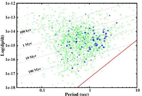
Figure 2.8.: Nulling pulsars in the $P-\dot{P}$ diagram with the population of normal pulsars zoomed in. The nulling pulsars are shown with a blue points while their shape represented their corresponding NFs range. These NFs were binned in five groups, to show their relative localization, which are (1) NF$\leq$5% with pluses, (2) 5%$<$NF$\leq$15% with crosses, (3) 15%$<$NF$\leq$30% with triangles, (4) 30%$<$NF$\leq$60% with squares and (5) NF$>$60% with pentagons. The green points are the normal pulsars while the red solid line is the speculated death line according to the model given by Cheng & Ruderman (1977). The characteristic age of the pulsar are also shown with the dashed lines.

If nulling is not due to the age of the pulsar, then certain mechanism, operating along with the emission processes, may cause faltering of the radiation beam. There are two different group of theories in literature that attempt to explain the cause of nulling. First group of theories are more inclined towards changes in the geometry of the beam and the line-of-sight, while the second group of theories suggest intrinsic effects that can cause cessation of the full radiation beam.

2.4.1 Geometric effects

In the line of geometric reasoning, Arons (1983) proposed nutation of the emission beam as a likely cause. In Section 2.3.3 missing line-of-sight as one of the geometric effects was briefly discussed. This model was proposed due to the observed periodic fluctuations seen in a few nulling pulsars. According to which, the line-of-sight cuts between the radiating sub-beams, and thus missing the emitting regions. It is also possible that, only a few radiating sub-beams extinguished and when line-of-sight passes over them, nulls are observed. As the sub-beams are organised in an evenly spaced uniform pattern (Figure 2.7), empty line-of-sight cuts or extinguished individual sub-beams are more likely to repeat after certain pulsar periods. Ritchings (1976) concluded, for the first time, the geometric origin of nulling phenomena due to these extinguishing sub-beams in his study. This was attributed as the nulling periodicity Herfindal & Rankin (2007a, 2009); Rankin & Wright (2008).

In further models of geometric origin, Dyks et al. (2005) suggested reversal of emission beam for PSR B1822$-$09 to explain the peculiar main pulse and interpulse relation. This pulsar exhibit strong main pulse with a precursor. Precursors are known as the pulse component in front of the main pulse, separated by a few degrees in longitude [see Gil et al. (1994) for a review]. PSR B1822$-$09 exhibit interesting anti-correlation between this precursor and interpulse, as when the precursor goes in the null state the interpulse emission appears and vice-verse Gil et al. (1994). Thus, Dyks et al. (2005) suggested that, the interpulse and the precursor are likely to originate from the same side of the emission beam. The emission seen during the interpulse is simply reversed emission coming from the precursor, from the main emission beam facing away from the observer. Thus, during these occasions, emission in the precursor beam reverses it’s propagation direction. If such action takes place in the main beam also then it will give rise to the observed null pulses. However, recent studies from Backus et al. (2010) showed that during many pulses, the precursor and the interpulse are both present in PSR B1822–09. Thus, its unlikely that such emission reversal exist for this pulsar.

In other models, Zhu & Xu (2006) reported precession of the rotation axis as the cause of nulling to explain absence of regular emission from one of the transient sources near the Galactic centre namely, GCRT J1745–3009. However, the precession in pulsars are very rare as there are only a few tentative evidence Weisberg et al. (1989); Cadez et al. (1997); Jones & Anderson (2001); Heyl & Hernquist (2002); Weisberg & Taylor (2005). Moreover, Glendenning (1990) reported deformation of the emission beam due to the misalignment between the rotation and the neutron star symmetry axes. However, it should also be noted that, such models are likely to give periodic oscillations in the pulse energy with consecutively occurring null and burst states. In other studies, Clemens & Rosen (2004) reported non-radial oscillation as the cause of may single pulse phenomena including nulling, drifting and mode-changing. These authors suggest that mode-changing and nulling are due to the changes between different oscillation modes.

2.4.2 Intrinsic effects

In the RS model, as explained in Section 2.1.4, the coherent radiation is a highly tuned process. Change in any of the necessary conditions of coherence may lead to stoppage of emission. In the early years, Cheng (1981) suggested fluctuations in the temperature to invoke changes in the coherence conditions as a possible cause of nulling. Deich et al. (1986) also reported possible increase in the temperature, which can cause ion outflow and extra X-ray flux, to decrease the polar cap potential to stop sparking and primary particle flow. This rise in temperature can occur due to the backflowing electrons, generated during the sparking action, hitting the polar cap region with relativistic velocities. The heated up spark regions (also known as the hot spots) are more likely to produce further pairs on top of them in the consecutive sparking action (post null). Thus, this model was proposed as the reason for the reported subpulse phase memory across the nulls in B0809+74. Deich et al. (1986) also estimated the null-to-burst (and vice-versa) transition time-scales of around 2 to 30 milliseconds, which is equivalent to the subpulse widths. Thus, it was also suggested as an explanation for the lack of partial nulls in B0809+74. However, these claims were contested by Filippenko & Radhakrishnan (1982) and later observations from Filippenko et al. (1983). Filippenko & Radhakrishnan (1982) showed that, these hot spots will cool too fast to persist any memory on the time-scale of null lengths. In contrast, they proposed a model of continuous flow of charge particle as the cause of nulling. In their model, the polar gap potential attains a stationary state in which gap discharges roughly at the same rate as it charges, thus the flow of primary particle does not stop. However, in an non-stationary flow, as discussed in Section 2.1.4, any of the proposed two stream instability conditions will not be satisfied to produce bunching. Thus, this stationary flow of primary plasma may give rise to absence of emission. This polar cap potential can suddenly discharge also, retaining normal interrupted sparking to cause non-stationary flow to form bunches again. To explain the memory across nulls, Filippenko & Radhakrishnan (1982) invoked the mechanism of flux tubes through which the particles are transferred to the magnetosphere to form sub-beams. The electric field in these flux tubes are much higher compare to regions between them, and thus they are more likely to produce sparking. During the post-null state also, the sparking takes place inside these tubes to retain the subpulse phase memory.

Kazbegi et al. (1996) reported a model of nulling in pulsars considering a different emission mechanism proposed by Kazbegi et al. (1991). According to Kazbegi et al. (1996), the drifting of subpulses are not due to the shifting spark regions, but rotation of plasma wave around the magnetosphere. Particles are extracted from the surface to form a primary beam distribution. The most energetic particles of this beam give rise to secondary plasma and backflowing particles. These backflowing particles heat up the surface, which causes broadening of the primary beam energy distribution. As this process repeats several times, gap potential slowly drops (on much larger time-scale compared to RS sparking). Thus, the distribution of the primary plasma moves towards the low Lorentz-factors, ultimately switching off the emission mechanism. When the gap attains the $n_{GJ}$, it closes to charge again as pulsar retains its emission state. This phenomena is different from the RS model, in which gap discharges roughly on the time-scale of a few microseconds. However, in the Kazbegi et al. (1996) model, the gap discharges on the time-scale of primary beam distribution function. Thus, if this process takes more time than the pulsar period, nulls can be observed. One of the main argument that can be put forward to contradict this model is the speculated emission height. This theory suggest generation of radio emission around 10 to 20% height of the light cylinder, which is around 5000 times stellar radii. However, recent observations have confirmed the hight of emission to be around 50 stellar radii Cordes (1978); Rankin (1983); Lyne & Manchester (1988); Kijal & Gil (1998); Gangadhara & Gupta (2001); Mitra & Rankin (2002); Kijak & Gil (2003).

As discussed in Section 2.1.3, the gap discharge can occur due to (a) avalanche of pair plasma triggered by the photons created from the curvature radiation (CR) or (b) by inverse Compton scattering (ICS) of the thermal photons from the relativistic charged particles ejected from the surface. In the original RS model, the ICS process was assumed to be very inefficient mechanism and hence was not considered. However, Daugherty & Harding (1986) suggested that due to the strong magnetic field, ICS could be an efficient mechanism. Zhang & Qiao (1996) argued that in case of ICS gap discharge, the surface temperature plays an important role. If the temperature is above certain threshold, the binding energy of ions will decrease, which can cause the ion flow from the surface to extinguish the polar gap (as suggested in Section 2.1.3), and ultimately to cause nulls. Zhang et al. (1997) proposed that a mixture of CR and ICS discharge might be operating with different temperature ranges in a same pulsar to explain the observed mode-changing phenomena. Zhang et al. (1997) extrapolated this model to nulling pulsars, specially for PSR B1055–52. They argued that normally the gap remains in a thermal ICS mode, which causes relatively low gap height but very energetic secondary particles. In contrast, the resonant ICS mode has higher gap height and low energy secondary plasma. When pulsar switches from thermal ICS to resonant ICS mode, due to the temperature fluctuations, the secondary pair plasma will not have sufficient energy in this pulsar to maintain the coherence conditions, and it exhibits nulls.

The chemical composition and structure of the neutron star also plays an important role in characterising its emission behaviour. Section 2.1.1 discusses the constituents of the surface materials and also highlights that the surface of the neutron star is smooth. However, Vivekanand & Radhakrishnan (1980) showed that, it is possible for the neutron star surface to have irregularities of the order of around 10 cm. These tiny hills on the polar cap region will have different electric potential on top of them. Thus, they can heavily affect the outflow of particles. Vivekanand & Radhakrishnan (1980) showed that this 10 cm hill can cause 10³ times fluctuations in the pulse energy, which was proposed as a possible cause of brighter and weaker profile modes seen in a few pulsars. This model can be extrapolated to suggest that it can also cause the radio emission to go below the detection threshold of the telescope to produce nulls.

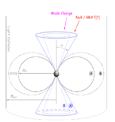
Figure 2.9.: Schematic view of the pulsar magnetosphere adapted here from Timokhin (2010). The two magnetospheric states are indicated with A and B to highlight the differences in their opening angles. Switching between these states can cause pulsar to display mode-changes or nulls depending upon the viewing angle.

In the recent study, Timokhin (2010) reported interesting model for nulling and mode-changing pulsars. The motivation for his proposed model was to explain the $\dot{P}$ variations seen in the intermittent pulsars as they suggest an underline phenomena on a global magnetospheric scale during the nulls. Timokhin (2010) proposed two different scenarios which can keep the entire magnetosphere in different configurations. These include (1) configurations with different close field line regions as shown by Timokhin (2006) and (2) configurations with different current density distributions Contopoulos (2005). The magnetosphere of a pulsar can switch between different close field line regions or it can switch between different current density distributions or both. However, the emission beaming angle will change for any type of above mentioned state changes, to cause nulling as shown in Figure 2.9. For an outer line-of-sight cut pulsars, the change in the beaming angle can cause the entire emission to propagate away from the observer and thus nulls will be observed. For the pulsars with slightly inner cut, such changes will allow sampling of different parts of the emission region to show different sub-beam structures with different integrated profiles. Timokhin (2010) argued that the difference between the rate of energy loss for both types of state changes is similar to explain the $\dot{P}$ changes during the nulls in the intermittent pulsars.

2.4.3 External effects

There are also models proposed in various studies which are related to magnetospheric changes triggered by external influences. Michel (1991) suggested that nulling might be due to accretion of interstellar medium to pulsar magnetosphere. In a more recent study, Cordes & Shannon (2008) reported influence of asteroid belt around the pulsars to cause various temporal changes. This “cirumpulsar” debris entering the light cylinder can change the conditions for pair productions and coherence, which can cause cessation of observed emission. Cordes & Shannon (2008) argued that the time-scale of this phenomena ranges from seconds to months to trigger nulling as well as intermittency of radio emission.

2.5 Motivations for this study

Pulsar nulling remained an unexplained phenomena even after many decades of investigations. The fundamental question, Why only a few pulsars null and others do not?, remain unanswered. Various models have been proposed which aim to tackle the problem for individual cases. However, a broad overall picture regarding the true nature of the nulling phenomena has escaped a satisfactory explanation. The reason could be a lack common agreement between different studies regarding the correlations of NFs with different pulsar parameters. For example, Ritchings (1976) reported NFs are correlated with the age of the pulsar while Rankin (1986) contradicted these claims by showing correlations with profile classes. These claims were also contested by later studies conducted by Wang et al. (2007) to show that all profile classes of pulsars show similar nulling behaviour. Moreover, the degree and form of pulse nulling varies from one pulsar to another even though they exhibit similar NFs. On one hand, there are high NF pulsars such as PSR B1931+24 which shows absence of emission for several days Kramer et al. (2006), while there are pulsars such as PSR J1752+2359 Lewandowski et al. (2004), which exhibits nulls for only for 3 to 4 minutes, while exhibiting similar NF. Thus, it is possible for two pulsars to have similar NF while their nulling time-scales could be complete different, which raises an important question, does the NF of a pulsar an ideal way to quantify it’s behaviour?

Similarly the broadband aspect of the nulling behaviour remains ambiguous due to various contradictory studies. For example, a few studies have shown the nulling to be a broadband phenomena Bartel & Sieber (1978); Bhattacharyya et al. (2008), while a a few other studies have contested these results by showing lack of concurrent behaviour Davies et al. (1984); Bhat et al. (2007). In light of all these previous investigations, long, sensitive, and preferably simultaneous observations at multiple frequencies of a carefully selected sample of pulsars are motivated. The main motivations behind the major part of the work carried out in this thesis can be listed as follows.

1. The nulling behaviour of similar NF pulsars should be compared to quantify their differences.

2. Nulling behaviour should be quantified incorporating their time-scales.

3. The periodicities observed in the nulling phenomena by recent observations are intriguing to scrutinize for a large number of pulsars.

4. Broadband aspect of the nulling phenomena needs to be investigated from more number of pulsars with sensitive and simultaneous observations at wide range of frequencies.

Thus, the aim of this thesis is to quantify, model and compare nulling behaviour between different classes of pulsars to scrutinize the true nature of the nulling phenomenon at multiple frequencies.

Chapter 3 Observations and Analysis

3.1 Introduction

This chapter focuses on the details of the observations and the data analysis procedures carried out in this thesis. The first part discusses the details regarding the observations carried out using the Giant Meterwave Radio Telescope (GMRT), the Westerbork Synthesis Radio Telescope (WSRT), the Effelsberg and the Arecibo radio telescopes. In the second part, analysis procedures followed for the data reductions have been discussed briefly. Table 3.1 lists all the pulsars that were observed as a part of this thesis work along with the observing frequencies and the approximate number of observed pulses for these pulsars. For two pulsars (PSRs B0809+74 and B2319+60), observations were carried out simultaneously at four different frequencies, which includes the GMRT at 313 and 607 MHz, the WSRT at 1380 MHz and the Effelsberg at 4850 MHz. For PSR J1752+2359, long observations were carried out from the GMRT. Along with that, archival data from shorter independent observation from the Arecibo telescope were also investigated. The prime motivation behind these observations are listed in Section 2.5. Moreover, a few observations were also conducted on the newly discovered pulsars to enhance the number of known nulling pulsars (motivation for these observations are mentioned in Sections 3.3 and 4.1).

JName	BName	Period	DM	Flux at	Frequency of	N
				1400 MHz	observations
		(sec)	(pc cm-3)	(mJy)	(MHz)	(Pulses)
J0814+7429	B0809+74	1.292241	$6.1$	$10.0$	325, 610,	13000
					1380, 4850
J0820$-$1350	B0818$-$13	1.238130	$40.9$	$7.0$	610	3400
J0837$-$4135	B0835$-$41	0.751624	$147.2$	$16.0$	610	3400
J1115+5030	B1112+50	1.656439	$9.2$	$3.0$	325	2700
J1639$-$4359†	$-$	0.587559	$258.9$	$0.92$	610	13000
J1701$-$3726†	$-$	2.454609	$303.4$	$2.9$	610	2500
J1715$-$4034†	$-$	2.072153	$254.0$	$1.60$	610	1600
J1725$-$4043†	$-$	1.465071	$203.0$	$0.34$	610	2500
J1738$-$2330†	$-$	1.978847	$99.3$	$0.48$	325, 610	8000
J1752+2359	$-$	0.409051	$36.0$	$3.50$	610	52000
J1901+0413†	$-$	2.663080	$352.0$	$1.10$	610	2600
J2022+2854	B2020+28	0.343402	$24.6$	$38.0$	610	8000
J2022+5154	B2021+51	0.529196	$22.6$	$27.0$	610	1400
J2037+1942	B2034+19	2.074377	$36.0$	$-$	610	1600
J2113+4644	B2111+46	1.014685	$141.3$	$19.0$	325,610,	6200
					1380,4850
J2321+6024	B2319+60	2.256488	$94.6$	$12.0$	325, 610,	10000
					1380, 4850

Table 3.1.: Observed list of pulsars with their basic parameters. The columns give, Pulsar name, Period of the pulsar, Dispersion measure, Flux of the pulsar reported at 1400 MHz, Frequencies of observations, and number of observed pulses. Pulsars marked with a dagger are the newly discovered pulsars from the Parkes multibeam pulsar survey.

3.2 Selection of observing frequencies

Observations of the recently discovered pulsars, reported in this thesis work, were carried out at 610 MHz with the GMRT. However, observations of many known nulling pulsars were carried out at various other frequencies, as listed in Table 3.1. The GMRT is capable of operating at six different frequencies. The choice of the observing frequency depends upon many factors. However, the most important factor that drives the selection of observing frequency is the source’s flux density at that particular frequency. Pulsars are intrinsically stronger at lower frequencies. Dependence of the pulsar flux density with the observing frequency can be expressed as,

$$S_{\nu}~{}\propto~{}\nu^{-\alpha}.$$ (3.1)

Here, $\alpha$ is the spectral index and S_ν is the flux density at an observing frequency $\nu$. Most of the pulsars exhibit negative spectral indices, which makes them stronger in flux as one goes to lower and lower radio observing frequencies.

Only a few pulsars were observed at 325 MHz while rest of the newly discovered pulsars were observed at 610 MHz. At frequencies around 325 MHz, the Galactic noise, due to the emission from the interaction of the charge particles with the Galactic magnetic fields, will dominate the background noise. It would also become much more difficult to phase equalise the antennas with larger baselines for longer duration at lower frequencies (see Section 3.4.1.1). Many of the newly discovered pulsars have high DM and situated near to the Galactic centre. These pulsars suffer large scattering, which reduces their single pulse sensitivity at 325 MHz (as discussed in Section 1.3.2 and shown in Figure 1.4). Hence, relatively lower frequency of 610 MHz was used for most the observations of the newly discovered pulsars to overcome these effects as well as to take advantage of the negative spectral indices.

3.3 Study of newly discovered pulsars

The GMRT was used to study some of the recently discovered nulling pulsars in this thesis work as it has an advantage of larger collecting area along with a wider low frequency coverage. In the last few years, several new pulsars have been discovered. For example, the Parkes Multibeam Survey (PKSMB) has discovered around 800 pulsars in the last decade Manchester et al. (2001); Morris et al. (2002); Kramer et al. (2003); Hobbs et al. (2004); Faulkner et al. (2004); Lorimer et al. (2006). Analysis on the PKSMB data with improved techniques still promises to enhance this number. As mentioned in Section 2.3.5, RRATs are one of such example, which were discovered in the reprocessing of the PKSMB data McLaughlin et al. (2006). Among all of these recently discovered pulsars, several of them show interesting single pulse intensity variations. However, many of these have not been systematically studied to investigate pulsar nulling. Thus, to investigate this further, discovery plots of around 600 pulsars were studied carefully in order to find indication of nulling in them. Out of this sample, 93 seem to exhibit nulling like behaviour.

The GMRT can only observe pulsars which are located higher than $-50^{\circ}$ in the declination. As all these pulsars were discovered by the Parkes telescope, some of them are located deep in the southern sky. Out of 93 selected candidates, 13 are located outside the GMRT observable sky range. The remaining 80 pulsars were categorised according to the pulse intensity variations seen in the discovery plots. In some of these pulsars, degree of pulse intensity variations clearly suggest nulling. In other cases, it is difficult to make clear judgement about the possible nulling because of low S/N. Third criteria for selection of suitable observable candidates, is based on the choice of an appropriate observing frequency.

To estimate, whether a particular pulsar is above the sensitivity limit of the GMRT, it is essential to know its flux densities at 325 and 610 MHz. Most of the known pulsars exhibit spectral index of around -1.8$\pm$0.2 Maron et al. (2000). PKSMB pulsars were discovered at 1420 MHz so for most of our candidates, flux densities were reported only at 1420 MHz. A few of these pulsars, among the selected candidates, have reported flux densities at 400 MHz. For these pulsars, the known spectral indices were used to calculate the flux densities at 325 and 610 MHz. While for the remaining pulsars, flux densities at 325 and 610 MHz were calculated using their 1420 MHz flux density with an assumed common spectral index of $-$1.8. Only those pulsars were selected for the final observations, which showed reasonably high expected single pulse sensitivity (i.e. expected S/N $>$ 5).

3.4 Radio Telescopes and Observations

3.4.1 The GMRT

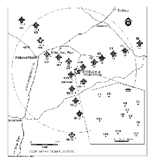
Figure 3.1.: The GMRT array of 30 dish antennas, located at +74^∘03$\textquoteright$E and +19^∘06$\textquoteright$N at Khodad, India (Courtesy : Prem Kumar)

The observations with the GMRT were carried out during the cycle 15, 16, 18 and 19 under the project name of 15VRG01, 16$\_$048, 18$\_$036, 18$\_$071 and 19$\_$022 between 2008 to 2011.

The individual dishes of the GMRT are 45-meter in diameter. Their reflecting surface forms a paraboloid which allows the parallel waves to converge to one common point. If the parallel waves fall on the dish, then the reflected waves will still remain in phase at the focal point of the dish which is also known as the feed. There are five dipole/cylindrical feeds, corresponding to the central frequencies of 150, 233, 327, 610 and 1420 MHz, mounted on the four faces of a rotating turret at the focal point. The feed detects both the approaching polarisation components from the sky. The antenna has two axes of rotation to point towards any direction in the sky through its azimuth and elevation electric motors. The elevation axis has a limit of 17.5^∘ from the horizon. The reflecting surface of the dish is a rectangular mesh which allows the antenna to operate in comparatively higher wind speeds. It also reduces the load on the electric motors which cuts down the construction cost by a large margin. Due to this design of the reflecting surface, the maximum operating frequency with this dish is around 3 GHz. The size of the mesh is also not uniform. The inner one third of the dish has a mesh with the size of 10 mm $\times$ 10 mm, the middle one third has the size of 15 mm $\times$ 15 mm and the outer one third has the size of 20 mm $\times$ 20 mm. The available effective area at 1420 MHz is smaller related to the other frequencies due to a comparatively bigger size of the mesh in the outer area, which does not act as an efficient reflecting surface at 1420 MHz.

The inner part of the array is called a central square (CQ). The CQ is 1 km$\times$1 km in size and contains 14 antennas. The purpose of these antennas is to provide short baselines specially for wide field imaging and pulsar observations Swarup et al. (1991). Rest of the 16 antennas are distributed in a $\textquoteleft$Y$\textquoteright$ shaped configuration as shown in Figure 3.1. The three arms according to their positions from the CQ are called the eastern, the western and the southern arms. The eastern and the southern arms contain five antennas each while the western arm contains six antennas. The longest baseline possible with the GMRT is 25 km long. The antennas in the arms make the GMRT a very important instrument for high resolution imaging by an unique technique called the earth rotation aperture synthesis. However, this will not be discussed in this thesis as non of the observations used the imaging capabilities of the instrument. To study the single pulse behaviour of the nulling pulsars, we used the GMRT in a single dish mode which will be discussed in the following sections. The GMRT provided very valuable and high sensitivity observations to investigate single pulse behaviour with its large collecting area and good frequency coverage.

3.4.1.1 Selection of antennas

The GMRT was used in a phased array mode for all the observations reported in this thesis. To construct a phase array beam, the instrumental phase differences between the array antennas need to be compensated. This procedure, called the phasing, uses a strong point source to estimate phases of the array antennas with respect to a reference antenna. The instantaneous phase of the astronomical signal received by a given antenna depends on the signal’s path through the ionosphere which can exhibit turbulence due to various external factors. Thus, antennas which are widely separated (i.e. antenna pair with a long baseline), receive signals from completely different ionospheric zones above them. At lower frequencies, the ionospheric changes are comparatively rapid for long baselines, hence it is not possible to phase equalise such antennas for more than two hours. The observations at 325 and 610 MHz were carried out with only short baseline antennas (CQ + 6 antennas) to keep the respective phase fluctuations minimum during a single stretch of two hours long observations. Prior to any schedule observations, all fourteen CQ and first two antennas of each arm were selected (i.e. total 20 antennas). However, during the observations, only 16 to 17 of these antennas could be used due to the following reasons concerning their performance.

To conduct the observations at a particular frequency, the feed for the required frequency was rotated and pointed towards the dish. For all the selected antennas, a solar attenuator, situated inside the feed, was set to 14 dB in order to get rid of the excess Galactic background at 325 MHz. Before the observations of the targeted source, the pointing offset experiment was carried out to estimate the sensitive and the beam pattern for each antenna. During the pointing offset experiment, a strong point source was selected (either Cassiopeia A or Cygnus A). All selected antenna beams were scanned across the source in order to get the beam pattern. The beam pattern of each antenna was carefully examined to identify any anomaly. The corresponding offset in the pointing for individual antenna was corrected manually. For any known strong point source, there are corresponding counts an antenna should provide as an output from the calibrated back-end. Hence, the sensitivity of the antenna can be determined from the corresponding counts it displayed on the observed strong point source. Those antennas which showed degraded sensitivity were excluded before the observations. At the start of the observations, it is essential to equalise the default output power from all the antennas. Those antennas which even after a manual adjustment failed to reach the required power level were also excluded before the observations. After carrying out power equalisation, all selected antennas were also phase equalised to give minimum phase difference with a reference antenna. Only those antennas were selected which showed phase differences within acceptable limits ($\pm$ 20^∘) across the entire frequency band. Phasing is however not possible for a few of the selected antennas, as occasionally the true instrumental power is masked by the radio frequency interference (RFI). Those antennas, for which phasing was not successful, were not included. Band shapes of all the antennas were also observed carefully in order to find any significant RFI lines in any frequency channel. Those antennas which showed RFI were excluded from the observations. Every exclusion of an antenna from the array will degrade the sensitivity of the experiment, hence it is not possible to throw away more than 3 to 4 antennas. In the final selection, one has to find a balance between the degradation of the sensitivity and the antenna quality.

For initial studies of the newly discovered pulsars and the a few of the known nulling pulsars, hardware backend was used (Cycle 15 and 16). For rest of the observations, a newly developed software backend was used. First the settings for the hardware backend are described and later the settings for the software backend will be discussed. The I^st local oscillator (LO) needs to be set such that the corresponding RF gets converted to an intermediate frequency (IF) of 70 MHz with 32 MHz bandwidth. For the observations at 325/610 MHz as an observing frequency, I^st LO was set at 255/595 MHz respectively. These signals were again modulated to the optical wavelengths to transfer them through the optical fiber links to the central electronics building. The same procedure was applied to both the polarisation outputs.

3.4.1.2 Hardware backend and settings

In the central electronics building, the optical wavelengths were down-converted to obtain the 70 MHz IF for each polarisation. The retrieved signal were again down-converted to baseband using a IV^th LO of 70 MHz in the baseband system. This conversion was carried out using a quadrature mixer splitting the overall 32 MHz band in two 16 MHz sidebands, namely the Upper side band (USB) and the Lower side band (LSB). The baseband also has an Automatic level control (ALC), which is usually switched off during the pulsar observations for the following reasons. The purpose of the ALC is to keep the signal in an optimum range (i.e above quantization error limit but below saturation limit). The ALC flattens the changes in the signal passing through it. The pulsar signals on the other hand are train of pulses. The ALC introduces a distortion to the pulsar signals because of the inherent finite time constant. Hence, it is essential to keep the ALC off during the pulsar observations. The signals were then orderly processed by the analog-to-digital converter (ADC), the delay processing units and the FFT engines. The FFT unit was configures to take 512 points FFT, which corresponds to 256 channels across the observed bandwidth. The output of the FFT is a time multiplexed polarisation data with 256 channels in a time-series. The output was then transferred to the corresponding USB or the LSB GMRT Array Combiner (GAC) unit.

GAC first demultiplexes both the polarisation channels. The phased array output is produced by taking a sum of the voltages from each antenna and then adding them for the final detection Prabhu (1997). An additional selection of gain values were made inside the GAC. One has to choose the gain values with a certain precision, between 1 to 15 with a 3 dB step, because the lower gain value will introduce the quantization errors and the higher gain value will saturate the output signals. For these observations, gain value number 8 was selected. The GAC permits the users to select their choice of antenna to be added in the phased array beam. After considering various issues related to individual antennas (as discussed in section 3.4.1.1) final selections were made in the GAC output. Same antennas were selected for both the USB and the LSB.

The GAC-USB is connected to the Phased Array (PA) backend while the GAC-LSB is connected to the Polarimeter pulsar backend (PMTR). Both the backends were configured to give an integration time of around 1 msec. The output from these backeds are also time multiplexed polarisation data similar to output of the FFT units. These backends can be configured to provide the Stoke’s parameters or the cross and the self power terms. However for these observations, only total intensity modes were used for both the USB and the LSB. In this configuration, both the polarisations were combined together in the backends and the total intensity outputs were produced. The pulsar backends also provide intermediate GPS bits, which can be used to get a time stamp for the recorded data. The general information regarding the start and the stop times, in the Coordinated Universal Time (UTC), are recorded in a the separate header file along with the recorded data file for the observations of each source. The USB and the LSB files were recorded separately and then transferred to their respective standard SDLT tape units mounted on the backend control computers.

3.4.1.3 Software backend and settings

In 2009, the GMRT was upgraded with more efficient and easy to handle backend called the GMRT Software Backend (GSB). The GSB provides instantaneous bandwidth of 33.333 MHz with a high time resolution upto 61 $\mu$sec Roy et al. (2010). The GSB consist of a Linux based cluster of 48 Intel Xeon nodes, which are connected with 11 GB/s gigabit switches. For acquisition, 16 nodes are used with 4 channel input to each of them. These input receives two polarisation channels from each antenna. All these nodes are synchronized to trigger start observations simultaneously with the observatory’s Rubidium clock. It also carries out the analog-to-digital conversion with an additional gain amplifier at each input of the ADC to digitally adjust the gain of each antenna. Additional 16 nodes are used for the central processing pipe-line and the rest of 16 nodes are used as a recording cluster for the raw voltage dump mode. The basic operational pipe-line of the GSB is similar to the earlier discussed hardware backend. The signals from each antenna are corrected for the path length, the geometric delays and the instrumental phase differences. On-line FFTs are calculated for each antenna before adding them in the phased array beam-former. The beam data then gets recorded in the peripheral nodes depending upon the coherent and the incoherent beam requirements.

The GAC can be configured either in a 16 MHz with 8 bit quantization or in a 32 MHz with 4 bit quantization. The later one was used for all of our observations. The sampling time used during most of the observations was around 128 $\mu$sec with 512 channels across 33.333 MHz band. The power level of each antenna were precisely set to required level using the individual antenna gain values. The phase of each antenna was also equalize to match with a reference antenna after the FFT operation and before the beam-former. The data were then recorded into a separate node (node 50), which is dedicated for the coherent beam data recording with the appropriate time stamp files. The recorded data were transferred to the standard LTO tape drives for further processing.

3.4.2 The WSRT

The WSRT was used for the observations of two nulling pulsars, which were simultaneously observed at four different frequencies from three different telescopes. The observations were carried out between 5 to 17 February 2011 with eight hours per source during its semester 11A.

The WSRT is an aperture synthesis radio telescope Baars & Hooghoudt (1974) which consists of 14 dish antennas, each of size 25-meter in diameter on an equatorial mount. Four of the dish antennas are placed on the rail tracks, which can be positioned to obtain a suitable baseline coverage. These observations were taken with a short spacing configuration of the array in order to keep the ionospheric effects minimum. The signals are received by the Multi-Frequency Front-End (MFFE) at each antenna. The MFFE is designed to receive signals in any of the various available bands between 110 MHz to 9 GHz. The front-end also has crossed dipole to receive the linear polarisation for most of the frequency band (few bands provide circular polarisation). Signals are then down converted to an IFs and transferred to the centrally located IF amplifiers using the coaxial cables to compensate for the cable losses. The IFs have the bandwidth of 160 MHz which is split into eight subbands of 20 MHz each for every antenna. For pulsar observations, after compensating for various instrumental and geometric delays, the digitized signals are added in a tied array added module (TAAM).

Both pulsars were observed at a central frequency of 1380 MHz with 160 MHz of total bandwidth using an upgraded WSRT Pulsar Machine II (PuMa-II). PuMa-II is a fully digital and a flexible cluster of 44 nodes, which processes instantaneous observing bandwidth of 160 MHz Karuppusamy et al. (2008). PuMa-II receives the phased array output from the TAAM using the optical fibre links. It converts the digital optical signals to the electric signals for the baseband recording of the data. A Hydrogen maser provides the necessary time-stamps to the recorded samples for an accurate time keeping. The data were recorded on the PuMa-II storage cluster with the available high time resolution of around 50 nsec for further processing. These observations generated few terabytes of data, which were reduced off-line to the standard filter-bank formats. Both the polarisations were also added during the off-line processing to get the total intensity. After integrating the high time resolution samples, we acquired an effective integration time of around 1 msec in the off-line processing to reduce the data volume. The off-line processes at the WSRT generated 8 dedispersed time-series files from all the subbands. These data were transferred to a local facility at the National

3.4.3 The Effelsberg Radio Telescope

The Effelsberg Radio Telescope (ERT) was used for the observations of two nulling pulsars which were simultaneously observed at four different frequencies from two other telescopes. It is among the biggest fully steerable single dish radio telescope in the world. The antenna has a Gregorian design to receive the signals through a primary dish of 100-meter and a secondary dish of 6.5-meter. The primary dish is a paraboloid and the secondary dish is an ellipsoid. The ERT is capable of carrying out observations at various frequency bands between 333 MHz to 95 GHz. There are various types of receivers which can be divided among the prime and the secondary focus receivers. The prime focus receivers are flexible to change according to their usage while the secondary receivers are permanently mounted on their positions.

Our observations were carried out at a central frequency of 4850 MHz with 500 MHz of observing bandwidth in the total intensity mode. We used a 6-cm dual horn secondary focus receiver. The detected signals were converted to pulses (voltage-to-frequency conversion) to reduce the path losses. They were digitally transferred to the receiver room and counted in the digital backend. The signals were converted back to the analog signals for control and adjustment purposes in the receiver room . We used the PSRFFTS search backend for these observations. This backend was reconfigured to have 128 frequency channels across 500 MHz and a dump time of 64 $\mu$sec. This time resolution is adequate to correct for the highest observed dispersion smearing in our observed pulsars of $\sim$0.1 msec across the 3.9 MHz wide frequency channels. The above configuration of the PSRFFTS generated a net data rate of 8 MB/s with the output written out in the 32-bit format. Appropriate observing start time in the Modified Julian Date (MJD) were also recorded in the header part of the data files. These data were written into the LTO disk and transferred to the local facility at NCRA, India, for the off-line processing.

3.4.4 The Arecibo radio telescope

The Arecibo radio telescope is a single dish radio telescope, with a diameter of around 305-meter, fixed in a natural crater. It is capable of operating at a wide range of frequencies. It was used to observe PSR J1752+2359 for around 30 minute at 327 MHz on 2006 February 12. The primary mirror of the dish is a spherical reflector. The advantage of using the spherical surface it to gain tracking capabilities for longer observations. The focus of the primary reflector is on a line and hence the line feeds are used to receive the reflector signals. However, current observations made use of a Gregorian feed designed to operate from 312 MHz to 342 MHz. The data were recorded with a Wideband Arecibo Pulsar Processors (WAPP1). The voltages produced by the receivers connected to the orthogonal linearly polarised feeds were 3-level sampled. The stokes time-series were obtained from the auto-correlations and the cross-correlations of these voltages. Fourier transform of these correlations was used to synthesise 64 channels across a 25 MHz bandwidth with about 1 $\mu$s sampling time.

The single pulse polarisation data were obtained directly at the observatory. The recorded time-series were dedispersed and folded to 256 bins every period using the rotation period obtained from the polyco. The single pulse data were then converted to the European pulsar network (EPN) format Lorimer et al. (1998). These single pulse polarisation data were sent to the local facility at NCRA, India.

3.4.5 Sensitivity of observations

This section briefly describes the justifications behind the usage of the phased array during the observations with the GMRT and the WSRT. A comparison of single pulse sensitivity of the observations carried out by various telescopes in this thesis work is also presented in this section.

For a single dish, the minimum detectable pulsar signal, with a period (P) and a pulse width (W), can be expressed as,

$$S_{min}~{}=~{}\frac{KT_{sys}}{G\sqrt{{n_{p}}{\bigtriangleup\nu}{\tau}}}\sqrt{{W}\over{P-W}}.$$ (3.2)

Where, K is a sensitivity constant, n_p is the number of polarisation, $\bigtriangleup\nu$ is the observed bandwidth, $T_{sys}$ is the system temprature and $\tau$ in the effective integration time. Here the detected signal with an unity S/N is assumed. The antenna gain, G, can also be expressed as,

$$G~{}=~{}\dfrac{A_{e}}{2k}.$$ (3.3)

Here A_e is an effective collecting area and $k$ is the Boltzmann constant. Hence, the minimum detectable signal, by substituting the value of G, can be expressed as,

$$S_{min}~{}=~{}\frac{2k}{A_{e}}\frac{KT_{sys}}{\sqrt{{n_{p}}{\bigtriangleup\nu}{\tau}}}\sqrt{{W}\over{P-W}}.$$ (3.4)

Above equation expresses the fact that, a bigger antenna with a wider bandwidth can provide better sensitivity to detect weak signals. The ERT is a single dish antenna with a diameter of around 100-meter. The minimum detectable signal of 0.04 mJy, at the observed frequency of 4850 MHz, can be obtained after appropriate substitutions in equation 3.4 with, K = 1, G = 2.8$\times$10²⁶ K/Jy, n_p = 2, $\bigtriangleup\nu$ = 500 MHz and T_sys = 9 K. To obtain the single pulse sensitivity, we used the effective integration time ($\tau$) similar to the assumed pulsar period of 1 sec with 10% duty cycle (W = 0.1 sec).

However, the single dish telescopes have a limitation on the feasible dish size as it is a mechanical challenge to build a fully steerable antenna bigger than  100-meter in diameter. However, an array of small dish antennas can provide necessary collecting area resembling a bigger dish when the signals from each of them are combined. There are two way in which the signals from different antennas can be combined, known as, (1) the Phased Array (PA) and (2) the Incoherent Array (IA).

With N antennas in the PA mode, where signals from different antennas are added in phase, the sensitivity of the observations improves by a factor of N compared to an observations from the single dish. The minimum detectable flux, with N antennas in the PA mode and both polarisations combined (i.e. total intensity), can be expressed as,

$$S_{min}~{}=~{}\frac{1}{N}\times\frac{KT_{sys}}{G\sqrt{2{\bigtriangleup\nu}\tau}}\sqrt{{W}\over{P-W}}.$$ (3.5)

In the IA mode, where signals are not added with the necessary phase corrections, the sensitivity increases just by $\sqrt{N}$ times. The minimum detectable flux, with N antennas in the IA mode, can be expressed as,

$$S_{min}~{}=~{}\frac{1}{\sqrt{N}}\times\frac{KT_{sys}}{G\sqrt{2{\bigtriangleup\nu}\tau}}\sqrt{{W}\over{P-W}}.$$ (3.6)

From the S_min of both the configurations (i.e equation 3.5 and 3.6), it can be concluded that, the PA mode is around $\sqrt{N}$ times more sensitive than the IA mode. In the PA mode, the size of the final beam is inversely proportional to the longest possible baseline in the array. While in case of the IA mode, the beam size depends upon the diameter of a single dish in the array. Both the configurations have their own usefulness depending upon the science goals of the observations. The PA mode is useful for targeted observations, where the source positions are known with a great accuracy. While in the IA mode, large area of the sky can be scanned in a relatively shorter time to search for new pulsars or to point towards targets with a large uncertainty in their coordinates.

For the observations using the GMRT and the WSRT, the PA mode was the most suitable choice due its capability in providing higher sensitivity to obtain single pulses with high S/N. Table 3.2 lists the minimum detectable flux at different observatories with their respective frequencies used during the observations. For the GMRT, the minimum detectable flux was obtained after substituting, K = 1, G = 3.3$\times$10²⁵ K/Jy, $\bigtriangleup\nu$ = 16 MHz, $\tau$ = 1 sec, N = 20, T_sys = 106 K and 102 K for 325 MHz and 610 MHzrespectively, into equation 3.5. Similarly for the WSRT, the minimum detectable flux was obtained after substituting, K = 1, G = 8.8$\times$10²⁴ K/Jy, $\bigtriangleup\nu$ = 160 MHz, $\tau$ = 1 sec, N = 14 and T_sys = 27 K, into equation 3.5. For the Arecibo radio telescope, the minimum detectable flux was obtained using equation 3.4 with the substitutions of, K = 1, G = 25$\times$10²⁶ K/Jy, $\bigtriangleup\nu$ = 25 MHz, $\tau$ = 1 sec and T_sys = 113 K. In all four cases, a pulsar of period around 1 sec with 10% duty cycle was assumed. All four observatories provided sufficient S/N to detect single pulses with high significance. For example, the weakest pulsar in our sample (Table 3.1), PSR J1725$-$4043, was expected to provide single pulses with S/N of around 2 for observations at 610 MHz from the GMRT. Similarly, the second weakest pulsar, PSR J1738$-$2330, was expected to provide S/N of around 10 for observations at 325 MHz from the GMRT. Moreover, It was possible to achieve single pulse S/N of around 25 at 1420 MHz from the WSRT for PSR B0809+74, while PSR B2319+60 was expected to provide single pulse S/N of around 26 at 4850 MHz from the ERT. For these estimations, spectral index of around $-$2, was assumed.

Observatory	Arecibo	GMRT		WSRT	ERT
Frequency (MHz)	325	325	610	1380	4850
Smin (mJy)	0.21	0.93	0.89	0.39	0.04

Table 3.2.: The minimum detectable flux (in units of mJy) for detecting single pulses with a unity S/N for all four observatories. The limits are only reported for the corresponding frequencies used at the respective telescopes.

3.5 Analysis

This section describes the common analysis procedures followed for all our observations in this thesis work. There were different techniques deployed to investigate individual science goals, which will be discussed in the following chapters. However, this section summarises the initial steps in obtaining the single pulses from different observatories, estimation of the NF, separation of the null and the burst pulses, construction of the null-length and the burst-length histograms and fluctuation spectra analysis.

3.5.1 Obtaining single pulses

Most part of the thesis is based on the statistical analysis of the single pulses. Hence, it suffices to highlight the steps involved in obtaining these single pulses. Numerous C programs were used during the analysis. Along with that, a publicly available package, SIGPROC was also used. The man-made signals are known to be more active at lower frequencies. Due to which, analysis of the GMRT data required various procedures to remove the RFI at different stages. First, the procedure to remove the RFI before acquiring the single pulses, from the GMRT raw data, is described.

3.5.1.1 RFI removal from the GMRT raw data

As discussed in section 3.4.1, the GMRT data were recorded in the time-multiplexed frequency channels from both the backends. The recorded data have bandwidth of 16 MHz or 33.333 MHz depending upon the usage of the hardware correlator or the software correlator, respectively during the observations. For the 16 MHz band, the data were divided into 256 spectral channels while for the 33.333 MHz band, the data were divided into 512 spectral channels. The data were taken only from those antennas where much lower level of the RFI were noticed before a start of the observations. However, it is not possible to exclude large number of antennas due to the possible loss in sensitivity. The RFI, which occurs randomly in time, can occur for any antenna. It occurs mostly due to the man-made signals picked up by the antennas, although it can also be generated in the receiver electronics. Hence, a standard way to automatically remove all the RFI can not be adapted. In this thesis, mostly a manual identification of the RFI is implemented at various stages. To remove the RFI affected channels, we obtained the observed frequency band from the observations. Figure 3.2 shows an example of 33.333 MHz frequency band from the GMRT observed at 325 MHz. The narrow-band RFI, which are concentrated in the individual frequency channels, can easily be identified from the average band (as marked by the arrows in Figure 3.2). These channels were tagged and replaced with zeros to create flagged files to be used for the remaining part of the analysis. Removal of the RFI infected channels reduces the overall sensitivity of the observations, however it is useful for a true identification of the nulled and the burst pulses.

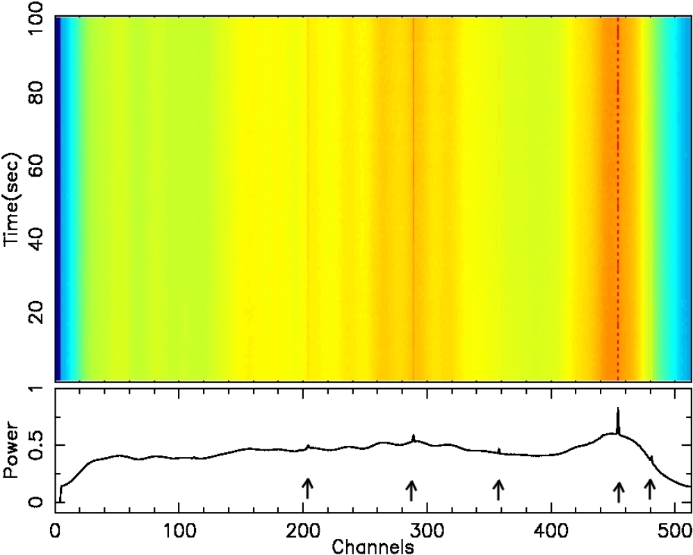
Figure 3.2.: Raw data with the 33 MHz bandwidth divided into 512 channels at 325 MHz, obtained from the GMRT. The top panel shows the observed frequency band power in a colour ramp from blue to red. The band is shown for around 100 seconds of data. The bottom panel shows the average band obtained after averaging 100 seconds of the observed data. The narrow band RFI lines are clearly visible in both the panels and also tagged with arrows in the bottom panel.

3.5.1.2 Single pulses from different observatories

The single pulses from different observatories were obtained using slightly different techniques. For all of the single pulse analysis reported in this thesis, the SIGPROC single pulse file format was used. Hence, a conversion is required at an initial stage for the different formats of the data from different observatories to the selected SIGPROC format.

The GMRT data were recorded in the raw filterbank mode with the header information stored in the separate manually written log files. A conversion was required at this stage into the standard SIGPROC filterbank format from the raw GMRT filterbank data format. For the GMRT data, we used following set of codes to obtain the single pulses.

• Filterbank converts the raw GMRT pulsar data into a SIGPROC filterbank format. The code acquires the necessary details, regarding the observations, by a manual entry before the conversion. In the SIGPROC filterbank format, the data are arranged in the multiple frequency channels per sample with the observations details in the header.

• Dedisperse combines frequency channels after adjusting the dispersion delay between them caused by the interstellar medium. This delay was calculated using the DM of the pulsar obtained from the ATNF catalogue Manchester et al. (2005). The dedisperse time-series consists of samples separated by the effective integration time.

• Fold is the program which folds the SIGPROC time-series data to the given pulsar period. The period can be given manually as one of the input arguments or it can be provided as a polyco file. The polyco file is generated from a publicly available package called TEMPO. The TEMPO code, calculates the pulse arrival time at a given observatory using the known pulsar period and period derivatives and, where necessary, one of the several binary models. The polyco file is the prediction regarding the pulse phase behaviours in a given time range, which are calculated from the input models. The Fold program allows the user to choose the output to be produced in the single pulse format or in the integrated profile format. Fold was also used to bin the time-series in the user defined number of phase bins for each single pulses. For most of the pulsars in this thesis, the period was divided into 256 phase bins.

The WSRT data were obtained as 8 dedisperse time-series from the 8 observed subbands for each pulsar. A separate conversion code was needed to combine these 8 subbands and form a single time-series in the SIGPROC format for the Fold program. The code data${\_}$converter.c, combines these time-series with the respective DM to produce a single dedisperse time-series in the SIGPROC format with the 160 MHz bandwidth. These SIGPROC time-series were folded using the Fold program, using the polyco files, to obtain the single pulses.

At the the Effelsberg telescope, the PSRFFTS recorded data in the SIGPROC filterbank format only. Hence, these filterbank files were directly used to obtain the dedisperse time-series using the appropriate DMs. These SIGPROC time-series were also folded using the Fold program, utilising the polyco files, to obtain the single pulses.

The Arecibo telescope data were converted in the EPN format at the observatory. A separate code, EPN_to_sigproc.c was implemented to convert the observed single pulses with the calibrated polarisations into four separate single pulse files corresponding to the four Stoke’s parameters, I, Q, U and V.

3.5.2 RFI removal from single pulses

After obtaining the single pulses, NF of the pulsar can be obtained. In many occasions, the data show broadband RFI, where the RFI is present for short duration in time but over the entire observed band. These RFI mask the true intensities of the pulses and hence a judgement on the true nature of the pulse, to be either a null or a burst, can not be made. Thus, it is necessary to remove these RFI infected single pulses before the NF analysis. To carry out this task automatically on the observed single pulse files, a code rfi_singlepulse.c was implemented.

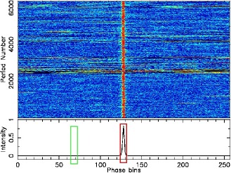
Figure 3.3.: Single pulses from PSR B0835$-$41, observed from the GMRT at 610 MHz. The top panel shows stack of single pulses in a color ramp intensity from blue to red. The bottom panel show the integrated profile, obtained from all the observed pulses. The red square shows the on-pulse window while the green square displays the off-pulse window.

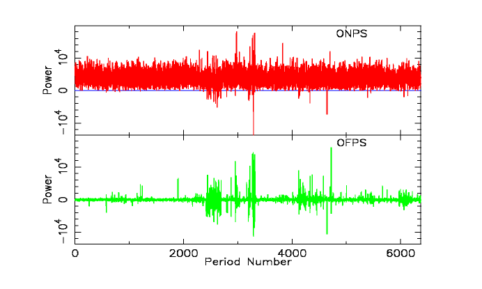
Figure 3.4.: The pulse energy sequence obtained from PSR B0835$-$41. The top panel shows the on-pulse energy sequence while the bottom panel shows the off-pulse energy sequence.

Figure 3.3 shows the single pulses obtained from PSR B0835$-$41 observed from the GMRT at 610 MHz. To identify RFI infected pulses, we selected two windows on the phase bins. The on-pulse window (shown with a red square in Figure 3.3) bounds the entire pulse region. All the phase bins inside this windows were averaged to obtain the on-pulse energy sequence (ONPS). Similarly, equal number of phase bins were selected, away from the main pulse, to form an off-pulse window. All the phase bins, inside the off-pulse window, were added to form the off-pulse energy sequence (OFPS). A baseline was selected (from the remaining phase bins) to obtain the mean counts in the entire off-pulse region, and subtracted for every period. The off-pulse is a region where one does not expect any emission. Hence, for the periods, where a baseline has been subtracted, the OFPS should show distribution around zero mean energy. Figure 3.4 shows the ONPS and OFPS for PSR B0835$-$41. The presence of RFI can be seen in the OFPS, for periods around 2500, where the OFPS fluctuations are larger. To identify these periods, a model root-mean-square (rms) deviation of the off-pulse mean energy was calculated from the periods where such large fluctuations were not present (for example periods between 1500 to 1600 in Figure 3.4). A threshold was adapted as 2 to 3 times the model rms to identify all the pulses which showed mean off-pulse energy beyond this range. All the pulses which were above such threshold were removed from the single pulse data. After removal of these pulses, the remaining pulses were used for the NF analysis.

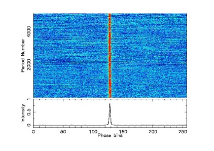
Figure 3.5.: Single pulses from PSR B0835$-$41 at 610 MHz similar to Figure 3.3. All the identified RFI pulses, which showed large fluctuations of the mean off-pulse energy, were tagged and removed.

For most of the observations, the threshold technique was useful to remove the RFI pulses, however for certain observations, the occurrence of RFI were short and did not overlap with the off-pulse window. Hence, it was not possible to remove them using the above mentioned strict threshold. We carried out a visual inspection of the single pulse data to identify such pulses and they were removed manually for a few pulsars. Figure 3.5 displays a stack of single pulses from PSR B0835$-$41 after the removal of all RFI infected pulses. The drawback in removing the RFI infected pulses is the break in continuation of the observed pulse sequence. Hence, these data sets were not used to obtain the null length and the burst length statistics.

3.5.3 Nulling fraction estimation

In this section, the method to estimate the NF is explained in detail. It is similar to the methods used by Ritchings (1976) and Vivekanand (1995) [as mentioned in Section 2.3.1]. The single pulses observed from the PSR B2319+60 at 610 MHz from the GMRT is shown in Figure 3.6. The on-pulse and the off-pulse windows were selected from the integrated profile. The total energy in the on-pulse window and the off-pulse window were calculated for each pulse to form the ONPS and the OFPS. Figure 3.7 presents the obtained ONPS and the OFPS from PSR B2319+60. The presence of nulling can be seen for pulses near the zero pulse energy.

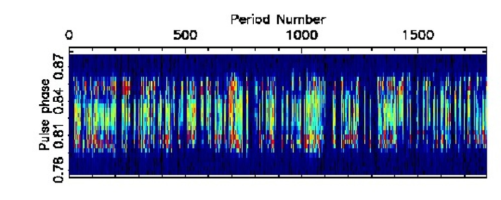
Figure 3.6.: A small section of the single pulses observed from PSR B2319+60 at 610 MHz from the GMRT. The intensities are shown in a color ramp from blue to red. Presence of null pulses can be seen between the burst pulses.

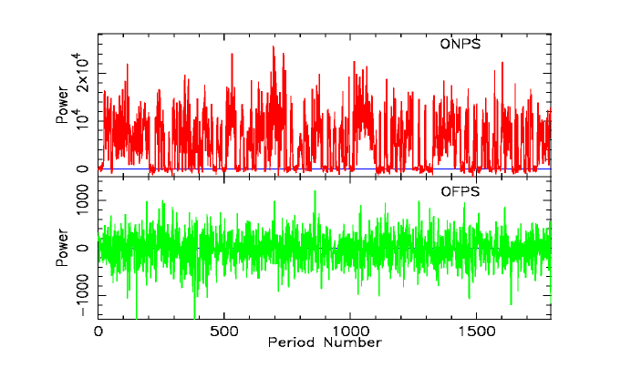
Figure 3.7.: The top panel shows the ONPS while the bottom panel displays the OFPS obtained from PSR B2319+60 observed from the GMRT at 610 MHz. Both the panels show power (in arbitrary units) as a function of period number. The ONPS shows pulses reaching the zero pulse energy, which can be classified as null pulses.

In a few pulsars, the interstellar scintillation can cause the on-pulse energy to fluctuate on a larger scale. The effects of such large fluctuations can be addressed by averaging pulse energy in blocks of around 200 pulses. This technique is introduced briefly in Section 1.3.3. Every pulse in the ONPS and the OFPS were normalised by the average energy estimated for the corresponding block of 200 pulses. The ONPS and the OFPS were binned to various energy bins depending upon the available S/N. The histograms of the on-pulse and the off-pulse energy, after a normalisation by the highest number of occurrence, are shown in Figure 3.8 for PSR B2319+60 (The highest number of occurrence count is always at the zero mean energy bin of the off-pulse energy histogram for a nulling pulsar). It should be noted that, histograms with these normalisation do not give probability distribution, however, choice of such normalisation makes it easier to discern the NF from the histograms.

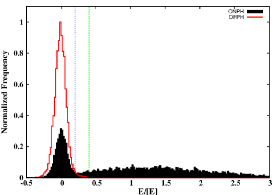
Figure 3.8.: Normalized histograms of the on-pulse and the off-pulse energies as a function of mean pulse energy, [E], for PSR B2319+60. The blue dotted vertical line is a visually selected threshold at the point where null and burst pulse distribution crosses each other (around 0.2 E/[E]) in on-pulse histogram. The green dotted line is a relatively higher threshold (around 0.4 E/[E]) set around the point where the off-pulse energy distribution terminates (see text).

To obtain the NF for each pulsar, modelling of the on-pulse energy histogram (ONPH) and the off-pulse energy histogram (OFPH) were carried out (using the NF.c code). The OFPH represents the telescope noise (a Gaussian random noise), the width of which can be used to estimate the rms fluctuations of the data. During the period, when the pulsar goes into a null state, the on-pulse energy also represents the telescope noise similar to the off-pulse energy. The height of the zero centred energy in the ONPH provides the fraction of the pulses in the null state. If nulling is very prominent, then the ONPH would be indistinguishable from the OFPH due to the large fraction of the null pulses. Pulsar with a steady power output, tends to show a bimodal distribution in the ONPH with two peaks, one at the zero energy bin and other at the mean pulse energy bin. Figure 3.8 shows such bimodal distribution with two peaks in the ONPH for the PSR B2319+60. Both the histograms were normalised by the maximum number of occurrence, at the zero mean energy bin, from the OFPH. As mentioned earlier, such normalisation was adapted to discern the NF directly from the plot. The height of the ONPH, near the zero mean energy bin, represents the fraction of pulses in the ONPH which are similar to the OFPH. This fraction represents the observed nulled pulses in the data, also known as the NF. A scaled version of the OFPH was modelled for the ONPH to estimate this fraction. The ONPH is contaminated with noise which has distribution similar to OFPH distribution. Hence, before subtraction, OFPH has to be deconvolved from the ONPH. However, Ritchings (1976) has reported that such deconvolution does not provide significantly different results. Hence, no such deconvolution was carried out in the analysis of our data. Before the subtraction, the OFPH was modelled as a zero centred Gaussian function, also represented as,

$$G(x)~{}=~{}A\times e^{-(x/C)^{2}}.$$ (3.7)

Here, A is the height of the histogram at zero mean energy, in the units of fraction of pulses, which can be identified as A_OFPH. The rms noise of the system can be estimated from the width of the fitted Gaussian (i.e. C = $\sqrt{2}\times rms$). In the ONPH, the zero energy excess represents the nulled pulses. The height of which can be estimated by fitting the similar Gaussian function given by equation 3.7. Fitting this function on the ONPH provided the a width of the Gaussian function (i.e. C) obtained from OFPH. This parameter was kept fixed in the later fitting process on the ONPH. Thus, only height was used as a free parameter for fitting the ONPH around the zero mean energy bin. This fitting gave an estimation of the A_ONPH. The ratio of the parameters, obtained from the ONPH (A_ONPH) to the one obtained from the OFPH (A_OFPH), states the NF of a pulsar as,

$$NF~{}=~{}\frac{A_{ONPH}}{A_{OFPH}}~{}\times 100\%.$$ (3.8)

The fitted parameters A_ONPH and A_OFPH will have the corresponding fitting errors on them. The error on the NF was obtained using these fitting errors as,

$$\bigtriangleup{NF}=\frac{A_{OFPH}\times(\bigtriangleup{A_{ONPH}})-A_{ONPH}\times(\bigtriangleup{A_{OFPH}})}{(A_{OFPH}^{2})}~{}\times 100\%.$$ (3.9)

Here, $\bigtriangleup$NF is the error on the NF while $\bigtriangleup{A_{ONPH}}$ and $\bigtriangleup{A_{OFPH}}$ are the fitting errors on the $A_{ONPH}$ and $A_{OFPH}$, respectively. For a few pulsars, the null pulse distribution and the burst pulse distribution were not well separated in the ONPH. Hence, fitting the Gaussian on these histograms can give large fitting errors. For these pulsars, where the null and the burst pulse distributions are indistinguishable in the ONPH, the estimation of the NF using the above mentioned method leads to an overestimation. This happens due to the low S/N burst pulses mixing with the null pulse distribution in the ONPH. For pulsars with low S/N burst pulses and relatively good amount of null pulses, consecutive pulses (around 5 to 10 pulses depending upon the single pulse S/N) can be sub-integrated to get the bimodal distribution in the ONPH. Estimation of the NF from the sub-integrated pulses leads to a underestimation, as it is likely that sub-integration will combine few null pulses with the neighbouring burst pulses. Hence, the above mentioned methods has to be used with precautions on the individual cases.

3.5.4 Separation of null and burst pulses

The null and the burst pulses need to be separated in order to carry out further analysis. There are different ways in which these pulses can be separated. We have at large used two different methods in various different cases depending upon the available S/N. A simplest method is to apply a visual threshold on the ONPH as shown in Figure 3.8. This threshold is selected at the location where the null pulse and the burst pulse distributions cross each other. Pulses below the threshold can be identified as the null pulses, while the pulses above the threshold can be tagged as the burst pulses. For pulsars with high S/N burst pulses, such threshold can be set very easily. However, separation using such threshold can lead to erroneous results for the pulsars where the bimodal distributions of ONPH, from the null and the burst pulses, are not well separated. For such ONPH, a threshold can cause a few null pulses to get mix with the separated burst pulses. Similarly, a few low S/N burst pulses can also get mix with the separated null pulses. Hence, for such cases we undertook a slightly different approach.

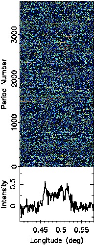
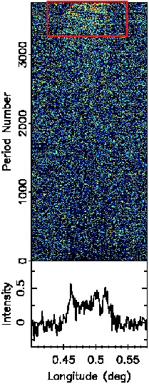
Figure 3.9.: The separated null pulses after applying a slightly higher threshold. The top panels in both the plots show the single pulses while the bottom panels show the integrated profiles. (a) All the separated pulses below the threshold. Note that, it is difficult to identify burst pulses from the single pulses, however a significant integrated profile can be seen, indicating the presence of numerous weak burst pulses. (b) Arranged single pulses in the ascending order of their on-pulse energy. The burst pulses with a relatively higher S/N can be seen towards the high energy end (inside an indicative red square)

A relatively higher threshold was set initially on the ONPH histogram, to separated strong burst pulses above the set threshold (around 0.4 E/[E] in the ONPH of Figure 3.8). The set higher threshold obviated any possibility of null pulses mixing with the high S/N burst pulses. The pulses below such threshold will have a mixture of true null pulses and weak burst pulses as shown in Figure 3.9(a). They show a significant integrated profile indicating the presence of weak burst pulses. To separate these pulses robustly, we calculated the on-pulse energy for every period after weighting the on-pulse bins, for every period, with the average pulse profile. We arranged all these pulses in the acceding order of their on-pulse energy. Such arrangement will cause few pulses, with pulse shape resembling the average profile and having high on-pulse energy, to move towards the high energy end. A box can be selected, as shown in Figure 3.9(b), which encloses all the significant burst pulses at the high energy end. To include most of the weak burst pulses, the lower end of the box was moved from the high energy end towards the low energy end till the pulses outside the box did not show a significant profile (S/N $\sim$ 1). Pulses outside this box were tagged as the null pulses while the pulses inside the box were tagged as the burst pulses. After this final separation, the integrated profiles obtained from the null pulses and the burst pulses are shown in Figure 3.10.

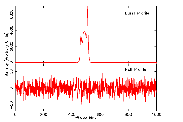
Figure 3.10.: The null and the burst pulse profiles obtained after final separation of the corresponding pulses for PSR B2319+60 observed from the GMRT at 610 MHz. The null pulse profile does not show any significant emission component.

3.5.5 Estimation of the reduction in the pulse energy

The degree by which the radio emission from a nulling pulsar declines during the nulls can be obtained from the average null pulse and the burst pulse profiles of the pulsar for the null and the burst pulses respectively. We calculated the reduction parameter, $\eta$, for a pulsar in a manner similar to that described by Vivekanand & Joshi (1997). First, the total energy from the on-pulse bins of the burst pulse profile was obtained. The rms deviation was obtained from the phase bins inside the predefined on-pulse window of the null pulse profile. To estimate an upper limit on any possible emission inside the on-pulse phase bins, in the null pulse profile, three times the corresponding rms estimate was used. The ratio between the total on-pulse energy of the burst pulse profile and an upper limit on any detectable emission from the null pulse profile can be defined as,

$$\eta~{}=~{}\frac{\sum\limits^{N}_{i=1}P_{bpulse}(i)}{3\times rms_{npulse}}.$$ (3.10)

Here, $P_{bpulse}(i)$ is the intensity of the i^th bin inside the on-pulse window of the burst pulse profile, rms_npulse is the rms estimated over the on-pulse window of the null pulse profile and N is the total number of bins in the on-pulse window. The error on the estimated factor, $\bigtriangleup\eta$, was obtained as three times the off-pulse rms of the burst pulse profile. The $\eta$ robustly quantifies the reduction in the pulse energy during the null state. It can be used to constrain various hypothesis regarding the nulling phenomena.

3.5.6 Null length and burst length histograms

To estimate the distributions of null and burst durations, the null length and the burst length histograms were obtained. For each pulsar, single pulses were tagged with an index number according to their order of occurrence in the observed sequence. The null and the burst pulses were separated as explained in Section 3.5.4. The original index numbers, which remained unaltered after the separation, were used to find a continuous sequence of consecutive null and burst pulses. Figure 3.11 displays a small section of the observed data with their identified emission states (null or burst). To carry out various fluctuations analysis, each null pulse was tagged as zero and each burst pulse was tagged as one [as discussed in Section 2.3.1, Backer (1970c) introduced this technique]. Thus, from the identified state sequence of the pulses, a onezero time-series was formed (as shown in Figure 3.11). A Fourier transform of such one-zero series can be used to scrutinize periodicities associated with the nulling phenomena.

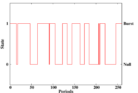
Figure 3.11.: A sequence of pulses with their corresponding identified null/burst state for PSR B2319+60 observed at 610 MHz. All the null pulses were tagged as zeros and all the burst pulses were tagged as ones.

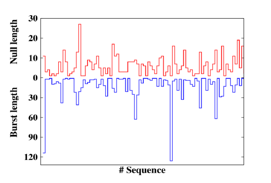
Figure 3.12.: A section of the observed null length and the burst length sequences for PSR B2319+60. The red solid line shows the observed null length sequence. The bottom solid blue line shows the length of bursts succeeding the null shown at the top for each step. The ordinate scale for both the sequences are different to display them in a same plot.

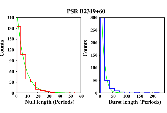
Figure 3.13.: The observed null length and the burst length histograms from PSR B2319+60. The exponential fits are shown with a green solid lines. Note the clear exponential decay in the frequency of occurrence from shorter lengths to longer lengths in both histograms.

An individual uninterrupted sequence of null (or burst) pulses can be used to count the length of the corresponding null (or burst) state in the units of number of pulses. A nulling pulsar switches between the null state and the burst state with different time-scales. From the identified emission state sequence, such as Figure 3.11, a sequence of consecutively occuring null lengths and burst length can also be formed. Figure 3.12 shows a small section of consecutive null lengths and burst lengths for PSR B2319+60. It can be seen from Figure 3.12, the pulsar exhibits various lengths of null and burst phases. It should be noted that, for the in case of lower S/N, identification of true null and burst pulses can become difficult task. It can cause large differences in the obtained null length and burst length histograms, specially near the short nulls short bursts. Cordes (2013) has presented a compahensive study on this aspect.

These null length and burst length sequences were binned to form the null length histogram (NLH) and the burst length histogram (BLH). A few pulsars exhibit large fraction of RFI infected pulses, where a judgement regarding the pulse emission state can not be made. For these pulsars, null lengths and burst lengths, which include RFI infected pulses, were entirely excluded. Figure 3.13 displays the obtained null length and burst length histograms for PSR B2319+60. The distributions follow an exponential slope with relatively higher number of short null/burst lengths. As discussed in Section 2.4.2, its important to investigate the time-scale of these length distributions to scrutinize various nulling mechanism models. They are discussed further in Section 4.5.

3.5.7 Longitude resolved fluctuation spectra

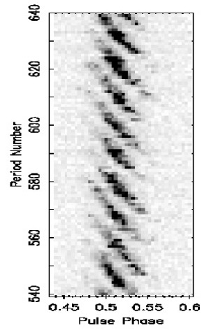
Figure 3.14.: A composite plot of the Longitude resolved fluctuation spectra. (a) A section of the single pulses observed from PSR B0809+74 at 610 MHz. The drifting of the subpulses is clearly visible. (b) The phase-resolved fluctuation spectra obtained from the single pulses displayed in (a). The center panel shows a contour plot of the spectra over the given phase bin range. The left side panel shows the integrated profile. The bottom panel shows the combined spectrum after averaging the above spectra over the on-pulse longitude. A clear spectral feature with 11 period periodicity is visible in the average spectrum and also in the contour plot.

Many pulsars in our sample do exhibit regular drifting behaviour. Section 1.5.2 introduced this phenomena, while a detail discussion regarding its origin in presented in Section 2.2.2. To identify the drifting periodicities, we obtained a Longitude resolved fluctuation spectra (LRFS). The LRFS represents a Fourier transform computed over each individual phase bin in a contour plot. Figure 3.14(a) shows a section single pulses from a very prominent drifting pulsar, PSR B0809+74. To obtain the drifting periodicity, the pulsar period was divided into 256 phase bins (512 bins in a few cases). Pulse-to-pulse fluctuation time-series was obtained for the individual phase bin. A Fourier transform was carried out for each phase bin time-series to identify the fluctuation periodicities. The obtained Fourier spectra from all the phase bins were displayed in a contour plot to highlight the common features over the on-pulse phase bins. If a pulsar exhibit regular drifting behaviour, then the contour plot will show peak at the corresponding periodicity only at the on-pulse phase bins. An example of such composite LRFS for PSR B0809+74 is shown in Figure 3.14(b). The central panel in Figure 3.14(b) shows the contour plot of the Fourier spectra obtained from all the phase bins. The peaks in the contour plot and a strong peak in the average spectrum located near 0.09 cycles/period which corresponds to drifting periodicity of around 11 periods. The drifting periodicity, also clearly visible in Figure 3.14(a), is consistent with the reported periodicity by Lyne & Ashworth (1983).

Chapter 4 A survey of nulling pulsars using the GMRT

4.1 Introduction

Pulsar nulling is reported to occur in around 109 pulsars (see Table LABEL:table_all_null_psr). NF, as discussed in Section 3.5.3, is a widely used quantity to measure the degree of nulling in these pulsars. However, NF does not specify the duration of individual nulls, nor does it specify how the nulls are spaced in time. Although some attempts of characterising patterns in pulse nulling were made in the previous studies Backer (1970c); Ritchings (1976); Janssen & van Leeuwen (2004); Kloumann & Rankin (2010), not many pulsars have been studied for systematic patterns in nulling, partly because these require sensitive and long observations.

Recent discoveries suggest that nulling pulsars with similar NF may have different null durations. These include intermittent pulsars, such as PSR B1931+24 Kramer et al. (2006) and PSR J1832+0029 Lyne (2009), and the RRATs, which show no pulsed emission between single burst of emission McLaughlin et al. (2006); Keane et al. (2011)[see Section 2.3.5 for details]. These pulsars also show extreme degree of nulling similar to a few classical nulling pulsars. As mentioned in Section 2.3.5, PSR B1931+24 exhibits radio pulsations for 5 to 10 days followed by an absence of pulsations for 25 to 35 days Kramer et al. (2006). If the cessation of radio emission in this pulsar is interpreted as a null, it has a NF of about $\sim$72 to 85% similar to PSR J1502$-$5653 Wang et al. (2007); Li et al. (2012). Yet the latter shows nulls with a typical duration of few tens of seconds in contrast to a much longer duration for PSR B1931+24. A similar conclusion can be drawn by comparing RRATs with classical high NF pulsars. While this leads to the expectation that pulsars with similar NF may have different nulling time-scales, no systematic study of this aspect of nulling is available to the best of our knowledge. In this chapter, a modest attempt to investigate this is initiated.

Pulse nulling was usually believed to be a random phenomenon Ritchings (1976); Biggs (1992). However, recent studies indicate a non-random nulling behaviour for a few classical nulling pulsars Herfindal & Rankin (2007b, 2009); Redman & Rankin (2009); Kloumann & Rankin (2010) [see Section 2.3.3 for details]. Redman & Rankin (2009) also report random nulling behaviour for at least 4 out of 18 pulsars in their sample. Therefore, it is not clear if non-randomness in the sense defined in Redman & Rankin (2009) is seen in most nulling pulsars and such a study needs to be extended to more nulling pulsars. This issue is investigated in this chapter with a distinct set of nulling pulsars.

In this chapter, we present observations of 15 pulsars, carried out using the GMRT at 325 and 610 MHz. Among these, five were discovered in the PKSMB survey Manchester et al. (2001); Morris et al. (2002); Kramer et al. (2003); Lorimer et al. (2006), which have no previously reported nulling behaviour. Selection of these pulsars is justified in Section 3.3. Rest of the sample consists of well known strong nulling pulsars. The observations and analysis techniques are similar to the one described in Chapter 3. In Section 4.2, nulling behaviour for individual pulsar is discussed along with estimates of their NFs and the reduction in the pulsed energy during the null state. A comparison of the null length and burst length distributions for pulsars, which have similar NF, is presented in Section 4.3 and a discussion on the randomness of nulls is presented in Section 4.4. The expected time-scales for the null and the burst durations are presented in Section 4.5. Finally, the conclusions are presented in Section 4.6 while the implications of these results are discussed in Section 4.7.

4.2 Single pulse behaviour of individual pulsars

The on-pulse and the off-pulse energy histograms for each observed pulsar are shown in Appendix A. The null and the burst pulses were separated, using the method discussed in Section 3.5.4, for each pulsar. The separated null and burst pulses were used to construct the null length histograms and the burst length histograms, shown in Appendix B.

B0809+74

As mentioned in Section 2.3.1, this is one of the well studied nulling pulsar. Nulling in this pulsar was first reported by Taylor & Huguenin (1971). A section of observed single pulses at 325 MHz, is shown in Figure 4.1(a), which displays a clear null region around period number 440. An upper limit on NF for this pulsar was estimated by Ritchings (1976). A refined value of the NF was estimated by Lyne & Ashworth (1983) using 40 hrs long observations. Lyne & Ashworth (1983) also reported reduction in burst pulse energy by $>$ 78 times. This is the only pulsar in the sample with a previously reported $\eta$ value. The on-pulse and the off-pulse energy histograms obtained from our observations are shown in Figure A.1. The ONPH shows clear bimodal distribution originating due to small fraction null pulses and large fraction of strong burst pulses. We obtained the NF of 1.0$\pm$0.4% using these histograms. The estimated $\eta$ is 172.0$\pm$0.5, which matches with the previously reported lower limit by Lyne & Ashworth (1983). Figure B.1 shows the NLH and the BLH, constructed using 73 null lengths and 73 burst lengths. The NLH shows typical null length of around 1 to 3 periods occurring more frequently while extending the overall distribution up to 8 periods null. The BLH shows exponentially declining distribution of burst lengths up to 800 periods. We also carried out LRFS analysis (shown in Figure 4.2) to highlight the 11 period periodicity, confirming the earlier claims by Lyne & Ashworth (1983) and van Leeuwen et al. (2002). The pulsar also shows intriguing change in the drift rates before and after the null states Lyne & Ashworth (1983); van Leeuwen et al. (2002).

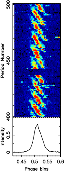
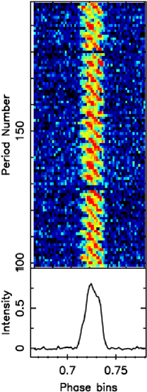
Figure 4.1.: Sections of observed single pulses from three pulsars namely, PSRs (a) B0809+74 (b) B0818$-$13 (c) B0835$-$41. The top panel in all sub-plots shows stack of 100 pulses with pulse intensity displayed in a color ramp from blue to red. The bottom panel in each sub-plot presents the respective integrated profile. Presence of null pulses are clearly evident for all three pulsars in addition to clear drifting of subpulses in PSRs B0809+74 and B0818$-$13.

Figure 4.2.: Phase-resolved fluctuation spectra obtained from the observed single pulses at 325 MHz of PSR B0809+74. The centre panel shows a contour plot of the spectra over the given phase bin range. The left side panel shows the integrated profile. The bottom panel shows the combined spectrum after averaging the above spectra over the on-pulse bins. A clear spectral feature with 11 period periodicity is visible in the average spectrum and also in the contour plot.

B0818$-$13

Figure 4.3.: Phase-resolved fluctuation spectra obtained from the single pulses of PSR B0818$-$13 (see Figure 4.2 for details regarding various panels). The drifting feature of around 0.21 cycles per period is clearly evident which corresponds to 4.8 period periodicity.

This is one of the well known nulling pulsar. A section of observed single pulses at 610 MHz is shown in Figure 4.1(b) which shows clear null pulses at period numbers around 130 and 180. Lyne & Ashworth (1983), did an extensive study about the change in the drift pattern before and after the null states in this pulsar (see Section 2.3.1). Our data show drifting feature at 0.21 cycles per period (Figure 4.3) which matches with the earlier reported P₃ Lyne & Ashworth (1983); Janssen & van Leeuwen (2004). The pulse energy histograms are shown in Figure A.2. Our NF (0.9$\pm$1.8%) also matched with the earlier reported NF (1.01$\pm$0.01%) within the error bars. The new result from our study is the amount of flux reduction during the null states. Although this is a relatively stronger pulsar, the estimated $\eta$($\sim$ 4.2) is comparatively small. The NLH and the BLH are shown in Figure B.2, which were constructed using 57 null lengths and 57 burst lengths. The NLH shows around 90% of nulls tend to occur for only single period while the rest 10% are distributed up to 4 periods. The BLH shows smooth exponential decline of the burst lengths distribution up to 400 periods.

B0835$-$41

Nulling in this pulsar was first reported by Biggs (1992). A section of observed single pulses at 610 MHz is shown in Figure 4.1(c), which shows regions of short null states around period numbers 100 and 140. The on-pulse and the off-pulse energy histograms are shown in Figure A.3. The estimated NF, of around 1.7$\pm$1.2%, is small like in the case of PSR B0818$-$13. However, estimated $\eta$ (15.7$\pm$0.2) is comparatively higher. The NLH and the BLH are shown in Figure B.3, which were constructed using 74 null lengths and 74 burst lengths. The NLH shows very interesting null length distribution as more than 95% of the nulls tend to occur only for one period, while the rest 5% tend to occur for two periods. It can be speculated that the true nulling time-scale could be shorter than the period of the pulsar and the observed NLH presents only a tail of this distribution. The BLH shows exponentially declining distribution of burst lengths up to 500 periods.

B1112+50

For this pulsar, nulling was first reported by Ritchings (1976). This pulsar was reported to have three different profile modes of emission at 1420 MHz Wright et al. (1986), where it shows two distinct profile components. In this survey, observation at 610 MHz showed single profile component. The pulsar shows sporadic nature of pulse energy modulations. The pulse energy histograms are shown in Figure A.4, using which the NF of around 64$\pm$6% (which matches with the reported NF of around 60$\pm$5% by Ritchings (1976)) was obtained. For the large fraction of the observed duration, pulsar switched rapidly between the null state and the burst state within one or two periods. The reduction in the pulse energy, $\eta$, during these null states is 44.7$\pm$0.2. Due to the intriguing flickering nulls seen in Figure 4.4(a), it is interesting to investigate periodicity of this pulse energy fluctuations. However, the obtained LRFS, shown in Figure 4.5, did not show any significant spectral feature, rejecting any possibility of periodicity in the pulse energy modulation. Weltevrede et al. (2007) also reported no strong spectral feature in their observations at 92-cm. Theoretically, it would be challenging to propose any nulling mechanism which can cause changes to the pulse energy by such a large fraction (around 45 times) in such a short time-scale (one to two periods). The overall NLH and the BLH, constructed using 635 null lengths and 635 burst lengths, are shown in Figure B.4. They show large fraction of short nulls and short bursts with exponentially declining null length and burst length distributions up to 50 periods.

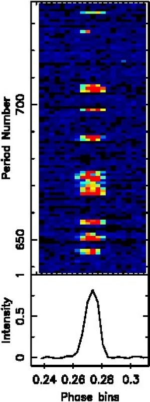
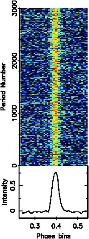
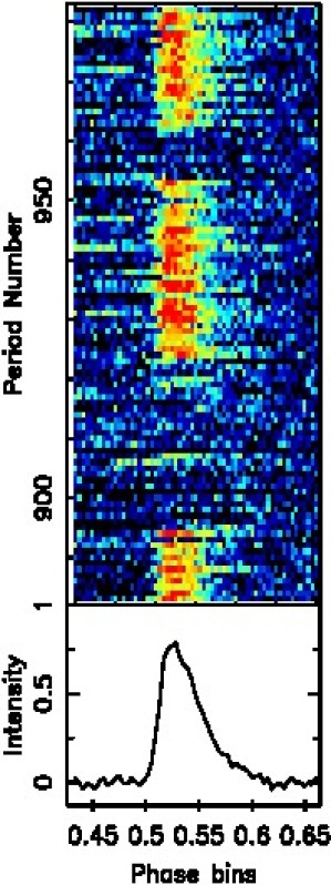
Figure 4.4.: Modulation of the pulse energy for PSRs (a) B1112+50 (b) J1639$-$4359 (c) J1701$-$3726 (see Figure 4.1 for details regarding panels) observed at 610 MHz. For PSR J1639$-$4359, successive 16 periods were sub-integrated as the single pulses were below the detection level. The plot shows the resulting sub-integrations for a section of the observed data. The period range is kept unaltered for comparison.

Figure 4.5.: Phase-resolve fluctuation spectra for PSR 1112+50 (see Figure 4.2 for details regarding various panels). The spectra is featureless with absence of any significant periodicity.

J1639$-$4359

This is one of the newly discovered pulsars from the PKSMB survey Kramer et al. (2003). The single pulses from this pulsar were very weak. The single pulse data were averaged over successive pulses to form average profiles for every block of 16 single pulses (sub-integration) to show the pulse energy modulations. The pulse sequence of around 180 sub-integrated blocks (3000 pulses) is shown in Figure 4.4(b). As its clearly evident from the sub-integrated pulse plot, there are no clear null states. Figure A.5 shows the on-pulse and the off-pulse energy histograms, obtained from the sub-integration of successive 16 periods. The histograms are presented just to demonstrate the absence of null pulses among the sub-integrated pulses. Estimation of the NF was not possible as averaging over consecutive periods resulted in detection of emission for every sub-integration giving a NF of zero (as shown in Figure A.5). However, some of the single pulses in a sub-integration may well have been nulled pulses. To estimate an upper limit on the fraction of such pulses for this pulsar, we arranged all the single pulses in the ascending order of their on-pulse energy. A threshold was moved from the lower energy end towards the high energy end till the pulses below the threshold did not show a significant (S/N $>$ 3) profile component (similar to the method discussed in Section 3.5.4). These pulses, located below the threshold at the lower energy end, were tagged as the null pulses. Although, it is likely that these pulses are a mixture of true null pulses and weak burst pulses (as the expected significance was comparatively higher with S/N $>$ 3 compared to such threshold mentioned in Section 3.5.4). Hence, the fraction of these pulses were used only as an upper limit of around 0.1%, as the true NF for this pulsar could be lower than this limit, if more sensitive observations are conducted. The NLH and the BLH were not possible to obtain as the pulsar showed weak single pulses.

B1658$-$37

Nulling in this pulsar was first reported by Wang et al. (2007) with a lower limit on the NF ($>$14%). It was also reported to have short nulls. However due to lower S/N, Wang et al. (2007) sub-integrated 10 pulses. Our observations were more sensitive with higher S/N on single pulses [shown in Figure 4.4(c)], hence we obtained better estimate on the NF (22$\pm$4) compared to earlier reported value. The pulse energy histograms used to estimate this NF are shown in Figure A.6. The null pulses and burst pulses were separated and the obtained length histograms are shown in Figure B.5, which show exponentially declining null length and burst length distributions. The NLH also shows a slight excess of around 10 period nulls. Total 73 null lengths and 73 burst lengths were used to obtain these length histograms. A careful look at the single pulse sequence reveals interesting pulse energy fluctuation with a sudden fall of the pulse energy at the beginning of the null state followed by a gradual rise towards the end. Figure 4.6 shows an example of two consecutive null states which shows a gradual rise of the on-pulse energy towards the end of the null state. This behaviour has been reported for the first time in this pulsar. Wang et al. (2007) reported two different profile modes in this pulsar at 1420 MHz. However, scattering caused by the observations at a lower frequency hindered identification of different profile components. Hence, no profile mode-changing was possible to identify from our observations.

Figure 4.6.: On-pulse energy sequence of around 140 pulses obtained from PSR B1658$-$37 observed at 610 MHz. Two consecutive null regions are shown, with the pulse energy reaching zero, around pulse numbers 1940 and 2000. A sudden drop and a gradual rise of the pulse energy is clearly evident before and after the null states respectively.

J1715$-$4034

This is one of the pulsar discovered in the PKSMB survey Kramer et al. (2003) and it shows single broad integrated profile of more than 15% duty cycle at 610 MHz with a prominent scattering tail. Width of the pulses shows significant modulation as seen in Figure 4.7(a). The pulsar shows two profile components at 1420 MHz Kramer et al. (2003), which is difficult to identify at 610 MHz because of the interstellar scattering. Modulation in these components can cause this apparent change in the pulse width. The estimation of the NF, was obtained after sub-integrating successive 10 pulses. As discussed in Section 3.5.3, such sub-integration will cause few null pulses to merge with the neighbouring burst pulses. Thus, only a lower limit on the NF was possible to obtain using the conventional estimation technique. The pulse energy histograms, used in the estimation of the NF ($\geq$ 10%), are shown in Figure A.7. The pulsar was too weak to obtain the NLH and the BLH.

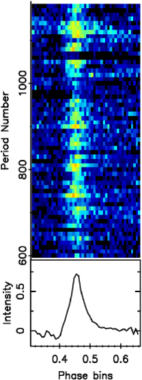
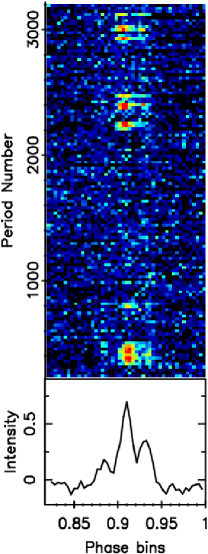
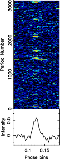
Figure 4.7.: Modulation of pulse energy for three pulsars. Successive 10, 24 and 5 periods were averaged as a sub-integration respectively for PSRs (a) J1715$-$4034, (b) J1725$-$4043 and (c) J1738$-$2330. The period numbers are kept unaltered for comparison. PSR J1725$-$4043 shows weak emission during its long null regions (for example periods between 1000 to 2000). PSR J1715$-$4034 shows rapid modulation of the pulse width while PSR J1738$-$2330 shows burst bunches separated by long null states.

J1725$-$4043

This is also one of the pulsar discovered in the PKSMB survey Kramer et al. (2003) with no previously reported nulling behaviour. Its integrated profile at 610 MHz exhibits three narrow components - one strong central component with weak trailing and leading components. To improve the S/N, 24 successive pulses were sub-integrated. A section of these sub-integrations as well as the integrated profile for this pulsar is shown in Figure 4.7(b). The pulse energy histograms, obtained from the sub-integrated pulses, are shown in Figure A.8, which shows large fraction of null pulses. Visual inspection of the Figure 4.7(b) shows emission bunches of 50 to 200 strong pulses, which correspond to the normal integrated profile [hereafter referred as Mode A - for example periods between 120 to 264 in Figure 4.7(b)]. After adding all the sub-integrations during the null states, separated by a visual inspection, a weak profile [hereafter referred as Mode B - for example periods 264 to 780 in Figure 4.7(b)], different from the normal integrated profile (Mode A), is obtained. The integrated profiles for the two modes are shown in Figure 4.8. Although the two profiles are similar in shape with distinct three components, Mode B profile shows relatively stronger trailing component (Figure 4.8). Table 4.1 shows S/N of various peaks from Mode A and Mode B profiles to compare their significance. Hence, it appears that the pulsar shows sporadic emission with two distinct modes. As the pulses were weak, the NLH and the BLH were not possible to obtain.

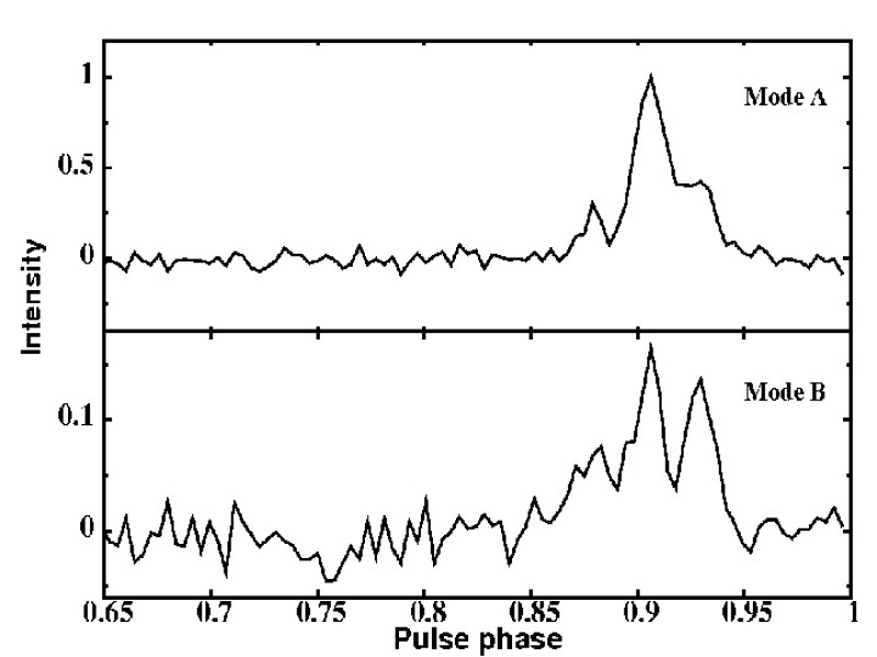
Figure 4.8.: Integrated pulse profiles for Mode A and Mode B of PSR J1725$-$4043. The ordinate is in arbitrary units and was obtained after scaling the two profiles by the peak intensity of the Mode A profile. The Mode B is around 10 times weaker than Mode A.

Component	Mode A	Mode B
Central	37	10
Trailing	15	9

Table 4.1.: Peak S/N for various peaks of Mode A and Mode B profiles. The S/N were calculated using the root mean square deviation from the off pulse regions of respective profiles.

Visual inspection of the single pulses, forming the null sub-integrations, reveals weak individual pulses among nulled pulses. Hence, it is difficult to identify null pulses as these could be low intensity Mode B pulses. The pulsar spends 30% of time in Mode A emission. The remaining 70% could be combination of null pulses and Mode B emission. Hence, only an upper limit on the NF, of around 70% for this pulsar was possible to obtain.

J1738$-$2330

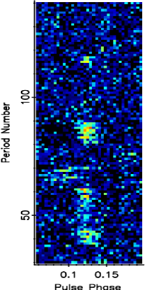
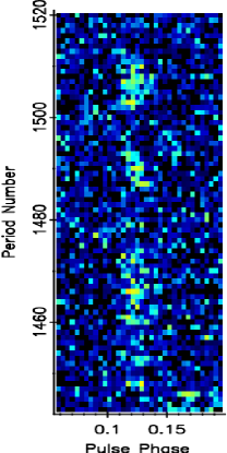
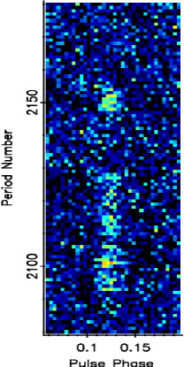
Figure 4.9.: Three example of burst bunches observed at 325 MHz obtained from PSR J1738$-$2330. Note the structure of burst bunches with longer to smaller short bunches, separated by short null states, inside each big bunch. Details regarding this peculiar behaviour are further discussed from longer observations in Chapter 5.

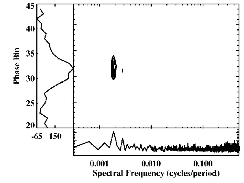
Figure 4.10.: Phase-resolved spectra for PSR J1738$-$2330 (see Figure 4.2 for details regarding panels). The spectra in the bottom panel and in the contours are shown with the abscissa plotted in a logarithmic scale upto the Nyquist frequency.

This pulsar was also discovered in the PKSMB survey Lorimer et al. (2006). We observed this pulsar at 325 MHz using the GMRT. We are reporting a unique nulling behaviour of this pulsar in this chapter. The pulsar seems to have quasi-periodic bursts, with an average duration of around 50 to 100 periods, interspersed with nulls of around 300 to 400 periods. This interesting single pulse behaviour in this pulsar is evident in Figure 4.7(c), where a plot, with 5 successive single pulses integrated, is shown. A visual inspection shows that it seems to have regular periodic bursts for total 1200 periods (bursts at period number 1700, 2100, 2600 and 3100 in Figure 4.7(c)). Figure 4.10 shows the LRFS for this pulsar. It shows quasi-periodicities at nearly 0.0019 cycles per period and 0.0028 cycles per period, which correspond to periodicities of approximately 525 and 350 periods, respectively. Such large periodicities can only occur from a quasi-periodic modulation of the pulse energy. This quasi-periodic behaviour is similar to PSR B1931+24 but with much shorter time-scale. Figure A.9 shows the on-pulse and the off-pulse energy histograms from the sub-integrated pulses. Only a lower limit of around 69% was possible to obtain from these data due to the sub-integration. As the pulses were weak, the NLH and the BLH were not possible to obtain.

Close examination of single pulses suggests that the bursts typically consist of a sequence of a 20 to 30 period bursts followed by 2 short bursts of 5 to 10 pulses. These three bursts are separated by shorter nulls of about 10 to 25 pulses. The overall burst bunches are separated by around 400 periods nulls. Three examples of this burst pattern are shown in Figure 4.9. However, the single pulse S/N was too low to confirm this with high significance. A more sensitive observations, motivated from this study, was carried out and more details regarding this pulsar’s nulling behaviour are discussed in Chapter 5.

J1901+0413

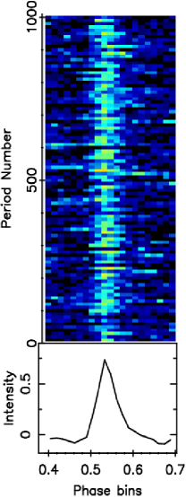
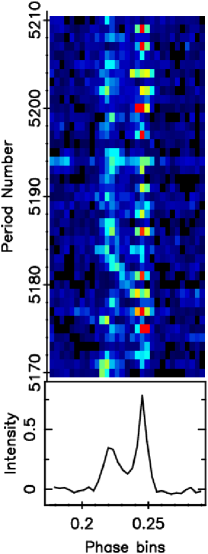
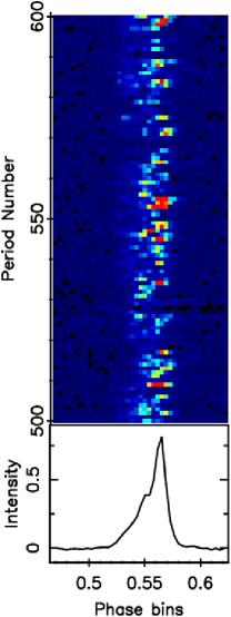
Figure 4.11.: Modulation of pulse energy for PSRs (a) J1901+0413, (b) B2020+28 and (c) B2021+51. For PSR J1901+0413, successive 10 periods were sub-integrated to improve the S/N for this display with period numbers unaltered for comparison. Note the even-odd modulation in the trailing component of PSR B2020+28.

This pulsar was also discovered in the PKSMB survey Morris et al. (2002) with no previously reported nulling behaviour. The pulsar showed single component profile with 15% duty cycle with a prominent scattering tail at 610 MHz [shown in the bottom panel of Figure 4.11(a)]. The single pulses were weak, hence 10 successive single pulses were sub-integrated, as shown in Figure 4.11(a), to display the pulse energy modulation. Visual inspection of the single pulses showed small amount of nulling, hence estimation of the NF using conventional technique was not possible. It was only possible to obtain an upper limit using the similar method discussed for PSR J1639$-$4359. We arranged all the single pulses in the ascending order of their on-pulse energy. A threshold was moved from low to high on-pulse energy end till the pulses below the threshold did not show a collective profile with a pulse with high significance (S/N $>$ 3). All the pulses below such threshold were tagged as null pulses. The fraction of these pulses gave an estimate for the upper limit on the NF ($<$ 6%). As the pulses were weak, the NLH and the BLH were not possible to obtain.

B2020+28

This is one of the well studied pulsar. The pulsar profile shows two strong components [shown in the bottom panel of Figure 4.11(b)], but this pulsar was classified as triple profile class pulsar due the core emission in the saddle region between the two components Rankin et al. (1989). A small section of single pulses is shown in Figure 4.11(b). Interestingly, the emission in the individual profile components reduces significantly for only for a small fraction of pulses, which is different for the two components. A clear even-odd modulation pattern can be seen in the trailing component while the leading component does not show such rapid fluctuations. To scrutinise these modulations, the LRFS was obtained (as shown in Figure 4.12) which clearly shows even-odd modulation in the trailing component. Our results matches with the earlier reported behaviour by Nowakowski et al. (1982). The pulsar shows small amount of nulling when the entire pulse longitude is considered [see Figure 4.11(b)]. The pulse energy histograms are shown in Figure A.11 which shows significantly small number of pulses near the zero pulse energy. We estimated NF of 0.2$\pm$1.6% of for this pulsar. Estimation of the reduction in the pulse energy was around 2.5$\pm$0.2. The large errors in the NF is due to the fewer number of full null pulses in the data. However, there are many pulses which show partial nulls (i.e. null in only one of the component). Our time resolution was not sufficient to identify the saddle region clearly so we were able to estimate the NF for two components only. The estimated NF for the leading component is 3.5$\pm$0.8% and $\eta$ is around 9.7. The estimated NF for the trailing component is 9$\pm$1 % and $\eta$ is around 21, suggesting that at least the trailing component shows a nulling behaviour similar to a regular nulling pulsar. Both the NFs were significantly higher than the overall NF. Due to the small number of full null pulses, the NLH and the BLH were not possible to obtain.

Figure 4.12.: LRFS for PSR B2020+28 (see Figure 4.2 for details regarding panels). The combined spectra shows peak at 0.48 cycles per period, near the alias frequency (Nyquist frequency) which corresponds to periodicity of around 2.1 pulses in the trailing component.

B2021+51

This pulsar was reported nulling by Ritchings (1976) with only an upper limit on the NF($\leq$ 5%). A small section of observed single pulses is shown in Figure 4.11(c). As can be seen from the single pulse plot, we were able to obtain sufficient S/N for single pulses. The pulse energy histograms are shown in Figure A.12. We were able to obtain a better constrain on the NF (1.4$\pm$0.7%). The estimated reduction in the pulse energy, $\eta$ is 2.6$\pm$0.2. The null and burst length histograms are shown in Figure B.6, obtain using 12 null lengths and 12 burst lengths. The NLH shows that 60% of nulls are single period nulls while the rest 40% nulls are double period nulls. This nearly equal distribution between single and double period nulls can be extrapolated to claim small number of shorter nulls (i.e. size smaller than pulsar period) compared to large number of such nulls in PSR B0835$-$41. Such large number of double period nulls, assuming exponential null length distribution seen in most pulsars, suggest the pulsar to have few long nulls (i.e. longer than double period) which are not seen in our data. BLH histogram shows around 65% of burst are less than 100 periods while the distribution extends up to 800 periods.

B2034+19

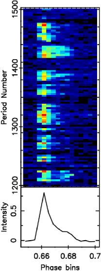
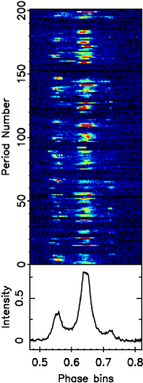
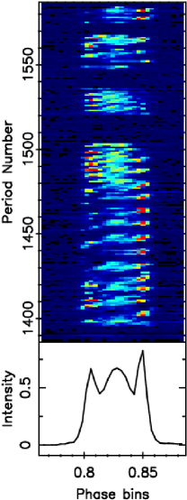
Figure 4.13.: Modulation of the pulse energy for PSRs (a) B2034+19, (b) B2111+46 and (c) B2319+60. For PSR B2034+19, successive 3 periods were sub-integrated to improve the S/N for this display with period numbers unaltered for comparison. PSR B2111+46 shows interesting modulation pattern in its three components, with different components showing independent occurrences of null events for a few periods. PSR B2319+60 clearly shows change in the drift rate around period number 1480 where it also switches the profile modes.

This pulsar was reported nulling by Herfindal & Rankin (2009). We observed this pulsar at 610 MHz and a section of observed pulse sequence is shown in Figure 4.13(a). To improve the S/N, successive 3 periods were sub-integrated. The pulse energy histograms are shown in Figure A.13, obtained using these sub-integrated data. Hence, we were able to estimate only a lower limit on the NF ($\geq$26%). Although, the estimated NF matches with the earlier reported value within the error bars, it is slightly smaller due to our inability to detect short nulls. By arranging pulses in the ascending order of their on-pulse energy and using the variable threshold method discussed in Section 3.5.4, we were able to clearly separate null and burst pulses from the single pulse data. Using these separated null and burst pulses, with estimated $\eta$ of 6.4$\pm$0.1, the obtained null and burst length histograms are shown in Figure B.7. Total 336 null lengths and 336 burst lengths were used to obtain these length histograms. The NLH shows gradual distribution of null lengths up to 10 periods. This is small given that pulsar spends more than 26% of time in the null state. The BLH shows more than 50% of bursts are of size smaller than 3 periods while the other half extends up to 50 periods.

B2111+46

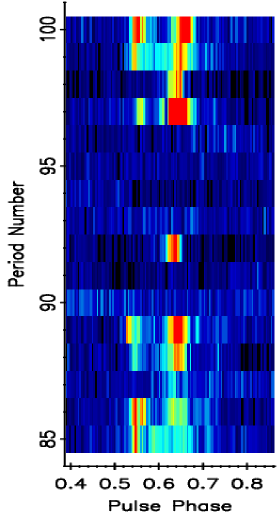
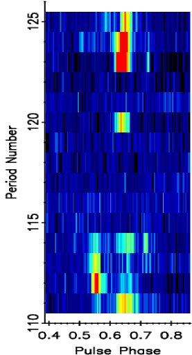
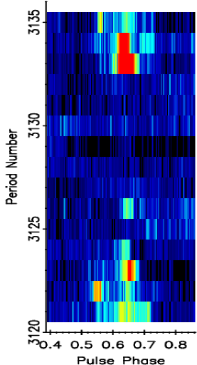
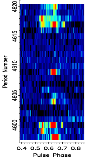
Figure 4.14.: Four example of long nulls seen in PSR B2111+46, observed at 610 MHz. Note the presence of core emission in the individual burst periods inside the long null regions, where both the conal components show clear nulls.

This pulsar is one of the long period well studied pulsar with multicomponent profile [bottom panel of Figure 4.13(b)]. Rankin et al. (1989) classified this pulsar as triple component profile class pulsar but Zhang et al. (2007) reported two additional components in the saddle region connecting the core component and the outer components. The depolarisation shows swing in the middle component at 600 MHz Gould & Lyne (1998), hence, the profile is of core multicomponent class. A section of the observed single pulses at 610 MHz is shown in Figure 4.13(b). Our data shows stronger emission in the saddle region compared to core and outer conal components for many individual pulses. Nulling in this pulsar was first reported by Ritchings (1976). Figure A.14 shows the conventional pulse energy histograms obtained after considering the entire pulse longitude. We measured a slightly higher NF (21$\pm$4%) compared to the previously reported estimate by Ritchings (1976). Like PSR B2020+28, the fraction of pulses for which emission is not detected varies from component to component. For the core component, NF was estimated to be of 26$\pm$2%, slightly higher than the NF of the entire pulse. The estimated $\eta$ value for this component is around 56. For the leading component, NF was found to be 53$\pm$5%, almost double the NF for the entire pulse. The NLH and the BLH, shown in Figure B.8, considering the emission in the entire pulse are reported here for the first time for this pulsar. The NLH shows 50% of nulls are single period nulls while other 50% are gradually distributed up to 10 periods. Total 145 null lengths and 145 burst lengths were used to obtain these length histograms.

Visual inspection of the single pulse data shows many long nulls with lengths varying from 8 to 16 periods. Many of these long nulls show single burst from the core component located inside them. Some of the interesting cases of such nulls are shown in the Figure 4.14. This behaviour has been reported for the first time in this pulsar to the best of our knowledge. It is consistent with the estimated NF of the leading component (around 52%) compared to the NF of the core component (around 26%) as these burst pulses reduce the NF of the core component. However, length of our observations were not sufficient to claim a statistically significant result of this behaviour. Our study motivates longer observations of this pulsar as many of the interesting single pulse behaviour has not been investigated yet.

B2319+60

This is also one the long period well studied pulsar. Pulsar has three component at 610 MHz. It has reported NF of around 25$\pm$5% Ritchings (1976). Observed single pulse data show that this pulsar displays a regular switching between three different profile modes. During two of these modes, it exhibits regular drifting behaviour while in the third mode no such drifting feature is seen. Figure 4.13(c) shows a section of observed single pulses from this pulsar. A clear change in the drift rate (transition from slower drift mode to faster drift mode) is clearly seen around period number 1480. This matches with the reported behaviour for this pulsar at 1 GHz by Wright & Fowler (1981) [also discussed in Section 2.3.2]. More details regarding the broadband nulling behaviour of this pulsar are discussed in Chapter 6. Figure A.15 shows the obtained pulse energy histograms. The estimated NF, using these histograms, is around 29$\pm$1 % and estimated $\eta$ is around 115.8$\pm$0.4 which is second highest in our sample. Figure B.9 shows the exponentially declining length distributions where the NLH extends up to 30 periods while the BLH extends up to 90 periods. Total 225 null lengths and 225 burst lengths were used to construct these length histograms.

Summary of results

The summary of results on all pulsars is shown in Table 4.2. It also shows basic parameters along with the previously reported NF for each pulsar. As it can be seen from Table 4.2, our study reported NFs for around 15 pulsars out of which 5 were PKSMB pulsars (marked with a dagger in Table 4.2) with no previously reported nulling behaviour.

J2000	B1950	Period	DM	S1400	Obtained	Known	$\eta$	Number of	N (Sub-integration)
Name	Name				NF	NF		Runs
		(s)	(pc/cm3)	(mJy)	(%)	(%)	$-$	$-$	$-$
J0814+7429	B0809+74	1.292241	06.1	10.0	1.0(0.4)	1.42(0.02) [1]	172.0(0.5)	246	13766 (1)
J0820$-$1350	B0818$-$13	1.238130	40.9	7.0	0.9(1.8)	1.01(0.01) [1]	4.2(0.2)	114	3341 (1)
J0837$-$4135	B0835$-$41	0.751624	147.2	16.0	1.7(1.2)	$\leq$1.2 [2]	15.7(0.2)	148	3335 (1)
J1115+5030	B1112+50	1.656439	9.2	3.0	64(6)	60(5) [3]	44.7(0.2)	1270	2634 (1)
J1639$-$4359†	$-$	0.587559	258.9	0.92	$\leq$0.1	$-$	$-$	$-$	13034 (1)
J1701$-$3726	B1658$-$37	2.454609	303.4	2.9	22(4)	$\geq$14 [5]	6.4(0.2)	146	2464 (1)
J1715$-$4034†	$-$	2.072153	254.0	1.60	$\geq$10	$-$	$-$	$-$	1591 (10)
J1725$-$4043†	$-$	1.465071	203.0	0.34	$\leq$70	$-$	$-$	$-$	2481 (24)
J1738$-$2330†	$-$	1.978847	99.3	0.48	$\geq$69	$-$	5.3(0.3)	$-$	2178 (5)
J1901+0413†	$-$	2.663080	352.0	1.10	$\leq$6	$-$	$-$	$-$	2605 (1)
J2022+2854	B2020+28	0.343402	24.6	38	0.2(1.6)	$\leq$ 3 [3]	2.5(0.2)	$-$	8039 (1)
J2022+5154	B2021+51	0.529196	22.6	27.0	1.4(0.7)	$\leq$5 [3]	2.6(0.2)	24	1326 (1)
J2037+1942	B2034+19	2.074377	36.0	$-$	$\geq$26	44(4) [4]	6.4(0.1)	672	1618 (3)
J2113+4644	B2111+46	1.014685	141.3	19.0	21(4)	12.5(2.5) [3]	14.9(0.3)	290	6208 (1)
J2321+6024	B2319+60	2.256488	94.6	12.0	29(1)	25(5) [3]	115.8(0.4)	450	1795 (1)

Table 4.2.: Parameters for the pulsars, observed in this survey, along with the obtained nulling fraction (NF) and reduction in the pulse energy during the null state ($\eta$). Columns give pulsar name at 2000 and 1950 epochs, period (P), dispersion measure (DM), flux density at 1400 MHz (S1400), NF obtained in this study, NF reported previously, estimate of $\eta$ obtained in this study, number of runs and the number of pulses used (N) along with the number of contiguous pulses integrated (given in parentheses) for the analysis. The PKSMB pulsars are marked with a dagger. The error bars on obtained values of NF and $\eta$ are indicated after the estimates by the number in the round parentheses and represent 3 times the standard deviation errors. The references for the previously reported NF in Column 7 are as follows: (1) Lyne & Ashworth (1983) (2) Biggs (1992) (3) Ritchings (1976) (4) Herfindal & Rankin (2009) and (5) Wang et al. (2007)

.

4.3 Comparison of nulling behaviour

This section discusses comparison of nulling behaviour between four nulling pulsars. Each of this pulsar has estimated NF of around 1%. As summarised in Section 2.3.1, over the years various attempts have been made to correlate the NF with various pulsar parameters. Ritchings (1976), who presented a novel approach to quantify amount of nulling by the NF, reported a correlation between the pulsar period and the NF. Ritchings (1976) claimed that, pulsars with longer periods tend to null more frequently compared to pulsars with smaller periods. Pulsar period is also correlated with the age of the pulsar. Hence, Ritchings (1976) suggested that pulsar die with increasing fraction of nulls. Rankin (1986) concluded that core single pulsars possess small NF compared to other classes. Contrary to Ritchings (1976), Rankin (1986) had suggested that apparent relation between nulling and pulsar age is due to the profile morphologies. In a given profile class, there is no strong correlation between the NF and the pulsar age. Biggs (1992) reported correlation study between the NF with several pulsar parameters, using 72 nulling pulsars. One of the highlighted correlation was again between the NF and the pulsar period. Contrary to Rankin (1986), Wang et al. (2007) have claimed that there is no correlation between the NF and the profile morphological classes. Multicomponent profile pulsars tend to have higher NFs but such pulsars are old. Thus it can be due to the reported NF-age correlation. Hence, there is no common agreement between various studies on the true nature of any correlation. Apart from the weak NF-period correlation, reported by many authors, NF do not appear to strongly correlate with any of the pulsar parameter. Thus, none of the previous studies were able to provide a common agreement among various reported correlations with the NF. This presents an important question regarding the NF that, Is the NF an ideal parameter to quantify nulling behaviour of a pulsar ?

4.3.1 Nulling behaviour of similar NF pulsars

We have carried out observations of four nulling pulsar which exhibit similar NF. These pulsars include PSRs B0809+74, B0818$-$13, B0835$-$41 and B2021+51. All these pulsars exhibit small amount of nulling with estimated NF of around 1%. The single pulse plot of all these four pulsars are shown in Figure 4.15. All these pulsars exhibit sufficiently high S/N to detect nulling in the single pulses with high significance.

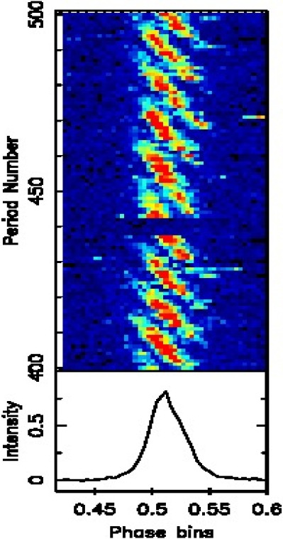
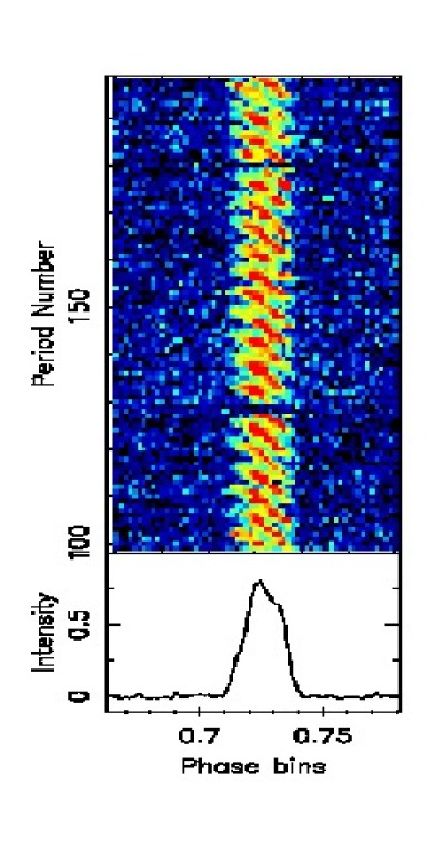
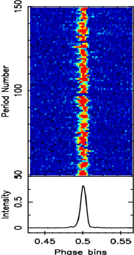
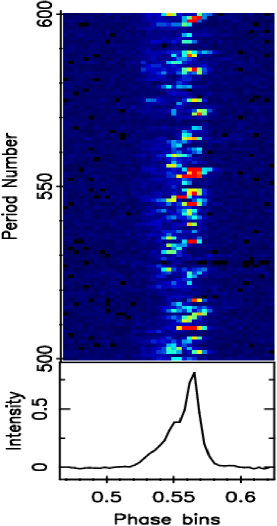
Figure 4.15.: Single pulse plot of four nulling pulsars namely PSRs (a) B0809+74 (b) B0818$-$13 (c) B0837$-$41 and (d) B2021+51 reproduced again here for a comparison. For each pulsar, 100 observed pulses are shown (see Figure 4.1 for details regarding panels).

From Figure 4.15, it can be seen that although these pulsars have similar NF of around 1%, they exhibit very different single pulse behaviour. PSRs B0809+74 and B0818$-$13 show clear drifting bands while drifting in PSRs B0835$-$41 and B2021+51 are difficult to identify from these plot. PSR B0809+74 also has very high duty cycle with much wider pulse width compared to other three pulsars. Table 4.3 lists a few basic pulsar parameters of these four pulsars for a comparison. PSR B0809+74 is among the oldest (around is 10 times) compared to the characteristic age of other three pulsars. It also shows weak inferred surface magnetic field. Although, with these differences in their derived parameters, they show similar fraction of nulling.

PSRs	Period	Age	Bsurf	$\dot{E}$
	(sec)	(years)	(G)	(ergs/s)
B0809+74	1.292241	1.22e+08	4.72e+11	3.08e+30
B0818$-$13	1.238130	9.32e+06	1.63e+12	4.38e+31
B0835$-$41	0.751624	3.36e+06	1.65e+12	3.29e+32
B2021+51	0.529197	2.74e+06	1.29e+12	8.16e+32

Table 4.3.: A few basic derived pulsar parameters Hobbs et al. (2004); Wang et al. (2001); Hobbs et al. (2004); Manchester et al. (2005) of four nulling pulsars which show similar NF of around 1%.

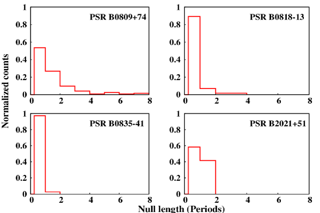
Figure 4.16.: The null length histograms of four nulling pulsars. Note the relatively larger null lengths for PSRs B0809+74 and B0818$-$13 compared to single and double period nulls in PSRs B0835$-$41 and B2021+51.

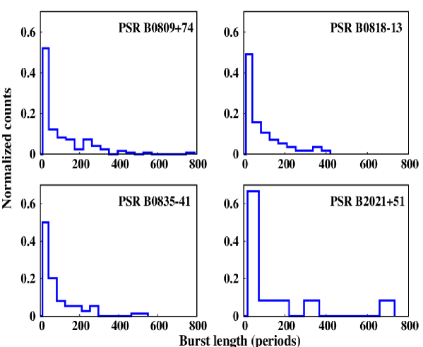
Figure 4.17.: The burst length histograms of four nulling pulsars. Note the gradual decay of burst lengths seen in all four pulsars.

To compare the nulling pattern seen in these four pulsars, we also compared their NLHs and BLHs with each other using the the Kolmogrov-smirnov test. Figure 4.16 shows the NLHs for these four pulsars. Similarly, Figure 4.17 shows the BLHs. These histograms, specially the NLHs, show significant differences between each other. PSRs B0809+74 and B0818$-$13 exhibit null lengths of around 4 to 8 periods, while PSRs B0835$-$41 and B2021+51 show only single and double period nulls. Moreover, the NLH of PSR B0835$-$41 shows around 95% of only single period nulls while less than 5% are two period nulls, which can also be seen in Figure 4.15. The NLH of PSR B2021+51 shows 60% single period nulls while the rest 40% are double period nulls. Hence, just from the visual examinations of the NLHs, it can be seen that these four pulsar have very different nulling time-scales.

4.3.2 KS-test comparison

To quantify these differences, a two sample Kolmogorov-Smirnov (KS) test Press et al. (1992) was carried out between the above mentioned four pulsars. The KS-test is a non-parametric distribution free test, applicable to unbinned data. KS-test provides a statistic, D, which is the maximum difference between the two cumulative distribution functions (CDFs). To compare the null length distributions of two pulsars, we formed their CDFs from the observed unbinned null length sequences. We found D from their CDFs and estimated the rejection probability of null hypothesis, which assumes that the measured distributions are drawn from the same underlying distribution. The results of these tests are given in Table 4.4 for each pair of the four pulsars. The null hypothesis is rejected for all pairs with high significance (except for the comparison of null lengths for PSRs B0818$-$13 and B0835$-$41, where the significance is marginally smaller). Thus, the nulling patterns differ between each of the four pulsars even though they have the same NF. This kind of differences are not only seen in pulsars with small NF, but also in pulsars with larger NF. For example, PSRs B2319+60 and B2034+19 have NF $\sim$ 30% but their NLH are different (Figures B.9 and B.7). A KS-test once again rejects the null hypothesis with high significance. Likewise, NLH for PSRs B2111+46 also differ with PSRs B2319+60 and B2034+19. However, as these pulsars have slightly different NFs, it is difficult to draw a strong conclusion from these data. Chapter 5, discusses a comparison between two pulsars namely, PSRs J1738$-$2330 and J1752+2359 with NF of around 85%, where further differences are shown with much higher significance. Hence, comparisons of null lengths at different NFs suggest that NF does not quantify nulling behaviour in full details.

	B0818$-$13(57)	B0835$-$41(74)	B2021+51(12)
B0809+74(123)	99.9 (0.48)	99.9 (0.44)	97.9 (0.52)
B0818$-$13(57)		88.5 (0.2)	98.0 (0.46)
B0835$-$41(74)			99.1 (0.48)

Table 4.4.: KS-test statistics from comparison of null length distributions between four pulsars with similar NF of 1%. The number in the parentheses beside the pulsar names are the number of null sequences used for comparison. The number given for various pairs are the significance of null hypothesis rejection, which assumes that the samples are drawn from the same distribution. The respective D values are given in the parentheses beside the rejection probabilities.

4.4 Do nulls occur randomly ?

Previous studies Herfindal & Rankin (2007b); Redman & Rankin (2009); Herfindal & Rankin (2009); Kloumann & Rankin (2010) indicated that nulling may not be random. To test the above premise, non-randomness tests were carried out on our data for 8 pulsars where it was possible to obtain the NLH and the BLH.

If the null pulses of a pulsar are characterised by an independent identically distributed (iid) random variable, for which NF represents the proportion statistics, then one can Monte-Carlo simulate synthetic data sets using a random number generator Press et al. (1992). We simulated around 10,000 random one-zero time series of the same length as that of the sequence of the observed pulses for each pulsar with a given NF. The distributions of null and burst lengths were derived from the synthetic data sets. If the underlying distribution of observed null lengths does not differ from the the simulated distribution with high significance, then it can be concluded that the observed nulls are sampled from a distribution characterising such an iid random variable, for which NF represents the proportion statistics. The above premise can be tested by carrying out a one sample KS-test Press et al. (1992). As explained in the earlier section, KS-test provides D statistic, which is the maximum deviation between the two CDFs. For our test, one CDF was obtained from a simulated null sequence while the other CDF was obtained from the observed null sequence. As usual, the test was carried out on the unbinned data. The D statistic from this comparison was averaged over all 10,000 simulated sequences.

Table 4.5 summarises significance level of rejection for the null hypothesis, which assumes that the two data sets are drawn from the same underlying distribution (or the observed nulls are drawn from a random distribution). Apart from PSRs B0818$-$13 and B2021+51 (where the significance is marginally lower - $>$ 82%), the null hypothesis is rejected at high significance for the rest of the pulsars.

A stronger test is Wald$-$Wolfowitz statistical runs$-$test Wald & Wolfowitz (1940). A dichotomous data set, such as the nulling pattern, can be represented by a series of length n consisting of n₁ 1s (i.e. burst pulses) and n₂ 0s (i.e. null pulses), with each contiguous series of 1 or 0 defined as a run, r (i.e. number of runs given in Column 9 of Table 4.2). In order to quantify the degree to which the runs are likely to represent a non-random sequence, we calculated Z, defined as,

$$Z=\frac{r-E(R)}{\sqrt{Var(R)}}.$$ (4.1)

Where, the mean of the random variable, R, is given by,

$$E(R)=1+\frac{2n_{1}n_{2}}{n_{1}+n_{2}}.$$ (4.2)

The variance of R is given by,

$$Var(R)=\frac{2n_{1}n_{2}(2n_{1}n_{2}-n_{1}-n_{2})}{(n_{1}+n_{2})^{2}(n_{1}+n_{2}-1)}.$$ (4.3)

Sampling distribution of Z asymptotically tends to a standard normal distribution in case of large n with a zero mean and unity standard deviation. Therefore, Z will be close to zero for a random sequence and the value of Z, derived from R, can be used to test the hypothesis that the given sequence is random in a distribution free manner. Note that a sequence judged random by the runs test indicates that each observation in a sequence of binary events is independent of its predecessor.

PSRs	NF(%)	KS test	Z	Runs test
B0809+74	1.42	99.9	-38.29	99.9
B0818$-$13	1.01	85.4	-10.52	99.9
B0835$-$41	1.7	99.3	-2.77	92.1
B1112+50	64	99.9	-22.37	99.9
B2021+51	1.4	82.2	-15.72	99.9
B2034+19	$\geq$26	99.9	-12.53	99.9
B2111+46	21	99.9	-17.50	99.9
B2319+60	29	99.9	-43.10	99.9

Table 4.5.: Summary of the two randomness tests, described in the text, for eight pulsars. The null hypothesis assumes that the nulls occur randomly. Rejection of the above hypothesis with the rejection significance from KS statistic and runs test statistic are given in the Column 3 and 5 respectively. NF (reproduced from Table 4.2) are given for comparison

This statistic was calculated for 8 pulsars for which the NLH and the BLH are presented in Figures B.1 to B.9 (except for PSR B1658$-$37). The results are given in Table 4.5. The observed values of Z for all 8 pulsars (except for PSR B0835$-$41) were large and hence the null hypothesis is rejected with more than 95 % significance. Even for PSR B0835$-$41, the rejection significance is 92 %, although this is not as significant as the other pulsars. Interestingly, Z is negative for all 8 pulsars suggesting that the null and burst pulses tend to occur in groups.

The preceding two tests confirm that a null (or a burst), in the null-burst sequence for the 8 pulsars studied, is not independent of the state of the pulse preceding it. In other words, individual nulls (bursts) are correlated across several periods. However, these tests place no constraint on the randomness of the duration of nulls (bursts). A careful examination of data suggests that the interval between two transition events, defined as a transition from a null to burst and vice-verse, does not depend on the duration of previous nulls or bursts and appears to be randomly distributed.

This random behaviour of the null (burst) duration is also supported by the following arguments. When the complete pulse sequence is divided into several subintervals, consisting of equal number of periods (typically 200 pulses), the count of the number of such transitions (events) is distributed as a Poisson distribution for all pulsars in our sample. Likewise, the interval between two transitions is distributed as an exponential distribution as its evident in the NLHs and BLHs shown in Appendix B. Lastly, featureless spectra are obtained from the sequence of null (burst) durations indicating no correlations between these durations. Thus, it appears that the duration of nulls and bursts can be considered as a random variable, at least over the time-scale spanned by our data for our sample of pulsars. These claims are further supported by the remarkable matching of the null length and burst length distributions with the stochastic Poisson point process presented in the next section.

In summary, the Wald$-$Wolfowitz runs tests imply non-randomness (i.e. correlation in the one-zero sequence, derived from the pulse sequence, across periods) in nulling in the sense that the absence (or presence) of emission in a given pulse is not independent of the state of the pulse preceding it, hinting a memory of the previous state. However, the duration of the null and burst states and the time instants of these transitions appear to be random. Hence, these pulsars produce nulls and bursts with unpredictable durations.

4.5 Expected time-scale for nulls and bursts

The nature of random variable, characterizing the null (burst) duration, is investigated further in this section, to also obtain the expected time-scale for nulls (bursts). The NLHs and the BLHs in Figures B.1 to B.9 suggest that the null and the burst durations are distributed as an exponential distribution, which characterizes a stochastic Poisson point process. The CDF, F(x), of a Poisson point process is given by Papoulis & Pillai (2002),

$$F(x)=1-\exp{(-x/\tau)}.$$ (4.4)

Where, $\tau$ represents a characteristic time-scale of the stochastic process. A least square fit to this simple model provides the characteristic null and burst time-scales ($\tau_{n}$ and $\tau_{b}$ respectively; equation 4.4).

Figures C.1 to C.8 show the CDFs corresponding to NLHs and BLHs for eight pulsars along with the least square fits to the proposed Poisson point process CDFs given in equation 4.4. These fits show remarkable similarity between the observed CDFs and the proposed CDF from the Poisson point process (equation 4.4). These fits suggest that the interval between one transition from null to burst state (and vice-verse) to another transition from burst to null state appears to be modelled well by a Poisson point process for these pulsars. It should be noted that, the model given in equation 4.4 need not be unique and other models may fit the CDFs equally well [See Vivekanand (1995); Wright et al. (2012); Cordes (2013)]. However, we use this model (a) as this is the simplest model suggested by our data, and (b) we did not have sufficient data to try more complicated models.

The characteristic null and burst time-scales ($\tau_{n}$ and $\tau_{b}$ respectively; equation 4.4) and the uncertainties on these parameters, obtained from these fits, are listed in Table 4.6. No fits were carried out for the CDF of nulls for PSRs B0835$-$41 and B2021+51 as only two points were available for the fit. The fitted model was checked by carrying out a two-sample KS-test in the following manner. First a pulse sequence, consisting of a million pulses, was simulated using the parameter $\tau$ obtained in these fits. Then, the NLH and the BLH were obtained for this simulated pulse sequence, which provides much larger sample of nulls and bursts than the observed sequence. A two-sample KS-test was carried out on the NLH and the BLH, obtained from the observed sequence and the simulated pulse sequence. The significance level of rejection for the null hypothesis, which assumes, in this case, that the two distributions are different, is given in Column 4 and 6 of Table 4.6 for the null and the burst durations, respectively. They are also indicated in Figures C.1 to C.8. The null hypothesis is rejected with high significance for null duration in all six pulsars, for which the fit was carried out. Apart from PSRs B2034+19 and B2319+70 the null hypothesis is rejected with high significance for the burst duration for the other six pulsars. The lower significance of rejection of null hypothesis for the burst duration in the above listed two pulsars may be due to the use of the simple model given by equation 4.4.

PSRs	Period	$\tau_{n}$	KS-prob	$\tau_{b}$	KS-prob
	(s)	(s)	%	(s)	%
B0809+74	1.29	1.9 (0.3)	99	176 (9)	98
B0818$-$13	1.24	0.7 (0.3)	99	84 (9)	78
B0835$-$41	0.75	-	-	44 (4.5)	74
B1112+50	1.66	4.8 (0.1)	99	4.3 (0.8)	88
B2021+51	0.53	-	-	21 (10)	95
B2034+19	2.07	2.6 (0.2)	99	11 (2)	22
B2111+46	1.02	1.6 (0.1)	99	8.7 (0.5)	99
B2319+60	2.26	11 (1)	94	23 (2)	33

Table 4.6.: The characteristic null ($\tau_{n}$) and burst ($\tau_{b}$) time-scale for the eight pulsars in Figures B.1 to B.9 obtained from a least squares fit to the CDF of these pulsars to a Poisson point process. These fits are shown in Figures C.1 to C.8. These time-scales have been expressed in seconds (i.e. column 3 and 5) after multiplying the fitted parameter (shown in Figures C.1 to C.8) $\tau$ in equation 4.4 with the period of the pulsar. The numbers in the parentheses are the corresponding errors on the time-scales, obtained from the least squares fits. The Kolmogorov-Smirnov probability of rejection for the null hypothesis, which assumes that the two distributions are different, are given in column 4 and 6 for the null and burst durations respectively.

4.6 Conclusions

The nulling behaviour of 15 pulsars, out of which 5 were PKSMB pulsars with no previously reported nulling behaviour, is presented in this chapter with estimates of their NFs. For four of these 15 pulsars, only an upper/lower limit was previously reported. The estimates of reduction in the pulsed emission is also presented for the first time in 11 pulsars. NF value for individual profile component is also presented for two pulsars in the sample, namely PSRs B2111+46 and B2020+28. Interesting pulse energy fluctuations around the null region is reported in PSR B1658$-$37. Possible mode changing behaviour is suggested by these observations for PSR J1725$-$4043, but this needs to be confirmed with more sensitive observations. An interesting quasi-periodic nulling behaviour for PSR J1738$-$2330 is also reported. We also reported intriguing single period core emission during the long nulls in PSR B2111+46. We find that the nulling patterns differ between PSRs B0809+74, B0818$-$13, B0835$-$41 and B2021+51, even though they have similar NF of around 1%.

The null and burst pulses in 8 pulsars in our sample appear to be grouped and seem to occur in a correlated way, when individual periods are considered. However, the interval between transitions from the null to the burst states (and vice-verse) appears to represent a Poisson point process. The typical null and burst time-scales for these pulsars have been obtained for the first time to the best of our knowledge.

4.7 Discussion

The estimates for the factor, $\eta$, by which the pulsed emission reduces during the nulls for 11 pulsars were presented for the first time in this study (Table 4.2). Although the physical process, which causes nulling, is not yet understood, it could be due to a loss of coherence in the plasma generating the radio emission or due to geometric reasons as summarized in Section 2.4. In the former case, $\eta$ provides a constraint on the process responsible for this loss of coherence. Our estimates provide lower limits for different pulsars as this estimate is limited by the available S/N. Nevertheless, reduction by two orders of magnitude is seen in at least two pulsars. If nulling is caused by a shift in the radio beam due to global changes in magnetosphere, $\eta$ provides a constraint on the low level emission and will depend on the orientation to the line-of-sight and the morphology of the beam during the null.

Our results confirm that NF probably does not capture the full detail of the nulling behaviour of a pulsar. We find that the pattern of nulling can be quite different for classical nulling pulsars with similar NFs. Estimates for typical nulling time-scales, $\tau_{n}$, for 6 pulsars in our sample were obtained for the first time. For 2 of these with a NF of about 1%, $\tau_{n}$ varies by a factor of three. In particular, the typical nulling time-scale for PSR B1112+50 (NF $\sim$ 65%) is about 2 s, more than 6 orders of magnitude less than that for the intermittent pulsar PSR B1931+24 (NF $\sim$ 75%). In the Ruderman & Sutherland (1975) model, the pulsar emission is related to relativistic pair plasma generated due to high accelerating electric potential in the polar cap. As mentioned in Section 2.4.2, changes in this relativistic plasma flow Filippenko & Radhakrishnan (1982); Lyne et al. (2010), probably caused by changes in the polar cap potential, have been proposed as the underlying cause for a cessation of emission during a null. The typical nulling time-scale, $\tau_{n}$ (and burst time-scale $\tau_{b}$) provides a characteristic duration for such a quasi-stable state, which is similar to a profile mode-change. An interesting possibility may be to relate this to the polar cap potential. In any case, any plausible model for nulling needs to account for the range of null durations for pulsars in our sample and relate it to a physical parameter and/or magnetospheric conditions in the pulsar magnetosphere.

We have extended the Wald-Wolfowitz runs test for randomness to 8 more pulsars. Results for 15 pulsars were published in previous studies Redman & Rankin (2009); Kloumann & Rankin (2010). Our sample has no overlap with the sample presented by these authors. Like these authors, we find that this test indicates that occurrence of nulling, when individual pulses are considered, is non-random or exhibits correlation across periods. Unlike these authors, all 8 pulsars in our sample show such a behaviour. This correlation groups pulses in null and burst states, which was also noted by Redman & Rankin (2009). However, the durations of the null and the burst states seem to be modelled by a stochastic Poisson point process suggesting that these transitions occur at random. Thus, the underlying physical process for nulls in the 8 pulsars studied appears to be random in nature producing nulls and bursts with unpredictable durations. More details regarding this behaviour are further discussed in Section 7.4.2.

Lastly, our estimates of NFs in Table 4.2 are consistent with those published earlier for PSRs B0809+74, B0818$-$13, B0835$-$41, B1112+50 and B2319+60 Lyne & Ashworth (1983); Biggs (1992); Ritchings (1976), which indicates that NF are consistent over a time-scale of about 30 years.

In Section 2.4, it was highlighted that nulling is an open question even after 40 years since it was first reported. Recent studies suggests that both nulling and profile mode changes probably represent a global reorganization of pulsar magnetosphere probably accompanied by changes in the spin-down rate of these pulsars Kramer et al. (2006); Lyne et al. (2010). Interestingly, such quasi-stable states of magnetosphere have recently been proposed, based on MHD calculations, to explain the release of magnetic energy implied by high energy bursts in soft-gamma ray repeaters Contopoulos et al. (1999); Contopoulos (2005); Timokhin (2010). Global changes in magnetospheric state is likely to be manifested in changes in radio emission regardless of the frequency of observations. This study motivates simultaneous multi-frequency observations of pulsars with nulling, as they will be useful to study these changes and constrain such magnetospheric models. Chapter 6 discusses similar observations conducted on two pulsars.

Chapter 5 On the long nulls of PSRs J1738$-$2330 and J1752+2359

5.1 Introduction

Nulling pulsars exhibit a variety of NFs, as shown in Table LABEL:table_all_null_psr, and one might hope that this apparently fundamental parameter could be used to characterise further aspects of the pulsar’s behaviour. However, as demonstrated in Section 4.3, our study dashed this hope and concluded that pulsars with similar low NFs ($\sim$ 1 %) are not necessarily similar in their nulling pattern. In this chapter, we set out to see if this result still holds even for pulsars with large NF ($>$ 80 %). We compare and contrast two high-NF pulsars and assess to what extent their nulling patterns follow a common statistical rule.

PSR J1752+2359 was discovered in a high Galactic latitude survey with the Arecibo telescope Foster et al. (1995). Subsequent timing observations indicated interesting single pulse behaviour with bursts up to 100 pulses, separated by nulls of about 500 pulses Lewandowski et al. (2004), giving an NF of about 80 %. This study also noted an intriguing exponential decrease in the pulse energy during a burst, a feature seen in very few nulling pulsars Rankin & Wright (2008); Bhattacharyya et al. (2010); Li et al. (2012) to the best of our knowledge. The second, PSR J1738$-$2330, as mentioned in Section 4.2, was discovered in the PKSMB survey Lorimer et al. (2006). As discussed in Section 4.2 and shown in Figures 4.10 and A.9, PSR J1738$-$2330 shows quasi-periodic bursts interspersed with long nulls at 325 MHz with a lower limit of 69% on its NF. Table 5.1 highlights some of the basic parameters for both the studied pulsars for a comparison. Note that PSR J1738$-$2330 is approximately five times slower and three times younger than PSR J1752+2359.

PSRs
	P	DM	Age	Bs
	(sec)	(pc$\cdot$cm-3)	(MYr)	($\times$1012G)
J1738$-$2330	1.98	99.3	3.6	4.16
J1752+2359	0.41	36.0	10.1	0.52

Table 5.1.: The basic parameters Lorimer et al. (2006); Lewandowski et al. (2004); Manchester et al. (2005) and the observations details for the two observed pulsars. Columns give pulsar name at 2000 epoch, period (P), dispersion measure (DM), characteristic age ($\times$10⁶ Yr) and surface magnetic field (B_s).

In previous studies of these pulsars the typical duration for single pulse observations was 1-2 hours. Such short observations, particularly for pulsars with periods around 1 s, do not yield sufficient nulls and bursts for a satisfactory comparison of their statistical properties. In this study much longer observations were undertaken to obtain a large sample of nulls and bursts in each pulsar.

The observations of both pulsars were carried out with the GMRT at 325 MHz, using the GMRT software backend (details of which are given in Chapter 3). The off-line analysis procedures are also similar to those discussed in Chapter 3 to obtain the NFs and to construct the NLHs and BLHs. For PSR J1752+2359 around 30 minutes of archival full polar data (Rankin, private communication), observed at 327 MHz from the Arecibo telescope was also analysed to confirm the presence of weak burst pulses during the null states and to compare the linear and the circular polarization profiles. Details regarding the data reduction and the polarization calibration are similar to those discussed by Rankin et al. (2013) (also see Chapter 3 for details regarding the Arecibo telescope and off-line data analysis).

The nulling patterns and their quasi-periodicities are discussed in Sections 5.2 and 5.3. The variations in the burst pulse energy and the modelling thereof is described in Section 5.4. The emission behaviour during null-to-burst transitions and vice-versa are discussed in Section 5.5. Unusual emission behaviour present in the null sequences of PSR J1752+2359 is analysed in Section 5.6. Section 5.7 discusses the polarization profiles of PSR J1752+2359. Section 5.8 examines the presence of Giant pulses in PSR J1752+2359. The results of this study and their implications are summarized in Sections 5.9 and 5.10, respectively.

5.2 Null-burst statistics

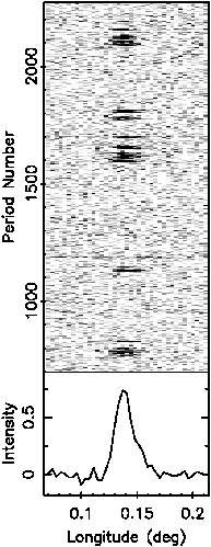
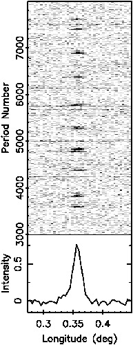
Figure 5.1.: Single pulse sequences for both pulsars in grey-scale intensities observed at 325 MHz with the GMRT. (a) A sequence of around 1500 consecutive pulses from J1738$-$2330. Short nulls, towards the end of the bright phases, can be seen for this pulsar. (b) A consecutive sequence of around 5000 pulses from J1752+2359. The quasi-periodic pattern of occurrence for bright phase is clearly evident.

Small sections of the observed single pulses are shown in Figure 5.1 for both the pulsars. Figure 5.1(a) shows around 1500 pulses for J1738$-$2330, while Figure 5.1(b) shows a section of around 5000 pulses for J1752+2359. Both the pulsars display unique nulling behaviour with a large fraction of null pulses. The arrangement of burst and null pulses in the single pulse sequence for the two pulsars showcase both similarities and differences. The single pulse sequences of Figure 5.1 show the burst pulses of both pulsars clustering together in groups, which we will refer to as the bright phases interspersed with long null phases (the inter-burst or off-phases), giving a quasi-periodic effect.

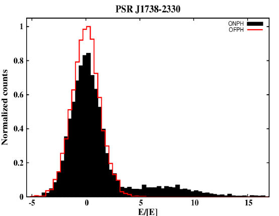
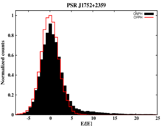
Figure 5.2.: The on-pulse (filled curve) and the off-pulse energy (red solid line) histograms for PSRs (a) J1738$-$2330 and (b) J1752+2359 obtained with the GMRT observations at 325 MHz. Both pulsars show large fraction of null pulses. J1738$-$2330 shows clear bimodal burst pulse distribution compared to smooth on-pulse intensity distribution seen for J1752+2359.

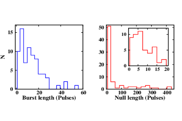
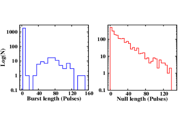
Figure 5.3.: The conventional BLHs and NLHs for PSRs J1738$-$2330  and J1752+2359 obtained from the GMRT observations. The NLH (b) for J1738$-$2330 is shown with an inset plot depicting the distributions of short nulls which is very similar to the distribution of the bursts in (a), indicating that the high NF of this pulsar arises from an excess of long nulls. The NLH (d) and the BLH (c) for J1752+2359 are shown with the measured counts on a log-scale to bring out the details for longer bursts and nulls. Note the large number of single bursts in (c), whose random occurrence among the long nulls generates an exponential distribution in the NLH (d). Thus the two pulsars have very different null distributions despite their similar NFs.

The energies in a window centred on the pulse and a window with equal number of samples away from the pulse were obtained from the single pulse sequence. The histograms for these on-pulse and off-pulse energies are shown in Figures 5.2(a) and 5.2(b) respectively for PSRs J1738$-$2330 and J1752+2359. The distributions around zero mean pulse energy in the ONPH indicate the large fraction of null pulses in both the pulsars. The NFs were estimated using the method discussed in Chapter 3 [also see Ritchings (1976)]. All the RFI affected pulses were removed during the estimation of NFs.

A NF of around 85.1$\pm$2.3% was estimated for J1738$-$2330 from the bimodal distribution in the ONPH. J1752+2359 shows large number of weak pulses and its ONPH is not bimodal. Hence, we can only estimate an upper limit of around $<$89% for the NF as some fraction of weak burst pulses will be included in the null pulse distribution. A method to separate these individual weak burst pulses from the null pulses is discussed in Section 5.6, which is similar to technique discussed in Section 3.5.4. After this separation, the fraction of null pulses are around 81% for J1752+2359. A variation up to 20 to 25 times the mean pulse energy is visible in the ONPH for both the pulsars. As both the pulsars spend about 85% of time in the null state, the estimated mean pulse energies also get reduced by the same fraction for both of them.

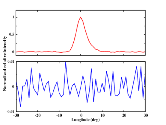
Figure 5.4.: Separated null and burst pulse profile from PSR J1738$-$2330. The top panel shows the integrated profile from all the burst pulses (solid red line), while the bottom panel shows the integrated profile from all the separated null pulses (solid blue line). Both the profiles were normalized by the peak of the burst pulse profile.

However, behind this general similarity we find a number of important differences between the two pulsars, and these can be seen in the burst and null length histograms of each pulsar (Figure 5.3). In J1738$-$2330, the lengths of the bursts [see Figure 5.3(a)] are much shorter than those typical of J1752+2359 [shown in Figure 5.3(c)] because in its bright phases, the bursts of J1738$-$2330 are equally mixed with short nulls, as can be seen from the inset of short nulls in Figure 5.3(b). Together this results in bright phases of up to 60$-$80 pulses in length, with the nulls predominating towards the end (see Section 5.4). The high NF of this pulsar then arises through the presence of a long tail of long nulls in the histogram of Figure 5.3(b). All the designated null pulses of this pulsar, whether occurring within or between bright phases, were integrated and found to show no profile of significance. Figure 5.4 shows the integrated profiles from all separated null and burst pulses for a comparison, which clearly shows absence of any emission during the nulls.

By contrast, in PSR J1752+2359 the bright phases consist of sustained non-null pulses [see Figure 5.3(c)], typically of 70-80 pulses. What is unusual about this pulsar is the very large number of isolated burst pulses which occur in the inter-burst phases. These are not evident in Figure 5.1 and can only be found by a careful inspection of the sequences. We designate them as inter-burst pulses (IBPs) and as shown in Section 5.6 that they appear at random between the bright phases, and maybe throughout the entire emission of J1752+2359. As a result, the apparently long nulls of this pulsar become subdivided in a random way giving rise to the exponential distribution strikingly visible in the NLH [in Figure 5.3(d)]. No such effect is seen in J1738$-$2330.

One consequence of the burst-null mix in the bright phases of J1738$-$2330  and the IBPs in J1752+2359 is that the conventional burst and null length histograms of both pulsars in Figure 5.3 show no evidence of the quasi-periodic behaviour of the bright and off-phases despite it being very clear in the pulse sequences shown in Figure 5.1. To overcome this, we carried out a visual inspection of the single pulses of both pulsars and identified appropriate bright phases and their separation (the separation being defined as the number of pulses between the first pulses of two consecutive bright phases).

In the case of J1738$-$2330, 21 bright phases were identified and a histogram of these is shown in Figure 5.5(a). This distribution shows a peak at around 50 to 70 pulsar periods with a spread of around 40 pulsar periods, a result which might be expected from combining the short bursts and nulls of Figures 5.3(a) and 5.3(b). Likewise, a histogram of the separations between the first pulse of two successive bright phases is shown in Figure 5.5(b). This has a surprising bimodal character with peaks around 170 and 500 pulses. Lengths of around 500 pulses cannot be formed by combining a typical burst length from Figure 5.3(a) and the longest null length from Figure 5.3(b), where the maximum is 400 pulses. We can therefore deduce that the longest inter-burst phases must be interrupted at some point by very short (and maybe weak) bursts which were rejected as burst pulses. This explains the longer off-phase stretches seen in this pulsar’s sequence of Figure 5.1 and foreshadows our discussion of this pulsar’s quasi-periodic patterns in Section 5.3. However, strong claim can not be made on the bi-modality of the bright phase separation due to their small numbers.

For J1752+2359, the identification of bright phases was a more difficult task, since it had to take into account the intrusion of IBPs in the off-pulse phases and the fact that the precise end point of a fading bright phase was sometimes difficult to fix (see Section 5.4). We were able to identify around 123 bright phases from a visual check of the single pulse sequences in the 8-hour observations. The bright phase lengths of Figure 5.5(c) show much the same distribution as the burst lengths of Figure 5.3(c) (apart from the single-pulse bursts). We find a prominent peak at around 60 pulsar periods with a spread of around 40 pulsar periods. The distributions of bright phase lengths of J1738$-$2330 and J1752+2359 are similar, but note that the former has a smaller number of bright phases. The bright phase separations of J1752+2359 also formed a broad distribution around a central peak. We measured 120 examples and the histogram is shown in Figure 5.5(d). The peak is at about 570 pulses with separations ranging from 150 to 1200 pulsar periods. The wide range of separations indicates that the nulling pattern is not strictly periodic, as can be seen in Figure 5.1, and is discussed in the next Section.

Figure 5.5.: The histograms for the length of the visually identified bright phases for PSRs (a) J1738$-$2330 (c) J1752+2359 obtained from the 325 MHz observations at the GMRT. The histograms of separation between the first pulse of successive bright phases for PSRs (b) J1738$-$2330 (d) J1752+2359 are also shown. The distributions for bright phase length are similar, while those for bright phase separation are very different

5.3 Quasi-periodicity of pulse energy modulation

In the previous section we elucidated the basic statistics of the null-burst distributions in both pulsars. Both have bright phases whose lengths are approximately normally (or possibly lognormally) distributed over lengths with a similar number of pulses [Figures 5.5(a) and 5.5(b)], but their respective separations follow very different statistics [Figures 5.5(b) and 5.5(d)]. In the case of J1738$-$2330  the separations of the bright phases have a bimodal distribution, suggesting that the pulsar must sometimes ‘skip’ a burst [Figure5.5(b)], giving an exceptionally long off-phase. In J1752+2359, the burst separations cover a very wide range from 100 up to 1000 pulses [Figure 5.5(d)]. These features are apparent in Figure 5.1, with the sequence of J1738$-$2330 including a very long off-phase, and that of J1752+2359 producing a quasi-periodic effect despite the varying separations.

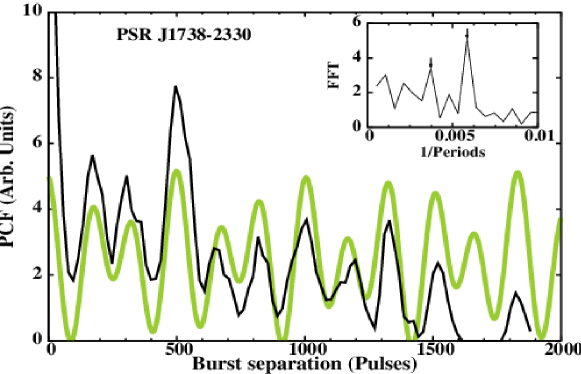
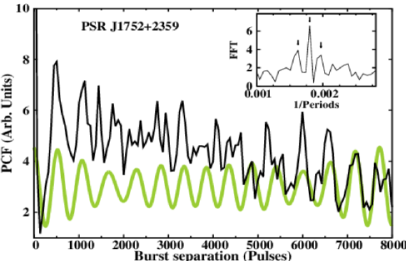
Figure 5.6.: The Pair Correlation Function for PSRs (a) J1738$-$2330 and (b) J1752+2359. The PCF is calculated as a function of measured separation between the observed burst pulses in the units of pulsar periods. The inset figures show the Fourier spectra of the corresponding PCF fluctuations (significance of these spectral features are 4$\sigma$ and 8$\sigma$ for J1738$-$2330 and 3$\sigma$, 3.5$\sigma$ and 6.5$\sigma$ for J1752+2359). The sine-waves after combining the corresponding periodicities are overlaid along with the PCFs in grey colour for comparison. Note the reduced amplitude of the PCFs for large separations due to the finite length of the observed data. PSR J1738$-$2330 shows longer quasi-periodicity coherence time-scale than that for for PSR J1752+2359. See Section 5.3 and Appendix D for more details.

To probe deeper into the nature of “quasi-periodicity” in our two pulsars, we require a suitable tool. Power spectra are a common device [as discussed in Section 4.2 for various pulsars and also by Herfindal & Rankin (2007b)], but in pulsars whose burst pulses form clusters such spectra are very much dominated by red noise due to the observed jitter in cluster separation. In the present context, a more useful procedure is to form a Pair Correlation Function (PCF) for each pulsar. This is simply a histogram of all burst-to-burst separations, whether successive or not, and can be utilized to find the coherence time over which any quasi-periodicity is maintained. A formal description of PCFs can be found in Appendix D.

The PCF for J1738$-$2330 in Figure 5.6(a) is formed from adding the burst-to-burst separation histograms from all observed pulse sequences, where each sequence is approximately 2000 pulses long. The pulse clustering is very clear and reveals a dramatic periodicity of about 170 pulses between each pulse of a cluster and the pulses in other clusters. If all bright bursts were equal in length then the height of the peaks would be equal for nearby separations and slowly decline for large separations (see Section 5.4), but we see a striking drop in the level of these peaks for the two closest bursts to a given burst, followed by a strong third peak. More distant peaks also have irregular levels, but a general periodicity of about 170 pulses is maintained. In essence, it is the structure revealed by this PCF which underlies the bimodal distribution of the burst phase separations shown in Figure 5.5(b) with its second peak at about 500 pulses.

To understand our result we formed the Fourier spectrum (FFT) of the PCF, which is shown in the inset diagram of Figure 5.6(a). This indicates two separate periodicities corresponding to approximately 170 pulses and 270 pulses, with the former dominating. The weighted sum of two sine-waves with these periodicities is overlaid on the PCF and demonstrates a good match with the PCF peaks. The 170 pulse and 270 pulse periodicities in the PCF are approximately the third and the second harmonics respectively of $\approx 500$ pulse periodicity, similar to the one obtained from Figure 4.10 in Section 4.2. The peaks produced by the dominant periodicity of 170 pulses are diminished for two successive peaks and then enhanced for the third by the weaker but significant harmonically-related periodicity of 270 pulses. The weaker periodicity is not precisely harmonically related to 170 and thereby produces a progressive difference in the peak levels. What is very remarkable is that this reproduces very closely the relative magnitude of the peaks throughout the combined 2000 pulse separation of Figure 5.6(a). This suggests an emission pattern which maintains coherence over at least 2000 pulses. However, we must caution that these results may or may not persist on time-scales longer than our observations.

The PCF for J1752+2359 [Figure 5.6(b)] has its first peak at around 500 pulsar periods. This is more pronounced than that of J1738$-$2330  but much broader in terms of pulses and it clearly corresponds to the peak found in the bright phase separations [Figure 5.5(d)]. A second peak occurs at 1150 pulses, which is little late to be simply periodic with the first peak, and later peaks show very little evidence of long-term coherence. We obtained the Fourier spectra of the PCF, which is shown in the inset diagram in Figure 5.6(b), indicating three periodic features at 540, 595 and 490 pulses, with the first dominating. The weighted sum of the three sine-waves is overlaid on the PCF but, in contrast to J1738$-$2330, the generated wave loses coherence beyond 1500 pulses as only the first two peaks are matched. Thus in J1752+2359, three sine waves are needed to yield just the two leading peaks of the PCF, in stark contrast to J1738$-$2330, where two sine waves were enough to match the entire observation. This suggests that the decomposition into sine waves has little physical significance in this pulsar.

It is indeed apparent in Figures 5.1(b) and 5.5(d) that the bursts of J1752+2359 appear with a wide variety of unpredictable separations. Thus the superficial impression of quasi-periodicity is only maintained by the fact that that the separation of successive pulses is rarely less than 500 pulses, as is indicated by the PCF. At two and three burst separations, there seems little evidence of memory operating between bursts and even less of an underlying periodicity.

5.4 Pulse energy modulation in bright phases

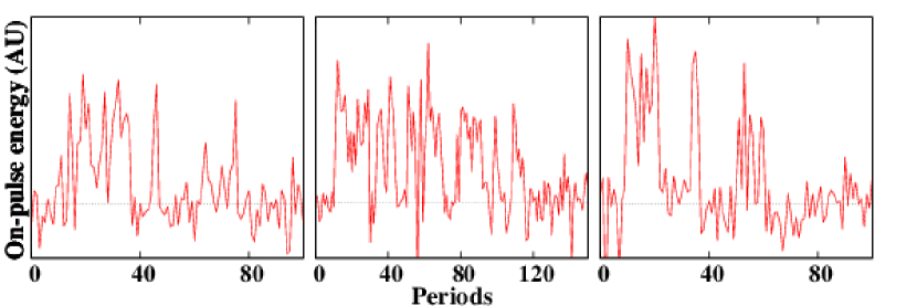
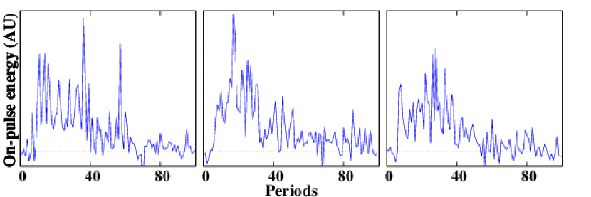
Figure 5.7.: Examples of the on-pulse energy for three bright phases for PSRs (a) J1738$-$2330 (b) J1752+2359 extracted from the GMRT observations. Both pulsars show gradual decay of the on-pulse energy at the end of the bright phase. Note the short nulls inside the bright phase for PSR J1738$-$2330. Contrary to that, most pulses of a bright phase from PSR J1752+2359 are burst pulses.

J1738$-$2330 exhibits bright phase structures of various lengths, consisting of short burst bunches interspersed with short nulls, which was also highlighted in Figure 4.9 in Section 4.2. The onset of a bright phase is relatively sudden for J1738$-$2330 with a strong burst pulse, which is followed by a change in the emission throughout the bright phase duration. This change is manifested by either a reduction in the intensity of single pulses or by an increase in the number and/or length of short null states, as can be seen in the three examples displayed in Figure 5.7(a). At the end of every bright phase, the pulsed emission clearly goes below the detection threshold and produces long null phase or off-phase. We extracted 100 pulses starting with the first identified burst pulse and averaged these over several bright phases to obtain averaged bright phase profile. A few bright phases in our observations were separated by less than 100 pulses from the next consecutive bright phase, hence they were not included in this analysis. The on-pulse energy averaged over 12 bright phases is shown in Figure 5.8(a), where a decline in the pulse intensity towards the end of the averaged bright phase is evident.

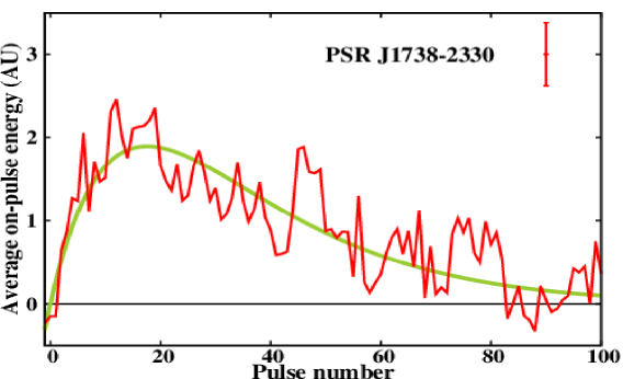
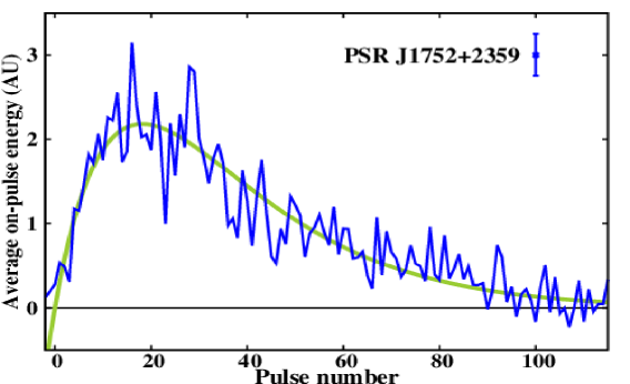
Figure 5.8.: On-pulse energy for 100 to 110 pulses, averaged over 12 bright phases, for PSRs (a) J1738$-$2330 and (b) J1752+2359 in the GMRT observations, demonstrating a similar decay in the bright phases of both pulsars. The off-pulse root-mean-square deviations are shown in the top right corner for both pulsars. The solid green lines are fitted models given by equation 5.1, with the reduced $\chi^{2}$ of around 1.2 and 1.9 for PSRs J1738$-$2330 and J1752+2359, respectively.

The onset of the bright phase in J1752+2359 is more gradual, spanning typically 5 to 10 pulses. The decline in the intensity from its peak is also more striking, as was also reported by Lewandowski et al. (2004). Figure 5.7(b) shows three examples of the decline in on-pulse energy during a bright phase in this pulsar. Note the absence of convincing null pulses during the decline. The on-pulse energy for 110 pulses, averaged from an equal number of bright phases (i.e. 12) as that for J1738$-$2330, is shown in Figure 5.8(b) to illustrate the similarity of average bright phase on-pulse energy variations in the two pulsars.

5.4.1 Bright phase modelling

Our analysis of J1752+2359 clearly shows that on-pulse energy for most of the individual bright phases follows the model given by equation 5.1. J1738$-$2330 also has a similar average on-pulse energy variation for its bright phases.

$$f(x)~{}=~{}{\alpha}\cdot{x}\cdot{e^{-(x/\tau)}}$$ (5.1)

Here, $\alpha$ is a scaling parameter and $\tau$ is the decay time-scale. The values for $\alpha$ and $\tau$ were obtained by a least-square-fit of function 5.1 to the on-pulse energy in a bright phase with errors on each energy measurement given by off pulse rms. The length of a given bright phase was defined as the difference between the two points where $f(x)$ crosses of 10% of the $f(x)_{max}$. It can be shown that $x_{max}$ is given by $\tau$. So the points where the $f(x)$ attains 10% of the peak value (i.e. $x=x_{10}$) are given by,

$${f(x)}\arrowvert{{}_{x={x_{10}}}}~{}=~{}{\alpha}\cdot{x_{10}}\cdot{e^{-(x_{10}/\tau)}}~{}=~{}{0.1}\cdot\frac{\alpha\cdot\tau}{e}.$$ (5.2)

$f(x)$ attains these values on both sides of the peak position and these points can be determined by solution of equation 5.2, obtained using numerical methods and the difference between these two points was defined as the length of a given bright phase (i.e. $L$ = $x_{10h}$ $-$ $x_{10l}$). It can be seen from equation 5.2 that values of $x_{10h}$ and $x_{10l}$ do not depend upon $\alpha$. To quantify the dependence of the bright phase length on $\tau$, we solved equation 5.2 for a range of $\tau$ values. Figure 5.9 shows the linear dependence of L on this range of $\tau$, which can also be expressed as,

Figure 5.9.: The linear dependence between the obtained 10% bright phase width (i.e. $L$) and the decay parameter (i.e. $\tau$) with a slope of $\sim$ 4.9$\pm$0.05.

$$L~{}\approx~{}4.9\times\tau.$$ (5.3)

The error on L is given by,

$$\bigtriangleup{L}~{}\approx~{}4.9\times\bigtriangleup\tau.$$ (5.4)

The average length of a bright phase derived from the above mentioned least-squares fit are 86$\pm$4 pulses and 88$\pm$3 pulses for J1738$-$2330 and J1752+2359, respectively and are consistent with the histograms of bright phase lengths discussed in Section 5.3 (Figures 5.5 and 5.5, which were obtained from the visual inspection). The length of the individual bright phase for J1752+2359 was obtained in a similar manner. Out of 123 observed bright phases in J1752+2359, only 83, with higher S/N burst pulses, were fitted to obtain their lengths (shown in Figure 5.10). We obtained the reduced $\chi^{2}$ in the range of around 0.6 to 2.2 for these fits. The average length of the bright phases from these measurements is 77$\pm$20 pulses.

Figure 5.10.: Acquired bright phase lengths obtained after the modelling 83 individual extracted bright phases for J1752+2359 with their associated errors. The bright phase lengths are shown as a function of reduced $\chi^{2}$ from the individual fit. The attained average bright phase length is around 77$\pm$20 periods from these measurements.

5.4.2 Bright phases of PSR J1752+2359

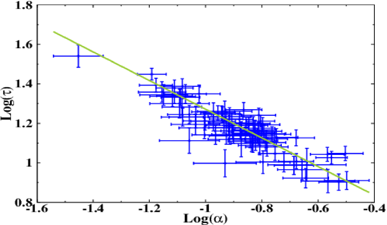
Figure 5.11.: The relationship between bright phase parameters for PSR J1752+2359 obtained from the GMRT observations. The bright phase on-pulse energy decay time-scale (i.e. $\tau$) as a function of peak of the bright phase on-pulse energy (i.e. $\alpha$) on a log-log scales. The slope was fitted after considering errors in both coordinates. A strong anti-correlation is evident in this diagram.

We could investigate the nature of bright phases in J1752+2359 further due to their large number in our $\sim$ 8 hours data, observed with the GMRT, as well as high S/N 30 minute data with the Arecibo telescope. The on-pulse energy for around 83 observed bright phases were fitted to the model given by equation 5.1 and their respective $\alpha$ and $\tau$ were obtained (shown in Figure 5.10). The log-log plot in Figure 5.11 clearly displays a power law dependence of $\tau$ with $\alpha$. The fitted line in the Figure 5.11 gives the power law index of around -0.74 $\pm$ 0.04 incorporating the errors on both axes. The Kendall$\textquoteright$s tau rank order correlation between $\tau$ and $\alpha$ is around -0.67 with a very small probability ($<10^{-7}$) of random chance. Thus, bright phases with large peak intensities decay faster for J1752+2359.

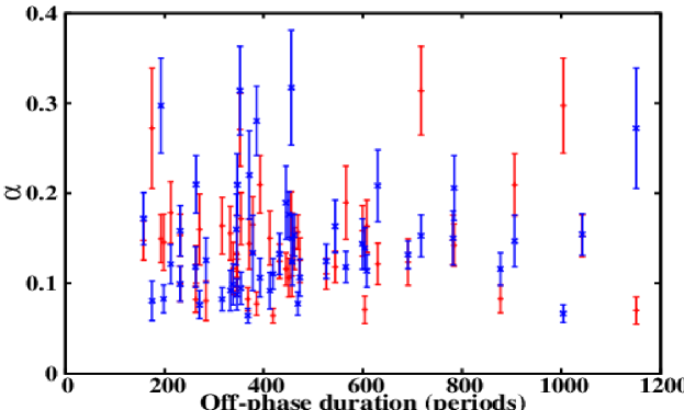
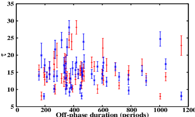
Figure 5.12.: The relationship between bright phase parameters and the off-phase durations for J1752+2359 obtained from the GMRT observations. (a) The peak of the bright phase pulse energy and (b) the decay parameter as a function of length of the associated off-phase. The red points and the blue points are parameter values of bright phases before and after the corresponding long off-phase, respectively. The scatter in the plots suggests that both the parameters are uncorrelated with the duration of off phase preceding and succeeding a given bright phase.

We also investigated the relationship between the separation between consecutive bright phases with the parameters of bright phase preceding and succeeding the null/off phase under consideration. We plotted the $\alpha$ and the $\tau$ of a bright phase as a function of the length of the off-phase preceding and succeeding it (shown in Figure 5.12). The lengths of the long off-phases were estimated as number of pulses between the last and the first pulse of two consecutive bright phases (for example number of pulses between pulse number 2885 and 3421 in Figure 5.16). We did not find any correlation as the parameters showed similar scatter for all lengths. Hence, bright phase parameters are independent of the length of the off-phase occurring before and after it.

The strong anti-correlation between $\alpha$ and $\tau$ suggests that the area under the on-pulse energy envelope for a bright phase for J1752+2359 is constant. As the full pulse energy of a bright phase can be modelled by equation 5.1, the area under a given bright phase ($A_{BP}$) was calculated by,

$$A_{BP}~{}=~{}\int_{0}^{\infty}\mathrm{\alpha}\cdot{x}\cdot{e^{-(x/\tau)}}\,\mathrm{d}x=~{}\alpha{\cdot}\tau^{2}$$ (5.5)

The error in the obtained area can be obtained after propagating the fitting error $\bigtriangleup{\alpha}$ and $\bigtriangleup{\tau}$ as,

$$\bigtriangleup{A_{BP}}~{}=~{}\bigtriangleup{\alpha}\cdot{\tau^{2}}~{}+~{}2{\alpha}\cdot{\tau}\cdot{\bigtriangleup{\tau}}.$$ (5.6)

These were calculated for the 83 observed bright phases and were the same, within errors, for all of them (shown in Figure 5.13). This indeed confirms that the total intensity of bright phase is same irrespective of its length or peak intensity and consequently, the total energy released during a bright phase is likely to be approximately constant.

Figure 5.13.: The area under the on-pulse energy modelled curve for the 83 identified bright phases with their respective errors for J1752+2359 observed from the GMRT. The distribution of the data points displays the spread of the mean is smaller compared to the errors on the individual data points, indicating the average area under every bright phase to be approximately constant.

5.5 First and Last bright phase pulse

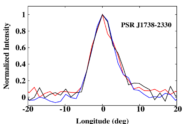
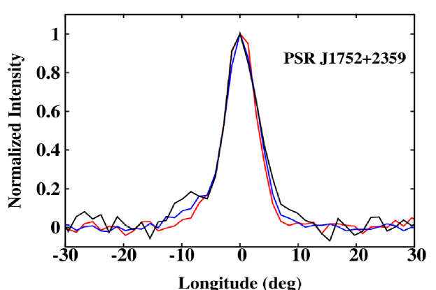
Figure 5.14.: The first-bright-phase-pulse profile (red solid line) and the last-bright-phase-pulse profile (black solid line) obtained from the GMRT observations for PSRs (a) J1738$-$2330 and (b) J1752+2359 plotted against the observed pulse phase. The blue solid lines are the average pulse profiles. All profiles were normalized with their respective peak intensities for comparison.

Compared with J1752+2359, J1738$-$2330 emits relatively strong individual pulses with high S/N during the entire span of its bright phases [as can be seen from Figure 5.7(a)]. Although the intensity of the J1738$-$2330’s pulses during a bright phase shows a decline towards its end, the energy of the last pulse is sufficiently above the detection threshold to identify them clearly. The first and the last pulse of 18 bright phases were combined to form the first-bright-phase-pulse profile and the last-bright-phase-pulse profile. Figure 5.14(a) shows these profiles for J1738$-$2330 along with its average pulse profile. All these profiles look similar. A KS-test comparison, carried out between the first-bright-phase-pulse profile and the average pulse profile, indicates similar distributions with 94% probability. Similarly, a KS-test comparison between the last-bright-phase-pulse profile and the average pulse profile also suggests similar distributions with even higher probability of 99%. These results suggest that J1738$-$2330 switches back into the bright phase mode from the off-phase (and vice-versa) without any significant change in the emission. However, these results should be treated with caution due to the small number of pulses available in forming first-bright-phase-pulse profile and last-bright-phase-pulse profile.

For J1752+2359, only 114 out of 123 observed bright phases were used to obtain the first-bright-phase-pulse as the remaining were affected by RFI. The red solid line in Figure 5.14(b) shows this profile. While the profiles look similar, a KS-test comparison between the first-bright-phase-pulse profile and the average pulse profile rejects the null hypothesis of similar distributions with 99% probability. The last pulse for most of the bright phases of J1752+2359 is very difficult to identify due to the decline in the pulse energy during this phase. Instead, a range of last pulses (10 to 20 pulses) were used for each bright phase to form the last-bright-phase-pulse profile. The length of each bright phase was determined with its associated error from the least-square-fit as explained in Section 5.4.1. To obtain the last-bright-phase-pulse profile, we averaged a range of pulses within the error bars (shown in Figure 5.10) around the expected last pulse, obtained by adding the estimated length for every bright phase to the pulse number of its first pulse. The last-bright-phase-pulse profile averaged from 114 bright phases were compared with the average pulse profile using the KS-test, which rejected the null hypotheses of similar distributions with 99.9% probability. Figure 5.14(b) shows the last-bright-phase-pulse profile with a significant ($>$ 3 times off-pulse rms) component preceding the pulse and shoulder emission after the pulse. Neither of these features is present in its average profile.

5.6 Emission in the off-phase of PSR J1752+2359

Figure 5.15.: Plot of three profiles with the normalized intensities as a function of observed pulse phase for PSR J1752+2359 obtained from the GMRT observations. (a) The pulse profile obtained from all pulses in the bright phases (9000 pulses), (b) the off-phase pulse profile from the pulses between the bright phases (41500 pulses) and (c) the absolute-null-pulse profile from the null pulses remaining after removing the IBPs (38800 pulses). All three profiles are on the similar relative scales after normalizing them with the peak intensity of the bright phase pulse profile.

In Section 5.2 we noted that, unlike J1738$-$2330, J1752+2359 exhibited intermittent single pulse bursts during the off-phase. Weak emission during an apparent null phase is not unknown Esamdin et al. (2005) and may question whether weak pulses are sometimes confused ‘true’ nulls. We therefore investigated this by forming the off-phase pulse profile by averaging all pulses between the bright phases. Those parts of the observations (about 15%), affected by the RFI, were excluded from this analysis. All the pulses in identified bright phases, amounting to around 9000 pulses, were separated from the remaining single pulse observations . The profile obtained from these pulses (i.e. bright phase pulse profile) is shown in Figure 5.15(a). The remaining 41,500 pulses, which occurred between the bright phases, were integrated to form the off-phase pulse profile. Surprisingly, the null-pulse profile showed weak emission with a significance of around 20 standard deviations [Figure 5.15(b)]. It is therefore important to clarify whether this emission originates from bright but rare single pulses and/or from underlying weak emission.

In many nulling pulsars, the burst pulses are strong enough to create a bimodal intensity distribution and can then be separated by putting a threshold between the two peaks in the histogram (as shown in Section 3.5.4). J1752+2359 does not show such a bimodal distribution due to the presence of many weak energy pulses [Figure 5.2(b)]. Hence, the use of any threshold will lead to a wrong identification of weaker burst pulses as nulls and result in a weak emission profile during the off-phase, as seen in Figure 5.15(b). This could be due to (a) weak emission throughout the off phase, (b) emission from weak burst pulses in the diminishing tail of a bright phase, or (c) emission from a few wrongly identified individual burst pulses during the off-phase.

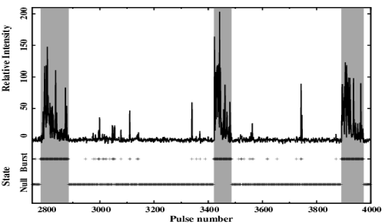
Figure 5.16.: Plot of on-pulse energy variation of around 1200 pulses of J1752+2359 observed at 327-MHz with the Arecibo telescope is shown in the top panel. The three identified bright phases are shown inside the grey shaded regions for clarity. Every individual pulse was classified either as a null or as a burst pulse. The bottom panel shows the null or burst state for the corresponding pulse consistent with a random distribution of the IBPs.

To distinguish between the above possibilities, we used higher S/N observations for this pulsar obtained from the Arecibo telescope (see Section 3.4.4 for details). Figure 5.16 shows a section of the observations from the Arecibo observation. The pulse energy plot clearly shows three bright phases with about 60 isolated single burst pulses occurring during the off-phase between them. This strongly supports our earlier suspicion that weak emission, seen during the off-phase in this pulsar, is due to these isolated burst pulses (i.e. pulses outside the bright phases or IBPs).

To investigate this further with GMRT observations, all pulses remaining after separating the bright phases were arranged in ascending order of their on-pulse energy. A variable threshold technique, discussed in Section 3.5.4, was used to separate these weak burst pulses from the null pulses. All the separated null pulses were again visually checked for wrongly identified nulls due to presence of low level RFI. The average profile, obtained from all the pulses tagged as null after this procedure, is shown in Figure 5.15(c), indicating that tagged pulses are all nulled pulses, ruling out the possibility of weak emission throughout the null.

This method of identifying the IBPs was also used on the Arecibo observation. The null or the burst state for each individual pulse was identified and is shown in Figure 5.16 in the bottom panel. It can be seen from this figure that IBPs are not localised near either the start or the end of a bright phase, but are distributed randomly inside the long off phase. In fact, these pulses may not be confined to off-phases and may occur at random through all phases since within a burst phase the their numbers would be small and not detectable. To the best of our knowledge, the presence of such pulses has not been reported in a pulsar before.

A random occurrence of IBPs implies that the rate of IBPs should remain constant. The Arecibo observation were short and hence statistical analysis of the IBP rate was not possible. Using GMRT observations we identified around 2700 such pulses, using the variable threshold method described above. As discussed in Section 5.4, the length of every bright phase was derived after fits to equation 5.1. An acceptable fit could not be obtained for a few bright phases due to either low pulse energy or due the presence of strong RFI. We only considered those off-phases bounded at both ends by bright phases, with acceptable fits. A few such off-phases were also affected by RFI and hence not included. The number of identified IBPs were counted for each off-phase and the IBP rate estimated using about 53 such off phases of various lengths. Figure 5.17 shows a histogram of the number of IBPs for a given off-phase between two consecutive bright phases. The error bars on them were obtained from Poisson statistics. Figure 5.17 clearly demonstrates that the number of IBPs are linearly correlated with the corresponding off-phase lengths. Hence, the IBP rate is independent of the length of a given null phase and could remain fixed throughout the entire emission of the pulsar.

Figure 5.17.: Plot of inter-burst pulse (IBP) counts as a function of length of off-phase between two consecutive bright phases as measured from the GMRT observations of J1752+2359. A linear relation is evident between the IBP count and the corresponding off-phase length, indicating that the IBP rate is independent of duration of off-phase.

5.7 Comparison of J1752+2359 polarization profiles

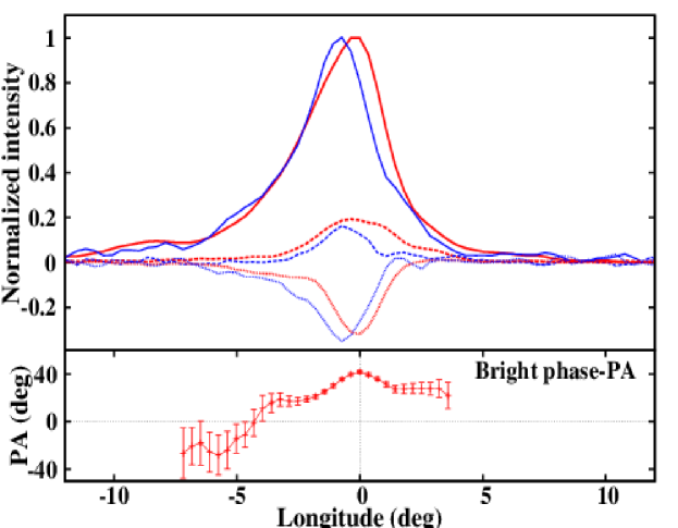
Figure 5.18.: Plot of average polarization profiles from a half-hour observation of J1752+2359 at 327-MHz using the Arecibo telescope. The total intensity profile for bright phase pulses (red solid line) and IBPs (blue solid line) are both normalised to their peak intensities. The linear polarization profiles for bright phase pulses (red dashed line) and IBPs (blue dashed line) are normalized by the peak intensity from their respective total intensity profiles. The circular polarization profiles for bright phase pulses (red dotted line) and IBPs (blue dotted line) are also normalized in a similar manner. The bottom panel shows the derived position angle (red solid line) as a function of pulse longitude for bright phase pulses. A clear offset is evident in the total intensity and the circular polarization profiles between the profiles for bright phase pulses and the IBPs.

We analysed the full polarization data from the Arecibo telescope, observed with 25-MHz bandwidth at 327 MHz (Rankin, private communication). The observed data were calibrated to measure the four Strokes parameters (i.e. I,Q,U and V). Each of the Stokes parameter was corrected for interstellar Faraday rotation, various instrumental polarization effects, and dispersion. The bright phase pulses and the IBPs were separated from the observed single pulse data and separate polarization profiles were obtained for both. The linear polarization (L) for every phase bin was measured after obtaining U and Q parameters for the corresponding phase bins by calculating $\sqrt{U^{2}+Q^{2}}$. The off-pulse mean was subtracted from it to remove the positive bias. Figure 5.18 shows the total intensity profiles along with the linear and the circular polarization profiles for the bright phase pulses and the IBPs. The position angle swing was also measured for phase bins where the observed linear polarization was more than 3 times the off-pulse RMS in the linear polarization profile. The bright phase linear polarization profile showed wider range of such phase bins. However, the IBP linear polarization profile showed very limited number of such phase bins (around 3 to 4), hence an acceptable PA swing was not possible to obtain for the IBPs. Figure 5.18 shows the PA swing for the bright phase pulses calculated by,

$$PA~{}=~{}\frac{1}{2}{tan^{-1}\bigg{(}\frac{U}{Q}\bigg{)}},$$ (5.7)

for each phase bin by the obtained U and Q profiles. The error in the PA was calculated as Mitra & Li (2004),

$$\bigtriangleup{PA}~{}=~{}\frac{\sqrt{(U\times\bigtriangleup{U})^{2}~{}+~{}(Q\times\bigtriangleup{Q})^{2}}}{2\times{L^{2}}}.$$ (5.8)

Where $\bigtriangleup{U}$ and $\bigtriangleup{Q}$ are the off$-$pulse RMS from Stokes U and Q average profiles respectively.

Figure 5.18 shows striking differences between the intensity and polarization profiles of the bright phase pulses and the IBPs. The total intensity profile of the IBPs is clearly shifted to earlier phase with respect to that of bright phase. A KS-test comparison between these two profiles rejected the null hypothesis of similar distributions with 99.9% probability. The average intensity of the IBPs is around 5 to 7 times weaker than the average bright phase pulses. A Gaussian function was fitted on both the profiles to estimate the position of their peaks. The offset between the peaks in the total intensity profiles for bright phase pulses and the IBPs was estimated to be around 0.6$\pm$0.1^∘. The linear polarization profile for the bright phase pulses is wider than that for IBPs and shows strong linear polarization of around 20% as compared to about 16% for IBPs. The shift in the position of peak intensity between these two profiles is not very significant. The circular polarization profile of the IBPs is offset from that of the bright phase pulses by 0.54$\pm$0.07^∘. However, in contrast to the overall reduction in the pulse energy during the IBPs, the IBP circular polarization fraction shows a small increase compared to that for the bright phase pulses (circular polarization of 35% and 32%, respectively) as is also evident from Figure 5.18.

5.8 No Giant pulses from PSR J1752+2359

Figure 5.19.: The on-pulse energy histogram of pulses with S/N $\geq$ 5 with the on-pulse energies scaled as explained in the text.

PSR J1752+2359 is one of the few pulsars, which showed giant pulses (GPs) at 111-MHz. The energy of these GPs was reported to be 200 times the energy of the mean pulse Ershov & Kuzmin (2005). Our data show only a gradual distribution up to 20 times the mean pulse energy [Figure 5.2(b)]. We separated all single pulses with S/N greater than 5 and estimated the mean pulse energy from these well defined burst pulses. The distribution of on-pulse energies of all burst pulses, scaled by this mean pulse energy, is shown in the Figure 5.19. indicating that these are distributed only up to 5 times the mean pulse energy, which is significantly lower than that reported by Ershov & Kuzmin (2005) at 111-MHz. In the earlier studies of GPs Staelin & Reifenstein (1968); Kinkhabwala & Thorsett (2000); Joshi et al. (2004); Karuppusamy et al. (2011), it was reported that (a) GPs have significantly smaller pulse widths compared to average pulses and (b) GPs tend to occur mostly at the edge of the average pulse profile. We separated the strongest pulses to compare their widths with that of the average pulses and no significant difference was found. While the profile for IBPs is slightly narrower and shifted towards the leading edge, their intensities are 5 to 7 times weaker than the average bright phase pulses. If the IBPs have different spectral behaviour compared to bright phase pulses, then it is likely that they may give rise to GPs at 111-MHz. However, this needs to be tested with simultaneous observations at both frequencies. Hence, it can be concluded from our data that PSR J1752+2359 does not show GPs at 325 MHz.

5.9 Conclusions

Comparison	PSR J1738$-$2330	PSR J1752+2359
NF	85.1(2.3)%	$<$ 89%
Quasi-periodicities	170 and 270 pulses	540 (490,595) pulses
Coherence of quasi-periodicities	$>$ 2000 pulses (11 peaks)	1000 pulses (2 peaks)
Variation in on-pulse energy during bright phase	Exponential decline with flickering nulls	Steady exponential decline
Length of bright phase	86 $\pm$ 4 pulses	88 $\pm$ 3 pulses
Separation between bright phases	$\sim$ 170 and 500 pulses	$\sim$ 570 pulses
Inter-burst pulses	No (?)	Yes; with a fixed random rate
First and last bright phase pulses	Similar with each other and average profile	Distinct with each other and average profile

Table 5.2.: The table of comparison between two pulsars.

As we have stressed from the start, the superficial similarity in the emission patterns of J1738$-$2330 and J1752+2359 hides many differences. J1738$-$2330 is the younger pulsar but with a stronger magnetic field, which has enabled it to spin down to a period five times longer than the older, but weaker, J1752+2359 (see Table 5.1). Nevertheless, both have arrived at a point where their nulling fractions are greater than 80% and their bursts of emission are of similar length (measured in pulses) separated by long null sequences which give the overall appearance of being quasi-periodic (Figure 5.1, Table 5.2).

However, detailed examination of the patterns of emission bursts reveals significant differences. Firstly, the burst separations of the younger pulsar J1738$-$2330 turn out to be underpinned by periodic behaviour. A histogram of the burst pulse separations (PCF in Figure 5.6) could be modelled by the superposition of two near-harmonically related sine-waves and matched to the observations for at least 2000 pulses (i.e 11 burst phases). This is strong evidence of long-term memory in this pulsar. However, although the coherence of the sine waves is not lost, individual burst phases often fail to materialise except in some vestigial form. This can be seen as the effect of the stronger sine periodicity sometimes countered by the effect of the weaker near-harmonic (2:3) periodicity.

By contrast, in J1752+2359 there is no evidence of long-term periodicity. This pulsar requires a complex wave superposition to reproduce just the first two burst phase intervals in its pulse-separation histogram (Figure 5.6b). Beyond about 1000 pulses, coherence is lost rapidly and there is no memory of any periodicity. The impression of quasi-periodicity is maintained since the burst separations usually range between 300 and 600 pulses [Figure 5.5(d)].

Additionally, J1752+2359 has a striking feature not present in the younger pulsar – and hitherto not reported in any pulsar. In the long null intervals between the bursts of J1752+2359  the nulls are interrupted at random by burst pulses which are mostly single and relatively weak in intensity (IBPs). These pulses have a profile significantly shifted with respect to the main profile and different polarisation properties (Figure 5.18), hinting at a different physical origin. They may well occur continuously through both burst and off-phases, providing a diffuse background to the pulsar’s more structured emission of bright and off-phases.

The bright phases of the pulsars, although similar in duration when measured in pulses, have different substructures. In J1738$-$2330, the bursts start suddenly and as they progress, they are increasingly punctuated by nulls until the off-phase begins [Figure 5.7(a)]. Thus the onset and the end of the bright phases are clearly marked, and profiles obtained by integrating first and last burst pulses are effectively identical to the pulsar’s overall profile [Figure 5.14(a)]. In J1752+2359, the bursts take longer to reach their peak emission, followed by an exponential decline in intensity. The bright phase fades with weak emission and it is often difficult to pinpoint its true end [Figure 5.7(b)]. There is evidence that an additional small leading component appears in the emission profile as the phase closes [Figure 5.14(b)].

In both pulsars the progression of the intensity of their burst phases can, when averaged, be fitted by the same functional form (equation 5.1, see Figure 5.8). In the case of J1752+2359, we find that individual bright phases with a higher peak intensity tend to be shorter in length with a significant anti-correlation ($-$0.7) between these two parameters (Figure 5.11), implying that the output in energy integrated over a bright phase is constant, at least at the observing frequency. Furthermore, the bright phase parameters are independent of the length of the off-phase before and after the bright phase.

5.10 Discussion

As summarized in Section 2.3.1, it has long been known that no strong correlations exist between NF and other pulsar parameters such as period or period derivative Ritchings (1976); Rankin (1986); Biggs (1992); Wang et al. (2007). This is also true here since, despite their similar NFs, the positions of PSRs J1738$-$2330 and J1752+2359 in the $P-\dot{P}$ diagram could hardly be further apart. Furthermore, Figure 5.20 clearly shows that, both are far from the so-called “death line” – contradicting a simple view that pulsars die through progressive increase in NF Ritchings (1976). However, what high NF pulsars do seem to have in common is that their individual null pulses do not appear at random with a single fixed probability. In fact, their few non-null pulses have a tendency to cluster in what we have called “bright phases”, even when these phases are separated by hours or even days Kramer et al. (2006); Li et al. (2012).

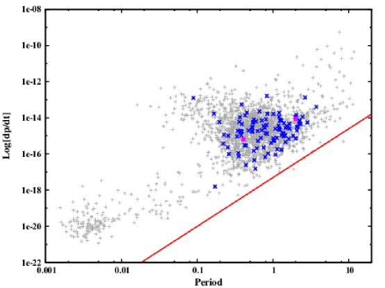
Figure 5.20.: PSRs J1738$-$2330 and J1752+2359 in the $P-\dot{P}$ diagram. All the pulsars are shown with grey points while all the known nulling pulsars (listed in Table LABEL:table_all_null_psr) are shown with blue points. Both the pulsars, studied in this chapter, are shown with magenta points. The death line, derived using the RS model is shown as red solid line (see Section 2.1.3).

The simplest way of generating clusters of bright emission is to assume a two-state probability model, such that the probability of a null during a bright phase is fixed but lower than that during an off-phase [see Section 4.5 and Cordes (2013)]. This represents an elementary Markov (Poisson point) process and results in separate exponential distributions for the null and burst lengths, so that short nulls/bursts are very common and long nulls/bursts much less likely. This model has been plausibly applied to the null and burst statistics of several pulsars with low to medium NFs [see Appendix B and C and Figure 1 of Cordes (2013)]. In all these models burst/null clustering occurs and their power spectra show broad red features, but they do not generate quasi-periodic features.

However, in the case of the two pulsars described in this chapter we have become convinced that neither of them has null/burst distributions which are exponential in form. This is most evident in the burst distribution of J1752+2359 [Figure 5.3(c)], which appears to be bimodal, and when the IBPs are disregarded [as in Figure 5.5(c)] a simple Gaussian-like distribution becomes clear. The same is true of the pulsar’s apparently exponential null distribution in Figure 5.3(d), which, on neglect of the IBPs, is transformed into a single hump in Figure 5.5(d). In J1738$-$2330, the burst/null distributions of Figures 5.3(a) and 5.3(b) are superficially exponential, but we know them to partly consist of short bursts and nulls which arise exclusively during the bright phases, again meaning that the distribution is bimodal. When these short nulls/bursts are disregarded, as in Figures 5.5(a) and 5.5(b), a single-hump distribution is evident (in fact a double hump in the case of Figure 5.5(b) for reasons given in Section 3). This line of reasoning is similar to that of Kloumann & Rankin (2010) in their study of the high NF pulsar B1944+17. They suggest that the shortest nulls of that pulsar are “pseudo-nulls”, which in fact integrate to a weak profile, leaving a hump-like distribution for the remaining nulls.

We are therefore forced to abandon the simple (Poisson point) assumption of a separate but fixed null probability for each of the two phases. Instead, we see that the probability of the length of time the two pulsars spend in their bright and off-phases is dependent on its respective Gaussian-like distribution. It is this which gives the pulse sequences their quasi-periodic character, as typical bright phase and off-phase alternate with lengths scattered around the means of their distributions.

Within this picture, the burst phases will not occur in precisely periodic sequences, but can be expected to gradually lose coherence as their separation varies randomly about a mean. This can be seen very clearly in the PCF of J1752+2359 [Figure 5.6(b)], where coherence is lost after only two peaks. In J1738$-$2330, the typical burst phase separations are less and their distribution narrower [Figure 5.5(b)], so we might expect coherence to persist for more peaks, as is indeed the case [Figure 5.6(a)]. However, the degree of coherence in this pulsar’s PCF is exceptionally high and we have been able to reproduce it well by combining just two near-harmonic underlying periodicities. This hints at the presence, at least in this pulsar, of forcing periodicities with suitable phase shifts Cordes (2013). How this is achieved physically is a matter of speculation. For example, these periodicities may arise from an external body Cordes & Shannon (2008) or neutron star oscillations Clemens & Rosen (2004) or near-chaotic switches in the magnetosphere’s non-linear system Timokhin (2010).

In both pulsars the bright phases themselves show clear evolution and therefore have some kind of internal memory (Figures 5.7 and 5.8). Both diminish in intensity and J1738$-$2330 has an increasing number of null pulses as the burst proceeds. A decline of energy during a burst has been noted in several other pulsars. Recently, Li et al. (2012) have found that PSR J1502$-$5653 has long nulls interspersed with weakening bursts (their Figure 2) whose peak drifts as the burst develops. A similar phenomenon appears to occur in PSR J1819+1305 Rankin & Wright (2008) and Bhattacharyya et al. (2010) have also reported a gradual fall in pulse intensity before the onset of null states for PSR B0818$-$41. In other studies, Young et al. (2012) report intermittent long off-phases in PSR B0823+26 and their Figure 1 clearly shows a decline in intensity before null onset. In all cases it seems that the off-phases do not come out of the blue, so that the burst phase may represent a reset or relaxation of the magnetospheric conditions. It is clear that a change-of-state occurs when the pulsars move to the off-phase, quite possibly involving a global magnetospheric change Contopoulos et al. (1999); Contopoulos (2005); Timokhin (2010).

The appearance of random isolated pulses (IBPs) during the off-phase of J1752+2359, exhibiting a different integrated profile to the burst profile, has not been reported in other long-null pulsars. Its random nature is reminiscent of RRATs and the bright single pulses which appear in the weak mode of PSR B0826$-$34 Esamdin et al. (2005) or the RRAT phase of PSR J0941$-$39 Burke-Spolaor & Bailes (2010). We cannot know if this emission represents an additional property of the stable but intermittent off-phase magnetospheric state or whether it is a permanent background phenomenon such as accretion Wright (1979), which has a separate physical origin. Recently, Young et al. (2012) also reported similar state switching between normal nulling pulsar mode and intermittent pulsar mode in PSR B0823+26.

The differences in the statistics and the structure of the bright phases of PSRs J1738$-$2330 and J1752+2359 do not necessarily imply that the two pulsars produce nulls in a fundamentally different way. It is possible that through having a stronger surface magnetic field and a wider light cylinder J1738$-$2330 is somehow able to maintain near-periodic coherence for longer than J1752+2359 (considerably longer if measured in clock time rather than pulse numbers), and possible differences in the unknown inclinations of the pulsars’ dipole axes to their rotation axes may play a role Cordes & Shannon (2008). Our results suggest that pursuing in detail the “quasi-periodic” behaviour of any pulsar may well yield valuable physical clues to the nature of its magnetosphere and environment.

An earlier study of pulsars with low NFs (Section 4.3) found that the NF percentage was not predictive of a pulsar’s subpulse behaviour. Our detailed study of PSRs J1738$-$2330 and J1752+2359 has shown that pulsars with very similar, but high, NFs can also have subtle but important differences in emission.

Chapter 6 Simultaneous multi-frequency study of pulse nulling behaviour in two pulsars

6.1 Introduction

Pulsar emission at different radio frequencies, originates at different locations in the pulsar magnetosphere Komesaroff (1970). This has been discussed with details in Section 2.2.1. All of the nulling studies, reported in Chapter 4 and 5, were carried out at a single observing frequency. Moreover, most of them were conducted only for a typical observations lasting about an hour. There are very a few long simultaneous observations of nulling pulsars reported so far in the literature. Section 2.3.4 highlights some of the studies that have been conducted to scrutinize the broadband behaviour of the nulling phenomena. Among the investigated pulsars, PSRs B0809+74 and B1133+16, represent a conal cut of pulsar beam Rankin & Ramachandran (2003); Rankin (1993), while PSR B0826$-$34 has an almost aligned pulsar beam Biggs et al. (1985). Thus, it is not clear if nulling represents a global failure of pulse radiation or is due to a shift in pulsar beam manifesting as lack of emission at the given observation frequency due to the geometry of pulse emission. Thus, as suggested in Section 2.5, long, sensitive, and preferably simultaneous observations at multiple frequencies of a carefully selected sample of pulsars are motivated by these previous investigations.

In this chapter, we report on long simultaneous multi-frequency observations of two pulsars, PSRs B0809+74 and B2319+60 to investigate the broadband nature of pulse nulling. These pulsars were chosen as (a) they are strong pulsars allowing an easy determination of nulls, (b) PSR B0809+74, show prominent drifting and single component profile [see Section 4.2 and Lyne & Ashworth (1983)] indicating a tangential and peripheral line of sight traverse of their emission beam, and (c) PSR B2319+60, show long prominent nulls and have high NF [about 30%, see Section 4.2 and Figure 4.13(c)]. It also shows a multiple component profile with drifting in outer components indicative a more central line of sight traverse of the emission beam Rankin (1986); Gould & Lyne (1998). Thus, this sample allows us to test the effect of pulse nulling as a function of observational frequency for different parts of pulsar beam and discriminate between a geometric or an intrinsic origin for pulse nulling. In Section 6.2, observations and essential time-series alignments between various observed frequencies are described. The results on PSR B0809+74 are presented in Section 6.3, while the results on PSR B2319+60 are presented in Section 6.4. The conclusions of the study are presented in Section 6.5 along with a discussion on the implications of the results in Section 6.6.

6.2 Observations and time-series alignments

Pulsar	Period	Dispersion	Date of	Number of pulses	Frequencies
		Measure	observations		of observations
	(s)	(pc cm-3)			(MHz)
PSR B0809+74	1.292241	6.12	2011 February 17	10003	313, 607, 1380, 4850
PSR B2319+60	2.256488	94.59	2011 February 6	5126	313, 607, 1380, 4850

Table 6.1.: Parameters of the observed pulsars and details of Observations

PSRs B0809+74 and B2319+60 were observed simultaneously with the Giant Meterwave Radio Telescope (GMRT), the Westerbok Synthesis Radio telescope (WSRT) and the Effelsberg Radio Telescope. The details of observations are discussed in details in Chapter 3 and also listed in Table 6.1, with exact observing frequency for a comparison.

Given the difference in the longitude of the observatories, the total overlap at all frequency was smaller than the total duration of observations at each telescope. Part of the data during the overlap was affected by radio frequency interference (RFI) at one or the other telescope and was not considered for the analysis described below. The remaining number of pulses observed simultaneously are indicated in Table 6.1.

The data from all observatories, as mentioned in Section 3.5.1.2, were converted into a standard format required for SIGPROC analysis package and dedisperesed using the programs provided in the package. These were then folded to 1000 bins across the period using polycos obtained from the ephemeris of these pulsars using TEMPO package to obtain a single pulse sequence.

First, the pulse sequence for the longest data file, typically consisting of 6000 pulses, were averaged for each frequency to obtain an integrated profile, which was used to form a noise-free template, after centering the pulse, for the pulsar at that frequency. The template at each frequency was used to estimate the number of samples to be removed from the beginning of each file for these two frequencies so that the pulse is centred in a single period and time stamps for single pulses were corrected by these offsets. The single pulse sequences were then aligned by converting these time stamps to solar system barycentre (SSB) using TEMPO². This conversion also takes into account the delay at lower frequencies due to dispersion in the inter-stellar medium (ISM). Then, the pulses corresponding to identical time stamps at SSB across all frequencies were extracted from the data. As the observations were typically recorded in 2$-$3 data files at the GMRT (325 and 610 MHz), the data recorded at the WSRT and the Effelsberg were split into similar number of files with observations duration equal to that at the GMRT.

The single pulse sequences were then visually examined to remove any single pulses with excessive Radio Frequency Interference (RFI). The number of pulses available at all frequencies simultaneously after eliminating pulses affected by RFI are indicated in Table 6.1 for each pulsar. Broadband nulling behaviour for each pulsar, using these single pulse sequences, are discussed in the following sections.

6.3 PSR B0809+74

A subset of simultaneous pulse sequences, obtained at all four frequencies, are shown in Figure 6.1. At 1380 MHz, single pulses were detected with highest S/N, while they showed relatively low S/N at 4850 MHz. The drifting of subpulses is clearly evident for single pulses at 313, 607 and 1380 MHz. To improve the single pulse S/N at 4850 MHz, we added 10 consecutive phase-bins. Thus, such drifting behaviour is not possible to identify at 4850 MHz in Figure 6.1. The simultaneity in the absence of emission is also evident across all four frequencies in Figure 6.1. Presented section of single pulses clearly shows two distinct null regions near period numbers 1640 and 1740 at each frequency. To verify and quantify this behaviour further, the NFs, the correlation between the nulling pattern represented by the one-bit sequence and the distributions of null and burst lengths were compared across four frequencies.

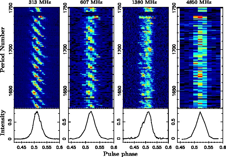
Figure 6.1.: Single pulse sequences as a function of pulse number and pulse phase for a subset of data for all frequencies for PSR B0809+74. The sequences were observed simultaneously at all frequencies. The pulse intensities are shown in a color ramp from blue to red. The bottom panel in each plot shows the respective integrated profile.

First, we obtained the on-pulse energy sequence by selecting an appropriate on-pulse window at each frequency from their respective integrated profile. Due to the interstellar scintillation, the on-pulse energy shows large fluctuations at all frequencies. As discussed in Section 1.3.3, this can cause the on-pulse energy to plunge around zero pulse energy, which makes identification of the null pulses a daunting task. Thus, for all those sections, which showed low S/N single pulses at any particular frequency (around 2% of the observed pulses), were excluded at all four frequencies. For a few different sections, pulse energy was marginally reduced which was normalized by subtracting a moving average, or a box average (see Section 1.3.3). Figure 6.2 shows sections of on-pulse energy sequences at all frequencies, after subtracting a box average. As PSR B0809+74 exhibit small fraction of null pulses separated by large burst phases, to display more simultaneous null regions, four different sections of pulse sequences around these null states were extracted for display at each frequency. The null pulses at each frequency clearly shows simultaneous occurrence across all observed frequencies. A visual inspection of the entire data broadly confirms this behaviour.

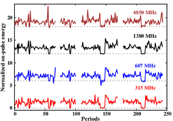
Figure 6.2.: On-pulse energy sequences as a function of pulse number for a subset of data from all four frequencies for PSR B0809+74. The ordinate present pulse energy in arbitrary units, which is presented with an offset in the vertical direction for each frequency for clarity. The dotted horizontal lines present respective zero pulse energy at a given observing frequency. The period numbers in the abscissa are superficial as four separate null regions, extracted at each frequency, are shown here to display correlated pulse energy fluctuations.

6.3.1 NFs comparison

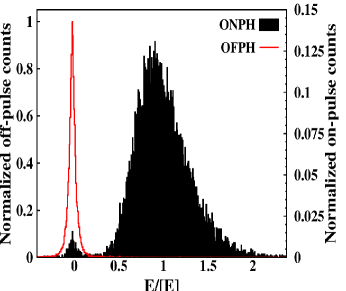
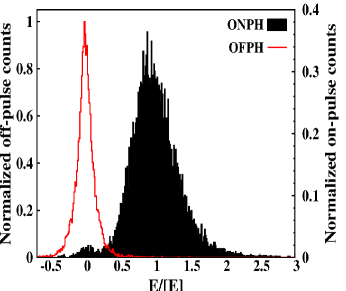
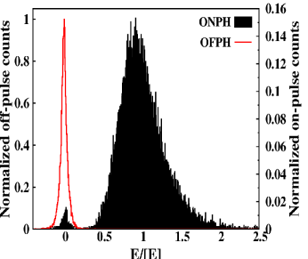
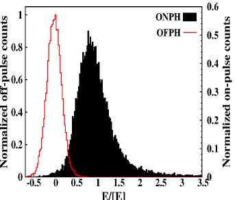
Figure 6.3.: The on-pulse and the off-pulse energy histograms at all four frequencies for PSR B0809+74, i.e. (a) 313 MHz, (b) 607 MHz, (c) 1380 MHz and (d) 4850 MHz. The abscissa presents normalized energy obtained using the block average (see Chapter 3). The ordinate presents normalized counts of occurrence for each energy bin. The OFPHs are shown with the red solid lines while the ONPHs are shown with black filled curve. The counts in both the histograms were normalized by the peak from the corresponding OFPH histogram at each frequency. The obtained NF along with the observed frequency are displayed in the inset texts. Total 10003 pulses were used to obtain these histograms at each frequency.

As a first test to quantify the similarity of nulling behaviour, obtained NFs at all four frequencies were compared. The on-pulse energy sequence and the off-pulse energy sequence at each frequency were binned. The obtained ONPHs and OFPHs are shown in Figure 6.3. All four ONPHs show very small fraction of null pulses. The method to obtain the NF is discussed with details in Section 3.5.3. The ONPHs at 313, 607 and 1380 MHz [i.e. Figure 6.3(a),(b) and (c)] show clear bi-modal distributions of the pulse energy. Thus, we were able to obtain accurate estimate of the NFs at these lower frequencies. However, at 4850 MHz the single pulse S/N was not sufficient to produce such clear bi-modal distribution in the ONPH. For such cases, consecutive pulses can be integrated to improve the S/N and to get better separation between the null and the burst pulse energy distributions in the ONPH. This technique has been used for many weak pulsars, as discussed in Chapter 4. However, PSR B0809+74 exhibit null states with significantly smaller lengths (1 or 2 periods). Integrating consecutive pulses will lead to large fraction of null pulses merging with the neighbouring burst pulses. Thus, such sub-integration was not possible to deploy for NF estimation. By using the standard Gaussian fit technique on the ONPH and OFPH (see Section 3.5.3), only an upper limit on the NF was possible to derive due to the mixture of weak burst pulses with the null pulses near the zero pulse energy. The obtained NFs are also listed in the inset text of Figure 6.3 for each frequency. Figure 6.4 shows these NFs for all frequencies, to demonstrate a good match between the obtained quantities within the error bars. Although the NF does show a good match across a decade of frequencies, as suggested in Section 4.3, it does not quantify nulling behaviour in full details. Hence, it is essential to confirm pulse-to-pulse matching of the nulling behaviour in order to check the true broadband behaviour of this phenomenon.

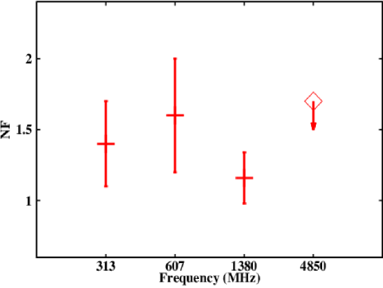
Figure 6.4.: The obtained NFs at all four observed frequencies for PSR B0809+74.

6.3.2 One-bit sequence comparison

The null pulses and the burst pulses were identified and separated at all four frequencies. For the lower three frequencies, i.e. 313, 607 and 1380 MHz, a threshold was first set on the respective ONPH, where the null pulse distribution and the burst pulse distribution overlap with each other. Pulses below the threshold were tagged as null pulses while pulses above the threshold were tagged as burst pulses. A visual inspection was carried out on the separated null and burst pulses to check for any misidentified pulses. At the highest observing frequency, 4850 MHz, single pulses were weak and hence such threshold was not possible to set to separate null and burst pulses. Hence, we initially arrange all pulses in the ascending order of their on-pulse energy. A threshold was moved from lower energy end towards the higher energy end till pulses below the threshold did not form significant profile component (with S/N$\geq$3). All the pulses below the threshold were tagged as null pulses while pulses above the threshold were tagged as burst pulses. This method, also discussed in Section 3.5.4, allows separation of weak burst pulses from true null pulses. All the separated pulses were carefully examined visually to eliminate any possibility of misidentification. Using these separated null and burst pulses, one-bit sequences were formed for all observed frequencies (see Section 3.5.6 and Figure 3.11).

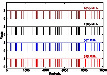
Figure 6.5.: The identified one-zero state of the pulsar emission at all four frequencies for PSR B0809+74. These pulses are not contiguous from observations. As explained in the text, different RFI affected regions as well as low S/N pulses were removed identically across all frequencies.

As a second test, one-bit sequences for a pair of observing frequencies were compared using a contingency table analysis Press et al. (1986). Figure 6.5 shows these sequences for the entire range of simultaneously observed pulses. To obtain these sequences, different observed sections were patched together at all frequencies to compare the synchronicity of null states. A visual comparison between various frequency pairs suggests that pulsar shows simultaneous switching between the null and the burst states at all frequencies, for large fraction of periods. To quantify this simultaneity, a correlation between these states for a pair of frequencies can be obtain as a 2 $\times$ 2 contingency table. In statistics, contingency table presents measure of association between two variables. In this chapter, the contingency table was used to measure the number of occurrences when the pulsar was in a similar emission state at both frequencies under consideration. Thus, such contingency table was obtained for each pair of frequencies. Table 6.2 shows the different contingency tables for all frequency pairs. It can be seen from these tables that around 9 to 11 pulses show a mismatch for different pairs of frequencies. For example, a comparison between one-bit sequences obtained at 313 and 1380 MHz indicates around 5 pulses for which the pulsar showed absence of emission at 313 MHz but it showed burst emission at 1380 MHz (see Table 6.2). Similarly, for 4 pulses, the pulsar showed absence of emission at 1380 MHz while it was in a burst state at 313 MHz. These are significantly small numbers ($<$0.1%), hence it can be concluded that PSR B0809+74 exhibit similar emission states at all pairs of frequencies for the duration of our observations.

		607
		Null	Burst
313	Null	141	4
	Burst	7	9851

		1380
		Null	Burst
313	Null	140	5
	Burst	4	9854

		4850
		Null	Burst
313	Null	140	5
	Burst	5	9853

		1380
		Null	Burst
607	Null	141	7
	Burst	3	9852

		4850
		Null	Burst
607	Null	141	7
	Burst	4	9851

		4850
		Null	Burst
1380	Null	140	4
	Burst	5	9854

Table 6.2.: Contingency tables for different pairs of frequencies for PSR B0809+74. Each frequency is shown with two corresponding emission states (i.e. the null state and the burst state). A 2 $\times$ 2 matrix for a given pair of frequencies displays number of pulses in four possible conditions.

A $\phi$ test (Cramer-V) and uncertainty test based on entropy calculations can then be used to assess the strength and significance of these correlations. Both these tests result in a value between 0 and 1. A value close to 1 indicates a strong correlation. Cramer-V for a 2 $\times$ 2 contingency table, as in our case, is just a measure of reduced chi-square. Hence, a value close to 1 indicates a very high significance of correlation. Likewise, a value close to unity for the uncertainty coefficient calculated from entropy arguments indicates a very high probability of observing null (burst) pulses at both frequencies. See Press et al. (1986) for details about these tests. The results of these tests are presented in Table 6.3. Both Cramer-V and the uncertainty coefficients have values very close to 1 for PSR B0809+74 indicating a significantly high association across all pairs of frequencies.

Frequenc	607	1380	4850
(MHz)
313	0.96	0.97	0.96
	0.92	0.92	0.91
607	$-$	0.96	0.96
	$-$	0.91	0.90
1380		$-$	0.97
		$-$	0.92

Table 6.3.: Estimate of correlation strength and significance for one-bit sequences between a pair of frequencies for PSR B0809+74. The first row in each column for a given frequency gives the Cramer$-$V indicating the strength of correlation of one-bit sequence associated with the frequency in the column. Similarly, the second row in each column for a given frequency gives the corresponding uncertainty coefficient derived from entropy arguments [See Press et al. (1986)]

6.3.3 Nonconcurrent pulses

As can be seen from Table 6.2, for a small number of pulses, the above association does not hold for various pairs. In a comparison across all four frequencies 12 pulses were found to show nonconcurrence in the emission states among 10003 compared pulses. All such pulses were carefully examined to verify their true nature and identify their locations. Surprisingly, 7 of the nonconcurrent pulses occurred either at the start or at the end of a burst. A few examples of such nonconcurrent pulses are shown in Figures 6.6, 6.7 and 6.8. As shown in Figure 6.6, at period number 415, pulsar exhibits absence of emission at 313 and 607 MHz [Figure 6.6(a) and (b)] while weak burst pulses can be seen at 1380 and 4850 MHz [Figure 6.6(c) and (d)]. As mentioned previously, a deeper examination reveals that such nonconcurrent events are most likely to occur at the transition stage. Figure 6.7 shows example of two such pulses where narrow pulsed emission can be seen at 1380 MHz, while no detectable emission is present at 313, 607 and 4850 MHz. One of these burst pulses is localized right in the middle of the long null state, while the other is located near the onset of the burst phase at 1380 MHz. On a few occasions, as shown Figure 6.8, pulsar also exhibits absence of emission at higher frequencies (i.e. 607, 1380 and 5100 MHz) while a narrow and weak burst pulse can be seen at the lowest observing frequency, 313 MHz, again near the onset of the burst phase. In summary, a comparison across all four frequencies revealed about 12 out of 10003 pulses ($\sim$0.1%) to be nonconcurrent null (or burst) state for PSR B0809+74.

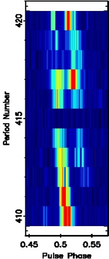
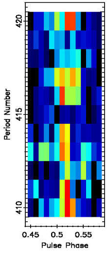
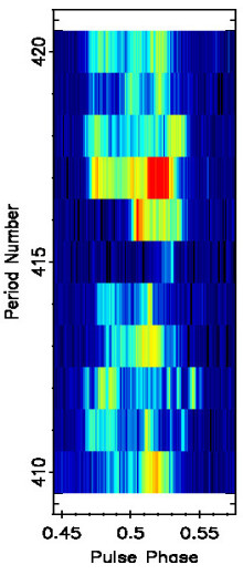
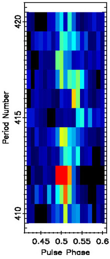
Figure 6.6.: Sections of simultaneously observed sequence of pulses at (a) 313 MHz, (b) 607 MHz, (c) 1380 MHz and (d) 4850 MHz for PSR B0809+74. At the pulse number 415, pulsar shows clear a null pulse at 313 and 607 MHz while weak burst pulses can be seen at 1380 and 4850 MHz.

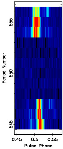
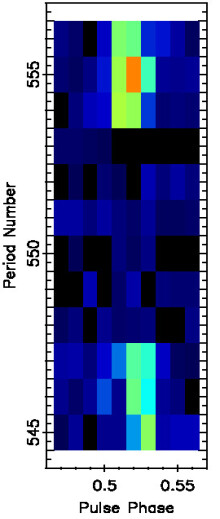
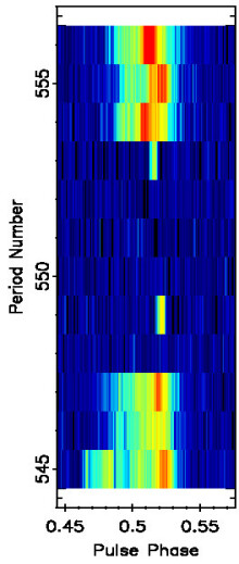
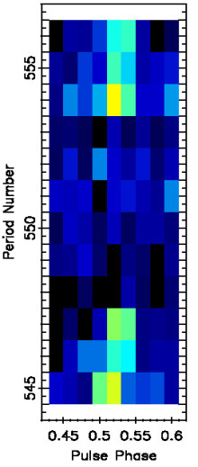
Figure 6.7.: Sections of simultaneously observed sequence of pulses at (a) 313 MHz, (b) 607 MHz, (c) 1380 MHz and (d) 4850 MHz for PSR B0809+74. At the pulse numbers 549 and 553, pulsar shows clear nulls at 313, 607 and 4850 MHz while narrow burst pulses can be seen at 1380 MHz.

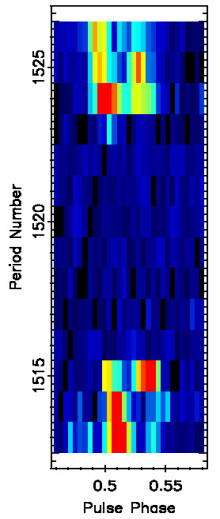
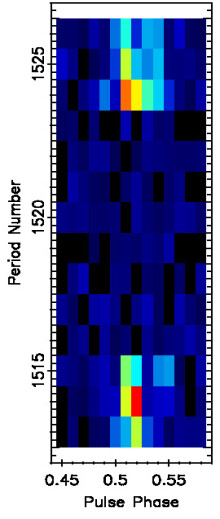
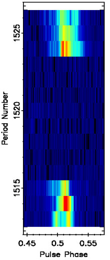
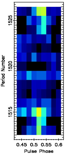
Figure 6.8.: Sections of simultaneously observed sequence of pulses at (a) 313 MHz, (b) 607 MHz, (c) 1380 MHz and (d) 4850 MHz for PSR B0809+74. At the pulse number 1523, pulsar shows clear null pulses at 607, 1380 and 4850 MHz, while a weak burst pulse can be seen at 313 MHz.

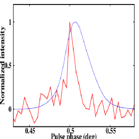
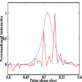
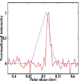
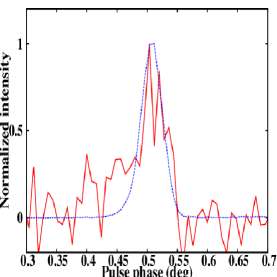
Figure 6.9.: Exclusive nonconcurrent burst pulses at (a) 313 MHz, (b) 607 MHz, (c) 1380 MHz and (d) 4850 MHz for PSR B0809+74. For each frequency, all the burst pulses (quoted in the corresponding inset texts), occuring only at a given single frequency, were averaged and shown with a red solid line. The blue dotted line represent the integrated profile at the corresponding frequency.

As its evident from Figures 6.6, 6.7 and 6.8, when pulsar displays nonconcurrence in the emission state across different frequencies, the burst emission is likely to be weak or narrow. To scrutinize this behaviour further, we identified and separated all the exclusive nonconcurrent burst pulses. These pulses were combined at each frequency and an average pulse shape was obtained, which is shown in Figure 6.9 for all frequencies. The peak S/N of these profiles are around 11, 30, 23 and 8 for the profiles at 313, 607, 1380 and 4850 MHz, respectively. For the highest observed frequency, 4850 MHz, no exclusive burst pulse was noticed. Figure 6.9(d) shows average profile from the pulses which showed emission at 4850 MHz while no detectable emission was seen at the lowest frequency (i.e. 313 MHz). Figure 6.9 also shows comparisons of exclusive nonconcurrent pulse profiles with the standard integrated profiles. The narrowness of the exclusive nonconcurrent pulse profile can be spotted easily from these figures. It should be noted that, PSR B0809+74 exhibit prominent drifting behaviour. Thus, most of the individual single pulses consist of two or three narrow subpulses. As the number of exclusive nonconcurrent pulses are very small, a broad single component smooth profile can not be obtained. This could be a likely reason behind the narrowness of the exclusive burst pulse profiles. We also can not reject the possibility of detection limits at various frequencies. If the emission is narrow and weak at a certain frequency, it is likely to be below detection limits at other frequencies. If there is an undetectable weak level emission at other frequencies, during the occurrence of exclusive burst pulse at a certain frequency, averaging these null pulses may provide a detectable component at these frequencies. However, no detectable emission was seen during the occurrence of such nonconcurrent pulses in our data. This scenario can not be truly tested here, again due to the small number of exclusive burst pulses and also due to the small number of nonconcurrent pulses for different pairs of frequencies.

6.3.4 Null length and burst length comparison

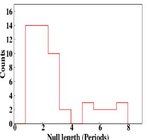
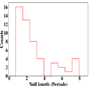
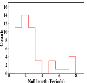
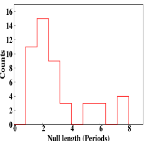
Figure 6.10.: The obtained NLHs at (a) 313 MHz, (b) 607 MHz, (c) 1380 MHz and (d) 4850 MHz for PSR B0809+74. There are minor differences near the single and double period nulls due to the small number of overall null pulses.

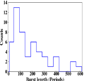
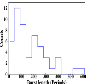
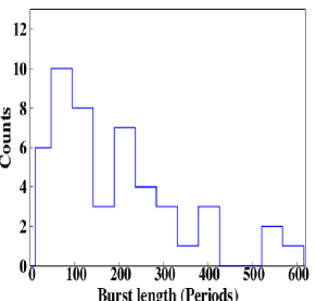
Figure 6.11.: The obtained BLHs at (a) 313 MHz, (b) 607 MHz, (c) 1380 MHz and (d) 4850 MHz for PSR B0809+74. Note the remarkable similarity between various frequencies.

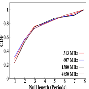
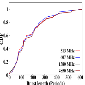
Figure 6.12.: The obtained CDFs for (a) null length and (b) burst length distributions for PSR B0809+74 at all four frequencies. Both distributions show noteworthy similarity between all observed frequencies.

Frequency	607	1380	4850
(MHz)
313	99.9	99.9	99.9
	99.9	99.9	99.9
607	$-$	99.9	99.9
	$-$	99.9	99.9
1380		99.9	99.9
		99.9	99.9

Table 6.4.: Results of a two sample KS-tests on null and burst length distributions between a pair of frequencies with the assumed null hypothesis of the two distributions being different for PSR B0809+74. The first row in each column for a given frequency gives the probability of the two distributions being similar for the null length and the second row gives that for the burst length.

To check the effect of small number of nonconcurrent emission states, on the overall nulling pattern at various frequencies, their NLHs and BLHs were compared. As elaborated in Section 6.3.3, more then half of the nonconcurrent pulses are localized either at the start or at the end of the burst phase. This can be further tested by comparing overall null length and burst length distributions, which should not show significant differences. The separated null and burst pulses, as discussed in Section 6.3.2, were used to construct the NLHs and the BLHs for all observed frequencies (Figures 6.10 and 6.11). Figure 6.10 shows the similarity in the null length distribution across all observed frequencies. The minor differences seen at the single and double period nulls occur due to the a few nonconcurrent pulses. These differences are superficial and only due to the small number of overall null pulses seen in this pulsar. To check the statistical significance of the similarity between the null length distributions, we carried out a two sample KS-test, assuming a null hypothesis of different distribution. Figure 6.12(a) shows CDFs, obtained using the observed null lengths, for all four frequencies which presents analogous distributions. Similarly, Figure 6.11 shows almost identical burst length distributions. To quantify these similarities, these distributions were again compared using the two sample KS-test, assuming a null hypothesis of different distribution. Figure 6.12(b) again shows the remarkable similarity between CDFs, obtained using the observed burst lengths at all four frequencies. Table 6.4 summarizes the results on both comparisons for each pair of observing frequencies. For all pairs of frequencies, the null hypothesis was rejected, at a very high significance, confirming the alternate hypothesis that these distributions for a pair of frequencies are similar. This confirms that nonconcurrent pulses occur near the null to burst transitions (or vice-verse).

Thus, while the nulling patterns for this pulsar is largely broadband, deviations from this behaviour is seen in about 0.1 percent of pulses, more than half of which occur at the transition from null to burst (or vice-verse).

6.4 PSR B2319+60

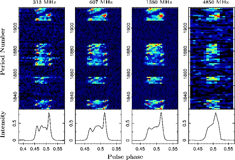
Figure 6.13.: Single pulse sequence as a function of pulse number and pulse phase for a subset of data for all frequencies for PSR B2319+64. The sequences were observed simultaneously at all frequencies. The bottom panel in all four plots displays respective integrated profile for the corresponding frequency.

PSR B2319+60, as also discussed in Section 4.2, is a strong mode-changing pulsar with a prominent drifting in the outer two conal components. This section discusses the broadband behaviour of the nulling phenomenon seen in this pulsar. Sections of observed single pulse sequences are shown in Figure 6.13 at all four observed frequencies. A clear drifting feature in the conal component can be seen at 313, 607 and 1380 MHz. For the highest observed frequency, to improve the single pulse S/N, consecutive phase-bins were added, to give a total of 125 bins across the profile. Thus, such drifting behaviour is not possible to spot in Figure 6.13. Moreover, Figure 6.13 clearly shows three distinct null states between period numbers 1837–1851, 1859–1867 and 1887–1905. The simultaneity in the absence of emission is also evident across all four frequencies in Figure 6.13. To scrutinize and quantify this behaviour further, the NFs, the correlation between the nulling pattern represented by the one-bit sequence and the distributions of null and burst lengths were compared across four frequencies.

Similar to PSR B0809+74, we obtained the on-pulse energy sequence by selecting an appropriate on-pulse window at each frequency from their respective integrated profile. Figure 6.14 shows sections of concurrent on-pulse energy sequences at all four frequencies. The coordinated pulse energy fluctuations are also evident from these time-series. The on-pulse energy clearly plunges to zero level for around six times, depicting an occurrence of null state at each frequency. These null states clearly show simultaneous occurrence across all observed frequencies. A visual inspection of the entire data broadly confirms this behaviour.

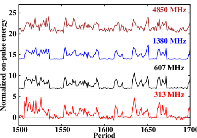
Figure 6.14.: On-pulse energy sequences as a function of pulse number for a subset of data at all four frequencies for PSR B2319+60. The ordinate present pulse energy in arbitrary units, which is presented with an offset in the vertical direction for each frequency for clarity. The dotted horizontal line presents respective zero pulse energy at a given observing frequency. The abscissa presents the sequence of contiguous period numbers. The simultaneous pulse energy fluctuations is clearly evident across all four frequencies.

6.4.1 NF comparison

A few sections of the data, specially at the lower frequencies, showed presence of RFI. These sections were removed at each frequency before estimating corresponding NFs. The obtained NFs at all four frequencies were compared as the first test to quantify the similarity of nulling behaviour. Figure 6.15 shows the obtained ONPHs and OFPHs for all observed frequencies. Each ONPH, at the corresponding observed frequency, point towards a significant number of null pulses, presented as a separate distribution around the zero mean pulse energy. The method to obtain the NF is discussed with details in Section 3.5.3. The number of pulses used during these estimation are indicated in the inset texts at the respective frequency plots. The ONPHs, obtained from the single pulses, at 313, 607 and 1380 MHz [i.e. Figure 6.15(a),(b) and (c)] show clear bi-modal distributions of the pulse energy. Thus, we were able to obtain accurate estimate of the NFs at these lower frequencies. However, at 4850 MHz, as previously mentioned, the single pulse S/N was not sufficient to produce such clear bi-modal distribution in the ONPH. Hence, 3 consecutive pulses were integrated to obtain the ONPH and OFPH. Such integration, as discussed in Section 3.5.3, will lead to a lower estimate of the NF as few null pulses will get mixed with the neighbouring burst pulses. Figure 6.15(d) shows a lower limit on the NF at 4850 MHz due to the sub-integrations. The obtained NF is also listed in the inset texts of Figure 6.15 for each frequency. Figure 6.15 demonstrate a good match between the obtained NFs within the error bars. Although the NF does show a good match across a decade of frequencies, as suggested in Section 4.3, it does not quantify nulling behaviour in full detail. Hence, it is essential to confirm pulse-to-pulse matching of the nulling behaviour in order to check if this phenomenon is truly broadband.

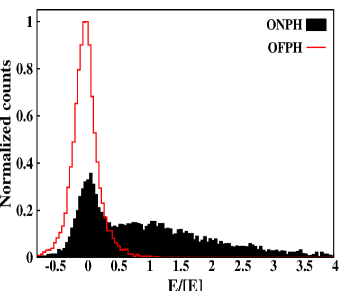
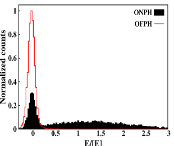
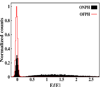
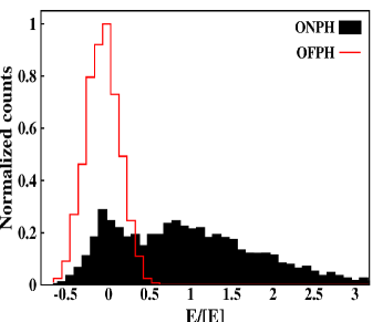
Figure 6.15.: The on-pulse and the off-pulse energy histograms at (a) 313 MHz, (b) 607 MHz, (c) 1380 MHz and (d) 4850 MHz for PSR B2319+60. The abscissa presents normalized energy obtained using the block average (see Section 3.5.3). The ordinate presents normalized count of occurrences for each energy bin. The OFPHs are shown with the red solid lines while the ONPHs are shown with black filled curves. The counts in both the histograms were normalized by the peak from the corresponding OFPH histogram at each frequency. The observed frequency, the NF and the number of pulses used during the analysis are displayed in the inset texts.

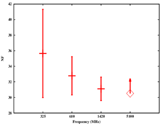
Figure 6.16.: The obtained NFs at all four observed frequencies for PSR B2319+60.

6.4.2 One-bit sequence comparison

The null pulses and the burst pulses were identified and separated at all four frequencies. For the lower three frequencies, i.e. 313, 607 and 1380 MHz, a threshold was first set on the respective ONPH, where the null pulse distribution and the burst pulse distribution overlapped each other. Pulses below the threshold were tagged null pulses while pulses above the threshold were tagged as burst pulses. A visual inspection was carried out on the separated null and burst pulses to separate any misidentified pulses. At the highest observing frequency, 4850 MHz, single pulses were weak and hence such threshold was not possible to set to separate null and burst pulses. We first obtain the single pulse ONPH and OFPH which showed large fraction of null pulses due to the mixture of true null pulses with the weak burst pulses near the zero pulse energy. A slightly higher threshold was first set in such a way that it included all null pulses below it. Pulses above this higher threshold were all high S/N burst pulses, while pulse below the threshold presented a mixture. Pulses, only belonging to this mixture, were arranged in the ascending order of their on-pulse energy. A threshold was moved from the lower energy end towards the higher energy end till pulses below the threshold did not form a significant profile component (with S/N$\geq$3). All the pulses below the threshold were tagged as true null pulses while pulses above the threshold were tagged as burst pulses (see Section 3.5.4). All the separated pulses were carefully examined visually to eliminate any possibility of misidentification. Using these separated null and burst pulses, one-bit sequences were formed at all observed frequencies, in which zero represents a null and one represents a burst. Figure 6.17 shows a section of around 350 pulses with their identified emission states at all frequencies.

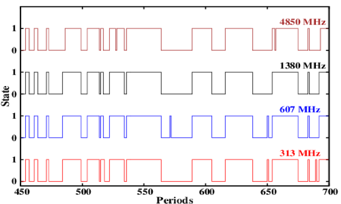
Figure 6.17.: The identified one-zero states of the pulsar emission at all four frequencies for PSR B2319+60.

The one-bit sequences for a pair of observing frequencies were compared using a contingency table analysis Press et al. (1986), as a second test. A visual comparison between various frequencies clearly confirms that pulsar shows simultaneous switching between the null and the burst states at all frequencies. To quantify this simultaneity, the correlation between these states for a pair of frequencies can be obtain, as a 2 $\times$ 2 contingency table (see Press et al. (1986) and section 6.3.2 for details). Table 6.5 shows these different contingency tables for all frequency pairs. It can be seen from these tables that around 14 to 77 pulses show a mismatch between different pairs of frequencies. For example, a comparison of one-bit sequence between 313 and 1380 MHz shows around 21 pulses for which the pulsar showed absence of emission at 313 MHz but it showed burst emission at 1380 MHz (see Table 6.2). Similarly, for 14 pulses, the pulsar showed absence of emission at 1380 MHz while it was in a burst state at 313 MHz. Total number of pulses which were compared for each pair were around 5126 pulse, hence these numbers presents a small fraction of nonconcurrence. Hence, it appears that PSR B2319+60 exhibits similar emission states at all pairs of frequencies for the duration of our observations.

		607
		Null	Burst
313	Null	1524	39
	Burst	14	3532

		1380
		Null	Burst
313	Null	1545	21
	Burst	14	3522

		4850
		Null	Burst
313	Null	1492	60
	Burst	70	3461

		1380
		Null	Burst
607	Null	1526	14
	Burst	21	3544

		4850
		Null	Burst
607	Null	1485	42
	Burst	77	3484

		4850
		Null	Burst
1380	Null	1508	37
	Burst	65	3487

Table 6.5.: Contingency tables for different pairs of frequency for PSR B2319+60. Each frequency is shown with two corresponding emission states (i.e. the null state and the burst state). A 2 $\times$ 2 matrix for a given pair of frequencies displays number of pulses in four possible conditions. It should be noted that total number of pulses are not similar for different pairs as a few weak pulses were further avoided, only for certain frequency pairs, where a decision regarding their true emission state was not possible to make.

A $\phi$ test (Cramer-V) and uncertainty test based on entropy calculations can then be used to assess the strength and significance of these correlations. These tests are briefly discussed in Section 6.3.2. See Press et al. (1986) for details about these tests. The results of these tests are presented in Table 6.6. Both Cramer-V and the uncertainty coefficients have values very close to 1, indicating a significantly high association across all pairs of frequencies. However, the strength is marginally smaller for association between pairs involving 4850 MHz.

Frequenc	607	1380	4850
(MHz)
313	0.98	0.98	0.94
	0.91	0.93	0.81
607	$-$	0.98	0.94
	$-$	0.94	0.83
1380		$-$	0.95
		$-$	0.85

Table 6.6.: Estimate of correlation strength and significance for one-bit sequences between a pair of frequencies for PSR B2319+60. The first row in each column for a given frequency gives the Cramer$-$V indicating the strength of correlation of one-bit sequence associated with the frequency in the column. Similarly, the second row in each column for a given frequency gives the corresponding uncertainty coefficient derived from the entropy arguments (See Press et al. (1986))

6.4.3 Nonconcurrent pulses

As can be seen from Table 6.5, for a small number of pulses, the above association does not hold. In a comparison across all four frequencies, about 158 out of 5126 pulses ($\sim$ 3%) do not show concurrent null (or burst) state for PSR B2319+60. All such pulses were carefully examined to verify their true nature and identify their locations. Surprisingly, 82 of these nonconcurrent pulses ($\sim$52% nonconcurrent pulses) occurred either at the start or at the end of a burst. A few examples of such nonconcurrent pulses are shown in Figures 6.18, 6.19 and 6.20. As shown in Figure 6.18, pulsar showed absence of emission at 313 and 607 MHz [Figure 6.18(a) and (b)] while weak and narrow burst pulses can be seen at 1380 and 4850 MHz [Figure 6.18(c) and (d)]. Figure 6.19 shows example of a pulse that is seen to produce detectable emission at 313, 607 and 1380 MHz, [Figures 6.19(a),(b) and (c)] while no detectable emission is present at 4850 MHz. Similarly, during a burst to null transition, as shown in Figure 6.20, a narrow weak pulse can be seen at 1380 MHz [Figure 6.20(c)] while no detectable emission is present at 313, 607 and 4850 MHz [Figure 6.20(a), (b) and (d)].

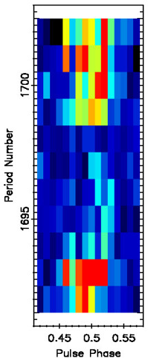
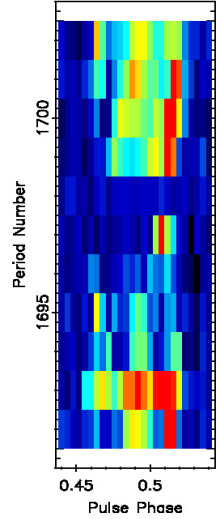
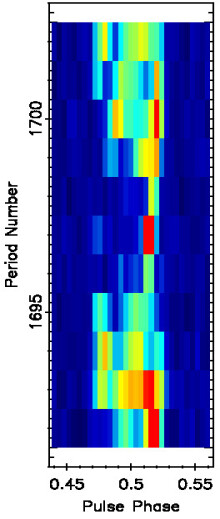
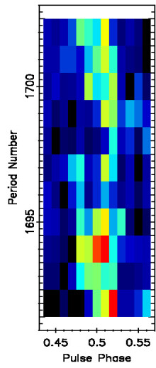
Figure 6.18.: Sections of simultaneously observed sequence of pulses at (a) 313 MHz, (b) 607 MHz, (c) 1380 MHz and (d) 4850 MHz for PSR B2319+60. At the pulse number 1698, pulsar shows clear null pulses at 313 and 607 MHz while narrow burst pulses can be seen at 1380 and 4850 MHz.

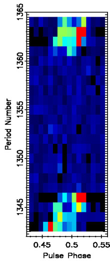
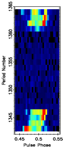
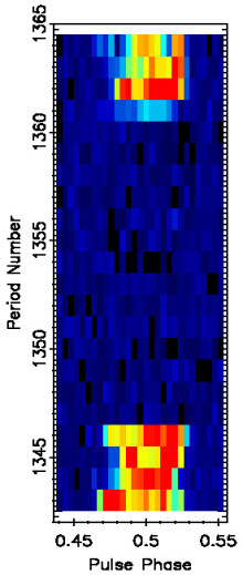
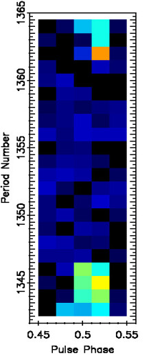
Figure 6.19.: Sections of simultaneously observed sequence of pulses at (a) 313 MHz, (b) 607 MHz, (c) 1380 MHz and (d) 4850 MHz for PSR B2319+60. At the pulse number 1361, pulsar shows clear null pulse at 4850 MHz, while weak burst pulses can be seen 313, 607 and 1380 MHz. However, such descripencies are likely to come from low S/N at 4850 MHz.

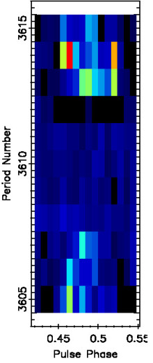
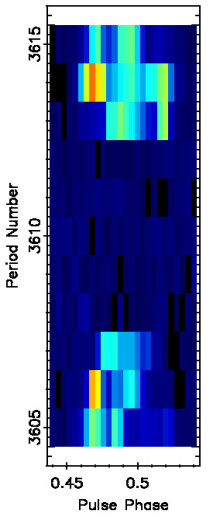
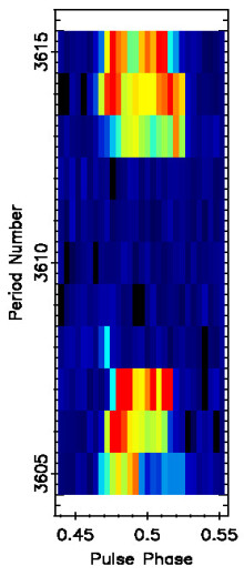
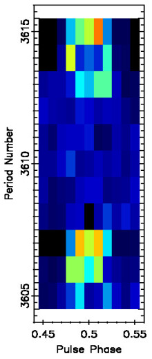
Figure 6.20.: Sections of simultaneously observed sequence of pulses at (a) 313 MHz, (b) 607 MHz, (c) 1380 MHz and (d) 4850 MHz for PSR B2319+60. At the pulse number 3608, pulsar shows clear null pulses at 313, 607 and 4850 MHz while a narrow burst pulse can be seen at 1380 MHz.

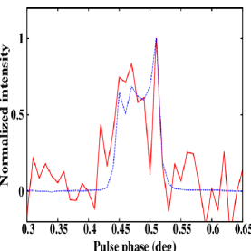
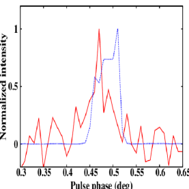
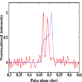
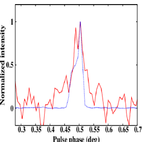
Figure 6.21.: Exclusive nonconcurrent burst pulses at (a) 313 MHz, (b) 607 MHz, (c) 1380 MHz and (d) 4850 MHz for PSR B2319+60. For each frequency, all the burst pulses (quoted in the corresponding inset texts), occuring only at a given single frequency, were combined and the average profile is shown with a red solid line. The blue dotted line represents the integrated profile at the corresponding frequency.

As it is evident from Figures 6.18, 6.19 and 6.20, when pulsar displays nonconcurrence in the emission state across different frequencies, the burst emission is likely to be weak (also narrow on a few occasions). To scrutinize this behaviour further, we identified and separated, all the exclusive nonconcurrent burst pulses (similar to those mentioned in Section 6.3.3 for PSR B0809+74). These pulses were combined and the average profile was obtained at each frequency. These profiles are shown in Figure 6.21 from the exclusive pulses at all frequencies. Approximately 7 to 13 pulses were averaged to obtain these profiles. It should be noted that these pulses are only seen to occur at a given observed frequency while they show absence of emission at all other frequencies. Thus, they are smaller in numbers compared to number of pulses given in Table 6.5 for different pairs. The peak S/N of these profiles are relatively low (i.e. peak S/N of 4.6, 7, 15 and 7.5 at 313, 607, 1380 and 4850 MHz respectively) compared to PSR B0809+74.

6.4.4 Null length and burst length comparison

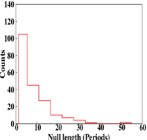
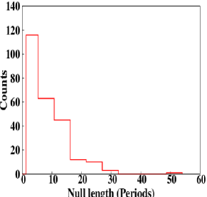
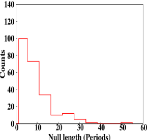
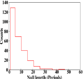
Figure 6.22.: The obtained NLHs at (a) 313 MHz, (b) 607 MHz, (c) 1380 MHz and (d) 4850 MHz for PSR B2319+60. There are minor differences near the single and double period nulls due to the small number of overall null pulses.

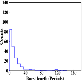
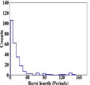
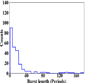
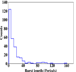
Figure 6.23.: The obtained BLHs at (a) 313 MHz, (b) 607 MHz, (c) 1380 MHz and (d) 4850 MHz for PSR B2319+60. Note the remarkable similarity in the burst length distribution across all observed frequencies.

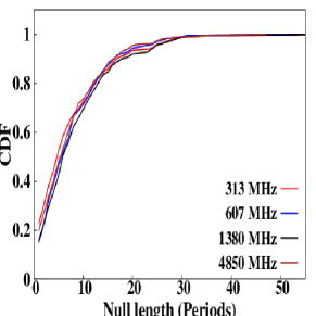
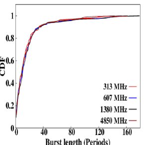
Figure 6.24.: The obtained CDFs of (a) null length and (b) burst length distributions for PSR B2319+60 at all four frequencies. Both distributions show noteworthy similarity between all observed frequencies.

Frequency	607	1380	4850
(MHz)
313	99.9	99.7	99.9
	99.9	99.9	99.9
607	$-$	99.9	99.9
	$-$	99.9	99.9
1380		99.9	99.9
		99.9	99.7

Table 6.7.: Results of a two sample KS-tests on null and burst length distributions between a pair of frequencies with the assumed null hypothesis of the two distributions being different for PSR B2319+60. The first row in each column for a given frequency gives the probability of the two distributions being similar for the null length and the second row gives that for the burst length.

Similar to PSR B0809+74, to check the effect of nonconcurrent emission states on the overall nulling pattern at various frequencies, their NLHs and BLHs were compared. As elaborated in Section 6.4.3, more than half of the nonconcurrent pulses are localized either at the start or at the end of the burst phase. This can further be tested by comparing the overall null length and burst length distributions, which should not show significant differences. The separated null and burst pulses, as discussed in Section 6.4.2, were used to obtain the NLHs and the BLHs for all observed frequencies (they are shown in Figures 6.22 and 6.23). Figure 6.22 shows the NLHs with similar exponential decay in the null length distributions across all observed frequencies. A two sample KS-test, assuming a null hypothesis of different distribution was carried out between these distributions. Figure 6.24(a) shows CDFs, obtained using the observed null lengths, at all four frequencies which presents remarkably similar distributions. Table 6.7 shows a high significance ($>$99%) in rejecting the null hypothesis for all pairs of frequencies, confirming similar null length distributions at all frequencies. Similarly, Figure 6.23 also shows almost identical burst length distributions. Figure 6.24(b) again shows the remarkable similarity between the CDFs obtained using the observed burst lengths at all four frequencies. Table 6.7 summarizes results on a comparison of the burst length distribution, using a two sample KS-test conducted for each pair of frequencies. Here also the null hypothesis, which assumed different burst length distributions, was rejected with a very high significance ($>$99%), confirming the alternate hypothesis that these distributions for each pair of frequencies are similar. This ascertain our results on the location of the nonconcurrent pulses, as they do not change the overall length distributions. Thus, while the nulling patterns for this pulsar is largely broadband, deviations from this behaviour is seen in about 3% of pulses, more than half of which occur at the transition from null to burst (or vice-verse).

6.5 Conclusion

A detail study on the simultaneous occurrence of the nulling phenomena in two pulsars, PSRs B0809+74 and B2319+60, is being reported in this chapter. The observations were conducted simultaneously at four different frequencies, 313, 607, 1380 and 4850 MHz, from three different telescope including the GMRT, the WSRT and the Effelsberg. The overlap time for each pulsar was around 6 hours between different observatories.

We obtain single pulses at each frequency and the on-pulse energies were compared across all four frequencies, which showed remarkable similarity in the pulse energy fluctuations (Figures 6.2 and 6.17) for both the pulsars. To quantify these similarities, we obtain the NF at each frequency which showed a clear matching, within the error bars, at all four frequencies for both the pulsars (Figures 6.4 and 6.16). Similarly, the one-bit sequences were also compared using the contingency table analysis. The significance of association across frequencies was measured using the Cramer-V and the uncertainty coefficient. For PSR B0809+74, both the statistical tests showed highly significant concurrent behaviour. For PSR B2319+60, the significance was marginally lower for the pairs involving 4850 MHz.

We also scrutinize all the nonconcurrent pulses for both the pulsar to investigate their true nature. For PSR B0809+74, we found that out of 12 nonconcurrent pulses, 7 (about 58%) occurred at the transition point where emission state is switching from null to burst (or vice-verse). Similarly for PSR B2319+60, we found that out of 158 nonconcurrent pulses, 82 (about 52%) occurred at the transition point where emission state is switching. Thus, both pulsars showed remarkable similarity in the overall broadband behaviour, also accounting the fraction of nonconcurrent pulses at the transition points. All exclusive pulses were separated and their aggregate power was obtained. It can be concluded from these exclusive pulses that, during a nonconcurrence event, pulsar exhibit weak and narrow emission. Thus, it is likely that these pulses occur due to different detection limits at various frequencies. A slight difference can be seen for the exclusive pulse profiles between both the pulsars. PSR B0809+74 showed significantly narrow pulses (except at 4850 MHz) aligning the overall pulse profile, while PSR B2319+60 showed significantly weak pulses shifted towards the leading edge compared to the overall pulse profile. However, a strong claim can not be made regarding their true shapes, due to their small numbers (inset texts of Figures 6.9 and 6.21). Moreover, both the pulsars exhibit prominent drifting behaviour which could easily give rise to such differences for individual pulses. Thus, shape of the exclusive profiles should be interpreted carefully. We also compared the null length and the burst length distributions across all observed frequencies which showed similar distribution with high significance ($>$99%) for both the pulsars.

6.6 Discussion

We find that nulling is broadband for PSRs B0809+74 and B2319+60 across 1:15 frequency range (313 to 4850 MHz). Deviation from this behaviour was seen for less than 3% of pulses, most of which occur at the transition phase (either at null to burst or vice-verse). If the absence of emission during the null state is related to the loss of coherence by the secondary particles to produce the radio emission [see Filippenko & Radhakrishnan (1982) and Section 2.4.2 for details], these nonconcurrent pulses represent interesting scenario of pulsar magnetospheric state changes. The magnetospheric state switching may not be sudden and it is likely to posses finite relaxation time to switch between different states. For example, PSRs J1752+2359 and J1738$-$2330, show gradual decay and slow rise in the pulse energy before and after the null state respectively (see Chapter 5). This kind of gradual changes could manifest itself to give rise to differences in the emission state at different frequencies near the transition points. These transitional states could be chaotic and effect of which can have a different frequency dependence for a finite amount of time ($\sim$1 period).

However, the possibility of lower S/N single pulses as the prime cause of nonconcurrent pulses can also not be rejected. PSR B0809+74 showed switching between the null and the burst state for around 100 times at each frequency in our data, out of which only 7 times (7%) the transition showed nonconcurrence. If these pulses are occuring due to real differences in emission at various frequencies, then they are likely to occur for larger fraction, which was not observed. Moreover, the exclusive pulses are narrow which makes their detection even more challenging at lower S/N single pulses. Thus, its likely that that differences which are seen between different frequencies in PSR B0809+74 are only due to the limited detection limits at various frequencies. Similarly for PSR B2319+60, we observed roughly around 476 such transitions at each frequency, out of which 82 times (17%) the transition stage showed nonconcurrence across all observed frequencies. Moreover, the exclusive pulses seen at different frequencies are very weak and again lead to same speculation about their origin, which is due to the lower S/N single pulses. Hence, in both pulsars we can not reject S/N of the single pulse as the cause of 0.1% to 3% differences seen in PSRs B0809+74 and B2319+60 respectively.

These results differ from the ones reported by Bhat et al. (2007), in which only 50% of pulses were claimed to be concurrent across similar range of frequencies for PSR B1133+16. It is likely that B1133+16 exhibit unique frequency dependent nulling behavior while the pulsars studied here exhibit frequency independent quenching of pulsed emission. One possibility for the seen discrepancy in PSR B1133+16 can be pointed out as the frequency dependent pulse-to-pulse modulation. Bartel et al. (1980) suggested that pulses below critical frequency ($\sim$ 1 GHz) are highly correlated while high frequency pulses intermediately correlate with the low frequency pulses. As this dependence of the pulse energy between the low and the high frequency pulses varies from pulsar to pulsar, one is likely to observe range of non-concurrent behavior. Moreover, Bhat et al. (2007) also reported lower frequencies to have longer nulls compared to nulls at higher frequencies in PSR B1133+16, pointing towards similar deviations at the transition instances. The distinct emission seen at higher frequencies for PSR B1133+16 can also be consider as a unique mode-changing phenomena in which one magnetospheric state does not produce detectable emission at lower frequencies.

Static geometrical models invoking extinction of sparking region are allowed by our results, but ones invoking empty line-of-sight are ruled out for these pulsars as the emission will be seen at some frequency. Moreover, unexcited emission regions implies some sort of periodicity in pulse energy modulation. As concluded in chapter 4, both these pulsars exhibit random occurrences of null pulses. Thus, empty line-of-sight is unlikely to be an explanation. Changes of emission geometry as in movement of emission region within the beam also imply that emission should be seen at some frequency or other for significant fraction of pulses. While this is not ruled out, it is unlikely if our results for conal pulsars such as PSR B0809+74 are taken together with those for a pulsar with more central cut of line of sight such as PSR B2319+60. Thus, our results suggest failure of emission conditions on a global magnetospheric scale Contopoulos et al. (1999); Contopoulos (2005); Timokhin (2010) as more likely cause of nulling seen in these two pulsars. If nulling is another form of mode-changing phenomena then our results suggest simultaneous occurrence of this phenomena. More such observations for number of mode-changing and nulling pulsars, covering lower frequencies up to 50 MHz, in future would be of great importance.

Chapter 7 Conclusions and discussion

The aim of this thesis was to quantify, model and compare nulling behaviour between different classes of pulsars to scrutinize the true nature of the nulling phenomenon at multiple frequencies. In the previous three chapters, results on different aspects of the nulling behaviour with the above mentioned core theme are presented. This chapter summarizes the results obtained from each of these studies. An attempt has been made towards the end of this chapter to examine the possible nulling models in view of our results.

7.1 A survey of nulling pulsars using the Giant Meterwave Radio Telescope

A survey of around 15 nulling pulsars including some newly discovery PKSMB pulsars, was conducted using the GMRT at 325 and 610 MHz. Following results were obtained from this survey.

Subsidiary Results

• Better estimates were obtained on the NFs for four of the observed pulsars, where only an upper/lower limits were previously reported.

• The estimates of reduction in the pulsed emission was also presented for the first time in 11 pulsars.

• NFs values for individual profile components were also presented for two pulsars in the sample viz. PSRs B2111+46 and B2020+28.

• Possible mode changing behaviour was suggested by these observations for PSR J1725$-$4043, but this needs to be confirmed with more sensitive observations.

• An interesting quasi-periodic nulling behaviour for PSR J1738$-$2330 was also reported.

• The Wald-Wolfowitz runs test for randomness was carried out to 8 more pulsars to point out the clustering of burst pulses.

• Typical null and burst time-scales were derived for 8 pulsars for the first time.

Primary Results

• It was shown that, nulling patterns differ between PSRs B0809+74, B0818–13, B0835–41 and B2021+51, even though they have similar NFs of around 1%. Our results confirm that NF does not capture the full detail of the nulling behaviour of a pulsar.

• The durations of the null and the burst states were shown to be modelled by a stochastic Poisson point process suggesting that these transitions occur at random. It was concluded that, the underlying physical process to cause nulls, in the 8 studied pulsars, appears to be random in nature producing nulls and bursts with unpredictable durations.

7.2 On the long nulls of PSRs J1738$-$2330 and J1752+2359

A detailed study of pulse energy modulation in two pulsars, PSRs J1738$-$2330 and J1752+2359, with similar NFs has been presented to compare and contract their nulling behaviour.

Subsidiary Results

• The NFs were estimated to be 85$\pm$2% and $<$89% for J1738$-$2330 and J1752+2359, respectively.

• Both the pulsars show similar bunching of burst pulses, classified as the bright phases, which are separated by long null states. A similar quasi-periodic switching between these two states was observed for both the pulsars.

• Towards the end of each bright phase of J1752+2359, an exponential decline in the pulse energy was reported. J1738$-$2330 also showed similar exponential decay along with a flickering emission characterized by short frequent nulls towards the end of each bright phase.

• We modelled the bright phase energy decay for J1752+2359 and estimated their average durations.

• Unlike J1738$-$2330, the first bright phase pulse profile and the last bright phase pulse profile show striking differences for J1752+2359, hinting differences in transition from null state to burst state and vice-verse between the two pulsars.

• The occurrence rate of the inter-burst pulses (IBP) is random and uncorrelated with the preceding or following bright phase parameters.

• The total intensity and the circular polarization profiles of IBPs are slightly shifted towards the leading side compared to the conventional integrated profile, indicating a change in the emission region.

• We reported absence of any giant pulses in our long observations, although such pulses being reported at low frequencies in J1752+2359.

Primary Results

• The PCF for J1738$-$2330 indicated that the mechanism responsible for bright phases is governed by two quasi-periodic processes with periodicities of 170 and 270 pulses.

• The PCF for J1752+2359 indicated that the nulling pattern is dominated by 540 pulse quasi-periodicity, which jitters from 490 to 595 pulses.

• It was shown that these processes are not strictly periodic, but retain a memory longer than 2000 pulses for J1738$-$2330, while the memory of J1752+2359’s periodic structure is retained for only about 1000 periods.

• We demonstrated that the area under each bright phase is similar for J1752+2359, suggesting that the energy release during all such events is approximately constant.

• We report, for the first time, peculiar weak burst pulses during the long null phases of J1752+2359, which are similar to emission seen from RRATs.

• These results confirm that even though these two pulsars have similar but significantly high NFs, they show very different nulling behaviour.

7.3 Simultaneous multi-frequency study of pulse nulling behaviour in two pulsars

This study reported a detailed investigation on the simultaneous occurrence of the nulling phenomena in two pulsars, PSRs B0809+74 and B2319+60 at 313, 607, 1380 and 4850 MHz.

Subsidiary Results

• We obtained single pulses at each frequency and the on-pulse energies were compared across all four frequencies, which showed remarkable similarity in the pulse energy fluctuations for both the pulsars.

• We obtained the NF at each frequency which were found to be consistent within the error bars, at all four frequencies for both the pulsars.

• We measured the Cramer-V and the uncertainty coefficient for each pair of frequencies and showed simultaneous nulling behaviour with high significance for both pulsars.

• For B0809+74, we found that out of 12 nonconcurrent pulses, 7 (about 58%) occurred at the transition point where emission state is switching from null to burst (or vice-verse).

• For B2319+60, we found that out of 158 nonconcurrent pulses, 82 (about 52%) occurred at the transition point where emission state is switching.

• B0809+74 showed significantly narrow pulses (except at 4850 MHz) aligning the overall pulse profile during it’s exclusive emission at only single frequency.

• B2319+60 showed significantly weak exclusive pulses which are shifted towards the leading edge compared to the overall pulse profile.

• It was suggested that these exclusive pulses occur due to prominent drifting behaviour seen in both pulsars along with differences in the S/N between different frequencies.

Primary Results

• We showed that nulling is a broadband phenomena in these two pulsars, which favors phenomena intrinsic to the pulsar magnetosphere as a more likely cause of nulling. Geometric effects are less likely to give rise to such high concurrent behaviour.

7.4 Implication of our results

Following are a few of the implications of our study on the overall understanding of the pulsar nulling phenomena.

7.4.1 Quantifying the nulling behaviour

Nulling behaviour has been classically quantified as the fraction of null pulses among the total number of observed pulses. Ritchings (1976), who presented a method to estimate amount of nulling by the NF, reported a correlation between the pulsar period and the NF. Ritchings (1976) suggested that, pulsars with longer periods tend to null more frequently compared to pulsars with smaller periods. Pulsar period is directly correlated with the age of the pulsar hence, Ritchings (1976) suggested that pulsar die with increasing fraction of nulls. However, as shown in Figure 2.8 of Chapter 2, such claims can be contested in light of currently known sample of nulling pulsars. Rankin (1986) concluded that core single pulsars possess small NF compared to other classes. Investigations by Rankin (1986) contradicted earlier claims by Ritchings (1976) and suggested that apparent relation between the nulling and the pulsar age is due to the profile morphologies. In a given profile class, there is no strong correlation between the NF and the pulsar age. Biggs (1992) reported correlation study between the NF with several pulsar parameters, using 72 nulling pulsars. The NF-period correlation was highlighted by Biggs (1992). The other correlations which were reported by Biggs (1992) includes $\dot{E},~{}\log B_{lc}$ and $\alpha$. However, these correlations can be the results of the reported NF-period correlation as all these quantities are strongly correlated with the period that there is no correlation between the NF and the profile morphological classes. In a detail study, Wang et al. (2007) reported that, multicomponent profile pulsars tend to have higher NFs but such pulsars are old.

Thus, NF-period correlation has been tentatively supported by early investigators. However, this is not a strong correlation as PSR J1752+2359, which we have studied, has one of the smallest period among the known nulling pulsars, but it still exhibit extreme NF. Our results on the small NFs as well as on the long NFs pulsars suggest that, NF is probably not an ideal parameter to quantify nulling behaviour. Thus, our interpretation can be extrapolated to explain it’s lack of strong correlation with any of the pulsar parameters. We have also made an attempt to quantify nulling behaviour by incorporating their length distributions to estimate $\tau_{n}$ and $\tau_{b}$. These quantities needs to be incorporated in order to truly quantify nulling behaviour. In similar line of studies, Lazaridis & Seiradakis (2006) made an attempt to correlate the longest observed null lengths in 19 pulsars with different pulsar parameters. A weak correlation, with pulsar’s age, was reported by these comparisons, although strength of this correlation was not reported. A visual inspection of Figure 6 in Lazaridis & Seiradakis (2006) revels no such correlation. Recently, an attempt has been made by Yang et al. (2013) to characterize nulling phenomena by incorporating nulling time-scales.

7.4.2 On the randomness of pulsar nulls

We have shown extensively in Chapter 4 that, nulls do occur randomly with their length distributions originating from a stochastic random process, which we modelled as a simple Poisson Point Process (PPP). As discussed in Chapter 2, for many pulsars, periodic nulling have been reported. These analysis were carried by taking a Fourier transform of the pulse energy fluctuations Herfindal & Rankin (2007a, 2009). Moreover, Redman & Rankin (2009) reported non-random behaviour in around 14 pulsars using a statistical method called Wald–Wolfowitz runs test Wald & Wolfowitz (1940). Thus, a question can be raised that, do nulls occur randomly?

We would like to suggest that, although the runs test is a test of randomness, it only describes randomness in the occurrence of single pulses. Many previous studies have suggested that burst pulses tend occur in clusters Backer (1970b); Ritchings (1976). Thus, this clustering is bound to give non-randomness, if the probability of random occurrence of null or burst states are estimated for individual pulses (in the sense of the Wald–Wolfowitz runs test). This should not be interpreted as a non-randomness of nulling phenomena. We also carried out similar runs test for 8 observed pulsars, in Chapter 4, which clearly showed that they fail the runs test with high significance. We have also suggested that, if the distribution of nulls and bursts follow the stochastic random PPP, the individual pulses will fail the runs test due to their excessive clustering. To stretch this point further, we generated multiple sequences of null and burst pulses, following the PPP. The Poisson point random variable was generated using the standard procedures given in Press et al. (1992). Table 7.1 shows the random sequences generated from the simulations along with their Poisson point variables. Its clearly evident from Table 7.1 that, runs test will fail for any combination of average null lengths and average burst lengths, obtained from the PPP random variable. The null length (or burst length) presents the time-scale between the two transitions, first from burst-to-null and second from null-to-burst (or vice-verse). Thus, it can be concluded that these transitions occur randomly and they are unpredictable.

PSRs	Avg. Burst length	Avg. Null length	Z
	(Periods)	(Periods)
B0809+74	136.43	1.47	-38.29
B0818-13	67.74	0.56	-10.52
B1112+50	2.59	2.89	-22.37
B2111+46	8.52	1.56	-17.50
Simulations
	100.0	10.0	-89
	100.0	20.0	-94
	50.0	0.2	-15
	40.0	5.0	-76
	40.0	40.0	-94
	20.0	4.0	-68
Simulated	10.0	6.0	-71
Pulsar	10.0	50.0	-87
	4.0	2.0	-21
	4.0	4.0	-46
	4.0	50.0	-71
	2.0	5.0	-27
	2.0	50.0	-46
	1.0	10.0	-7
	1.0	20.0	-12

Table 7.1.: Table of simulated random sequences using the Poisson point random variable. For both the panels the column gives, pulsar name, average burst length, average null length and runs test parameter Z. The top part of the table shows a comparison with the average null length and average burst length, in units of number pulsar periods, from four of the observed pulsars. The bottom panel shows the simulated pulsar with different combinations of average null and burst lengths using the Poisson point random variables. It should be noted that for all simulated combinations of random variables, the runs test fails.

In a similar line of studies, we also investigated periodicities in two high NF pulsars, viz. J1738$-$2330 and J1752+2359. Their quasi-periodicities are difficult to model using the above mentioned simple PPP. As suggested in Chapter 5, more complicated models have to be invoked to explain the observed quasi-periodic fluctuations. Moreover. the observed quasi-periodicities are due to the clustering of burst pulses, as typical bright phase and off-phase alternate with lengths scattered around the means of Gaussian like distributions. However, we have also pointed out that at least for one of the pulsar, J1752+2359, the coherence of quasi-periodicity only last for around 1000 pulses.

Recently, Cordes (2013) has extend our work on the randomness in nulling pulsars to more classes of pulsars exhibiting mode-changes, drift-rate variations and normal-abnormal modes (these classes are introduced in Chapter 2). Transitions between different states exhibited by these pulsars were modelled by Markov chain (Poisson Point Process is the first order Markov chain). For every period, the transition probability (q), from previous emission state to current emission state can be estimated. By obtaining all such probabilities, a 2$\times$2 transition matrix (Q) can be formed for a nulling pulsar, as shown in Equation 7.1.

$$Q~{}=~{}\left[\begin{matrix}q_{NN}&q_{NB}\\ q_{BN}&q_{BB}\end{matrix}\right]$$ (7.1)

Here, $q_{NN}$ and $q_{NB}$ are null-to-null and null-to-burst probabilities given as,

$$q_{NN}~{}=~{}\left(1~{}-\frac{1}{\tau_{N}}\right),$$ (7.2)

$$q_{NB}~{}=~{}1-q_{NN}.$$ (7.3)

Similarly, $q_{BB}$ and $q_{BN}$ are burst-to-burst and burst-to-null probabilities given as,

$$q_{BB}~{}=~{}\left(1~{}-\frac{1}{\tau_{B}}\right),$$ (7.4)

$$q_{BN}~{}=~{}1-q_{BB}.$$ (7.5)

Here,$\tau_{N}$ and $\tau_{B}$ are the typical null and burst time-scales, defined in Chapter 4. Cordes (2013) also modelled multi-state switching which is also seen in many mode-changing pulsars (see Chapter 2 for a detailed discussion on multi-state switching). The relevant findings, which can also be extrapolated to the quasi-periodicities seen in the above mentioned two pulsars, are on the stochastic nature of the 35 day quasi-periodicity in the intermittent pulsar B1931+24. Cordes (2013) introduced a forcing function along with the Markov transition probability, to invoke quasi-periodic changes. Such forcing function, $f(t)$, can be given as Cordes (2013),

$$f(t)~{}=~{}{e}^{-A~{}cos(2\pi{t}/P_{f}+\phi)}.$$ (7.6)

Here, A is the amplitude of the forcing function while $P_{f}$ is the forcing periodicity and $\phi$ is the arbitrary phase shift. Similarly, such forcing periodicity can also be applied for the two high NF pulsars to explain their quasi-periodicities using the Markov model. This forcing function can change the probabilities of all transitions. The transition probability matrix in such case can be given as Cordes (2013),

$$Q~{}=~{}\left[\begin{matrix}1~{}-~{}q_{NB}e^{A_{N}{f(t)}}&q_{NB}e^{A_{N}f(t)}\\ q_{BN}e^{-A_{B}f(t)}&1~{}-~{}q_{BN}e^{-A_{B}f(t)}\end{matrix}\right].$$ (7.7)

Thus, it can concluded from our studies and by incorporating recent findings from Cordes (2013) that, nulls do occur randomly as they do not give rise to predictable length sequences. For pulsars exhibiting quasi-periodic energy fluctuations, forcing functions can be invoked to model their transition to follow the Markov chain model. As mentioned in Chapter 5, such forcing functions may arise from an external body Cordes & Shannon (2008) or neutron star oscillations Clemens & Rosen (2004) or near-chaotic switches in the magnetosphere’s non-linear system Timokhin (2010).

7.4.3 On the global magnetospheric state changes

Recently, Wang et al. (2007) have suggested that nulling is an extreme form of mode-changing phenomena. Our discovery of weak emission modes in PSRs J1725$-$4043 and J1752+2359 support this claim that nulls and profile modes can be interpreted as different extremes of similar phenomena. Our results on the simultaneous observations of two nulling pulsars, point towards the global failure of emission processes at all frequencies. Thus, it can be speculated that nulls represent a different stable magnetospheric state Timokhin (2010) during which the emission is ceased. Similar conclusions were also derived for the intermittent pulsar, PSR B1931+24 Kramer et al. (2006). Moreover, Lyne et al. (2010) reported correlated changes in the pulse profiles with the changes in the $\dot{P}$, pointing towards global magnetospheric changes. Recent simultaneous radio and X-ray observations of PSR B0943+10 also revealed such global changes Hermsen et al. (2013).

7.5 Implication for possible nulling mechanism

In this section, an attempt has been made to characterize different observations in order to compare them with different proposed models of pulsar nulling.

According to Cheng (1981), temperature changes on the surface may lead to changes in the ion flow from the polar cap. Such ion flow may hinder the growth of polar cap potential. Cordes (1981, 1983) listed various time-scales for the occurrence of different observed phenomena. In which, he suspects the temperature fluctuations of the order of few milliseconds to several seconds (Figure 3 of Cordes (1981)). Such time-scales do match with the derived typical null and burst time-scale in our study (Table 4.6 in Chapter 4). Thus, such temperature variations are likely to cause nulling in pulsars we studied. However, nulling observed in the intermittent pulsars, which occurs with the time-scale ranging from days to weeks, are difficult to explain by this rapid temperature fluctuations.

Zhang et al. (1997) also considered three gap discharge mechanisms, operating at different temperature ranges. These models include CR and two different types of ICS processes. The resonant ICS mode in which the cross section of interaction between the high energy particle and thermal photon is maximum, while during the thermal ICS mode where the temperature are high enough to produce sufficient thermal photons. These authors argue that the normal pulsars lie in the range where the gap discharge process can switch between these different models. They suggested two different critical temperature ranges as T₁ and T₂ with T₁ $<$ T₂. Above T₂, the thermal ICS could be active while below T₁, CR is a more viable mechanism. Most of the normal pulsars possess temperature in the range between T₁ and T₂. Thus, they are likely to switch rapidly between different gap discharge models due to the thermal fluctuations. This was proposed as an explanation for mode-changing phenomena. As nulling is an extreme form of mode-changing phenomena, as discussed earlier, this can be extrapolated to explain nulling. For some of these pulsars, due to the temperature fluctuations, the gap properties and the Lorentz factor of the primary particles can be altered on a sudden instant. This can cause inefficiency in the two-stream instability and can lead to loss of coherence and eventually to absence of emission. Zhang et al. (1997) also extrapolated the mode-changing model given by Zhang et al. (1997) and suggested similar interpretation for PSR B1055$-$52.

Zhu & Xu (2006) reported precession as the cause of extreme nulls. If precession is causing the beam to shift, then one is expected to get gradual changes in the pulse width as the pulsar goes into the null state from the emitting burst state. In J1752+2359, we see evidence of slightly narrow profile for the first periods of the bright phases while the last pulses are much wider and also have an extra component. Moreover, J1752+2359 also exhibit weak single burst pulses during the long null states. For J1738$-$2330, we do not see any evidence of profile variations across the burst state. Thus, precession can explain the extreme nulls but our results are not consistent with the proposed model. Moreover, Glendenning (1990) also reported deformation of the emission beam due to the misalignment between the rotation and the neutron star symmetry axes. Such models can also be rejected due to the absence of significant profile variations during the bright phase in two of the pulsars we studied.

Filippenko & Radhakrishnan (1982) has proposed a model of pulse nulling as a break in the two stream instabilities which occurs during a steady polar gap discharge. A brief discussion regarding this model is given in Section 2.4.2. Two stream instabilities are produce due to the propagation of secondary particles with different momenta. These secondary particles are generated from the primary particles with high gamma, generated at initial gap discharge. A situation can occur for long period pulsars in which gap discharges at roughly the same rate as the potential drop would increase before the sparking. In which, Polar cap attains a steady discharge state which does not produce high gamma primary particles for the consecutive two stream instabilities and bunching. In the absence of two stream instability, the coherent radio emission will be ceased. It can be speculated that, this steady state is reached after a build up from the residual potential, left over after each gap discharge during normal non-steady condition (non-null state). Once the build up of the residual potential reaches the maximum gap height potential, pulsar attains a steady state which does not emit radio emission (null state). When the residual potential discharges, pulsar can resume its normal interrupted sparking action which give rise to primary particles with high gamma for the consecutive bunching and coherence. The charging and discharging of this residual potential on top of normal gap discharge has an inherent memory associated with them. The time-scale of this memory mechanism should be higher for long period and low surface magnetic field pulsars. We reported nulling time-scales from the PPP model in 8 pulsars. This modelling reveals that there is an inherent memory which constrains the transitions to occur in accord with the PPP distributions. However, the charging and discharging of the gap potential, on top of the left over potential, needs to be simulated in order to scrutinize this model for our pulsars. Moreover, correlation with the long period and low surface magnetic field can also not be tested for such a small sample. However, this appears to be a more viable mechanism to cause nulls.

In Section 2.4.1, various geometric phenomena which can give to pulsar nulls were also discussed. The phenomena which is related to the missing line-of-sight can be scrutinize in light of our results. One of the main prediction of this model is the periodic occurrence of null pulses. However, we have conclusively shown that occurrence of nulls are completely random (see above section 7.4.2). For all pulsars we have studied, a stochastic random process can be invoked to explain their length distributions. Moreover, missing line-of-sight will also give rise to large mismatch between observations at different frequencies. As the emission at different frequencies, originate at different heights from the surface, the structure of the emission beams are also likely to be significantly different. The higher frequencies originates from the much lower heights in the conical emission beam, with emission sub-beams closely spaced (see Figure 2.6). Thus, the likelihood of an empty sight line is significantly lower at higher frequencies and this can give rise to high fraction of nonconcurrent pulses between the occurrence nulls at different frequencies. However, contrary to that, we have observed highly significant concurrent emission behaviour, with only around 1 to 3% mismatch for different frequency pairs. Thus, our results on the randomness of pulsar nulls, simultaneously occurring at large range of radio frequencies, do not support empty line-of-sight as a likely mechanism in the sample of pulsars we studied.

7.6 Future work

Our study can be extended to incorporate more classes of pulsar in order to understand the magnetospheric state switching phenomena. The sample of pulsars we have studied are very small for which this state switching is shown to be random and global. This samples needs to be enhanced in order support these claims. Thus, following future work can be suggested from this thesis which can help to unravel the mechanism operating behind the nulling phenomena.

• The sample of pulsars, with null and burst length distributions, needs to be enhanced by observing several relatively strong nulling pulsars using the GMRT.

• Similarly, simultaneous observations of more nulling pulsars needs to be conducted to conclusively point out global state switching. Such pulsar should include more central line cut to scrutinize the concurrent emission behaviour of the core component.

• The Pair correlation function analysis applied for the high NF pulsars should also be applied to intermittent pulsars, in order to investigate their coherence time-scales.

• The $\dot{P}$ variations can be measured by separating the bright phases and the IBPs for PSR J1752+2359 by monitoring it for a few months. Both these $\dot{P}$ values can be compared to estimate the changes in the rotation during these different phases in order to scrutinize pair production.

• PSR J1738$-$2330 needs to be observed for a continues stretch of around 8 hours from instruments like the Ooty radio telescope or the Parkes radio telescope to investigate the coherence length of the measured quasi-periodicity.

• Estimation on the NFs for the individual profile components should be extended for more number of pulsars in order to truly understand the phenomena.

• In order to truly scrutinize the global changes during the nulls, simultaneous radio and X-ray observations should conducted for a few strong nulling pulsars with long nulls.

7.7 Summary

In light of the results reported in this thesis, following interpretations about the nulling phenomena can be suggested.

1. NF is not an ideal parameter to quantify nulling behaviour, confirmed firmly by comparing low NF pulsars as well as high NF pulsars.

2. Nulling occurs randomly with unpredictable length durations. Quasi-periodicities seen in the high NF pulsars can also be explained by the Markov models with a forcing function.

3. Nulling is an extreme form of mode-changing phenomena which occurs on a global magnetospheric scale.

4. Geometric reasons are less favoured as a likely cause of nulling phenomena due the randomness and broadband behaviour reported in this thesis.

Appendix A Appendix A
Pulse energy Histograms

This appendix lists the on-pulse and the off-pulse energy histograms of all the pulsars discussed in Chapter 4. The on-pulse and the off-pulse energy were binned in various number of bins, which are mentioned in the caption for each pulsar. The bin sizes are kept similar for both the histograms, the ONPH and the OFPH for each pulsar. In all figures, the name of the pulsar is listed at the top. The abscissa presents the normalized energy obtained using the block average as discussed in Chapter 3. The ordinate presents the normalized counts of occurrence for each energy bin. The OFPHs are shown with the red solid lines while the ONPHs are shown with black filled curve. The counts in both the histograms were normalized by the peak from the corresponding OFPH histogram for each pulsar. As highlighted in Chapter 3, this normalization does not provide probability distribution of the pulse energy. It was only adopted here to easily discern the NFs from these plots. The obtained NF, observed frequency along with the number of pulses used during the analysis are displayed in the inset texts. For weak pulsars, the number of sub-integrated pulses are shown in the parentheses beside the total number of pulses in the inset texts.

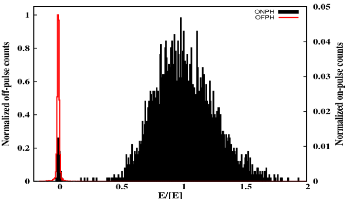
Figure A.1.: The ONPH and the OFPH for PSR B0809+74 observed at 325 MHz. The on-pulse and the off-pulse energies were binned in around 500 bins. Note the clear bimodal distribution of the ONPH due to the small fraction of null pulses.

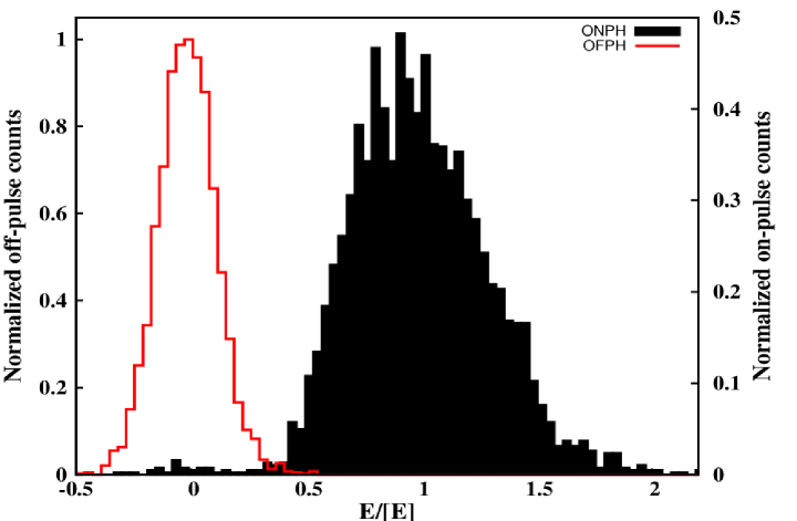
Figure A.2.: The ONPH and the OFPH for PSR B0818$-$13 observed at 610 MHz. The on-pulse and the off-pulse energies were binned in around 100 bins. The ONPH does not show very clear separation of null and burst pulses due to the weak burst pulses.

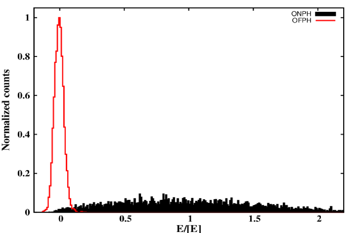
Figure A.3.: The ONPH and the OFPH for PSR B0835$-$41 observed at 610 MHz. The on-pulse and the off-pulse energies were binned in around 300 bins. The ONPH does not show very clear separation of null and burst pulses due to the weak burst pulses.

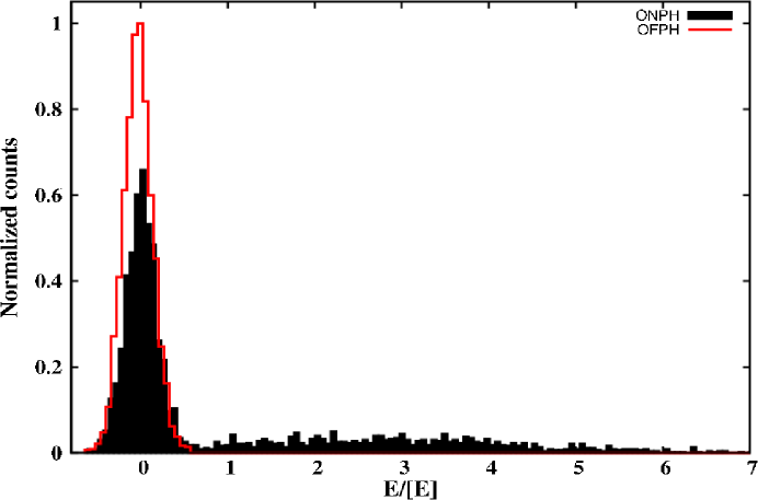
Figure A.4.: The ONPH and the OFPH for PSR B1112+50 observed at 325 MHz. The on-pulse and the off-pulse energies were binned in around 200 bins. The ONPH does show a very clear bimodal distribution due to the mixture of null pulses and burst pulses.

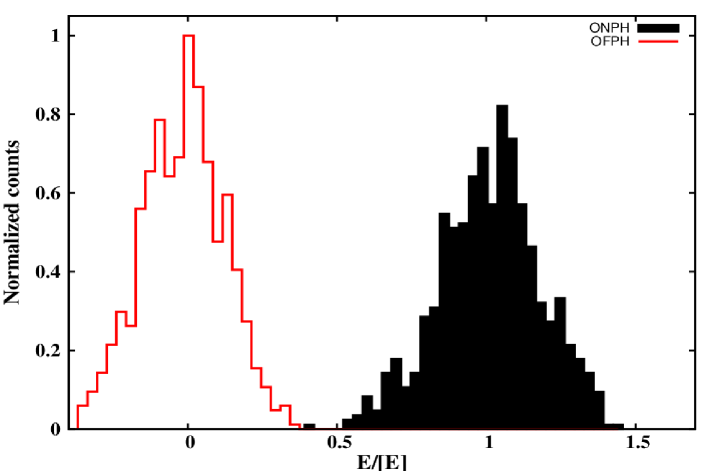
Figure A.5.: The ONPH and the OFPH for PSR J1639$-$4359 observed at 610 MHz. The on-pulse and the off-pulse energies were binned in around 100 bins. To obtain these histograms, successive 5 pulses were sub-integrated (see Section 4.2). The NF, displayed in the inset texts, was estimated by arranging single pulses in the ascending order of their on-pulse energy and separating low energy single pulses. These histograms are presented here to demonstrate absence of null pulses among the sub-integrated pulses.

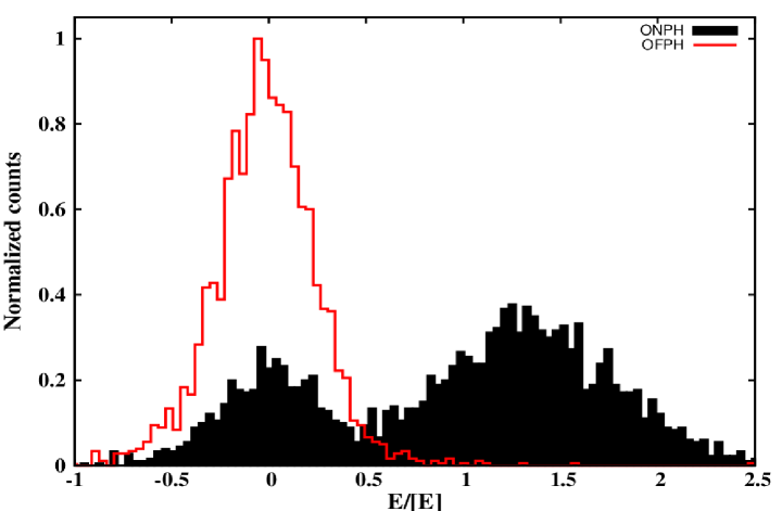
Figure A.6.: The ONPH and the OFPH for PSR B1658$-$37 observed at 610 MHz. The on-pulse and the off-pulse energies were binned in around 200 bins. The ONPH does show very clear bimodal distribution originating from the null pulses and relatively stronger burst pulses.

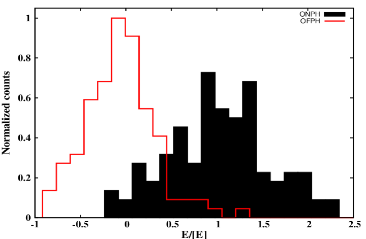
Figure A.7.: The ONPH and the OFPH for PSR J1715$-$4034 observed at 610 MHz. The on-pulse and the off-pulse energies were binned in around 25 bins. To obtain these histograms, successive 10 pulses were sub-integrated (see Section 4.2). Thus, NF shown in the inset text, is only a lower limit on the true NF.

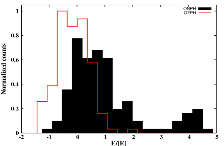
Figure A.8.: The ONPH and the OFPH for PSR J1725$-$4043 observed at 610 MHz. The on-pulse and the off-pulse energy were binned in around 20 bins. To obtain these histograms, successive 24 pulses were sub-integrated (see Section 4.2). The ONPH shows mixture of true null pulses and weak Mode B pulses near the zero pulse energy. The on-pulse energy from strong Mode A pulses clearly shows distribution away from the zero pulse energy.

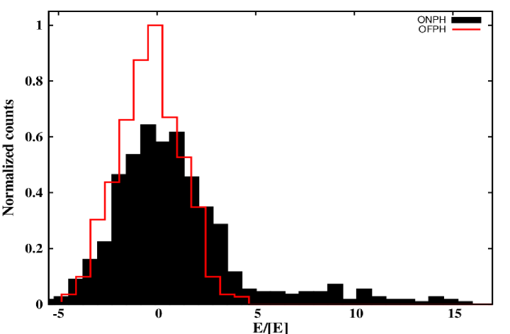
Figure A.9.: The ONPH and the OFPH for PSR J1738$-$2330 observed at 325 MHz. The on-pulse and the off-pulse energies were binned in around 40 bins. To obtain these histograms, successive 5 pulses were sub-integrated (see Section 4.2). The ONPH shows a large fraction of null pulses.

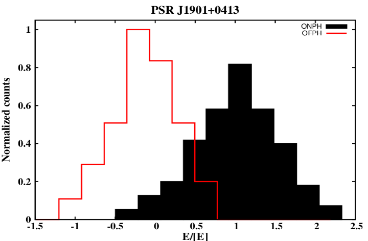
Figure A.10.: The ONPH and the OFPH for PSR J1901+0413 observed at 610 MHz. The on-pulse and the off-pulse energies were binned in around 15 bins. To obtain these histograms, successive 10 pulses were sub-integrated (see Section 4.2). The NF, displayed in the inset texts, was estimated by arranging single pulses in the ascending order of their on-pulse energy and separating low energy single pulses. These histograms are presented here to demonstrate small fraction of null pulses among the sub-integrated pulses.

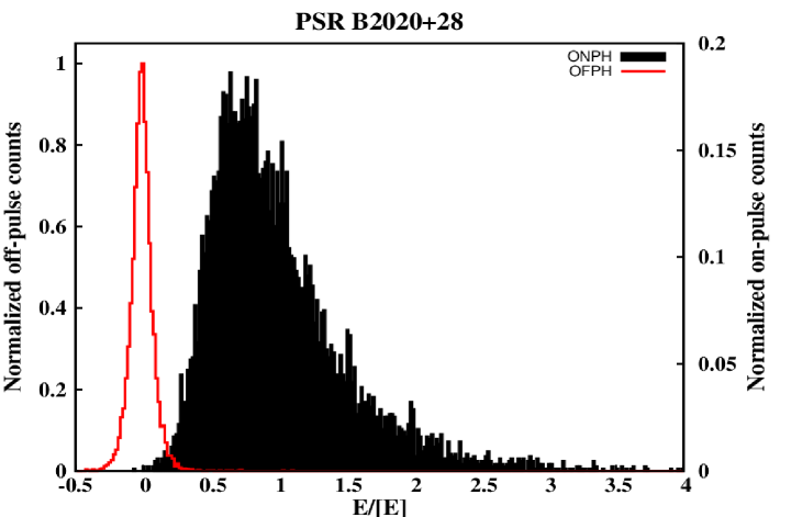
Figure A.11.: The ONPH and the OFPH for PSR B2020+28 observed at 610 MHz. The on-pulse and the off-pulse energies were binned in around 300 bins. The obtained NF along with the number of pulses used during the analysis are displayed in the inset texts.

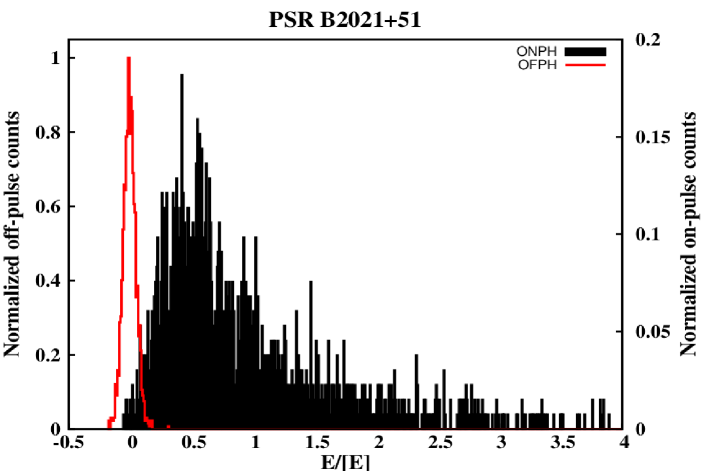
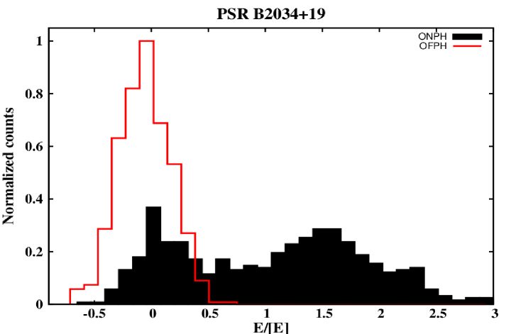
Figure A.12.: The ONPH and the OFPH for PSR B2021+51 observed at 610 MHz. The on-pulse and the off-pulse energies were binned in around 800 bins. The obtained NF along with the number of pulses used during the analysis are displayed in the inset texts.

Figure A.13.: The ONPH and the OFPH for PSR B2034+19 observed at 610 MHz. The on-pulse and the off-pulse energies were binned in around 30 bins. To obtain these histograms, successive 3 pulses were sub-integrated (see Section 4.2). The ONPH shows clear bi-modal distribution of the on-pulse energy in the sub-integrated data originating from the null pulses and burst pulses.

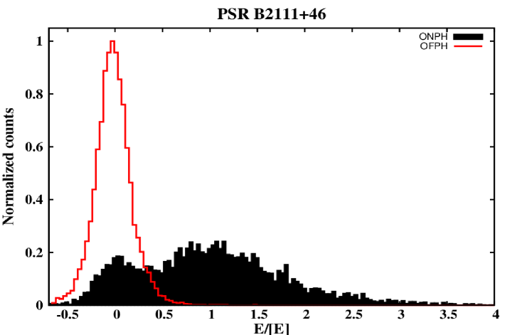
Figure A.14.: The ONPH and the OFPH for PSR B2111+46 observed at 610 MHz. The on-pulse and the off-pulse energies were binned in around 200 bins. The obtained NF along with the number of pulses used during the analysis are displayed in the inset texts.

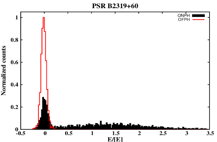
Figure A.15.: The ONPH and the OFPH for PSR B2319+60 observed at 610 MHz. The on-pulse and the off-pulse energies were binned in around 200 bins. The obtained NF along with the number of pulses used during the analysis are displayed in the inset texts.

Appendix B Appendix B
Null length and Burst length histograms

This Appendix lists all the null length and the burst length histograms obtained for pulsars studied in Chapter 4. The NLHs are shown in the left hand panel with red solid line while the BLHs are shown on the right hand panel with blue sold line. The abscissa present length of contiguous null or burst phases in units of pulsar periods. The ordinate presents the normalized counts as counts on every bin were normalized by the total number of observed contiguous null/burst lengths (mentioned in the caption) for each pulsar. The pulsar names are given at the top of the plot.

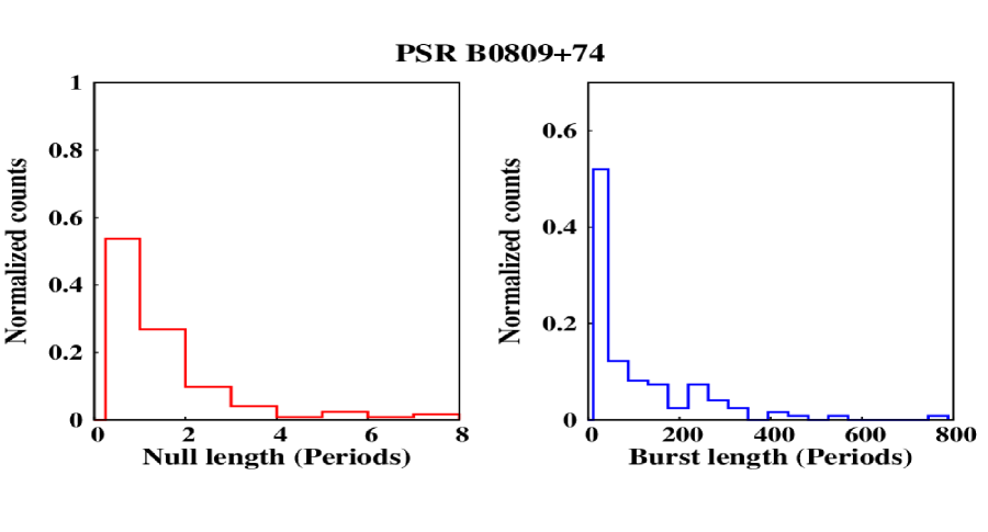
Figure B.1.: The NLH and BLH for PSR B0809+74. Total 73 null lengths and 73 burst lengths were included to construct these histograms.

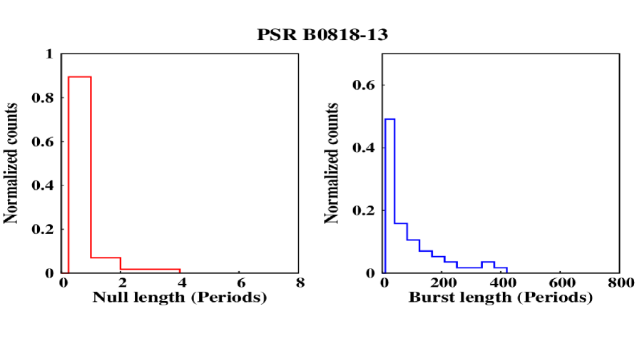
Figure B.2.: The NLH and BLH for PSR B0818$-$13. Total 57 null lengths and 57 burst lengths were included to construct these histograms.

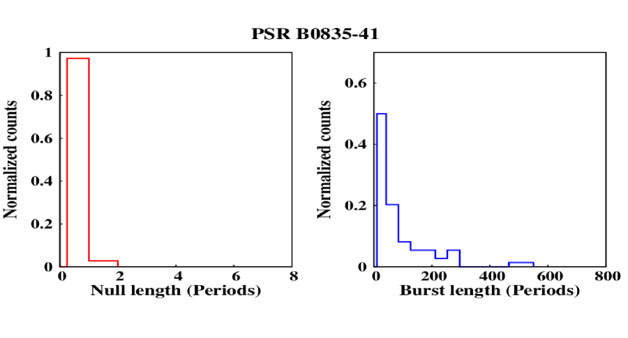
Figure B.3.: The NLH and BLH for PSR B0835$-$41. Total 74 null lengths and 74 burst lengths were included to construct these histograms.

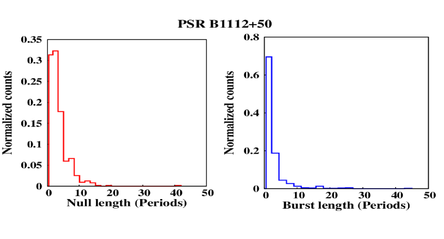
Figure B.4.: The NLH and BLH for PSR B1112+50. Total 635 null lengths and 635 burst lengths were included to construct these histograms.

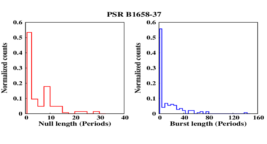
Figure B.5.: The NLH and BLH for PSR B1658$-$37. Total 73 null lengths and 73 burst lengths were included to construct these histograms.

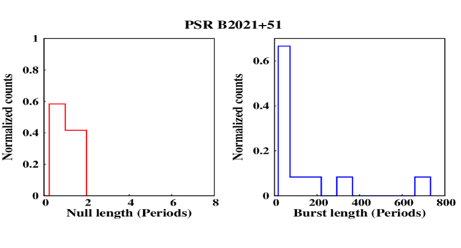
Figure B.6.: The NLH and BLH for PSR B2021+51. Total 12 null lengths and 12 burst lengths were included to construct these histograms.

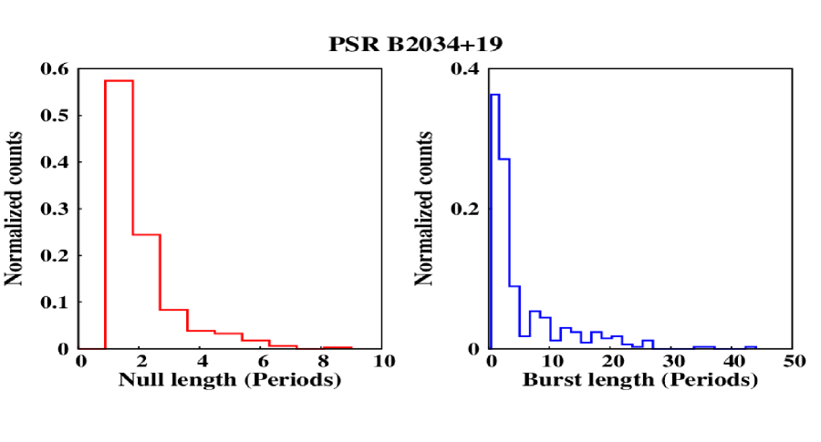
Figure B.7.: The NLH and BLH for PSR B2034+19. Total 336 null lengths and 336 burst lengths were included to construct these histograms.

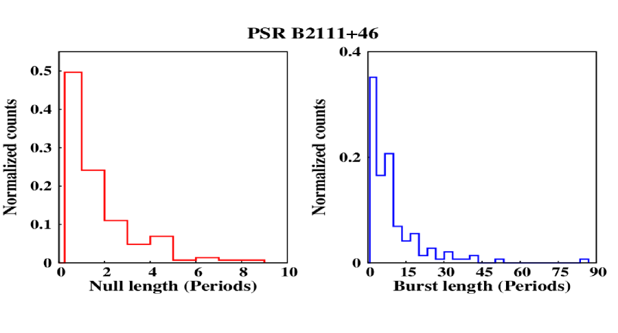
Figure B.8.: The NLH and BLH for PSR B2111+46. Total 145 null lengths and 145 burst lengths were included to construct these histograms.

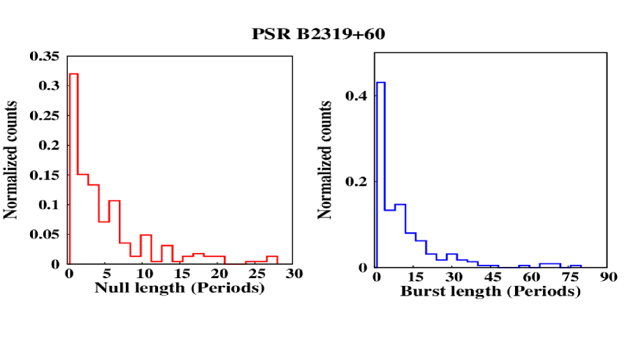
Figure B.9.: The NLH and BLH for PSR B2319+60. Total 225 null lengths and 225 burst lengths were included to construct these histograms.

Appendix C Appendix C
Cumulative Distribution Function

This appendix displays the Cumulative distribution functions (CDF), as discussed in Chapter 4, of eight pulsars for which the NLH and the BLH were possible to obtain. PSR B1658$-$37 did not show a suitable match with the fitted model, hence it was not included in the following plots. Moreover, for PSRs B0837$-$41 and B2021+51 the null length distribution only showed single and double period nulls, hence they were also excluded in the following plots. For each pulsars, both the null length and burst length fits to the Poisson point process, given by the following equation, are shown.

$$F(x)=1-\exp{(-x/\tau)}$$ (C.1)

Each plot shows the obtained CDFs (blue line) using the observed null/burst length distributions along with the fitted models (red line). After obtaining the least-square-fit, the decay parameter, $\tau$, was obtained for each CDF. These fitted parameters, $\tau_{n}$ and $\tau_{b}$ in units of pulsar period ($P_{1}$), are also shown for each pulsar. The fitted model was checked by carrying out a two-sample KS-test between the observed CDF and the obtained CDF from the simulated data, as discussed in Section 4.5. The rejection probability of the null hypothesis of similar distributions is also shown for each pulsar in the inset texts.

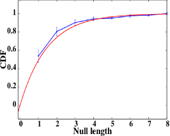
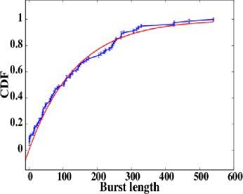
Figure C.1.: Null length and burst length CDFs for PSR B0809+74

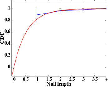
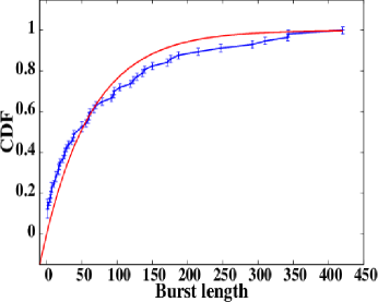
Figure C.2.: Null length and burst length CDFs for PSR B0818$-$13

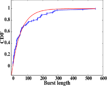
Figure C.3.: Null length and burst length CDFs for PSR B0837$-$41

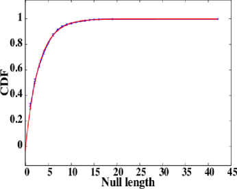
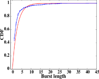
Figure C.4.: Null length and burst length CDFs for PSR B1112+50

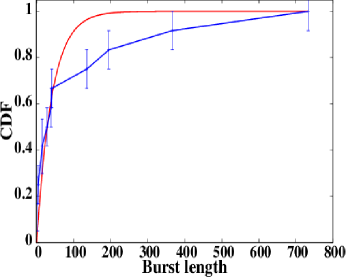
Figure C.5.: Null length and burst length CDFs for PSR B2021+51

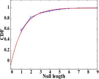
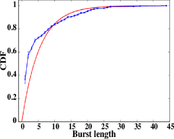
Figure C.6.: Null length and burst length CDFs for PSR B2034+19

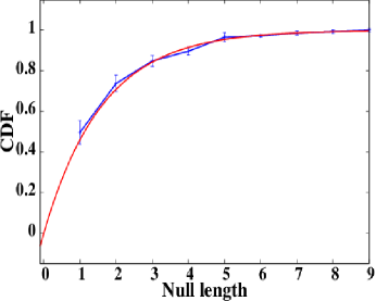
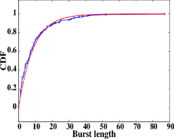
Figure C.7.: Null length and burst length CDFs for PSR B2111+46

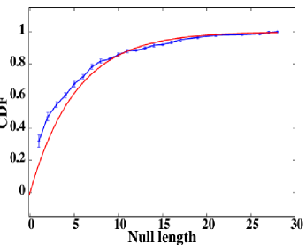
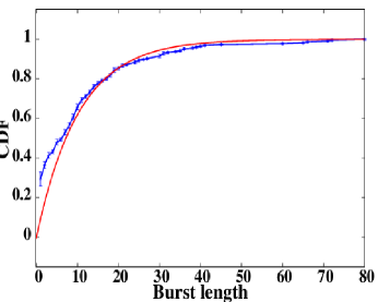
Figure C.8.: Null length and burst length CDFs for PSR B2319+60

Appendix D Appendix D
The Pair Correlation Function

The Pair Correlation Function (PCF) is a probability density function (also known as the radial distribution function or pair separation function) for the clustering of certain objects or events in space and/or time coordinates Pimbley & Lu (1985) and is useful for measuring the degree of packing. We have used a one-dimensional PCF, which identifies the clustering of events (the bursts pulses of a bright phase in our case), in the time series data. A brief description is provided here as this seems to be the first time such a technique is applied the clustering of burst pulses in pulsar astronomy.

The PCF for a series M pulses with N burst pulses can be derived as follows. The pulse index of these burst pulses are

$$p_{i}~{}or~{}p_{j}~{}=~{}p_{1},~{}p_{2},~{}...,~{}p_{N}.$$ (D.1)

Then, PCF is defined as

$$g(p)~{}=~{}G\cdot\sum\limits_{i=1}^{N}\sum\limits_{j\neq{i}}^{N}\langle{\delta(p~{}-~{}\arrowvert{p_{j}-p_{i}}\arrowvert)}\rangle.$$ (D.2)

where G is a scaling parameter and $\delta$ is the Kronecker delta function. A normalized binning of PCF, g(p), provides the probability of occurrence of certain separations between burst pulses. If a pulsar exhibits bunching of burst pulses and periodic occurrence of these bunches, the PCF shows prominent peaks around repeatedly occurring separations and their harmonics. A simple way to detect such periodicities is to obtain the Fourier spectra of the PCF.

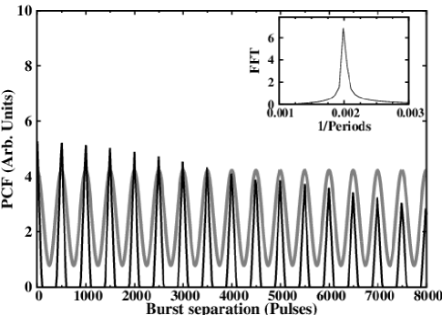
Figure D.1.: PCF of a pulsar whose nulls form clusters of 100 pulses separated by 400 periods. It is a histogram of the separations between the simulated burst pulses in units of pulse periods. Note the gradual reduction in amplitude for large separations due to the finite length of the simulated data. The inset figure shows the Fourier spectra of the PCF. A sine-wave with a 500 pulse periodicity is overlaid along with the PCF in grey colour for clarity.

Fig. D.1 shows an example of the PCF obtained for 8000 pulses of a pulsar nulling with a precise periodicity. The pulsar was simulated by repeated occurrence of 100 burst pulses separated by 400 null pulses, so the NF was 80 %. The periodicity is clearly visible both in the PCF and in the Fourier spectra in the inset figure. The peaks in PCF are at 500 pulses, broadened by the 100 pulse spread.

The PCF measures not only the periodicity of the clustering but also how long its coherence persists. If coherence in the bunching is lost, the PCF would not show peaks beyond a particular length. This makes it superior to a simple Fourier analysis of the pulse energy modulation since a PCF emphasises short-lived periodic features as well as providing information regarding the coherence length. An additional advantage over conventional Fourier analysis is that observations from different sessions can be combined. The maximum coherence length measurable in this case will come from the session with the longest pulse sequence among all the observing sessions. Hence, the PCF is a useful technique to scrutinize periodic pulse energy fluctuations.

References

- Akujor & Okeke (1982) Akujor C. E., Okeke P. N., 1982, Ap&SS, 85, 325
- Arons (1981) Arons J., 1981, ApJ, 248, 1099
- Arons (1983) Arons J., 1983, in Burns M. L., Harding A. K., Ramaty R., eds, Positron-Electron Pairs in Astrophysics Vol. 101 of American Institute of Physics Conference Series, Electron positron pairs in radio pulsars. pp 163–193
- Arons (1983) Arons J., 1983, ApJ, 266, 215
- Arons & Barnard (1986) Arons J., Barnard J. J., 1986, ApJ, 302, 120
- Arons & Scharlemann (1979) Arons J., Scharlemann E. T., 1979, ApJ, 231, 854
- Asseo et al. (1990) Asseo E., Pelletier G., Sol H., 1990, MNRAS, 247, 529
- Baade & Zwicky (1934) Baade W., Zwicky F., 1934, Physical Review, 46, 76
- Baars & Hooghoudt (1974) Baars J. W. M., Hooghoudt B. G., 1974, A&A, 31, 323
- Backer (1970a) Backer D. C., 1970a, Nat., 228, 752
- Backer (1970b) Backer D. C., 1970b, Nat., 228, 1297
- Backer (1970c) Backer D. C., 1970c, Nat., 228, 42
- Backer (1976) Backer D. C., 1976, ApJ, 209, 895
- Backus et al. (2010) Backus I., Mitra D., Rankin J. M., 2010, MNRAS, 404, 30
- Backus (1981) Backus P. R., 1981, PhD thesis, The University of Massachusetts
- Bartel & Sieber (1978) Bartel N., Sieber W., 1978, A&A, 70, 307
- Bartel et al. (1980) Bartel N., Sieber W., Wolszczan A., 1980, 90, 58
- Baym (1991) Baym G., 1991, in Ventura J., Pines D., eds, NATO ASIC Proc. 344: Neutron Stars Vol. 334, The High Density Interiors of Neutron Stars. p. 21
- Bell-Burnell (1977) Bell-Burnell S. J., 1977, in Papagiannis M. D., ed., Eighth Texas Symposium on Relativistic Astrophysics Vol. 302 of Annals of the New York Academy of Sciences, Petit Four. p. 685
- Benford & Buschauer (1977) Benford G., Buschauer R., 1977, MNRAS, 179, 189
- Beskin et al. (1988) Beskin V. S., Gurevich A. V., Istomin I. N., 1988, Ap&SS, 146, 205
- Bhat et al. (2007) Bhat N. D. R., Gupta Y., Kramer M., Karastergiou A., Lyne A. G., Johnston S., 2007, A&A, 462, 257
- Bhattacharyya et al. (2008) Bhattacharyya B., Gupta Y., Gil J., 2008, MNRAS, 383, 1538
- Bhattacharyya et al. (2010) Bhattacharyya B., Gupta Y., Gil J., 2010, MNRAS, 408, 407
- Biggs (1992) Biggs J. D., 1992, ApJ, 394, 574
- Biggs et al. (1985) Biggs J. D., McCulloch P. M., Hamilton P. A., Manchester R. N., Lyne A. G., 1985, MNRAS, 215, 281
- Blandford (1975) Blandford R. D., 1975, MNRAS, 170, 551
- Burke-Spolaor & Bailes (2010) Burke-Spolaor S., Bailes M., 2010, MNRAS, 402, 855
- Burke-Spolaor et al. (2011) Burke-Spolaor S., Bailes M., Johnston S., Bates S. D., Bhat N. D. R., Burgay M., D’Amico N., Jameson A., Keith M. J., Kramer M., Levin L., Milia S., Possenti A., Stappers B., van Straten W., 2011, MNRAS, 416, 2465
- Burke-Spolaor et al. (2012) Burke-Spolaor S., Johnston S., Bailes M., Bates S. D., Bhat N. D. R., Burgay M., Champion D. J., D’Amico N., Keith M. J., Kramer M., Levin L., Milia S., Possenti A., Stappers B., van Straten W., 2012, MNRAS, 423, 1351
- Cadez et al. (1997) Cadez A., Galicic M., Calvani M., 1997, A&A, 324, 1005
- Camilo et al. (2012) Camilo F., Ransom S. M., Chatterjee S., Johnston S., Demorest P., 2012, ApJ, 746, 63
- Chen & Ruderman (1993) Chen K., Ruderman M., 1993, ApJ, 408, 179
- Cheng (1981) Cheng A. F., 1981, in Sieber W., Wielebinski R., eds, Pulsars: 13 Years of Research on Neutron Stars Vol. 95 of IAU Symposium, Observational consequences of polar CAP theories. pp 99–101
- Cheng & Ruderman (1977) Cheng A. F., Ruderman M., 1977, ApJ, 212, 800
- Clemens & Rosen (2004) Clemens J. C., Rosen R., 2004, ApJ, 609, 340
- Cole (1970) Cole T. W., 1970, Nat., 227, 788
- Contopoulos (2005) Contopoulos I., 2005, A&A, 442, 579
- Contopoulos et al. (1999) Contopoulos I., Kazanas D., Fendt C., 1999, ApJ, 511, 351
- Cordes (1978) Cordes J. M., 1978, ApJ, 222, 1006
- Cordes (1981) Cordes J. M., 1981, in Sieber W., Wielebinski R., eds, Pulsars, IAU Symposium 95 Radio observational constraints on pulsar emission mechanisms. Reidel, Dordrecht, p. 115
- Cordes (1983) Cordes J. M., 1983, in Burns M. L., Harding A. K., Ramaty R., eds, Positron-Electron Pairs in Astrophysics Vol. 101 of American Institute of Physics Conference Series, Radio pulsars - Intensity, polarization, and rotation fluctuations. pp 98–112
- Cordes (2013) Cordes J. M., 2013, ApJ, 775, 47
- Cordes et al. (2004) Cordes J. M., Bhat N. D. R., Hankins T. H., McLaughlin M. A., Kern J., 2004, ApJ, 612, 375
- Cordes & Lazio (2002) Cordes J. M., Lazio T. J. W., 2002, ArXiv Astrophysics e-prints
- Cordes & Shannon (2008) Cordes J. M., Shannon R. M., 2008, ApJ, 682, 1152
- Crawford & Lorimer (2007) Crawford F., Lorimer D. R., 2007, ATNF Proposal, p. 1104
- Daugherty & Harding (1986) Daugherty J. K., Harding A. K., 1986, ApJ, 309, 362
- Davies et al. (1984) Davies J. G., Lyne A. G., Smith F. G., Izvekova V. A., Kuzmin A. D., Shitov Y. P., 1984, MNRAS, 211, 57
- Deich et al. (1986) Deich W. T. S., Cordes J. M., Hankins T. H., Rankin J. M., 1986, ApJ, 300, 540
- Deneva et al. (2009) Deneva J. S., Cordes J. M., McLaughlin M. A., Nice D. J., Lorimer D. R., Crawford F., Bhat N. D. R., Camilo F., Champion D. J., Freire P. C. C., Edel S., Kondratiev V. I., Hessels J. W. T., 2009, ApJ, 703, 2259
- Deshpande & Rankin (1999) Deshpande A. A., Rankin J. M., 1999, ApJ, 524, 1008
- Deshpande & Rankin (2001) Deshpande A. A., Rankin J. M., 2001, MNRAS, 322, 438
- Deutsch (1955) Deutsch A. J., 1955, Annales d’Astrophysique, 18, 1
- Dewey et al. (1988) Dewey R. J., Taylor J. H., Maguire C. M., Stokes G. H., 1988, ApJ, 332, 762
- Dhillon et al. (2011) Dhillon V. S., Keane E. F., Marsh T. R., Stappers B. W., Copperwheat C. M., Hickman R. D. G., Jordan C. A., Kerry P., Kramer M., Littlefair S. P., Lyne A. G., Mignani R. P., Shearer A., 2011, MNRAS, 414, 3627
- Drake & Craft (1968) Drake F. D., Craft H. D., 1968, Nat., 220, 231
- Durdin et al. (1979) Durdin J. M., Large M. I., Little A. G., Manchester R. N., Lyne A. G., Taylor J. H., 1979, MNRAS, 186, 39P
- Dyks et al. (2005) Dyks J., Zhang B., Gil J., 2005, ApJ, 626, L45
- Ershov & Kuzmin (2005) Ershov A. A., Kuzmin A. D., 2005, A&A, 443, 593
- Esamdin et al. (2005) Esamdin A., Lyne A. G., Graham-Smith F., Kramer M., Manchester R. N., Wu X., 2005, MNRAS, 356, 59
- Faulkner et al. (2004) Faulkner A. J., Stairs I. H., Kramer M., Lyne A. G., Hobbs G., Possenti A., Lorimer D. R., Manchester R. N., McLaughlin M. A., D’Amico N., Camilo F., Burgay M., 2004, MNRAS, 355, 147