Towards an effective field theory approach to the neutrinoless double-beta decay

Abstract

Weak interaction in nuclei represents a well-known venue for testing many of the fundamental symmetries of the Standard Model. In particular, neutrinoless double-beta decay offers the possibility to test Beyond Standard Model theories predicting that neutrinos are Majorana fermions and the lepton number conservation is violated. This paper focuses on an effective field theory approach to neutrinoless double-beta decay for extracting information regarding the properties of the Beyond Standard Model Lagrangian responsible for this process. We use shell model nuclear matrix elements and the latest experimental lower limits for the half-lives to extract the lepton number violating parameters of five nuclei of experimental interest, and lower limits for the energy scales of the new physics.

I Introduction

The neutrinoless double-beta decay ($0\nu\beta\beta$) is considered the best approach to study the yet unknown properties of neutrinos related to their nature, whether they are Dirac or Majorana fermions, which the neutrino oscillation experiments cannot clarify. Should the neutrinoless double-beta transitions occur, then the lepton number conservation is violated by two units, and the black-box theorems Schechter and Valle (1982); Nieves (1984); Takasugi (1984); Hirsch et al. (2006) indicate that the light left-handed neutrinos are Majorana fermions. As such, through black-box theorems alone, it is not possible to disentangle the dominant mechanism contributing to this process. Most of the theoretical effort dedicated to this subject consists of calculations of leptonic phase-space factors and nuclear matrix elements that are computed via several nuclear structure methods and within specific models. One of the most popular models is the left-right symmetric model Pati and Salam (1974); Mohapatra and Pati (1975a); Senjanovic and Mohapatra (1975); Keung and Senjanovic (1983); Barry and Rodejohann (2013), which is currently investigated at the Large Hadron Collider (LHC) Khachatryan et al. (2014). In two recent papers Horoi and Neacsu (2016a); Neacsu and Horoi (2016) we have discussed ways to identify some of the possible contributions to the decay rate by studying the angular distribution and the energy distribution of the two outgoing electrons that could be measured. However, there are still many other possible contributions to this process that one cannot yet dismiss. For these reasons, a more general beyond standard model (BSM) effective field theory would be preferable, as it would not be limited to relying on specific models, but rather considering the most general BSM effective field theoretical approach that describes this process. An important outcome of such a theory is the evaluation of the energy scales up to which the effective field operators are not broken, together with limits for the effective low-energy couplings.

The analysis of the $0\nu\beta\beta$ decay process is generally done at three levels. At the lowest level the weak interaction of the quarks and leptons is considered and the BSM physics is treated within a low-energy effective field theory approach. At the next level the hadronization process to nucleons and exchanging pion is considered. The nucleons are treated in the impulse approximation leading to free space $0\nu\beta\beta$ transition operators. At the third level the nucleon dynamics inside the nuclei is treated using nonperturbative nuclear wave functions, which are further used to obtain nuclear matrix elements (NME) needed to calculate the $0\nu\beta\beta$ observables, such as half-lives and two-electron angular and energy distributions Horoi and Neacsu (2016a). A modern approach that could accomplish this plan would based on the chiral effective field theory of pions and nucleons Cirigliano et al. (2017a, b). This approach introduces a number of couplings, which in principle can be calculated from the underlying theory of strong interaction using lattice QCD techniques Cirigliano et al. (2017a), or may be extracted within some approximation from the known experimental data Cirigliano et al. (2017b). These couplings may come with new phases and they may include effective contributions from the exchange of heavier mesons. The lattice QCD approach is underway, but it proved to be very difficult for extracting even basic weak nucleon couplings, such as $g_{A}$ Berkowitz et al. (2017).

In this paper we start from the formalism of Ref. Hirsch et al. (1996a); Pas et al. (1999, 2001); Deppisch et al. (2012) that provides a general effective field theory (EFT) approach to the neutrinoless double-beta decay. However, at the hadron level three new diagrams are added for the first time to the effective field theory analysis of the $0\nu\beta\beta$, which were only considered in the literature in the context of specific mechanisms. Under the assumption that a single coupling in the BSM Lagrangian dominates the $0\nu\beta\beta$ amplitude, we extract new limits for the effective Majorana mass and for 11 additional low-energy EFT couplings using data from five nuclei of current experimental interest. Some of these couplings correspond to parameters found in left-right symmetric models, and we present and compare them. To be able to get the limits of these effective couplings and parameters from the experimental half-life limits, 23 nuclear matrix elements (NME) and 9 phase-space factors (PSF) are needed. Finally, we use the limits for the EFT couplings and the formalism of the effective field theory to obtain limits for the energy scale of the new physics that could be responsible for the neutrinoless double beta decay process.

To accomplish this goal we need reliable NME. The most commonly used nuclear structure methods for the NME calculation are proton-neutron Quasi Random Phase Approximation (pnQRPA) Hirsch et al. (1996a); Pas et al. (1999, 2001); Deppisch et al. (2012); Simkovic et al. (1999); Suhonen and Civitarese (2010); Faessler et al. (2011); Mustonen and Engel (2013); Faessler et al. (2014), Interacting Shell Model (ISM) Retamosa et al. (1995); Caurier et al. (1996); Horoi (2013); Neacsu and Stoica (2014a); Caurier et al. (2008); Menendez et al. (2009); Caurier et al. (2005); Horoi and Stoica (2010); Neacsu et al. (2012); Sen’kov and Horoi (2013); Horoi and Brown (2013); Sen’kov et al. (2014); Brown et al. (2014); Neacsu and Stoica (2014b); Sen’kov and Horoi (2014); Neacsu and Horoi (2015); Horoi and Neacsu (2016b); Horoi et al. (2007); Blennow et al. (2010), Interacting Boson Model (IBM-2) Barea and Iachello (2009); Barea et al. (2012, 2013, 2015), Projected Hartree Fock Bogoliubov (PHFB) Rath et al. (2013), Energy Density Functional (EDF) Rodriguez and Martinez-Pinedo (2010), and the Relativistic Energy Density Functional (REDF) Song et al. (2014) method. The NME calculated with different methods and by different groups sometimes show large differences, and this has been debated in the literature Faessler et al. (2012); Vogel (2012). Although there seem to exist many NME results to choose from, most of the references listed only provide calculations for the light left-handed Majorana neutrino exchange. Ref. Horoi and Neacsu (2016b) provides tables and plots that compare the latest results for the light left-handed neutrino exchange and for the heavy right-handed neutrino exchange.

The NME used in Ref. Hirsch et al. (1996a); Pas et al. (1999, 2001); Deppisch et al. (2012) come from older QRPA calculations, which do not include many of the improvements proposed in recent years Simkovic et al. (2013); Hyvarinen and Suhonen (2015). We calculate the NME using shell model techniques, which are consistent with previous calculations Horoi et al. (2007); Horoi and Stoica (2010); Neacsu et al. (2012); Horoi and Brown (2013); Neacsu and Stoica (2014b); Sen’kov and Horoi (2013); Horoi (2013); Brown et al. (2014); Sen’kov and Horoi (2014); Sen’kov et al. (2014); Neacsu and Horoi (2015); Horoi and Neacsu (2016b). The reason for choosing shell model NME is our belief that these are better suited and more reliable for $0\nu\beta\beta$ calculations, as they take into account all the correlations around the Fermi surface, respect all symmetries, and take into account consistently the effects of the missing single particle space via many-body perturbation theory (the effects were shown to be small, about 20%, for ⁸²Se Holt and Engel (2013)). Furthermore, we have tested the shell model methods and the effective Hamiltonians used by comparing calculations of spectroscopic observables to the experimental data, as presented in Ref. Horoi and Stoica (2010); Sen’kov and Horoi (2016); Horoi and Neacsu (2016b). We do not consider any quenching for the bare $0\nu\beta\beta$ operator in these calculations. Such a choice is different from that for the simple Gamow-Teller operator used in the single beta and $2\nu\beta\beta$ decays where a quenching factor of about 0.7 is necessary Brown et al. (2015). For the PSF we use an effective theory based on the formalism of Ref. Doi et al. (1985), but fine-tuned as to take into account the effects of a Coulomb field distorting finite-size proton distribution in the final nucleus. To our knowledge, some of the NME presented in this paper are calculated for the first time using shell model techniques.

This paper is organized as follows: Section II analyzes the contributions of several BSM mechanisms to the neutrinoless double-beta decay. Section III presents the framework of the effective field theory for the neutrinoless double-beta decay. Section IV shows the experimental limits on the BSM lepton number violating (LNV) couplings that we calculate, and is divided into three subsections. Subsection IV.1 is dedicated to the revisit of the most common approach to $0\nu\beta\beta$ that considers only the light left-handed Majorana neutrino exchange, presenting shell model nuclear matrix elements and upper limits for the Majorana mass. Subsection IV.2 details the study of the long-range contributions to the $0\nu\beta\beta$ decay Lagrangian. Subsection IV.3 presents the analysis of the short-range contribution LNV parameters. Discussions are presented in Section V, Section VI is dedicated to conclusions and, last, Section VII is an Appendix containing all the relevant formulae for calculating the NME.

Table 1: The $Q^{0\nu}_{\beta\beta}$ values in MeV, the experimental $T^{0\nu}_{1/2}$ limits in years, and the calculated PSF ($G_{01}-G_{09}$) in years^-1 for all five isotopes currently under investigation.

	48Ca	76Ge	82Se	130Te	136Xe
$Q^{0\nu}_{\beta\beta}$ Stoica and Mirea (2013)	4.272	2.039	2.995	2.813	2.287
$T^{0\nu}_{1/2}\ >$	$2.0\cdot 10^{22}$ Arnold et al. (2016)	$5.3\cdot 10^{25}$ Agostini et al. (2017)	$2.5\cdot 10^{23}$ Wat (2016)	$4.0\cdot 10^{24}$ Alfonso et al. (2015)	$1.07\cdot 10^{26}$ Gando et al. (2016)
$G_{01}\cdot 10^{14}$	$2.45$	$0.22$	$1.00$	$1.41$	$1.45$
$G_{02}\cdot 10^{14}$	$15.4$	$0.35$	$3.21$	$3.24$	$3.15$
$G_{03}\cdot 10^{15}$	$18.2$	$1.20$	$6.50$	$8.46$	$8.55$
$G_{04}\cdot 10^{15}$	$5.04$	$0.42$	$1.92$	$2.53$	$2.58$
$G_{05}\cdot 10^{13}$	$3.28$	$0.60$	$2.16$	$4.12$	$4.36$
$G_{06}\cdot 10^{12}$	$3.87$	$0.50$	$1.65$	$2.16$	$2.21$
$G_{07}\cdot 10^{10}$	$2.85$	$0.28$	$1.20$	$1.75$	$1.80$
$G_{08}\cdot 10^{11}$	$1.31$	$0.17$	$0.82$	$1.72$	$1.83$
$G_{09}\cdot 10^{10}$	$15.5$	$1.12$	$4.42$	$4.47$	$4.44$

II BSM mechanisms contributing to neutrinoless double-beta decay

The main mechanism considered to be responsible for the neutrinoless double beta decay is the mass mechanism that assumes that the neutrinos are Majorana fermions, and relies on the assumption that the light left-handed neutrinos have mass. However, the possibility that right-handed currents could contribute to the neutrinoless double-beta decay $(0\nu\beta\beta)$ has been already considered for some time Doi et al. (1983, 1985). Recently, $0\nu\beta\beta$ studies Rodejohann (2012); Barry and Rodejohann (2013) have adopted the left-right symmetric model Mohapatra and Pati (1975b); Senjanovic and Mohapatra (1975) for the inclusion of right-handed currents. In addition, the $R$-parity violating $(\cancel{\cal{R}}_{p})$ supersymmetric (SUSY) model can also contribute to the neutrinoless double beta decay process Hirsch et al. (1996b); Kolb et al. (1997); Faessler et al. (2008). In the framework of the left-right symmetric model and $R$-parity violating SUSY model, the $0\nu\beta\beta$ half-life can be written as a sum of products of PSF, BSM LNV parameters, and their corresponding NME Horoi and Neacsu (2016a):

$$\left[T^{0\nu}_{1/2}\right]^{-1}= \ G_{01}g^{4}_{A}\left|\eta_{0\nu}M_{0\nu}+\left(\eta^{L}_{N_{R}}+\eta^{R}_{N_{R}}\right)M_{0N}\right.$$

$$+ \left.\eta_{\tilde{q}}M_{\tilde{q}}+\eta_{\lambda^{\prime}}M_{\lambda^{\prime}}+\eta_{\lambda}X_{\lambda}+\eta_{\eta}X_{\eta}\right|^{2}.$$ (1)

Here, $G_{01}$ is a phase-space factor that can be calculated with good precision for most cases Suhonen and Civitarese (1998); Kotila and Iachello (2012); Stoica and Mirea (2013); Horoi and Neacsu (2016c), $g_{A}$ is the axial vector coupling constant, $\eta_{0\nu}=\frac{\left<m_{\beta\beta}\right>}{m_{e}}$, with $\left<m_{\beta\beta}\right>$ representing the effective Majorana neutrino mass, and $m_{e}$ the electron mass. $\eta^{L}_{N_{R}}$, $\eta^{R}_{N_{R}}$ are the heavy neutrino parameters with left-handed and right-handed currents, respectively Horoi (2013); Barry and Rodejohann (2013), $\eta_{\tilde{q}}$, $\eta_{\lambda^{\prime}}$ are $\cancel{\cal{R}}_{p}$ SUSY LNV parameters Vergados et al. (2012), $\eta_{\lambda}$, and $\eta_{\eta}$ are parameters for the so-called ”$\lambda-$” and ”$\eta-$mechanism”, respectively Barry and Rodejohann (2013). $M_{0\nu}$, $M_{0N}$, are the light and the heavy neutrino exchange NME, $M_{\tilde{q}}$, $M_{\lambda^{\prime}}$ are the $\cancel{\cal{R}}_{p}$ SUSY NME, and $X_{\lambda}$ and $X_{\eta}$ denote combinations of NME and other PSF ($G_{02}-G_{09}$) corresponding to the the $\lambda-$mechanism involving right-handed leptonic and right-handed hadronic currents, and the $\eta-$mechanism with right-handed leptonic and left-handed hadronic currents, respectively Horoi and Neacsu (2016a). The heavy neutrino exchange contribution to the amplitude in Eq. II proportional with $M_{N}$ assumes that the heavy neutrino masses are larger than $\approx\ 1$ GeV and the information about their mass is included into the couplingsHoroi and Neacsu (2016a).

In Table LABEL:tab-psf we present the $Q^{0\nu}_{\beta\beta}$ values, the most recent experimental half-life limits from the indicated references, and the nine PSF for $0\nu\beta\beta$ transitions to ground states of the daughter nucleus for five isotopes currently under investigation. The PSF were calculated using a new effective method described in great detail in Ref. Horoi and Neacsu (2016c). $G_{01}$ values were calculated with a screening factor ($s_{f}$) of 94.5, while for $G_{02}-G_{09}$ we used $s_{f}=92.0$ that was shown to provide results very close to those of Ref. Stefanik et al. (2015). We note that the ⁸²Se experimental half-life used here and throughout this analysis is preliminary Wat (2016). However, we believe that this limit is valid and that it may get improved.

In Ref. Horoi and Neacsu (2016a) we show how one could disentangle contributions form different mechanisms using two-electron angular and energy distributions, as well as half-life data from several isotopes. Here, we consider the case where one mechanism dominates, more explicitly, one single term in the decay amplitude of Eq. (II). Table LABEL:tab-etas shows the shell model values of the NME that enter Eq. (II). The light and heavy neutrino-exchange NME, $M_{0\nu}$ and $M_{0N}$, are taken from Ref. Neacsu and Horoi (2015) that describes their formalism and calculation. $M_{\tilde{q}}$ and $M_{\lambda^{\prime}}$ are calculated using the description in Eq. (150) and Eq. (155), respectively, of Ref. Vergados et al. (2012). $X_{\lambda}$ and $X_{\eta}$ are adapted from $C_{4}$ and $C_{5}$ of Eq. (3.5.15d) and Eq. (3.5.15e), respectively, in Ref. Doi et al. (1985) multiplied by $M_{GT}/G_{01}$ to fit the factorization of Eq. (II). All NME used in this paper were calculated using the interacting shell model (ISM) approach Blennow et al. (2010); Horoi (2013); Horoi and Brown (2013); Sen’kov et al. (2014); Sen’kov and Horoi (2013); Brown et al. (2014); Neacsu and Horoi (2015) (see Ref. Neacsu and Horoi (2015) for a review), and include short-range-correlation effects based on the CD-Bonn parametrization Horoi and Stoica (2010), finite-size effects Vergados et al. (2012) and, when appropriate, optimal closure energies Sen’kov and Horoi (2016) (see Appendix for more details).

The upper limits for corresponding LNV parameters extracted from lower limits of the half-lives under the assumption that only one term in the amplitude dominates, are also presented in Table LABEL:tab-etas. There are a few other QRPA Doi et al. (1985); Muto et al. (1989); Faessler and Simkovic (1998); Vergados et al. (2012); Stefanik et al. (2015) and ISM Retamosa et al. (1995); Caurier et al. (1996); Horoi (2013); Neacsu and Stoica (2014a) results in the literature that were obtained within the framework of the LRSM and SUSY. However, some of the extracted LNV parameters rely on some older half-life limits.

Table 2: The NME that appear in Eq. (II) for the five nuclei of current experimental interest, and the corresponding LNV parameters extracted under the assumption that only one dominates.

		48Ca	76Ge	82Se	130Te	136Xe
	$M_{0\nu}$	$1.03$	$3.64$	$3.41$	$1.93$	$1.75$
	$M_{0N}$	$75.5$	$202$	$187$	$136$	$122$
	$M_{\tilde{q}}$	$107$	$339$	$320$	$185$	$169$
	$M_{\lambda^{\prime}}$	$370$	$619$	$570$	$415$	$366$
	$X_{\lambda}$	$2.11$	$4.12$	$5.68$	$2.81$	$2.48$
	$X_{\eta}$	$246$	$794$	$725$	$517$	$467$
$10^{6}\cdot$	$\left|\eta_{0\nu}\right|$	$27.1$	$0.49$	$3.64$	$1.36$	$0.28$
$10^{9}\cdot$	$\left|\eta_{0N}\right|$	$370.6$	$8.83$	$66.3$	$19.2$	$4.01$
$10^{9}\cdot$	$\left|\eta_{\tilde{q}}\right|$	$260$	$5.26$	$38.8$	$14.1$	$2.91$
$10^{9}\cdot$	$\left|\eta_{\lambda^{\prime}}\right|$	$75.7$	$2.88$	$21.8$	$6.29$	$1.34$
$10^{7}\cdot$	$\left|\eta_{\lambda}\right|$	$133$	$4.32$	$21.87$	$9.29$	$1.98$
$10^{9}\cdot$	$\left|\eta_{\eta}\right|$	$114$	$2.25$	$17.1$	$5.05$	$1.05$

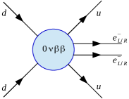
(a) The generic $0\nu\beta\beta$ decay diagram at the quark-level.

(b) Light left-handed neutrino exchange diagram.

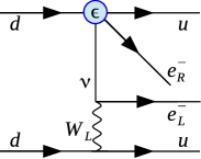
(c) The long-range part of the $0\nu\beta\beta$ diagram.

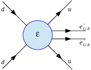
(d) The short-range part of the $0\nu\beta\beta$ diagram.

Figure 1: The $0\nu\beta\beta$ decay process diagrams: (1a) presents the generic description of the process, (1b) shows the most studied case in the literature, that of the light left-handed neutrino exchange, (1c) is the long-range component of the $0\nu\beta\beta$ decay diagram, while (1d) displays the short-range part.

III Effective field theory approach to neutrinoless double-beta decay

A more general approach is based on the effective field theory extension of the Standard Model. The analysis based on the BSM contributions to the effective field theory is more desirable, because it does not rely on specific models, and their parameters could be extracted/constrained by the existing $0\nu\beta\beta$ data, and by data from LHC and other experiments. In fact, the models considered in section II always lead to a subset of terms in the low-energy ($\sim$ 200 MeV) effective field theory Lagrangian. Here we consider all the terms in the Lagrangian allowed by the symmetries. Some of the couplings will correspond to the model couplings in Eq. (II), but they might have a wider meaning. Others are new, not corresponding to specific models.

At the quark-level, we present in Figure 1 the generic $0\nu\beta\beta$ Feynman diagrams contributing to the $0\nu\beta\beta$ process. We consider contributions coming from the light left-handed Majorana neutrino (Fig. 1b), a long-range part coming from the low-energy four-fermion charged-current interaction (Fig. 1c), and a short-range part (Fig. 1d).

We treat the long-range component of the $0\nu\beta\beta$ diagram as two point-like vertices at the Fermi scale, which exchange a light neutrino. In this case, the dimension 6 Lagrangian can be expressed in terms of effective couplings Deppisch et al. (2012):

$$\mathcal{L}_{6}=\frac{G_{F}}{\sqrt{2}}\left[j^{\mu}_{V-A}J^{\dagger}_{V-A,\mu}+\sum^{*}_{\alpha,\beta}\epsilon_{\alpha}^{\beta}j_{\beta}J^{\dagger}_{\alpha}\right],$$ (2)

where $J^{\dagger}_{\alpha}=\bar{u}\mathcal{O}_{\alpha}d$ and $j_{\beta}=\bar{e}\mathcal{O}_{\beta}\nu$ are hadronic and leptonic Lorentz currents, respectively. The definitions of the $\mathcal{O}_{\alpha,\beta}$ operators are given in Eq. (3) of Ref. Deppisch et al. (2012). The LNV parameters are $\epsilon_{\alpha}^{\beta}=\{\epsilon^{V+A}_{V-A},\ \epsilon^{V+A}_{V+A},\ \epsilon^{S+P}_{S\pm P},\ \epsilon^{TR}_{TL},\ \epsilon^{TR}_{TR}\}$. The ”*” symbol indicates that the term with $\alpha=\beta=(V-A)$ is explicitly taken out of the sum. However, the first term in Eq. (2) still entails BSM physics through the dimension-5 operator responsible for the Majorana neutrino mass (see also section V). Here $G_{F}=1.1663787\times 10^{-5}$ GeV^-2 denotes the Fermi coupling constant.

As already mentioned, some of these couplings play the same role as some of the model couplings listed in Eq. (II), but they have more general meaning here. For example, $\epsilon^{V+A}_{V-A}$ play the same role as $\eta_{\eta}$ and $\epsilon^{V+A}_{V+A}$ play the same role as $\eta_{\lambda}$ in the effective Lagrangian associated to models.

In the short-range part of the diagram presented in Fig. 1d we consider the interaction to be point-like. Expressing the general Lorentz-invariant Lagrangian in terms of effective couplings Pas et al. (2001), we get:

$$\mathcal{L}_{9}= \frac{G_{F}^{2}}{2m_{p}}\Bigl{[}\varepsilon_{1}JJj+\varepsilon_{2}J^{\mu\nu}J_{\mu\nu}j+\varepsilon_{3}J^{\mu}J_{\mu}j\Bigr{.}$$

$$+ \Bigl{.}\varepsilon_{4}J^{\mu}J_{\mu\nu}j^{\nu}+\varepsilon_{5}J^{\mu}Jj_{\mu}\Bigr{]},$$ (3)

with the hadronic currents of defined chirality $J=\bar{u}(1\pm\gamma_{5})d$, $J^{\mu}=\bar{u}\gamma^{\mu}(1\pm\gamma_{5})d$, $J^{\mu\nu}=\bar{u}\frac{i}{2}[\gamma^{\mu},\gamma^{\nu}](1\pm\gamma_{5})d$, leptonic currents $j=\bar{e}(1\pm\gamma_{5})e^{C}$, $j^{\mu}=\bar{e}\gamma^{\mu}(1\pm\gamma_{5})e^{C}$, and $\varepsilon_{\alpha}^{\beta}=\varepsilon_{\alpha}^{xyz}=\{\varepsilon_{1},\ \varepsilon_{2},\ \varepsilon_{3}^{LLz(RRz)},\ \varepsilon_{3}^{LRz(RLz)},\ \varepsilon_{4},\ \varepsilon_{6}\}$. These parameters have dependence on the chirality of the hadronic and the leptonic currents involved, with $xyz=L/R,L/R,L/R$. In the case of $\varepsilon_{3}$, one can distinguish between different chiralities, thus we express them separately as $\varepsilon_{3}^{LLz(RRz)}$ and $\varepsilon_{3}^{LRz(RLz)}$.

(a) The generic $0\nu\beta\beta$ decay process nucleon-level diagram.

(b) Light left-handed neutrino exchange diagram.

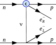
(c) The The nucleon-nucleon long-range $\mathcal{L}_{6}$ mode.

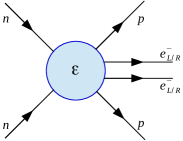
(d) The nucleon-nucleon short-range part of the $0\nu\beta\beta$ diagram.

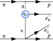
(e) The pion-neutrino long-range diagram.

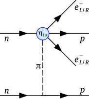
(f) The one-pion long-range diagram.

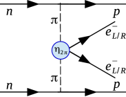
(g) The two-pion long-range diagram.

Figure 2: Similar to Fig.1, we present the nucleon-level diagrams of $0\nu\beta\beta$ decay process : (2a) presents the generic description of the process, (2b) shows the light left-handed neutrino exchange, (2c) is the long-range component, Subfigure 2d shows the short-range contribution. On the second line, (2e) is the pion-neutrino component, (2f) is the one-pion long-range contribution of the $\cancel{\cal{R}}_{p}$ SUSY induced $0\nu\beta\beta$ diagram, and (2g presents the two-pion long-range contribution of the $\cancel{\cal{R}}_{p}$ SUSY induced $0\nu\beta\beta$. The effective couplings $\eta_{1\pi}$ and $\eta_{2\pi}$ are related to Eq. (IV.3) as $\eta_{1\pi}=c_{1\pi}\eta_{\pi N}$ and $\eta_{2\pi}=c_{2\pi}\eta_{\pi N}$.

The contribution of the diagrams 1b and 1c to the $0\nu\beta\beta$ decay amplitude is proportional to the time-ordered product of two effective $\mathcal{L}_{6}$ Lagrangians Deppisch et al. (2012),

$$\!\!T(\mathcal{L}_{6}^{(1)}\mathcal{L}_{6}^{(2)}) =\frac{G^{2}_{F}}{2}T\left[j_{V-A}J^{\dagger}_{V-A}j_{V-A}J^{\dagger}_{V-A}\right.$$

$$+\left.\epsilon_{\alpha}^{\beta}j_{\beta}J^{\dagger}_{\alpha}j_{V-A}J^{\dagger}_{V-A}+\epsilon_{\alpha}^{\beta}\epsilon_{\gamma}^{\delta}j_{\beta}J^{\dagger}_{\alpha}j_{\delta}J^{\dagger}_{\gamma}\right],$$ (4)

while the contribution of the diagram 1d is proportional to $\mathcal{L}_{9}$.

However, when calculating the $0\nu\beta\beta$ half-life it is necessary to identify the contributions corresponding to different hadronization prescriptions. Figure 2 shows the nucleon-level diagrams in a similar way to Figure 1. The first 3 contributions, Figs. 2b, 2c, and 2d are similar to the corresponding amplitudes at the quark level (see Fig. 1). In addition to these contributions that were also considered in Ref. Deppisch et al. (2012), here we also include the long range diagrams that involve pion(s) exchange, Figs. 2e, 2f, and 2g. These diagrams were considered before as contributing to the $0\nu\beta\beta$ decay rate, but in the context of $\cancel{\cal{R}}_{p}$ SUSY mechanism. For example, the diagram 2e was considered to describe the contribution of the squark-exchange mechanism Faessler et al. (2008), and the diagrams 2f and 2g were considered to describe the contribution of the gluino exchange mechanism Wodecki et al. (1999). One should also mention that the diagram 2g was also considered in Refs. Prezeau et al. (2003); Peng et al. (2016), but its contribution to the $0\nu\beta\beta$ half-life was estimated differently, and cannot be directly compared to the other contributions analyzed here.

After hadronization (see Fig. 2), the extra terms in the Lagrangian require the knowledge of 23 individual NME Hirsch et al. (1996b); Deppisch et al. (2012); Pas et al. (1999, 2001); Deppisch et al. (2015); Vergados et al. (2012). We can write the half-life in a factorized compact form

$$\left[T^{0\nu}_{1/2}\right]^{-1}\!\!\!\!= g_{A}^{4}\left[\sum_{i}\left|\mathcal{E}_{i}\right|^{2}{\cal{M}}_{i}^{2}+\textnormal{Re}\left[\sum_{i\neq j}\mathcal{E}_{i}\mathcal{E}_{j}{\cal{M}}_{ij}\right]\right].$$ (5)

Here, the $\mathcal{E}_{i}$ contain the neutrino physics parameters, with $\mathcal{E}_{1}=\eta_{0\nu}$ representing the exchange of light left-handed neutrinos corresponding to Fig. 2b, $\mathcal{E}_{2-7}=\{\epsilon^{V+A}_{V-A},\ \epsilon^{V+A}_{V+A},\ \epsilon^{S+P}_{S\pm P},\ \epsilon^{TR}_{TL},\ \epsilon^{TR}_{TR},\ \eta_{\pi\nu}\}$ are the long-range LNV parameters appearing in Figs. 2c and 2e, and $\mathcal{E}_{8-15}=\{\varepsilon_{1},\ \varepsilon_{2},\ \varepsilon_{3}^{LLz(RRz)},\ \varepsilon_{3}^{LRz(RLz)},\ \varepsilon_{4},\ \varepsilon_{5},\ \eta_{1\pi},\ \eta_{2\pi}\}$ denote the short-range LNV parameters at the quark level involved in the diagrams of Fig. 2d, 2f, 2g. The rational for including the $\eta_{\pi\nu}$ in the same class with the LNV entering the quark-level long range diagrams is that Ref. Faessler et al. (2008) indicates that $\eta_{\pi\nu}$ is proportional to $\epsilon^{TR}_{TR}$ (see Section IV.2 below). In the same vein, Ref. Wodecki et al. (1999) indicates that $\varepsilon_{1}$ and $\varepsilon_{2}$ are proportional to a combination of $\eta_{1\pi}$ and $\eta_{2\pi}$ (see Section IV.3 below). Therefore the $\eta_{1\pi}$ and $\eta_{2\pi}$ were included in the list LNV couplings associated with quark-level short-range diagrams. Contributions of pion-exchange diagrams similar to those of Figs. 2f and 2g are also included in the so called ”higher order term in nucleon currents” Vergados et al. (2012). However, they are constrained by PCAC, and are only included in light-neutrino exchange contribution of diagram 2a. This contribution changes the associated NME by only 20%. Therefore, we conclude that this does not represent a serious double counting issue.

Following Refs. Pas et al. (1999, 2001); Deppisch et al. (2012); Vergados et al. (2012), we write ${\cal{M}}_{i}^{2}$ as combinations of NME described in Eqs. (8, 10, 12, 14, and IV.3) (see also Eq.(VII) in the Appendix for the individual NME) and integrated PSF Horoi and Neacsu (2016c) denoted with $G_{01}-G_{09}$. Our values of the PSF are presented in Table LABEL:tab-psf. In some cases the interference terms $\mathcal{E}_{i}\mathcal{E}_{j}{\cal{M}}_{ij}$ are small Ahmed et al. (2017) and can be neglected, but not all of them. In Ref. Horoi and Neacsu (2016a) we analyzed a subset of terms contributing to the half-life formula, Eq. (II) originating from the left-right symmetric model. In that restrictive case we showed that one can disentangle different contributions to the $0\nu\beta\beta$ decay process using two-electron angular and energy distributions as well as half-lives of two selected isotopes. Obviously, this number of observables is not enough to extract all coupling appearing in the effective field theory Lagrangian. However, they can be used to constrain these couplings, thus adding to the information extracted from the Large Hadron Collider and other related experiments. Here we attempt to extract these couplings assuming that only one of them can have a dominant contribution to the half-life, Eq. (5). We call this approach “on-axis“. Considering the “on-axis“ approach to extracting limits of the LNV parameters, the interference terms are neglected in our analysis. In the following, we extract the “on-axis“ upper limits of these parameters using the most recent experimental half-lives lower limits, as presented in Table LABEL:tab-psf.

IV Experimental limits on the BSM LNV couplings

To obtain experimentally constrained upper limits of the effective LNV couplings one needs experimental half-life lower limits, accurate calculations of the PSF, together with reliable NME results calculated using nuclear structure methods tested to correctly describe the experimental nuclear structure data available for the nuclei involved. We split our analysis of the LNV parameters into three subsections corresponding the exchange of light left-handed Majorana neutrinos, the LNV couplings entering the remaining quark-level long-range diagrams, and the LNV couplings entering the quark-level short-range diagrams.

IV.1 The exchange of light left-handed neutrinos

Most studies in the literature have considered just the case where only the exchange of light left-handed Majorana neutrinos contribute to the $0\nu\beta\beta$ decay process, presented in Figs. 1b and 2b. Therefore, one can easily find calculations of NME and PSF for this scenario. Considering this case, we reduce the half-life equation to:

$$\left[T^{0\nu}_{1/2}\right]^{-1}=g_{A}^{4}\left|\eta_{0\nu}\right|^{2}{\cal{M}}_{0\nu}^{2},$$ (6)

where $g_{A}=1.27$, ${\cal{M}}^{2}_{0\nu}$ contains the coefficients containing combinations of NME and PSF (see Eq. (8) below). $\eta_{0\nu}=\frac{\left<m_{\beta\beta}\right>}{m_{e}}$, where $m_{e}$ is the electron mass and ${\left<m_{\beta\beta}\right>}$ represents the effective Majorana neutrino mass described as Rodejohann (2012):

$$\left<m_{\beta\beta}\right>=\left|\sum_{j=1}^{3}U^{2}_{ej}m_{j}\right|.$$ (7)

Here $U_{ej}$ are the PMNS mixing matrix elements Maki et al. (1962); Beringer et al. (2012) and the summation is performed over all the three light neutrino mass eigenstates $m_{j}$. Also in Eq. (6)

$${\cal{M}}^{2}_{0\nu}=G_{01}\left[M_{GT}-\left(\frac{g_{V}}{g_{A}}\right)^{2}M_{F}+M_{T}\right]^{2},$$ (8)

where $g_{V}=1$ is the vector coupling constant, $g_{A}=1.27$ is the axial coupling constant, and $G_{01}$ is the phase-space factor. The three NME, $M_{GT}$, $M_{F}$, and $M_{T}$ (shown in Table LABEL:tab-nme-light) correspond to the Gamow-Teller, Fermi and Tensor transition operators, respectively, and are described in the Appendix. All the NME listed in the tables of the Appendix have the correct signs relative to that of $M_{GT}$, which is chosen to be positive. The ${\cal{M}}^{2}$ coefficients correctly include these relative signs, but the overall sign of the $\cal{M}$ in Eqs. (8, 10, 12, 14, and IV.3) is lost due to squaring.

Table 3: The first line shows values of the ${\cal{M}}_{0\nu}^{2}$ coefficients containing combinations of NME and PSF, and the second line presents the extracted neutrino physics parameter $\left|\eta_{0\nu}\right|$ for the most studied case, assuming only the exchange of light left-handed Majorana neutrinos.

		48Ca	76Ge	82Se	130Te	136Xe
${\cal{M}}_{0\nu}^{2}$	$\cdot 10^{14}$	$2.61$	$3.01$	$11.6$	$5.23$	$4.41$
$\left|\eta_{0\nu}\right|$	$\cdot 10^{6}$	$27.1$	$0.49$	$3.6$	$1.36$	$0.28$

In Table LABEL:tab-mrond-light we present the ${\cal{M}}_{0\nu}^{2}$ values and their corresponding $\eta_{0\nu}$ limits. We find the lowest upper-limit of this parameter for ¹³⁶Xe, which leads to a limit for the Majorana neutrino mass $\left<m_{\beta\beta}\right>\sim 140$ meV.

IV.2 The long-range effective LNV couplings

Investigating the “on-axis“ LNV parameters of the diagram of Fig. 2c, the half-life is factorized as:

$$\left[T^{0\nu}_{1/2}\right]^{-1}=g_{A}^{4}\left[\left|\epsilon_{\alpha}^{\beta}\right|^{2}{\cal{M}}_{\alpha\beta}^{2}\right],$$ (9)

with $\epsilon_{\alpha}^{\beta}=\{\epsilon^{V+A}_{V-A},\ \epsilon^{V+A}_{V+A},\ \epsilon^{S+P}_{S\pm P},\ \epsilon^{TR}_{TL},\ \epsilon^{TR}_{TR}\}$. Here and below the $\alpha\beta$ combination corresponds to some index $i$ in Eq. (5), as described in the definition of $\mathcal{E}_{i}$ after Eq. (5). Following the formalism presented in Refs. Deppisch et al. (2012); Pas et al. (1999); Doi et al. (1985) and including the $G_{01}-G_{09}$ PSF, we write the long-range coefficients containing combinations of NME and PSF as:

$${\cal{M}}_{V+A/V-A}^{2} =G_{02}{\cal{M}}^{2}_{2+}\!\!-\frac{2}{9}G_{03}{\cal{M}}_{1-}{\cal{M}}_{2+}\!\!+\frac{1}{9}G_{04}{\cal{M}}^{2}_{1-}$$

$$-G_{07}M_{P}M_{R}+G_{08}M^{2}_{P}+G_{09}M^{2}_{R},$$ (10a)

$${\cal{M}}_{V+A/V+A}^{2} =G_{02}{\cal{M}}^{2}_{2-}$$

$$-\frac{2}{9}G_{03}{\cal{M}}_{1+}{\cal{M}}_{2-}+\frac{1}{9}G_{04}{\cal{M}}^{2}_{1+},$$ (10b)

$${\textmd{with\ }}{\cal{M}}_{1\pm} =M_{GTq}\pm 3\left(\frac{g_{V}}{g_{A}}\right)^{2}M_{Fq}-6M_{Tq}$$

$${\textmd{and}}\ {\cal{M}}_{2\pm} =M_{GT\omega}\pm\left(\frac{g_{V}}{g_{A}}\right)^{2}M_{F\omega}-\frac{1}{9}{\cal{M}}_{1\pm},$$

$${\cal{M}}_{S+P/S\pm P}^{2} =G_{01}\left[\frac{F^{(3)}_{P}}{Rm_{e}g_{A}}\left(\frac{1}{3}M_{GT^{\prime}}+M_{T^{\prime}}\right)\right]^{2}\!\!\!\!,$$ (10c)

$${\cal{M}}_{TR/TR}^{2} =G_{01}\left[\frac{4T^{(3)}_{1}g_{V}(1-(\mu_{p}-\mu_{n}))}{Rm_{e}g_{A}^{2}}\right.$$

$$\times\left.\left(M_{T^{\prime}}-\frac{2}{3}M_{GT^{\prime}}\right)\right]^{2},$$ (10d)

$${\cal{M}}_{TR/TL}^{2} =G_{01}\left[\frac{g_{V}\left(8\hat{T}^{(3)}_{2}-4T^{(3)}_{1}\right)}{Rm_{e}g_{A}^{2}}M_{F^{\prime}}\right.$$

$$-\left.\frac{4T_{1}^{(3)}2m_{p}}{g_{A}R^{2}m_{e}m^{2}_{\pi}}\left(M_{T^{\prime\prime}}+\frac{1}{3}M_{GT^{\prime\prime}}\right)\right]^{2}\!\!\!\!.$$ (10e)

In these equations, $R=1.2A^{1/3}$ fm is the nuclear radius, $m_{e}=0.511$ MeV is the electron mass, $m_{\pi}=139$ MeV is the pion mass, $m_{p}=938$ MeV is the proton mass, $(\mu_{p}-\mu_{n})\simeq 3.7$, and the parameters $F_{P}^{(3)}=4.41$, $T_{1}^{(3)}=1.38$, $\hat{T}_{2}^{(3)}=-4.54$ are taken from Ref. Adler et al. (1975) where they have been calculated using the MIT bag model. Detailed expressions for the individual $M_{\alpha}$ (with $\alpha=$ $GTq$, $Fq$, $Tq$, $GT\omega$, $F\omega$, $P$, $R$, $GT^{\prime}$, $F^{\prime}$, $T^{\prime}$, $GT^{\prime\prime}$, $T^{\prime\prime}$) are found in the Appendix.

It is possible to obtain another limit for $\epsilon_{TR}^{TR}$ by considering a different hadronization procedure Faessler et al. (2008) depicted in Fig. 2e, where our $\eta_{\pi\nu}$ plays the same role as $\eta^{11}_{(q)LR}$ in Eq.(22) of Ref. Faessler et al. (2008). In this case we can obtain an alternative value for $\epsilon_{TR}^{TR}$, $\tilde{\epsilon}_{TR}^{TR}=\eta_{\pi\nu}/8$.

$$\left[T^{0\nu}_{1/2}\right]^{-1}=g_{A}^{4}\left[\left|8\ \tilde{\epsilon}_{TR}^{TR}\right|^{2}{\cal{M}}_{\pi\nu}^{2}\right],$$ (11)

with

$${\cal{M}}_{\pi\nu}^{2}=G_{01}\left[M_{GT{\pi\nu}}+M_{T{\pi\nu}}\right]^{2}.$$ (12)

The $M_{GT{\pi\nu}}$ and $M_{T{\pi\nu}}$ are the same NME as $M_{GT(\tilde{q})}$ and $M_{GT(\tilde{q})}$ in Eq.(155) of Ref.Vergados et al. (2012) (also described in the Appendix).

Table 4: The ${\cal{M}}_{\alpha\beta}^{2}$ values for the long-range part of the $0\nu\beta\beta$ decay process.

		48Ca	76Ge	82Se	130Te	136Xe
$10^{9}\cdot$	${\cal{M}}_{V+A/V-A}^{2}$	$1.49$	$1.44$	$5.24$	$3.76$	$3.17$
$10^{13}\cdot$	${\cal{M}}_{V+A/V+A}^{2}$	$1.09$	$0.39$	$3.21$	$1.11$	$0.89$
$10^{10}\cdot$	${\cal{M}}_{S+P/S\pm P}^{2}$	$1.62$	$1.17$	$4.20$	$4.73$	$4.18$
$10^{8}\cdot$	${\cal{M}}_{TR/TR}^{2}$	$6.07$	$1.15$	$4.43$	$2.45$	$1.95$
$10^{7}\cdot$	${\cal{M}}_{TR/TL}^{2}$	$3.42$	$0.25$	$0.80$	$1.74$	$1.59$
$10^{10}\cdot$	${\cal{M}}_{\pi\nu}^{2}$	$2.84$	$2.62$	$10.2$	$4.85$	$4.13$

Table LABEL:tab-mrond-lr shows our shell model ${\cal{M}}^{2}_{\alpha\beta}$ coefficients. We present our values for the long-range LNV parameters in Table LABEL:tab-epslr, where $\tilde{\epsilon}^{TR}_{TR}$ represents the alternative limit for $\epsilon^{TR}_{TR}$ that is obtained using ${\cal{M}}_{\pi\nu}$. With the exception of ⁴⁸Ca, the $\tilde{\epsilon}^{TR}_{TR}$ upper-limits are slightly lower than those of $\epsilon^{TR}_{TR}$.

Table 5: The “on-axis“ values of the long-range LNV parameters $\epsilon^{\beta}_{\alpha}$. The last two lines present $\eta_{\pi\nu}$ and its corresponding $\tilde{\epsilon}^{TR}_{TR}$ limit.

	48Ca	76Ge	82Se	130Te	136Xe
$\left|\epsilon^{V+A}_{V-A}\right|$	$1.1\cdot 10^{-7}$	$2.2\cdot 10^{-9}$	$1.7\cdot 10^{-8}$	$5.1\cdot 10^{-9}$	$1.1\cdot 10^{-9}$
$\left|\epsilon^{V+A}_{V+A}\right|$	$1.3\cdot 10^{-5}$	$4.3\cdot 10^{-7}$	$2.2\cdot 10^{-6}$	$9.3\cdot 10^{-7}$	$2.0\cdot 10^{-7}$
$\left|\epsilon^{S+P}_{S\pm P}\right|$	$3.4\cdot 10^{-7}$	$7.9\cdot 10^{-9}$	$6.1\cdot 10^{-8}$	$1.4\cdot 10^{-8}$	$2.9\cdot 10^{-9}$
$\left|\epsilon^{TR}_{TR}\right|$	$1.8\cdot 10^{-8}$	$7.9\cdot 10^{-10}$	$5.9\cdot 10^{-9}$	$2.0\cdot 10^{-9}$	$4.2\cdot 10^{-10}$
$\left|\epsilon^{TR}_{TL}\right|$	$7.5\cdot 10^{-9}$	$5.4\cdot 10^{-10}$	$4.4\cdot 10^{-9}$	$7.4\cdot 10^{-10}$	$1.5\cdot 10^{-10}$
$\left|\eta_{\pi\nu}\right|$	$2.6\cdot 10^{-7}$	$5.3\cdot 10^{-9}$	$3.9\cdot 10^{-8}$	$1.4\cdot 10^{-8}$	$2.9\cdot 10^{-9}$
$\left|\tilde{\epsilon}^{TR}_{TR}\right|$	$3.3\cdot 10^{-8}$	$6.6\cdot 10^{-10}$	$4.8\cdot 10^{-9}$	$1.8\cdot 10^{-9}$	$3.6\cdot 10^{-10}$

The shell model values for $M_{\alpha}$, with $\alpha=$ $GTq$, $Fq$, $Tq$, $GT\omega$, $F\omega$, $P$, $R$, $GT^{\prime}$, $F^{\prime}$, $T^{\prime}$, $GT^{\prime\prime}$, $T^{\prime\prime}$, $GT\pi\nu$, $T\pi\nu$, are shown in Table LABEL:tab-nme-muto of the Appendix.

IV.3 The short-range LNV couplings

Similar to the case of the long-range component, we extract the “on-axis“ values of the short-range LNV parameters using the following expression for the half-life corresponding to the diagram of Fig. 1d:

$$\left[T^{0\nu}_{1/2}\right]^{-1}=g_{A}^{4}\left[\left|\varepsilon_{\alpha}^{\beta}\right|^{2}{\cal{M}}_{\alpha\beta}^{2}\right],$$ (13)

with $\varepsilon_{\alpha}^{\beta}=\{\varepsilon_{1},\ \varepsilon_{2},\ \varepsilon_{3}^{LLz(RRz)},\ \varepsilon_{3}^{LRz(RLz)},\ \varepsilon_{4},\ \varepsilon_{6}\}$. The index $\beta=xyz$, with $xyz=L/R,L/R,L/R$, indicates the chirality of the hadronic and the leptonic currents. It is only possible to distinguish between the different chiralities in the case of $\varepsilon_{3}$ where we denote them explicitly as $\varepsilon_{3}^{LLz(RRz)}$ and $\varepsilon_{3}^{LRz(RLz)}$. For the other cases we omit this labeling.

Adapting the formalism of Ref. Deppisch et al. (2012); Pas et al. (2001); Vergados et al. (2012), we can write the coefficients containing combinations of NME and PSF as:

$${\cal{M}}_{1}^{2} =G_{01}\left[\left(\frac{F_{S}^{(3)}}{g_{A}}\right)^{2}M_{FN}\right]^{2},$$ (14a)

$${\cal{M}}_{2}^{2} =G_{01}\left[\left(8\frac{T_{1}^{(3)}}{g_{A}}\right)^{2}M_{GTN}\right]^{2},$$ (14b)

$${\cal{M}}_{3LLz}^{2} ={\cal{M}}_{3RRz}^{2}$$

$$=G_{01}\left[M_{GTN}-\left(\frac{g_{V}}{g_{A}}\right)^{2}M_{FN}\right]^{2},$$ (14c)

$${\cal{M}}_{3LRz}^{2} ={\cal{M}}_{3RLz}^{2}$$

$$=G_{01}\left[M_{GTN}+\left(\frac{g_{V}}{g_{A}}\right)^{2}M_{FN}\right]^{2},$$ (14d)

$${\cal{M}}_{4}^{2} =G_{09}\frac{\left(m_{e}R\right)^{2}}{8}\left[\frac{T_{1}^{(3)}}{g_{A}}M_{GTN}\right]^{2},$$ (14e)

$${\cal{M}}_{5}^{2} =G_{09}\frac{\left(m_{e}R\right)^{2}}{8}\left[\frac{F_{S}^{(3)}g_{V}}{g_{A}^{2}}M_{FN}\right]^{2}.$$ (14f)

The parameters $F_{S}^{(3)}=0.48$ and $T_{1}^{(3)}=1.38$ are taken form Ref. Adler et al. (1975). The values of these ${\cal{M}}_{\alpha\beta}^{2}$ are presented in Table LABEL:tab-mrond-sr. Detailed expressions for $M_{GTN}$ and $M_{FN}$ are presented in the Appendix, and their shell model values are shown in Table LABEL:tab-heavy.

Considering the $0\nu\beta\beta$ amplitudes displayed in Figs. 2f and 2g in the one-pion and two-pion exchange modes it is possible to get alternative limits for $\varepsilon_{1}$ and $\varepsilon_{2}$ considering a different coefficient, ${\cal{M}}_{\pi N}$. The analysis of Ref. Wodecki et al. (1999) suggests these alternative values, here denoted by $\tilde{\varepsilon}_{1}$ and $\tilde{\varepsilon}_{2}$, can be obtained as $\tilde{\varepsilon}_{1}=\frac{64}{16}\eta_{\pi N}$, and $\tilde{\varepsilon}_{2}=\frac{2}{3}\eta_{\pi N}$, using

$$\left[T^{0\nu}_{1/2}\right]^{-1}=g_{A}^{4}\left[\left|\eta_{\pi N}\right|^{2}{\cal{M}}_{\pi N}^{2}\right],$$ (15)

where

$${\cal{M}}_{\pi N}^{2} =G_{01}\left[c^{1\pi}\left(M_{GT1\pi}+M_{T1\pi}\right)\right.$$

$$+\left.c^{2\pi}\left(M_{GT2\pi}+M_{T2\pi}\right)\right]^{2}.$$ (16)

The expressions for the factors $c^{1\pi}$ and $c^{2\pi}$ are found in Eq. (151) of Ref. Vergados et al. (2012). These factors depend on the masses of the up and down quark, and choosing $(m_{u}+m_{d})=11.6$ MeV Faessler et al. (1998); Horoi (2013), one gets $c^{1\pi}=-83.598$, $c^{2\pi}=359.436$ that we use in these calculations. The description of $M_{\alpha}$ (with $\alpha=GT1\pi,\ T1\pi,\ GT2\pi,\ T2\pi$) is presented in the Appendix.

Table 6: The ${\cal{M}}_{\alpha\beta}^{2}$ values for the short-range LNV parameters.

		48Ca	76Ge	82Se	130Te	136Xe
$10^{13}\cdot$	${\cal{M}}_{1}^{2}$	$2.63$	$1.83$	$6.86$	$4.83$	$4.03$
$10^{8}\cdot$	${\cal{M}}_{2}^{2}$	$0.75$	$0.54$	$2.00$	$1.46$	$1.21$
$10^{10}\cdot$	${\cal{M}}_{3LLz(RRz)}^{2}$	$1.30$	$0.92$	$3.45$	$2.50$	$2.07$
$10^{11}\cdot$	${\cal{M}}_{3LRz(RLz)}^{2}$	$4.82$	$3.48$	$13.0$	$9.54$	$7.87$
$10^{10}\cdot$	${\cal{M}}_{4}^{2}$	$1.00$	$0.75$	$2.68$	$1.89$	$1.56$
$10^{12}\cdot$	${\cal{M}}_{5}^{2}$	$1.15$	$0.84$	$3.01$	$2.06$	$1.72$
$10^{9}\cdot$	${\cal{M}}_{\pi N}^{2}$	$3.36$	$0.87$	$3.24$	$2.43$	$1.94$

Shown in Table LABEL:tab-epssr are the values of the short-range LNV parameters. Using the different hadronization presented in Figs. 2f and 2g, $\tilde{\varepsilon}_{1}$ provides significantly more stringent upper-limits than $\varepsilon_{1}$. With the exception of ⁴⁸Ca, where the $\tilde{\varepsilon}_{2}$ limit is identical to $\varepsilon_{2}$, the other $\tilde{\varepsilon}_{2}$ upper-limits are almost double those of $\varepsilon_{2}$. Therefore, we conclude that $\varepsilon_{2}$ are better constrained.

Table 7: The “on-axis“ values of the short-range LNV parameters $\varepsilon^{\beta}_{\alpha}$. The last three lines present the $\eta_{\pi N}$ limits for $\cancel{\cal{R}}_{p}$ SUSY, and their corresponding $\tilde{\varepsilon}_{1}$ and $\tilde{\varepsilon}_{1}$ limits, respectively.

	48Ca	76Ge	82Se	130Te	136Xe
$|\varepsilon_{1}|$	$8.6\cdot 10^{-6}$	$2.0\cdot 10^{-7}$	$1.5\cdot 10^{-6}$	$4.5\cdot 10^{-7}$	$9.3\cdot 10^{-8}$
$|\varepsilon_{2}|$	$5.1\cdot 10^{-8}$	$1.2\cdot 10^{-9}$	$8.8\cdot 10^{-9}$	$2.6\cdot 10^{-9}$	$5.4\cdot 10^{-10}$
$|\varepsilon_{3}^{LLz(RRz)}|$	$3.8\cdot 10^{-7}$	$8.9\cdot 10^{-9}$	$6.7\cdot 10^{-8}$	$2.0\cdot 10^{-8}$	$4.1\cdot 10^{-9}$
$|\varepsilon_{3}^{LRz(RLz)}|$	$6.3\cdot 10^{-7}$	$1.4\cdot 10^{-8}$	$1.1\cdot 10^{-7}$	$3.2\cdot 10^{-8}$	$6.7\cdot 10^{-9}$
$|\varepsilon_{4}|$	$4.4\cdot 10^{-7}$	$9.8\cdot 10^{-9}$	$7.6\cdot 10^{-8}$	$2.3\cdot 10^{-8}$	$4.7\cdot 10^{-9}$
$|\varepsilon_{5}|$	$4.1\cdot 10^{-6}$	$9.3\cdot 10^{-8}$	$7.1\cdot 10^{-7}$	$2.2\cdot 10^{-7}$	$4.5\cdot 10^{-8}$
$|\eta_{\pi N}|$	$7.6\cdot 10^{-8}$	$2.9\cdot 10^{-9}$	$2.2\cdot 10^{-8}$	$6.3\cdot 10^{-9}$	$1.3\cdot 10^{-9}$
$|\tilde{\varepsilon}_{1}|$	$3.2\cdot 10^{-7}$	$1.2\cdot 10^{-8}$	$9.3\cdot 10^{-8}$	$2.7\cdot 10^{-8}$	$5.7\cdot 10^{-9}$
$|\tilde{\varepsilon}_{2}|$	$5.0\cdot 10^{-8}$	$1.9\cdot 10^{-9}$	$1.5\cdot 10^{-8}$	$4.2\cdot 10^{-9}$	$8.9\cdot 10^{-10}$

V Discussions

From the $\eta_{0\nu}$ limits presented in Table LABEL:tab-mrond-light for ¹³⁶Xe, one gets the lowest shell model upper-limit for the Majorana neutrino mass $\left<m_{\beta\beta}\right>\sim 140$ meV. A wider range of values, $60-165$ meV can be found if the NME calculated with a larger number of nuclear models are considered Gando et al. (2016).

Considering the diagram in Fig. 2e, it is possible to get lower limits for $\epsilon^{TR}_{TR}$, denoted as $\tilde{\epsilon}^{TR}_{TR}$ in Table LABEL:tab-epslr, than those corresponding to the diagram in Fig. 2c, with the exception of ⁴⁸Ca, as can be seen in Table LABEL:tab-epslr. Considering the different hadronization scenario presented in Figs. 2f and 2g, $\tilde{\varepsilon}_{1}$ provides a significantly more stringent upper-limits than $\varepsilon_{1}$. With the exception of ⁴⁸Ca, where the $\tilde{\varepsilon}_{2}$ limit is identical to $\varepsilon_{2}$, the other $\tilde{\varepsilon}_{2}$ upper-limits are almost double those of $\varepsilon_{2}$.

Table 8: The BSM effective scale (in GeV) for different dimension-D operators at the present ¹³⁶Xe half-life limit ($\Lambda^{0}_{D}$) and for $T_{1/2}\approx 1.1\times 10^{28}$ years ($\Lambda_{D}$).

${\cal{O}}_{D}$	$\ \ \bar{\epsilon}_{D}$	$\ \ \Lambda^{0}_{D}(y=1)$	$\ \ \Lambda^{0}_{D}(y=y_{e})$	$\ \ \Lambda_{D}(y=y_{e})$
${\cal{O}}_{5}$	$\ \ 2.8\cdot 10^{-7}$	$\ \ 2.12\cdot 10^{14}$	1904	19044
${\cal{O}}_{7}$	$\ 2.0\cdot 10^{-7}$	$\ \ 3.76\cdot 10^{4\ }$	542	1169
${\cal{O}}_{9}$	$\ \ 9.3\cdot 10^{-8}$	$\ \ 2.72\cdot 10^{3\ }$	2718	4307
${\cal{O}}_{11}$	$\ \ 9.3\cdot 10^{-8}$	$\ \ 1.24\cdot 10^{3\ }$	33	46

As suggested in Ref. Deppisch et al. (2015) (see the diagrams of their Fig.1), at the electroweak scale when the appropriate Higgs fields are included, the diagram 1.b originates from a dimension-5 BSM Lagrangian, $\mathcal{O}_{5}$, responsible for the Majorana neutrino mass. Similarly the low-energy dimension-6 Lagrangian $\mathcal{L}_{6}$ corresponds to a dimension-7 BSM operator, $\mathcal{O}_{7}$, and the low energy dimension-9 Lagrangian $\mathcal{L}_{9}$ can be rearranged as dimension-9 and dimension-11 operators, $\mathcal{O}_{9}$ and $\mathcal{O}_{11}$. Using the effective field theory one can infer the energy scale $\Lambda_{D}$ up to which these effective field operators are not broken:

$$\mathcal{L}_{D}=\frac{g}{\left(\Lambda_{D}\right)^{D-4}}\mathcal{O}_{D},$$ (17)

where $D$ is the dimension of the effective field operator. Here $g$ is considered to be a dimensionless coupling constant of the order of 1. Following Ref. Deppisch et al. (2015) one can find relations between the constants entering our $\mathcal{L}_{6}$ and $\mathcal{L}_{9}$ Lagrangian and the effective field theory Lagrangians above the electroweak scale, Eq. (17).

$$m_{e}\bar{\epsilon}_{5}=\frac{g^{2}(yv)^{2}}{\Lambda_{5}}, \frac{G_{F}\bar{\epsilon}_{7}}{\sqrt{2}}=\frac{g^{3}(yv)}{2(\Lambda_{7})^{3}},$$

$$\frac{G^{2}_{F}\bar{\epsilon}_{9}}{2m_{p}}=\frac{g^{4}}{(\Lambda_{9})^{5}}, \frac{G^{2}_{F}\bar{\epsilon}_{11}}{2m_{p}}=\frac{g^{6}(yv)^{2}}{(\Lambda_{11})^{7}}.$$ (18)

Here, $m_{e}=0.511\times 10^{-3}$ GeV is the electron mass, $g=1$ is a generic coupling constant, $v=174$ GeV is the Higgs vacuum expectation value, $y$ is a Yukawa coupling associated to the interaction with the Higgs bosons, $G_{F}=1.166\times 10^{-5}$ GeV^-2 is the Fermi coupling constant, and $m_{p}=0.938$ GeV is the proton mass. The $\bar{\epsilon}_{D}$ (with $D=\{5,\ 7,\ 9,\ 11\}$) can be extracted from the LNV parameters in Eqs. (2) and (3). Considering that values of these LNV parameters may be affected by mixing angles that might distort the scales in Eq. (17), we choose their maximum values: $\bar{\epsilon}_{5}=|\eta_{0\nu}|$, $\bar{\epsilon}_{7}=\textmd{Max}\Bigl{[}|\epsilon^{V+A}_{V-A}|\Bigr{.}$, $|\epsilon^{V+A}_{V+A}|$, $|\epsilon^{S+P}_{S\pm P}|$, $|\epsilon^{TR}_{TL}|$, $\Bigl{.}|\epsilon^{TR}_{TR}|\Bigr{]}$, $\bar{\epsilon}_{9}=\textmd{Max}\Bigl{[}|\varepsilon_{1}|\Bigr{.}$, $|\varepsilon_{2}|$, $|\varepsilon_{3}^{LLz(RRz)}|$, $|\varepsilon_{3}^{LRz(RLz)}|$, $|\varepsilon_{4}|$, $\Bigl{.}|\varepsilon_{5}|\Bigr{]}$, and $\bar{\epsilon}_{11}=\bar{\epsilon}_{9}$.

To extract the limits of the BSM scales $\Lambda_{5,7,9,11}$ we need the most stringent limits for the LNV parameters, which are found for the case of ¹³⁶Xe. Inspecting Tables LABEL:tab-epslr and LABEL:tab-epssr we found that $\bar{\epsilon}_{5}$ corresponds to the $\eta_{0\nu}$ parameter of the light left-handed Majorana neutrino exchange mechanism. For $\bar{\epsilon}_{7}$ we choose $\epsilon^{V+A}_{V+A}$, that is the largest long-range $\epsilon_{\alpha}^{\beta}$ parameter. In the case of $\bar{\epsilon}_{9}=\bar{\epsilon}_{11}$ we select $\varepsilon_{1}$, being the largest short-range $\varepsilon_{\alpha}^{\beta}$ parameter. These values are listed in Table 8.

As in Ref. Deppisch et al. (2015) we take $g=1$ in Eq. (17). However, we introduce here the Yukawa coupling $y$ between the Higgs boson field and the fermion fields, and we consider two cases: (i) $y=1$ corresponding to the top quark mass (choice made in Ref. Deppisch et al. (2015)), and (ii) $y=3\times 10^{-6}$ corresponding to the electron mass. Based on these values we calculate the limits of the new BSM scales or different dimension-D operators. The results are shown in Table 8. The $\Lambda^{0}_{D}$ scales are calculated using the present lower limit for the half-life of ¹³⁶Xe, $1.1\times 10^{26}$. $\Lambda_{D}$ is estimated assuming a half-life of $T_{1/2}\approx 1.1\times 10^{28}$ years, which would correspond to a $\left<m_{\beta\beta}\right>\approx 14$ meV.

The $\Lambda_{9}$ scale does not depend on the unknown Yukawa coupling, and from that point of view, if $\mathcal{O}_{9}$ amplitude is dominant, that would indicate that the scale of new physics should be found around 3 TeV. Unfortunately, the $\Lambda_{9}$ scale, as well as all other high $D$ scales, are not very sensitive to the $0\nu\beta\beta$ half-life, because they scale as $T_{1/2}^{\frac{1}{2(D-4)}}$. $\mathcal{O}_{7}$ and $\mathcal{O}_{11}$ provide small low-limits for $\Lambda_{7}$ and $\Lambda_{11}$. This feature is likely related to the fact that these terms are originating from small term in the mixing matrix (e.g. the small $S$ matrix in Eq. (A3) of Horoi and Neacsu (2016a)), and thus $g\sim 1$ in Eq. (17) is not a good choice. The most sensitive scale to both the unknown Yukawa and the $0\nu\beta\beta$ half-life is $\Lambda_{5}$. Assuming a Yukawa coupling corresponding to the electron mass, one can conclude that the $0\nu\beta\beta$ decay could be consistent with a new physics scale somewhere between 2 TeV and 20 TeV.

VI Conclusions

This work advances and extends the analysis of BSM physics parameters involved in the neutrinoless double-beta decay. We calculate 23 nuclear matrix elements and 9 phase-space factors. Five of these nuclear matrix elements ($M_{GT^{\prime}}$, $M_{GT^{\prime\prime}}$, $M_{F^{\prime}}$, $M_{T^{\prime}}$, and $M_{T^{\prime\prime}}$) are calculated for the first time using shell model techniques. Three new hadron-level diagrams, Fig. 2.e, 2.f, 2.g are for the first time considered in the full analyses based on the effective field theory approach to $0\nu\beta\beta$ decay (they were only considered in the past in the context of particular mechanisms).

Using a general effective field theory and assuming that one LNV coupling plays a dominant contribution to the $0\nu\beta\beta$ decay amplitude, we extract limits for the effective Majorana mass and 11 effective low-energy couplings in the case of five nuclei of immediate experimental interest. Due to the better half-life limits, the most stringent limits for the LNV couplings are found for ¹³⁶Xe, closely followed by ⁷⁶Ge. An upper-limit for the Majorana neutrino mass $\left<m_{\beta\beta}\right>$ of 140 meV was calculated in the case of ¹³⁶Xe. Assuming a Yukawa coupling corresponding to the electron mass, one can conclude that the $0\nu\beta\beta$ decay could be consistent with a new physics scale somewhere between 2 TeV and 20 TeV.

Using the upper limits for the LNV coupling we extract limits for the energy scale of the new physics, using EFT arguments. We found that the scale associated with the dimension-9 EFT operator is stable, and indicates a new physics scale around 3 TeV. We also found that the dimension-5 EFT operator associated with the Majorana neutrino mass varies significantly with the Yukawa coupling to Higgs and the $0\nu\beta\beta$ decay half-life.

Should neutrinoless double-beta decay be experimentally observed, a thorough analysis of the outgoing electrons angular and energy distributions (presented in Ref. Horoi and Neacsu (2016a)) based on accurate calculations of the nuclear matrix elements is needed to investigate subsets of these LNV couplings and identify the presence of the right-handed currents.

VII Appendix

In this Appendix, we present the detailed expressions for the ${\cal{M}}_{i}^{2}$ coefficients that are needed to analyze the outcome of Eq.  (5).

The NME that enter the equations (8, 10, 12, 14, and IV.3) are written as a product of two-body transition densities (TBTD) and two-body matrix elements (TBME), where the summation is over all the nucleon states. Their numerical values when calculated within the shell model approach are presented in Table LABEL:tab-nme-light for the light left-handed Majorana neutrino exchange, in Table LABEL:tab-nme-muto for the long-range part in Fig. 2, and in Table LABEL:tab-heavy for the short-range component of Fig. 2. The general expressions for the NME are (see Refs. Doi et al. (1985); Horoi (2013); Horoi and Neacsu (2016a)):

$$M_{\alpha} =\sum_{j_{p}j_{p^{\prime}}j_{n}j_{n^{\prime}}J^{\pi}}TBTD\left(j_{p}j_{p^{\prime}},j_{n}j_{n^{\prime}};J^{\pi}\right)$$

$$\times\left<j_{p}j_{p^{\prime}};J^{\pi}\left\|\tau_{-1}\tau_{-2}{\cal{O}}^{\gamma,\phi,\theta,P,R}_{12}\right\|j_{n}j_{n^{\prime}};J^{\pi}\right>.$$ (19)

We group the operators that share similar structure into five families.

$$\textmd{Gamow-Teller operator}:{\cal{O}}^{\gamma}_{12}=\vec{\mkern 0.0mu\sigma}_{1}\cdot\vec{\mkern 0.0mu\sigma}_{2}H_{\gamma}(r),$$

$$\textmd{Fermi operator}:{\cal{O}}^{\phi}_{12}\ =H_{\phi}(r),$$

$$\textmd{Tensor operator}:{\cal{O}}^{\theta}_{12}=\left[3(\vec{\mkern 0.0mu\sigma}_{1}\cdot{\bf\hat{r}})(\vec{\mkern 0.0mu\sigma}_{2}\cdot{\bf\hat{r}})-\vec{\mkern 0.0mu\sigma}_{1}\cdot\vec{\mkern 0.0mu\sigma}_{2}\right]H_{\theta}(r),$$

$$\textmd{P operator}:{\cal{O}}^{P}_{12}=\left(\vec{\mkern 0.0mu\sigma}_{1}-\vec{\mkern 0.0mu\sigma}_{2}\right)H_{P}(r),$$

$$\textmd{R operator}:{\cal{O}}^{R}_{12}=\vec{\mkern 0.0mu\sigma}_{1}\cdot\vec{\mkern 0.0mu\sigma}_{2}H_{R}(r).$$

Here, $\gamma=$ $GT$, $GT\omega$, $GTq$, $GTN$, $GT^{\prime}$, $GT^{\prime\prime}$, $GT\pi\nu$, $GT1\pi$, $GT2\pi$, $\phi=F,\ F\omega,\ Fq,\ FN,\ F^{\prime}$, and $\theta=T,\ Tq,\ T^{\prime},\ T^{\prime\prime},\ T\pi\nu,\ T1\pi,\ T2\pi$. Equations (20) present the radial part of the NME and their expressions are adapted for consistency from Refs. Doi et al. (1985),Deppisch et al. (2012), and Vergados et al. (2012).

Table 9: NME values for the exchange of light left-handed Majorana neutrinos corresponding to the diagram in Fig. 2b.

	48Ca	76Ge	82Se	130Te	136Xe
$M_{GT}$	$0.807$	$3.206$	$3.005$	$1.662$	$1.505$
$M_{F}$	$-0.233$	$-0.674$	$-0.632$	$-0.438$	$-0.400$
$M_{T}$	$0.080$	$0.011$	$0.012$	$-0.007$	$-0.008$

Table 10: NME for the long-range part shown in Figs. 2c and 2e.

	48Ca	76Ge	82Se	130Te	136Xe
$M_{GTq}$	$0.709$	$3.228$	$3.034$	$1.587$	$1.440$
$M_{GT\omega}$	$0.930$	$3.501$	$3.287$	$1.855$	$1.682$
$M_{GT^{\prime}}$	$0.841$	$2.699$	$2.567$	$2.120$	$1.935$
$M_{GT^{\prime\prime}}$	$3.581$	$11.982$	$11.490$	$12.210$	$11.202$
$M_{GT\pi\nu}$	$86.2$	$331.6$	$313.3$	$184.2$	$167.7$
$M_{Fq}$	$-0.121$	$-0.383$	$-0.362$	$-0.249$	$-0.230$
$M_{F\omega}$	$-0.232$	$-0.659$	$-0.618$	$-0.427$	$-0.391$
$M_{F^{\prime}}$	$-0.258$	$-0.812$	$-0.772$	$-0.635$	$-0.581$
$M_{Tq}$	$-0.173$	$-0.059$	$-0.058$	$-0.013$	$-0.012$
$M_{T^{\prime}}$	$0.337$	$0.015$	$0.025$	$-0.077$	$-0.085$
$M_{T^{\prime\prime}}$	$2.231$	$0.028$	$0.118$	$-0.773$	$-0.861$
$M_{T\pi\nu}$	$21.3$	$7.3$	$6.9$	$1.2$	$1.1$
$M_{P}$	$0.395$	$-2.466$	$-2.332$	$-1.729$	$-1.617$
$M_{R}$	$1.014$	$3.284$	$3.127$	$2.562$	$2.341$

Table 11: The short-range NME involved in Figs. 2d, 2f, and 2g.

	48Ca	76Ge	82Se	130Te	136Xe
$M_{GTN}$	$58.5$	$162.3$	$150.1$	$107.6$	$96.6$
$M_{GT1\pi}$	$-1.354$	$-3.559$	$-3.282$	$-2.421$	$-2.171$
$M_{GT2\pi}$	$-0.676$	$-1.983$	$-1.854$	$-1.257$	$-1.136$
$M_{FN}$	$-22.9$	$-62.6$	$-58.1$	$-41.0$	$-36.9$
$M_{T1\pi}$	$-0.590$	$-0.010$	$-0.027$	$0.106$	$0.115$
$M_{T2\pi}$	$-0.227$	$-0.010$	$-0.015$	$0.038$	$0.040$

$$H_{GT} =\frac{2R}{\pi}\int\frac{h^{2}_{GT}(q^{2})}{q(q+\bar{E})}j_{0}(qr)q^{2}\differential{q},$$ (20a)

$$H_{GT\omega} =\frac{2R}{\pi}\int\frac{h_{A}^{2}(q^{2})}{(q+\bar{E})^{2}}j_{0}(qr)q^{2}\differential{q},$$ (20b)

$$H_{GTq} =\frac{2R}{\pi}r\int\frac{h_{A}^{2}(q^{2})}{q+\bar{E}}j_{1}(qr)q^{2}\differential{q},$$ (20c)

$$H_{GTN} =\frac{2R}{\pi m_{e}m_{p}}\int h_{A}^{2}(q^{2})j_{0}(qr)q^{2}\differential{q},$$ (20d)

$$H_{GT^{\prime}} =\frac{2R^{2}}{\pi m_{p}}\int\frac{q^{2}h_{A}^{2}(q^{2})}{q(q+\bar{E})}j_{0}(qr)q^{2}\differential{q},$$ (20e)

$$H_{GT^{\prime\prime}} =\frac{2R^{3}}{\pi m_{p}}\int\frac{q^{2}h_{A}^{2}(q^{2})}{q+\bar{E}}j_{0}(qr)q^{2}\differential{q},$$ (20f)

$$H_{GT\pi\nu} =\frac{2R}{\pi}\int\frac{h^{2}_{GT\pi\nu}(q^{2})}{q(q+\bar{E})}j_{0}(qr)q^{2}\differential{q},$$ (20g)

$$H_{GT1\pi} =-\frac{2R}{\pi}\int h_{A}^{2}(q^{2})\frac{q^{2}/m_{\pi}^{4}}{1+q^{2}/m_{\pi}^{2}}j_{0}(qr)q^{2}\differential{q},$$ (20h)

$$H_{GT2\pi} =-\frac{4R}{\pi}\!\!\int\!\!h_{A}^{2}(q^{2})\frac{q^{2}/m_{\pi}^{4}}{(1+q^{2}/m_{\pi}^{2})^{2}}j_{0}(qr)q^{2}\differential{q},$$ (20i)

$$H_{F} =\frac{2R}{\pi}\int\frac{h_{V}^{2}(q^{2})}{q(q+\bar{E})}j_{0}(qr)q^{2}\differential{q},$$ (20j)

$$H_{F\omega} =\frac{2R}{\pi}\int\frac{h_{V}^{2}(q^{2})}{(q+\bar{E})^{2}}j_{0}(qr)q^{2}\differential{q},$$ (20k)

$$H_{Fq} =\frac{2R}{\pi}r\int\frac{h_{V}^{2}(q^{2})}{q+\bar{E}}j_{1}(qr)q^{2}\differential{q},$$ (20l)

$$H_{FN} =\frac{2R}{\pi m_{e}m_{p}}\int h_{V}^{2}(q^{2})j_{0}(qr)q^{2}\differential{q},$$ (20m)

$$H_{F^{\prime}} =\frac{2R^{2}}{\pi m_{p}}\int\frac{q^{2}h_{V}^{2}(q^{2})}{q(q+\bar{E})}j_{0}(qr)q^{2}\differential{q},$$ (20n)

$$H_{T} =-\frac{2R}{\pi}\int\frac{h^{2}_{T}(q^{2})}{q(q+\bar{E})}j_{2}(qr)q^{2}\differential{q},$$ (20o)

$$H_{Tq} =\frac{2R}{3\pi}\sqrt{\frac{2}{3}}rC^{(2)}({\bf\hat{r}})\int\frac{h_{A}^{2}(q^{2})}{q+\bar{E}}j_{1}(qr)q^{2}\differential{q},$$ (20p)

$$H_{T^{\prime}} =-\frac{2R^{2}}{\pi m_{p}}\int\frac{q^{2}h_{A}^{2}(q^{2})}{q(q+\bar{E})}j_{2}(qr)q^{2}\differential{q},$$ (20q)

$$H_{T^{\prime\prime}} =-\frac{2R^{3}}{\pi m_{p}}\int\frac{q^{2}h_{A}^{2}(q^{2})}{q+\bar{E}}j_{2}(qr)q^{2}\differential{q},$$ (20r)

$$H_{T\pi\nu} =-\frac{2R}{\pi}\int\frac{h^{2}_{T\pi\nu}(q^{2})}{q(q+\bar{E})}j_{2}(qr)q^{2}\differential{q},$$ (20s)

$$H_{T1\pi} =\frac{2R}{\pi}\int h_{A}^{2}(q^{2})\frac{q^{2}/m_{\pi}^{4}}{1+q^{2}/m_{\pi}^{2}}j_{2}(qr)q^{2}\differential{q},$$ (20t)

$$H_{T2\pi} =\frac{4R}{\pi}\!\int\!h_{A}^{2}(q^{2})\frac{q^{2}/m_{\pi}^{4}}{(1+q^{2}/m_{\pi}^{2})^{2}}j_{2}(qr)q^{2}\differential{q},$$ (20u)

$$H_{R} =\frac{(\mu_{p}-\mu_{n})}{3}\frac{g_{V}}{g_{A}}\frac{2R^{2}}{\pi m_{p}}$$

$$\times\int q\frac{h_{A}(q^{2})h_{V}(q^{2})}{q+\bar{E}}j_{0}(qr)q^{2}\differential{q},$$ (20v)

$$H_{P} =\sqrt{2}\frac{2R}{\pi}\frac{g_{V}}{g_{A}}C^{(1)}({\bf\hat{r}})C^{(1)}({\bf\hat{r}_{+}})r_{+}$$

$$\times\int\frac{h_{A}(q^{2})h_{V}(q^{2})}{q+\bar{E}}j_{1}(qr)q^{2}\differential{q},.$$ (20w)

Here, the expressions of $C^{(L)}_{M}$ and $\bf r$ of Eqs. (20p, 20w) are:

$$C^{(L)}_{M}=\sqrt{\frac{4\pi}{2L+1}}Y_{LM},$$

$${\bf r}={\bf r_{1}}-{\bf r_{2}}, {\bf r_{+}}=\frac{{\bf r_{1}}+{\bf r_{2}}}{2}, r=|{\bf r}|,$$

$${\bf\hat{r}}=\frac{\bf r}{r}, r_{+}=|{\bf r_{+}}|, {\bf\hat{r}_{+}}=\frac{\bf r_{+}}{r_{+}}.$$

The finite-size effects are taken into account via the following dipole form-factors:

$$g_{A}(q^{2})= \left(\frac{\lambda_{A}^{2}}{\lambda_{A}^{2}+q^{2}}\right)^{2},$$ (21a)

$$g_{V}(q^{2})= \left(\frac{\lambda_{V}^{2}}{\lambda_{V}^{2}+q^{2}}\right)^{2},$$ (21b)

$$g_{M}(q^{2})= \left(\mu_{p}-\mu_{n}\right)g_{V}(q^{2}).$$ (21c)

Here $\lambda_{A}=1086$ MeV and $\lambda_{V}=850$ MeV are the axial and vector momentum cutoffs, respectively, and $(\mu_{p}-\mu_{n})\simeq 3.7$.

The form-factors entering Eqs. 20 are:

$$h_{V}(q^{2})= g_{V}(q^{2}),$$ (22a)

$$h_{A}(q^{2})= g_{A}(q^{2}),$$ (22b)

$$h^{2}_{GT}(q^{2})= g_{A}^{2}(q^{2})\left[1-\frac{2}{3}\frac{q^{2}}{q^{2}+{m_{\pi}}^{2}}+\frac{1}{3}\left(\frac{q^{2}}{q^{2}+m_{\pi}^{2}}\right)^{2}\right]$$

$$+ \frac{2}{3}\frac{g_{M}^{2}(q^{2})}{g_{A}^{2}}\frac{q^{2}}{4m_{p}^{2}},$$ (22c)

$$h^{2}_{T}(q^{2})= g_{A}^{2}(q^{2})\left[\frac{2}{3}\frac{q^{2}}{q^{2}+{m_{\pi}}^{2}}-\frac{1}{3}\left(\frac{q^{2}}{q^{2}+m_{\pi}^{2}}\right)^{2}\right]$$

$$+ \frac{1}{3}\frac{g_{M}^{2}(q^{2})}{g_{A}^{2}}\frac{q^{2}}{4m_{p}^{2}},$$ (22d)

$$h^{2}_{GT\pi\nu}(q^{2})= -\frac{g^{2}_{A}(q^{2})}{6}\frac{m^{4}_{\pi}}{m_{e}(m_{u}+m_{d})}\frac{q^{2}}{(q^{2}+m^{2}_{\pi})^{2}},\!\!$$ (22e)

$$h^{2}_{T\pi\nu}(q^{2})= h^{2}_{GT\pi\nu}(q^{2}).$$ (22f)

$m_{e}=0.511$ MeV is the electron mass, $m_{\pi}=139$ MeV is the pion mass, $m_{p}=938$ MeV is the proton mass, and the quark masses sum is $(m_{u}+m_{d})=11.6$ MeV Faessler et al. (1998); Horoi (2013).

The NME presented in this section (Eq. (VII)) are calculated using shell model approaches. To take into account the two-nucleon short-range correlation (SRC) we multiply the the relative wave functions by $f(r)=1-ce^{-ar^{2}}(1-br^{2})$; in the CD-Bonn parametrization used here $a=1.52$ fm^-2, $b=1.88$ fm^-2, and $c=0.46$ fm^-2 Simkovic et al. (2009). This method is described in greater detail in Refs. Horoi et al. (2007); Horoi and Stoica (2010); Neacsu et al. (2012); Horoi and Brown (2013); Sen’kov and Horoi (2013); Horoi (2013); Brown et al. (2014); Sen’kov and Horoi (2014); Sen’kov et al. (2014); Neacsu and Horoi (2015); Horoi and Neacsu (2016b). The signs of all the NME presented in the following tables are relative to the sign of $M_{GT}$, which is taken to be positive. Table LABEL:tab-nme-light presents the $M_{GT}$, $M_{F}$, and $M_{T}$ NME involved in the standard mass mechanism with left-handed currents of Eq. (8). For these NME, an optimal closure energy $\left<\bar{E}\right>$ was used for each effective Hamiltonian Sen’kov et al. (2014): $\left<\bar{E}\right>=0.5$MeV for ⁴⁸Ca Sen’kov and Horoi (2013) and the GXPF1A Hamiltonian Honma et al. (2005), $\left<\bar{E}\right>=3.4$MeV for ⁷⁶Ge Sen’kov and Horoi (2016) and ⁸²Se Sen’kov et al. (2014) calculated with the JUN45 Hamiltonian Honma et al. (2009), and $\left<\bar{E}\right>=3.5$MeV for ¹³⁰Te Neacsu and Horoi (2015) and ¹³⁶Xe Horoi and Brown (2013) calculated with the SVD Hamiltonian Qi and Xu (2012).

The long-range NME $M_{\alpha}$ (with $\alpha=$ $GTq$, $Fq$, $Tq$, $GT\omega$, $F\omega$, $P$, $R$, $GT^{\prime}$, $F^{\prime}$, $T^{\prime}$, $GT^{\prime\prime}$, $T^{\prime\prime}$) that appear in Eq. (10) and $M_{GT{\pi\nu}}$ and $M_{T{\pi\nu}}$ of Eq. (12) are presented in Table LABEL:tab-nme-muto.

Shown in Table LABEL:tab-heavy are the short-range NME $M_{GTN}$ and $M_{FN}$ that appear in Eq. (14 and $M_{\alpha}$ (with $\alpha=$ $GT1\pi$, $T1\pi$, $GT2\pi$, $T2\pi$) in Eq. IV.3).

VIII ACKNOWLEDGMENTS

Support from the NUCLEI SciDAC Collaboration under U.S. Department of Energy Grant No. DE-SC0008529 is acknowledged. M. Horoi also acknowledges the U.S. NSF Grant No. PHY-1404442 and the U.S. Department of Energy Grant No. DE-SC0015376.

References

- Schechter and Valle (1982) J. Schechter and J. W. F. Valle, Phys. Rev. D 25, 2951 (1982).
- Nieves (1984) J. Nieves, Phys. Lett. B 147, 375 (1984).
- Takasugi (1984) E. Takasugi, Phys. Lett. B 149, 372 (1984).
- Hirsch et al. (2006) M. Hirsch, S. Kovalenko, and I. Schmidt, Phys. Lett. B 642, 106 (2006).
- Pati and Salam (1974) J. Pati and A. Salam, Phys. Rev. D 10, 275 (1974).
- Mohapatra and Pati (1975a) R. Mohapatra and J. Pati, Phys. Rev. D 11, 2558 (1975a).
- Senjanovic and Mohapatra (1975) G. Senjanovic and R. N. Mohapatra, Phys. Rev. D 12, 1502 (1975).
- Keung and Senjanovic (1983) W.-Y. Keung and G. Senjanovic, Phys. Rev. Lett. 50, 1427 (1983).
- Barry and Rodejohann (2013) J. Barry and W. Rodejohann, J. High Energy Phys. p. 153 (2013).
- Khachatryan et al. (2014) V. Khachatryan, A. M. Sirunyan, A. Tumasyan, W. Adam, T. Bergauer, M. Dragicevic, J. Erö, C. Fabjan, M. Friedl, R. Fruhwirth, et al. (CMS-Collaboration), Eur. Phys. J. C 74, 3149 (2014).
- Horoi and Neacsu (2016a) M. Horoi and A. Neacsu, Phys. Rev. D 93, 113014 (2016a), eprint arXiv:1511.00670 [hep-ph].
- Neacsu and Horoi (2016) A. Neacsu and M. Horoi, Advances in High Energy Physics 2016 (2016).
- Cirigliano et al. (2017a) V. Cirigliano, W. Dekens, J. de Vries, M. L. Graesser, and E. Mereghetti (2017a), eprint arXiv:1708.09390.
- Cirigliano et al. (2017b) V. Cirigliano, W. Dekens, M. Graesser, and E. Mereghetti, Physics Letters B 769, 460 (2017b), ISSN 0370-2693, URL http://www.sciencedirect.com/science/article/pii/S0370269317302940.
- Berkowitz et al. (2017) E. Berkowitz, D. Brantley, C. Bouchard, C. C. Chang, M. A. Clark, N. Garron, B. Joo, T. Kurth, C. Monahan, H. Monge-Camacho, et al. (2017), eprint arXiv:1704.01114.
- Hirsch et al. (1996a) M. Hirsch, H. V. Klapdor-Kleingrothaus, and S. G. Kovalenko, Phys. Lett. B 372, 181 (1996a), eprint hep-ph/9512237.
- Pas et al. (1999) H. Pas, M. Hirsch, H. V. Klapdor-Kleingrothaus, and S. G. Kovalenko, Phys. Lett. B 453, 194 (1999).
- Pas et al. (2001) H. Pas, M. Hirsch, H. V. Klapdor-Kleingrothaus, and S. G. Kovalenko, Phys. Lett. B 498, 35 (2001), eprint hep-ph/0008182.
- Deppisch et al. (2012) F. F. Deppisch, M. Hirsch, and H. Pas, J. Phys. G 39, 124007 (2012).
- Simkovic et al. (1999) F. Simkovic, G. Pantis, J. D. Vergados, and A. Faessler, Phys. Rev. C 60, 055502 (1999).
- Suhonen and Civitarese (2010) J. Suhonen and O. Civitarese, Nucl. Phys. A 847, 207 (2010).
- Faessler et al. (2011) A. Faessler, A. Meroni, S. T. Petcov, F. Simkovic, and J. Vergados, Phys. Rev. D 83, 113003 (2011).
- Mustonen and Engel (2013) M. T. Mustonen and J. Engel, Phys. Rev. C 87, 064302 (2013).
- Faessler et al. (2014) A. Faessler, M. Gonzalez, S. Kovalenko, and F. Simkovic, Phys. Rev. D 90, 096010 (2014).
- Retamosa et al. (1995) J. Retamosa, E. Caurier, and F. Nowacki, Phys. Rev. C 51, 371 (1995).
- Caurier et al. (1996) E. Caurier, F. Nowacki, A. Poves, and J. Retamosa, Phys. Rev. Lett. 77, 1954 (1996).
- Horoi (2013) M. Horoi, Phys. Rev. C 87, 014320 (2013).
- Neacsu and Stoica (2014a) A. Neacsu and S. Stoica, Advances in High Energy Physics 2014 (2014a).
- Caurier et al. (2008) E. Caurier, J. Menendez, F. Nowacki, and A. Poves, Phys. Rev. Lett. 100, 052503 (2008).
- Menendez et al. (2009) J. Menendez, A. Poves, E. Caurier, and F. Nowacki, Nucl. Phys. A 818, 139 (2009).
- Caurier et al. (2005) E. Caurier, G. Martinez-Pinedo, F. Nowacki, A. Poves, and A. P. Zuker, Rev. Mod. Phys. 77, 427 (2005).
- Horoi and Stoica (2010) M. Horoi and S. Stoica, Phys. Rev. C 81, 024321 (2010).
- Neacsu et al. (2012) A. Neacsu, S. Stoica, and M. Horoi, Phys. Rev. C 86, 067304 (2012).
- Sen’kov and Horoi (2013) R. A. Sen’kov and M. Horoi, Phys. Rev. C 88, 064312 (2013).
- Horoi and Brown (2013) M. Horoi and B. A. Brown, Phys. Rev. Lett. 110, 222502 (2013).
- Sen’kov et al. (2014) R. A. Sen’kov, M. Horoi, and B. A. Brown, Phys. Rev. C 89, 054304 (2014).
- Brown et al. (2014) B. A. Brown, M. Horoi, and R. A. Sen’kov, Phys. Rev. Lett. 113, 262501 (2014).
- Neacsu and Stoica (2014b) A. Neacsu and S. Stoica, J. Phys. G 41, 015201 (2014b).
- Sen’kov and Horoi (2014) R. A. Sen’kov and M. Horoi, Phys. Rev. C 90, 051301(R) (2014).
- Neacsu and Horoi (2015) A. Neacsu and M. Horoi, Phys. Rev. C 91, 024309 (2015).
- Horoi and Neacsu (2016b) M. Horoi and A. Neacsu, Phys. Rev. C 93, 024308 (2016b).
- Horoi et al. (2007) M. Horoi, S. Stoica, and B. A. Brown, Phys. Rev. C 75, 034303 (2007).
- Blennow et al. (2010) M. Blennow, E. Fernandez-Martinez, J. Lopez-Pavon, and J. Menendez, JHEP 07, 096 (2010).
- Barea and Iachello (2009) J. Barea and F. Iachello, Phys. Rev. C 79, 044301 (2009).
- Barea et al. (2012) J. Barea, J. Kotila, and F. Iachello, Phys. Rev. Lett. 109, 042501 (2012).
- Barea et al. (2013) J. Barea, J. Kotila, and F. Iachello, Phys. Rev. C 87, 014315 (2013).
- Barea et al. (2015) J. Barea, J. Kotila, and F. Iachello, Phys. Rev. C 91, 034304 (2015).
- Rath et al. (2013) P. K. Rath, R. Chandra, K. Chaturvedi, P. Lohani, P. K. Raina, and J. G. Hirsch, Phys. Rev. C 88, 064322 (2013).
- Rodriguez and Martinez-Pinedo (2010) T. R. Rodriguez and G. Martinez-Pinedo, Phys. Rev. Lett. 105, 252503 (2010).
- Song et al. (2014) L. S. Song, J. M. Yao, P. Ring, and J. Meng, Phys. Rev. C 90, 054309 (2014).
- Faessler et al. (2012) A. Faessler, V. Rodin, and F. Simkovic, J. Phys. G 39, 124006 (2012).
- Vogel (2012) P. Vogel, J. Phys. G 39, 124002 (2012).
- Simkovic et al. (2013) F. Simkovic, V. Rodin, A. Faessler, and P. Vogel, Phys. Rev. C 87, 045501 (2013).
- Hyvarinen and Suhonen (2015) J. Hyvarinen and J. Suhonen, Phys. Rev. C 91, 024613 (2015).
- Holt and Engel (2013) J. D. Holt and J. Engel, Phys. Rev. C 87, 064315 (2013).
- Sen’kov and Horoi (2016) R. A. Sen’kov and M. Horoi, Phys. Rev. C 93, 044334 (2016).
- Brown et al. (2015) B. A. Brown, D. L. Fang, and M. Horoi, Phys. Rev. C 92, 041301 (2015).
- Doi et al. (1985) M. Doi, T. Kotani, and E. Takasugi, Prog. Theor. Phys. Suppl. 83, 1 (1985).
- Stoica and Mirea (2013) S. Stoica and M. Mirea, Phys. Rev. C 88, 037303 (2013).
- Arnold et al. (2016) R. Arnold, C. Augier, A. M. Bakalyarov, J. D. Baker, A. S. Barabash, A. Basharina-Freshville, S. Blondel, S. Blot, M. Bongrand, V. Brudanin, et al. (NEMO-3 Collaboration), Phys. Rev. D 93, 112008 (2016).
- Agostini et al. (2017) M. Agostini, M. Allardt, A. Bakalyarov, M. Balata, I. Barabanov, L. Baudis, C. Bauer, E. Bellotti, S. Belogurov, S. Belyaev, et al. (GERDA Collaboration), Nature 544, 47 (2017).
- Wat (2016) Latest results from NEMO-3 and status of the SuperNEMO Experiment (2016), http://neutrino2016.iopconfs.org/IOP/media/uploaded/EVIOP/event_948/10.25__5__waters.pdf.
- Alfonso et al. (2015) K. Alfonso, D. R. Artusa, F. T. Avignone, O. Azzolini, M. Balata, T. I. Banks, G. Bari, J. W. Beeman, F. Bellini, A. Bersani, et al. (CUORE Collaboration), Phys. Rev. Lett. 115, 102502 (2015), URL http://link.aps.org/doi/10.1103/PhysRevLett.115.102502.
- Gando et al. (2016) A. Gando, Y. Gando, T. Hachiya, A. Hayashi, S. Hayashida, H. Ikeda, K. Inoue, K. Ishidoshiro, Y. Karino, M. Koga, et al. (KamLAND-Zen Collaboration), Phys. Rev. Lett. 117, 082503 (2016), URL https://link.aps.org/doi/10.1103/PhysRevLett.117.082503.
- Doi et al. (1983) M. Doi, T. Kotani, H. Nishiura, and E. Takasugi, Progr. Theor. Exp. Phys. 69, 602 (1983).
- Rodejohann (2012) W. Rodejohann, J. Phys. G 39, 124008 (2012).
- Mohapatra and Pati (1975b) R. N. Mohapatra and J. C. Pati, Phys. Rev. D 11, 566 (1975b).
- Hirsch et al. (1996b) M. Hirsch, H. KlapdorKleingrothaus, and S. Kovalenko, Phys. Rev. D 53, 1329 (1996b).
- Kolb et al. (1997) S. Kolb, M. Hirsch, and H. V. Klapdor-Kleingrothaus, Phys. Rev. D 56, 4161 (1997).
- Faessler et al. (2008) A. Faessler, T. Gutsche, S. Kovalenko, and F. Šimkovic, Phys. Rev. D 77, 113012 (2008).
- Suhonen and Civitarese (1998) J. Suhonen and O. Civitarese, Phys. Rep. 300, 123 (1998).
- Kotila and Iachello (2012) J. Kotila and F. Iachello, Phys. Rev. C 85, 034316 (2012).
- Horoi and Neacsu (2016c) M. Horoi and A. Neacsu, Adv. High Energy Phys. 2016, 7486712 (2016c).
- Vergados et al. (2012) J. D. Vergados, H. Ejiri, and F. Simkovic, Rep. Prog. Phys. 75, 106301 (2012).
- Stefanik et al. (2015) D. Stefanik, R. Dvornicky, F. Simkovic, and P. Vogel, Phys. Rev. C 92, 055502 (2015), eprint arXiv:1506.07145 [hep-ph].
- Muto et al. (1989) K. Muto, E. Bender, and H. Klapdor, Z. Phys. A - Atomic Nuclei 334, 187 (1989).
- Faessler and Simkovic (1998) A. Faessler and F. Simkovic, Journal of Physics G: Nuclear and Particle Physics 24, 2139 (1998), URL http://stacks.iop.org/0954-3899/24/i=12/a=001.
- Wodecki et al. (1999) A. Wodecki, W. A. Kamiński, and F. Šimkovic, Phys. Rev. D 60, 115007 (1999).
- Prezeau et al. (2003) G. Prezeau, M. Ramsey-Musolf, and P. Vogel, Phys.Rev. D 68, 034016 (2003).
- Peng et al. (2016) T. Peng, M. J. Ramsey-Musolf, and P. Winslow, Phys. Rev. D 93, 093002 (2016).
- Deppisch et al. (2015) F. F. Deppisch, J. Harz, W.-C. Huang, M. Hirsch, and H. Päs, Phys. Rev. D 92, 036005 (2015).
- Ahmed et al. (2017) F. Ahmed, A. Neacsu, and M. Horoi, Physics Letters B 769, 299 (2017).
- Maki et al. (1962) Z. Maki, M. Nakagawa, and S. Sakata, Prog. Theor. Phys. 28, 870 (1962), URL http://dx.doi.org/10.1143/PTP.28.870.
- Beringer et al. (2012) J. Beringer, J. F. Arguin, R. M. Barnett, K. Copic, O. Dahl, D. E. Groom, C. J. Lin, J. Lys, H. Murayama, C. G. Wohl, et al. (Particle Data Group), Phys. Rev. D 86, 010001 (2012).
- Adler et al. (1975) S. L. Adler, E. W. Colglazier, J. B. Healy, I. Karliner, J. Lieberman, Y. J. Ng, and H. S. Tsao, Phys. Rev. D 11, 3309 (1975), URL http://link.aps.org/doi/10.1103/PhysRevD.11.3309.
- Faessler et al. (1998) A. Faessler, S. Kovalenko, and F. Šimkovic, Phys. Rev. D 58, 115004 (1998).
- Simkovic et al. (2009) F. Simkovic, A. Faessler, H. Muether, V. Rodin, and M. Stauf, Phys. Rev. C 79, 055501 (2009).
- Honma et al. (2005) M. Honma, T. Otsuka, B. A. Brown, and T. Mizusaki, Eur. Phys. J. A 25 Suppl. 1, 499 (2005).
- Honma et al. (2009) M. Honma, T. Otsuka, T. Mizusaki, and M. Hjorth-Jensen, Phys. Rev. C 80, 064323 (2009).
- Qi and Xu (2012) C. Qi and Z. X. Xu, Phys. Rev. C 86, 044323 (2012).