Simulation of non-Pauli Channels

Abstract

We consider the simulation of a quantum channel by two parties who share a resource state and may apply local operations assisted by classical communication (LOCC). One specific type of such LOCC is standard teleportation, which is however limited to the simulation of Pauli channels. Here we show how we can easily enlarge this class by means of a minimal perturbation of the teleportation protocol, where we introduce noise in the classical communication channel between the remote parties. By adopting this noisy protocol, we provide a necessary condition for simulating a non-Pauli channel. In particular, we characterize the set of channels that are generated assuming the Choi matrix of an amplitude damping channel as a resource state. Within this set, we identify a class of Pauli-damping channels for which we bound the two-way quantum and private capacities.

I Introduction

Simulation of quantum channels is a central tool in quantum information theory NielsenChuang ; Preskill ; RMP ; SamRMPm . One of the first seminal ideas was introduced in Ref. B2 , where the channel simulation was based on the standard teleportation protocol tele ; teleREVIEW , but where the shared maximally-entangled state was replaced by an arbitrary two-qubit resource state. Later on, Ref. BoBo showed that this method allows one to simulate any Pauli channel, i.e., any quantum channel whose action on an input state can be expressed by a Kraus decomposition in terms of Pauli operators NielsenChuang . In Ref. B2 , the teleportation simulation was used to transform protocols of quantum communication through a (Pauli) channel into protocols of entanglement distillation over the resource states. The same technique was then exploited in Ref. HoroTEL to show the reproducibility between (isotropic) states and (Pauli) channels.

In 2001, Ref. WernerTELE described generalized teleportation protocols in the context of discrete variable (DV) systems, allowing for more general quantum measurements beyond Bell detection. Following these steps, Ref. Leung moved the first steps in investigating teleportation-covariance for DV channels, which is that property of a quantum channel to commute with the random unitaries of teleportation. This property has been generalized by Ref. Stretching to quantum channels at any dimension, including continuous variable (CV) channels. Thanks to teleportation covariance, a quantum channel can be simulated by teleporting over its Choi matrix. This result was re-stated in a different form by a follow-up work WildeFollowup .

One crucial step introduced by Ref. Stretching has been the removal of any restriction on the dimension of the quantum systems involved in the simulation process. For this reason, one can simulate DV channels, CV channels and even hybrid channels between DVs and CVs. More generally, Ref. Stretching was not limited to teleportation LOCCs (i.e., Bell detection and unitary corrections), but considered completely general LOCCs which may also be asymptotic, i.e., defined as suitable sequences. This more general LOCC simulation allowed them to simulate any quantum channel. In particular, it allowed them to simulate, for the first time in the literature, the amplitude damping channel (which is a DV channel) by using the Choi matrix of a bosonic lossy channel (which is a CV channel) and an LOCC based on hybrid CV-DV teleportation maps Nota1 .

One of the most powerful applications of channel simulation is teleportation stretching Stretching . In this method, the LOCC simulation of a quantum channel (with some resource state $\sigma$) is used to completely simplify the structure of adaptive protocols of quantum and private communication, which are based on the use of adaptive LOCCs, i.e., local operations assisted by unlimited and two-way classical communications (CCs). Any such protocol can be re-organized in such a way to become a much simpler block protocol, where the output state, after $n$ uses of the channel, is expressed in terms of a tensor-product of the resource states $\sigma^{\otimes n}$ up to a global LOCC. Contrary to previous approaches B2 ; Niset ; Wolfnotes ; AlexAPP , the method devised in Ref. Stretching does not reduce quantum communication (over specific channels) into entanglement distillation, but reduce any adaptive protocol (over any channel at any dimension) into an equivalent block form, where the original task is perfectly preserved (e.g., so that adaptive key generation is transformed into block key generation). For this reason, the technique has been also extended beyond point-to-point quantum communication networkPIRS ; Multipointa , and also to simplify adaptive protocols of quantum metrology and quantum channel discrimination Metro ; Nota2 .

By using teleportation stretching and extending the notion of relative entropy of entanglement (REE) RMPrelent ; VedFORMm ; Pleniom from states to channels, Ref. Stretching derived a simple single-letter bound for the two-way quantum and private capacities of an arbitrary quantum channel. Such bound is shown to be achievable in many important cases, so that Ref. Stretching established these capacities for dephasing channels, erasure channels (see also Refs. ErasureChannel ; GEWa ), quantum-limited amplifiers, and bosonic lossy channels. The two-way capacity of the lossy channel, also known as Pirandola-Laurenza-Ottaviani-Banchi (PLOB) bound, completes an investigation started back in 2009 RevCohINFO ; ReverseCAP , and finally sets the ultimate achievable limit for optical quantum communications in the absence of quantum repeaters. This benchmark for quantum repeaters has been already exploited in literature bench1 ; bench2 ; bench3 ; bench4 ; bench5 . Building on most of the methods discovered by Ref. Stretching (i.e., channel’s REE and teleportation stretching), the follow-up work WildeFollowup later discussed the strong converse property of the various bounds and two-way capacities established in Ref. Stretching . See Ref. Nota3 for clarifications on literature.

In this context, the present work brings several new insights. It considers a minimum perturbation of the standard teleportation protocol, where the noiseless classical communication channel between the parties (Alice and Bob) is replaced by a noisy classical channel, where the Bell outcomes $k$ are stochastically mapped into a variable $l$ on the same alphabet, according to some conditional probability distribution $p_{l|k}$. We show that this already allows us to enlarge the class of simulable channels well beyond that of Pauli channels. This is non-trivial because this is achieved without changing the dimensions of Alice’s and Bob’s local Hilbert spaces $\mathcal{H}_{A}$ and $\mathcal{H}_{B}$ associated with the resource state $\sigma=\sigma_{AB}$. In fact, changing such dimensions is another way to generate non-Pauli channels, an example being the erasure channel which can be generated using a $2\times 3$ dimensional resource state (i.e., a qubit entangled with a qutrit).

Adopting the vectorial Bloch sphere representation for qubits NielsenChuang , we provide simple conditions to be satisfied in order to simulate non-Pauli channels. A profitable way to generate such kinds of channels is to start from the Choi matrix of an amplitude damping channel as resource state for the noisy teleportation protocol. In this way, we can generate non-Pauli channels which are significantly far from the Pauli class, as quantified by the trace norm and the diamond norm. In particular, we identify a class of simulable channels that we call “Pauli-damping channels” because they can be decomposed into a Pauli and an amplitude damping part. For channels in this class we compute lower and upper bounds for the two-way quantum and private capacities, by adopting the methodology developed by Ref. Stretching .

The paper is structured as follows. We start with discussing preliminary notions in Sec. II, including the basics of quantum teleportation, channel simulation and teleportation stretching and its application to derive upper bounds for the two-way capacities. Then, in Sec. III, we show how to simulate non-Pauli channels via our noisy teleportation protocol. This is further developed in Sec. IV, where we consider the channels simulated starting from the Choi matrix of the amplitude damping channel and we also define the Pauli-damping channels. The properties of these channels are studied in Sec. V. Finally, Sec. VI is for conclusions.

II Preliminaries

II.1 Quantum teleportation

Teleportation tele ; TeleCon ; teleREVIEW ; teleMORE1 ; teleMORE2 ; teleMORE3 is one of the strangest and most intriguing results to come out of quantum information. We shall outline the standard approach here, so that the generalizations in the following sections are more apparent. The basic version of the protocol is as follows. Alice ($A$) and Bob ($B$) share a maximally entangled state, e.g., a Bell state of the form

$$\ket{\Phi}=\frac{1}{\sqrt{d}}\left(\sum_{i=0}^{d-1}\ket{i}_{A}\ket{i}_{B}\right)$$ (1)

for DV systems, and the asymptotic EPR state SamRMPm

$$\lim_{r\rightarrow\infty}\sqrt{1-\mathrm{tanh}^{2}(r)}\sum_{n=0}^{\infty}[-\mathrm{tanh(r)}]^{n}\ket{n}_{A}\ket{n}_{B}$$ (2)

for CV systems (where $\ket{n}$ is the number state), which produces correlations $\hat{q}_{A}=\hat{q}_{B}$ for the position-quadrature, and $\hat{p}_{A}=-\hat{p}_{B}$ for the momentum-quadrature TeleCon ; teleMORE1 . For the qubit case $d=2$ which we shall be focusing on later, the state of Eq. (1) is $\frac{1}{\sqrt{2}}\left(\ket{00}+\ket{11}\right)$.

Alice also has an arbitrary state $\rho_{C}$ to be teleported to Bob. To begin the process, Alice performs a Bell measurement on her two systems, $AC$. In DVs this is done by using the $d$ dimensional Bell basis, consisting of the $d^{2}$ maximally entangled states $\ket{\Phi_{\alpha,\beta}}$, with $\alpha,\beta\in\left\{1\ldots\;d\right\}$. In operator notation we describe the measurement by $\left\{M_{\alpha,\beta}\right\}$, with $M_{\alpha,\beta}=\ket{\Phi_{\alpha,\beta}}\bra{\Phi_{\alpha,\beta}}$ and

$$\ket{\Phi_{\alpha,\beta}}\equiv(\mathbb{I}_{d}\otimes\sigma_{x}^{\alpha}\sigma_{z}^{\beta})\ket{\Phi},$$ (3)

where

$$\sigma_{x}\ket{k}=\ket{k+1\text{ mod }d}, \sigma_{z}\ket{k}=\omega^{k}\ket{k},\;\;\;\omega=e^{\frac{\mathrm{i}2\pi}{d}}.$$ (4)

The set $\{\sigma_{x}^{\alpha}\sigma_{z}^{\beta}\}$ is known as the $d$-dimensional Weyl-Heisenberg group. In the qubit case, we use the usual set of Pauli operators NielsenChuang

$$\mathrm{I} =\left(\begin{array}[]{cc}\phantom{-}1&\phantom{-}0\\ \phantom{-}0&\phantom{-}1\end{array}\right) \sigma_{x} =\left(\begin{array}[]{cc}\phantom{-}0&\phantom{-}1\\ \phantom{-}1&\phantom{-}0\end{array}\right)$$ (9)

$$\mathrm{i}\sigma_{y}\equiv\sigma_{x}\sigma_{z} =\left(\begin{array}[]{cc}\phantom{-}0&\phantom{-}1\\ -1&\phantom{-}0\end{array}\right) \sigma_{z} =\left(\begin{array}[]{cc}\phantom{-}1&\phantom{-}0\\ \phantom{-}0&-1\end{array}\right).$$ (14)

In CVs, the measurement operator can be thought of as

$$M_{k}=(\mathbb{I}\otimes\hat{D}(k))\ket{\Phi}\bra{\Phi}(\mathbb{I}\otimes\hat{D}(k))^{\dagger}$$ (15)

where $D(k)=\textrm{exp}{(k\hat{a}^{\dagger}-k^{*}\hat{a})}$ is the displacement operator with complex amplitude $k$ and $\hat{a}$ being the annihilation operator.

The effect of the Bell measurement, in which all outcomes occur with equal probability, is to transform Bob’s half of the maximally entangled state into the teleported state up to a random unitary. In DVs, the state of Bob (system $B$) takes the form $\rho_{B|(\alpha,\beta)}=\sigma_{x}^{\alpha}\sigma_{z}^{\beta}\rho_{C}(\sigma_{x}^{\alpha}\sigma_{z}^{\beta})^{\dagger}$, for a given Bell outcome $(\alpha,\beta)$, while for CVs this state is $\rho_{B|k}=\hat{D}(k)\rho_{C}\hat{D}(k)^{\dagger}$, given the Bell outcome $k$. Since Alice communicates the Bell outcome to Bob, he can undo the random unitary and recover Alice’s input state $\rho_{C}$. Note that the Alice’s CC to Bob is necessary to reproduce the state, otherwise the two remote users could communicate faster than the speed of light. In the following, we focus on DV systems and we discuss how the teleportation protocol can be progressively modified to simulate more and more quantum channels.

II.2 Changing the resource for teleportation

From the protocol described in the previous section, a natural question to ask is “what is the consequence of changing the resource state shared by Alice and Bob?” This was first considered in B2 , who looked into the scenario where Alice and Bob instead share a generic mixed two-qubit state, which we can express as Horodecki

$$\tau=\frac{1}{4}\bigg{(} \mathrm{I}\otimes\mathrm{I}+\sum_{i=1}^{3}a_{i}\sigma_{i}\otimes\mathrm{I}$$

$$+ \sum_{j=1}^{3}\mathrm{I}\otimes b_{j}\sigma_{j}+\sum_{i,j=1}^{3}t_{ij}\sigma_{i}\otimes\sigma_{j}\bigg{)}.$$ (16)

in terms of Pauli operators $\{\sigma_{i}\}_{i=0}^{3}=\{I,\sigma_{x},\sigma_{y},\sigma_{z}\}$, the vectors $\mathbf{a}=\{a_{i}\}$, $\mathbf{b}=\{b_{i}\}$, and the matrix $[T]_{ij}=t_{ij}$.

Theorem 1 (BoBo )

The effect of teleportation over an arbitrary two-qubit state $\tau$ as in Eq. (16) is the Pauli channel

$$\mathcal{E}_{P}:\rho\rightarrow\sum_{i=0}^{3}p_{i}\sigma_{i}\rho\sigma_{i},$$ (17)

where $p_{i}=\mathrm{Tr}\left(E_{i}\tau\right)$ and $E_{i}$ are the projectors on the Bell states, i.e.,

$$E_{0} =\ket{\Phi^{+}}\bra{\Phi^{+}},~{}~{}\ket{\Phi^{+}}:=\frac{1}{\sqrt{2}}\left(\ket{00}+\ket{11}\right),$$ (18)

$$E_{1} =\ket{\Psi^{+}}\bra{\Psi^{+}},~{}~{}\ket{\Psi^{+}}:=\frac{1}{\sqrt{2}}\left(\ket{01}+\ket{10}\right),$$ (19)

$$E_{2} =\ket{\Psi^{-}}\bra{\Psi^{-}},~{}~{}\ket{\Psi^{-}}:=\frac{1}{\sqrt{2}}\left(\ket{01}-\ket{10}\right),$$ (20)

$$E_{3} =\ket{\Phi^{-}}\bra{\Phi^{-}},~{}~{}\ket{\Phi^{-}}:=\frac{1}{\sqrt{2}}\left(\ket{00}-\ket{11}\right).$$ (21)

Using this theorem, we can view the standard teleportation protocol of Sec. II.1 in a new context, as simulating a trivial Pauli channel (the identity channel from Alice to Bob). We can re-state the previous theorem by using the Bloch sphere representation of qubit states.

Definition 2 (NielsenChuang )

In the computational basis, an arbitrary qubit state $\rho$ can be represented by the density matrix

$$\rho=\frac{1}{2}\left(\begin{array}[]{cc}1+z&x-\mathrm{i}y\\ x+\mathrm{i}y&1-z\end{array}\right).$$ (22)

This is one-to-one with a Bloch vector, $\mathbf{r}=(x,y,z)$, with Euclidean norm $||\mathbf{r}||\leq 1$ (equality for pure states). We can thus represent the actions of qubit channels by their effect on the Bloch vector of the sent state.

Given a generic resource state of the form (16), we easily find that the Pauli channel simulated by teleportation over this state corresponds to the transformation

$$\mathcal{E}:\left(x,y,z\right)\rightarrow\left(t_{11}x,-t_{22}y,t_{33}z\right),$$ (23)

of the Pauli channel as follows

$$t_{11} =\phantom{-}p_{0}+p_{1}-p_{2}-p_{3} =\phantom{-}1-2p_{2}-2p_{3},$$ (24)

$$t_{22} =-p_{0}+p_{1}-p_{2}+p_{3} =-1+2p_{1}+2p_{3},$$ (25)

$$t_{33} =\phantom{-}p_{0}-p_{1}-p_{2}+p_{3} =\phantom{-}1-2p_{1}-2p_{2}.$$ (26)

It is also easy to verify that

$$t_{11}+t_{22}+t_{33} \leq 1,$$ (27)

$$t_{11}-t_{22}-t_{33} \leq 1,$$ (28)

$$-t_{11}+t_{22}-t_{33} \leq 1,$$ (29)

$$-t_{11}-t_{22}+t_{33} \leq 1,$$ (30)

which means that the vector $(t_{11},t_{22},t_{33})$, characterizing the Pauli channel, must belong to the tetrahedron $\mathcal{T}$ defined by the convex combination of the four points

$$\mathbf{e}_{0} =(\phantom{-}1,-1,\phantom{-}1), \mathbf{e}_{1} =(\phantom{-}1,\phantom{-}1,-1),$$ (31)

$$\mathbf{e}_{2} =(-1,-1,-1), \mathbf{e}_{3} =(-1,\phantom{-}1,\phantom{-}1).$$

According to Eq. (23), there is a simple way to simulate a Pauli channel with arbitrary probability distribution $\left\{p_{i}\right\}$. One may just take the resource state

$$\rho=\frac{1}{4}\left(\mathrm{I}\otimes\mathrm{I}+\sum_{i=1}^{3}t_{ii}\sigma_{i}\otimes\sigma_{i}\right),$$ (32)

with $t_{ii}$ being connected to $\left\{p_{i}\right\}$ by the formulas above. Note that this resource state is Bell diagonal, i.e., a mixture of the four Bell states.

II.3 Generalized channel simulation

In general, the simulation of a quantum channel does not necessarily need to be implemented through quantum teleportation (even in some generalized form WernerTELE ). In fact, we may consider a completely arbitrary LOCC applied to some resource state NoteSIM .

Definition 3 (Stretching )

A quantum channel $\mathcal{E}$ is called $\tau$-stretchable if there exists an LOCC $\mathcal{S}$ and a resource state $\tau$ simulating the channel. More precisely, for any input state $\rho$, we may write

$$\mathcal{E}(\rho)=\mathcal{S}(\rho\otimes\tau)~{}.$$ (33)

Note that this is an extremely general idea. The dimension of the Hilbert spaces involved can be finite, infinite, equal or non-equal. Because of the generality of the LOCC, it is clear that any channel is (trivially) simulable by a maximally entangled state. In fact, it is sufficient to include the channel $\mathcal{E}$ into Alice’s LOs and then perform the standard teleportation of the output. In fact, the point is to find the best resource state $\tau$ among all the possible LOCC simulations. Typically, the best case is when $\tau$ represents the Choi matrix of channel

$$\chi_{\mathcal{E}}:=\mathbb{I}\otimes\mathcal{E}\left(\ket{\Phi}\bra{\Phi}\right).$$ (34)

Definition 4 (Stretching )

A quantum channel $\mathcal{E}$ is called “Choi-stretchable” if it can be LOCC-simulated by using its Choi matrix, i.e., we can write Eq. (33) with $\tau=\chi_{\mathcal{E}}$.

There is a simple condition that allows us to identify Choi-stretchable channels, teleportation covariance.

Definition 5 (Stretching )

A quantum channel $\mathcal{E}$ is called “teleportation covariant” if, for any teleportation unitary $U$, there exists some unitary $V$ such that

$$\mathcal{E}\left(U\rho U^{\dagger}\right)=V\mathcal{E}\left(\rho\right)V^{\dagger}.$$ (35)

Because of teleportation covariance we can simulate a quantum channel by means of teleportation over its Choi matrix. In fact, let $\rho_{C}$ be an input state (owned by Alice) of channel $\mathcal{E}$ and consider the teleportation of $\rho_{C}$ using the maximally entangled state $\ket{\Phi}_{AB}$. When Alice performs her Bell measurement, if the outcome corresponding to the Bell state $(\mathbb{I}\otimes U)\ket{\Phi}$ is obtained, then the state $U\rho_{C}U^{\dagger}$ is teleported to $B$. Applying a teleportation covariant $\mathcal{E}$ to this state, we obtain

$$\mathcal{E}\left(U\rho_{C}U^{\dagger}\right)=V\mathcal{E}\left(\rho_{C}\right)V^{\dagger}.$$ (36)

Therefore, if the corrective unitary $V^{-1}$ is applied by Bob after the channel for all the possible $U$, then he will obtain the final state $\mathcal{E}\left(\rho_{C}\right)$ irrespective of the Bell detection outcome. This corresponds to simulation of $\mathcal{E}$ by teleportation. However, because the Bell measurement on systems $AC$ is locally separated from the application of $\mathcal{E}$ on system $B$, we can commute these operations and the result is the simulation of $\mathcal{E}$ by teleporting over its Choi matrix $\chi_{\mathcal{E}}$. This leads to the following.

Lemma 6 (Stretching )

If a quantum channel $\mathcal{E}$ is teleportation covariant, then it is Choi-stretchable via teleportation. This channel may also be called a “teleportation simulable” channel.

All Pauli channels (regardless of dimension) are teleportation covariant, and are therefore Choi-stretchable.

Note that in the previous lemma, we are stating a sufficient condition only. We would like to modify the lemma into a sufficient and necessary condition. Let us define the Weyl-Heisenberg (WH) teleportation protocol. This is a teleportation protocol over an arbitrary resource state where the output corrective unitary is a unitary representation of the Weyl-Heisenberg group associated with the Bell detection. This protocol defines the WH-teleportation channels as follows.

Definition 7

We say that a quantum channel is a “WH-teleportation channel” if it can be written in the form

$$\Gamma_{\tau}(\rho):=\sum_{g\in G}V_{B}^{\dagger}(g)\mathrm{Tr}_{CA}[E_{CA}(g)(\rho_{C}\otimes\tau_{AB})]V_{B}(g),$$ (37)

where $\tau_{AB}$ is a preshared resource state between Alice and Bob, $E_{CA}(g)=U_{A}^{\dagger}(g)\ket{\Phi}\bra{\Phi}U_{A}(g)$ is a Bell detection operator with $U(g)\in\left\{\sigma_{x}^{\alpha}\sigma_{y}^{\beta}\right\}$ belonging to the $d$-dimensional Weyl-Heisenberg group, and $V(g)$ is a (generally different) representation of the same group.

Note that conventional teleportation may be written in the form of Eq. (37) by setting $V(g)=U(g)$ and $\tau_{AB}=\ket{\Phi}\bra{\Phi}$, the maximally entangled state. In Appendix A, we then show the following characterization.

Theorem 8

For DV systems, a channel is teleportation covariant iff it is a WH-teleportation channel, i.e., Choi-stretchable via a WH-teleportation protocol.

II.4 Teleportation stretching and weak converse bounds for private communication

The most general protocol for key generation (or private communication) between two remote parties, connected by a quantum channel $\mathcal{E}$, consists in the use of adaptive LOCCs interleaved between each transmission through the channel. This type of private protocol is very difficult to study due to the presence of feedback that may be exploited to improve the inputs to the channel in a real-time fashion. As Ref. Stretching has recently shown, an adaptive protocol for private communication can be transformed into a much simpler (non-adaptive) protocol by means of teleportation stretching. This means that each use of channel $\mathcal{E}$ is replaced by its simulation via an LOCC and a corresponding resource state $\tau$. All the LOCCs, both the original from the protocol and the new ones introduced by the simulation, can be collapsed into a single (trace-preserving) LOCC $\Lambda$. As a result, after $n$ transmissions, the output of the protocol can be decomposed into the form

$$\rho_{n}=\Lambda(\tau^{\otimes n}).$$ (38)

To understand the huge simplification that this method brings, we need to combine it with the use of the relative entropy of entanglement (REE) RMPrelent ; VedFORMm ; Pleniom . Recall that the relative entropy between two states $\rho$ and $\sigma$ is defined as RMPrelent

$$S(\rho||\sigma):=\mathrm{Tr}(\rho\log\rho-\rho\log\sigma),$$ (39)

and the REE of a state is given by the following minimization over all separable states (SEP) VedFORMm ; Pleniom

$$E_{R}\left(\rho\right):=\min_{\sigma\in\text{SEP}}S(\rho||\sigma).$$ (40)

This is monotonic under trace-preserving LOCCs $\Lambda$, i.e., $E_{R}[\Lambda(\rho)]\leq E_{R}\left(\rho\right)$, and sub-additive over tensor products, i.e., $E_{R}\left(\rho\otimes\sigma\right)\leq E_{R}\left(\rho\right)+E_{R}\left(\sigma\right)$.

Now consider the secret-key capacity $K$ of a quantum channel (maximum number of secret bits per channel use which are generated by adaptive protocols). This is equal to the two-way private capacity $P_{2}$ of the channel (maximum number of private bits per channel use which are deterministically transmitted from Alice to Bob by means of adaptive protocols) and greater than the two-way quantum capacity $Q_{2}$ (maximum number of qubits per channel use which are reliably sent from Alice to Bob by means of adaptive protocols). We have the following.

Theorem 9 (Stretching )

The secret key capacity of a channel must satisfy the weak converse upper bound

$$K(\mathcal{E})\leq E_{R}^{\star}\left(\mathcal{E}\right):=\sup_{\mathcal{L}}\lim_{n\rightarrow\infty}\frac{E_{R}\left(\rho_{n}\right)}{n},$$ (41)

where $\mathcal{L}$ is an adaptive protocol for key generation and $\rho_{n}$ is its $n$-use output.

Now we can see that combining the REE bound in Eq. (41) with the stretching in Eq. (38), and exploiting the monotonicity and sub-additivity of the REE, we derive the following.

Theorem 10 (Stretching )

If a channel $\mathcal{E}$ is $\tau$-stretchable, then its secret-key capacity is upper bounded by the REE of its resource state $\tau$, i.e.,

$$K(\mathcal{E})\leq E_{R}\left(\tau\right).$$ (42)

In particular, for a Choi-stretchable channel, we write

$$K(\mathcal{E})\leq E_{R}\left(\chi_{\mathcal{E}}\right),$$ (43)

where $\chi_{\mathcal{E}}$ is its Choi matrix.

III Simulating non-Pauli channels via “noisy” teleportation

Whilst we have an extremely simple way of simulating Pauli channels, i.e., just standard teleportation on a two-qubit mixed state B2 ; BoBo , we would like to have a similarly easy way for simulating non-Pauli channels. Here we show that this is possible by means of a simple modification of the teleportation protocol where we also include a classical channel in the CCs from Alice to Bob. This is non-trivial because until now, the only way to generate non-Pauli channels via DV teleportation is by changing the dimension of the Hilbert space between the systems $A$ and $B$ of the shared resource of Alice and Bob (e.g., using a qubit-qutrit resource state, one may simulate an erasure channel). In the following discussion, we shall limit ourselves to the case where $\mathcal{E}$ maps qubits to qubits.

Consider a classical channel $\Pi$ from Alice’s outcome $k$ for the Bell measurement to Bob’s variable $l$ for the corrective Pauli unitary $U_{l}$. This is characterized by conditional probability distribution Shannon $\left\{p_{l|k}\right\}$ such that

$$p_{l|k}\geq 0,~{}~{}\sum_{l=0}^{3}p_{l|k}=1,\;\;\;\forall k\in\{0,1,2,3\}.$$ (44)

What this means in practical terms is that when Alice obtains the Bell outcome $k$, rather than Bob performing the corrective unitary $U_{k}$ with certainty, instead he performs one of the four unitaries $U_{l}$ with probability $p_{l|k}$. Using such a noisy teleportation protocol, we prove the following.

Theorem 11

Consider a teleportation protocol based on a Bell detection and Pauli correction unitaries but where the resource state is a generic two-qubit state $\tau$ and the CCs from Alice to Bob are subject to a classical channel $\Pi$ (“noisy teleportation”). In this way, we simulate a quantum channel $\mathcal{E}_{f}$ whose action on the Bloch sphere is described by

$$\mathcal{E}_{f}:\left(x,y,z\right)\rightarrow( f_{10}+f_{11}x+f_{12}y+f_{13}z,$$

$$f_{20}+f_{21}x+f_{22}y+f_{23}z,$$

$$f_{30}+f_{31}x+f_{32}y+f_{33}z)$$ (45)

where $f_{ij}$ is given by the formula $f_{ij}=t_{ji}^{\prime}S_{ij}$, where

$$S_{ij}:=\frac{1}{4}\sum_{k,l=0}^{3}-1^{\delta_{k,0}+\delta_{j,2}+\delta_{j,0}+\delta_{k,j}+\delta_{i,l}+\delta_{0,l}}p_{l|k},$$ (46)

and $T^{\prime}$ is defined as the “augmented” $T$ matrix,

$$t_{ji}^{\prime}=\begin{cases}b_{i}&j=0\\ t_{ji}&j\in\left\{1,2,3\right\}\end{cases}i\in\left\{1,2,3\right\},$$ (47)

taking $t_{ji}$ from the $T$ matrix of Eq.(16).

By comparing Eq. (23) with Eq. (45), we can see immediately that the inclusion of a classical channel opens up much wider variety of simulated quantum channels. In fact, we may now have dependence on $x$, $y$ and $z$ in any part of the transformed Bloch vector, and it is also possible to add constant terms. This clearly allows us to go well beyond Pauli channels (a specific class of non-Pauli channels will be discussed in the next section). Here we may also state the following result which is a no-go for the simulation of non-Pauli channels when the noisy teleportation protocol is restricted to Bell diagonal resource states.

Theorem 12

Using a Bell diagonal resource state, i.e., of the form in Eq. (32), it is only possible to simulate Pauli channels regardless of the classical channel in place between the two parties.

Proof. From the structure of $S_{ij}$, we can see it can only take values in $[-1,1]$. Making use of (45), we see that the action of any channel generated using resource state (32) will be

$$\mathcal{E}:(x,y,z)\rightarrow(t_{11}S_{11}x,t_{22}S_{22}y,t_{33}S_{33}z)~{}.$$ (48)

Looking at the structure of the sums $S_{ii}$ for $i\in\{1,2,3\}$ (given in Appendix B), we find that for any valid $p_{l|k}$ term within the sum induces one of four transformations

$$\mathcal{E}_{p_{l|k}}:(x,y,z) \rightarrow(\phantom{-}t_{11}x,-t_{22}y,\phantom{-}t_{33}z)$$ (49)

$$\rightarrow(\phantom{-}t_{11}x,\phantom{-}t_{22}y,-t_{33}z)$$ (50)

$$\rightarrow(-t_{11}x,-t_{22}y,-t_{33}z)$$ (51)

$$\rightarrow(-t_{11}x,\phantom{-}t_{22}y,\phantom{-}t_{33}z)~{},$$ (52)

which are the four Pauli transformations induced by simulation over the respective states defined by

$$(\phantom{-}t_{11},\phantom{-}t_{22},\phantom{-}t_{33}), (\phantom{-}t_{11},-t_{22},-t_{33}),$$

$$(-t_{11},\phantom{-}t_{22},-t_{33}), (-t_{11},-t_{22},\phantom{-}t_{33}),$$

with perfect classical communication. We have assumed that $(t_{11},t_{22},t_{33})$ is given by a convex weighting of our four bell states with some probabilities $p_{i}$, and it is easy to spot that we may obtain the other three states from the Bell states by permuting these weights. Since the set $\{\frac{p_{l|k}}{4}\}$ sums to 1, this may also be thought of as a convex weighting, and thus we may conclude that $(t_{11}S_{11},t_{22}S_{22},t_{33}S_{33})\in\mathcal{T}$, and so induces a Pauli channel.$~{}\square$

It is important to understand the difference between Theorem 12 and Theorem 1. Theorem 1 tells us that an arbitrary two qubit resource state with perfect CC from Alice to Bob may only simulate Pauli channels, whereas Theorem 12 states that a Bell diagonal resource with an arbitrary classical channel for the CC from Alice to Bob may only simulate Pauli channels. As a result, we have the following corollary which will drive us in the choice of the resource state in the next section.

Corollary 13

In order to simulate a non-Pauli channel via noisy teleportation, the resource state $\tau$ of Eq. (16) must have $\mathbf{b}\neq 0$ or $T$ non-diagonal. This means $\tau$ cannot be the Choi matrix of a Pauli channel.

IV Amplitude damping as a resource for simulating non-Pauli channels

Following Corollary 13, we will explore resource states which are non-diagonal in the Bell basis. A natural choice is to consider the Choi matrix of the amplitude damping channel. This is the most studied (dimension preserving) non-Pauli channel. It has the action

$$\mathcal{E}_{\gamma}:\ket{0} \rightarrow\ket{0},$$ (53)

$$\ket{1} \rightarrow\sqrt{\gamma}\ket{0}+\sqrt{1-\gamma}\ket{1},$$ (54)

where $\gamma\in[0,1]$ is the probability of damping. Alternatively, on the Bloch sphere, we have

$$\mathcal{E}_{\gamma}:(x,y,z)\rightarrow\left(\sqrt{1-\gamma}x,\sqrt{1-\gamma}y,\gamma+(1-\gamma)z\right).$$ (55)

The Choi matrix of this channel is

$$\chi_{\gamma}=\left(\begin{array}[c]{cccc}\frac{1}{2}&0&0&\frac{\sqrt{1-\gamma}}{2}\\ 0&0&0&0\\ 0&0&\frac{\gamma}{2}&0\\ \frac{\sqrt{1-\gamma}}{2}&0&0&\frac{1-\gamma}{2}\end{array}\right),$$ (56)

which is a resource state of the form (16), where the non-zero entries are only

$$b_{3}=\gamma,~{}t_{11}=\sqrt{1-\gamma},~{}t_{22}=-\sqrt{1-\gamma},~{}t_{33}=1-\gamma.$$ (57)

It is useful to define the F matrix of a channel, which compactly describes the action of the channel on the augmented Bloch vector $(1,x,y,z)$.

Definition 14

A quantum channel $\mathcal{E}:(x,y,z)\rightarrow(x^{\prime},y^{\prime},z^{\prime})$ can be described by its F matrix $F_{\mathcal{E}}$, where

$$\left(\begin{array}[c]{c}1\\ x^{\prime}\\ y^{\prime}\\ z^{\prime}\end{array}\right)=F_{\mathcal{E}}\left(\begin{array}[c]{c}1\\ x\\ y\\ z\end{array}\right)=\left(\begin{array}[c]{cccc}1&0&0&0\\ f_{10}&f_{11}&f_{12}&f_{13}\\ f_{20}&f_{21}&f_{22}&f_{23}\\ f_{30}&f_{31}&f_{32}&f_{33}\end{array}\right)\left(\begin{array}[c]{c}1\\ x\\ y\\ z\end{array}\right).$$ (58)

The F matrix of an amplitude damping channel $\mathcal{E}_{\gamma}$ is

$$F_{\gamma}=\left(\begin{array}[]{cccc}1&0&0&0\\ 0&\sqrt{1-\gamma}&0&0\\ 0&0&\sqrt{1-\gamma}&0\\ \gamma&0&0&1-\gamma\end{array}\right).$$ (59)

For a Pauli channel $\mathcal{E}:\left(x,y,z\right)\rightarrow\left(t_{11}x,-t_{22}y,t_{33}z\right)$, we may set $q_{i}:=t_{ii}$ and write

$$F_{P}=\left(\begin{array}[]{cccc}1&0&0&0\\ 0&q_{1}&0&0\\ 0&0&-q_{2}&0\\ 0&0&0&q_{3}\end{array}\right),$$ (60)

with $\mathbf{q}=(q_{1},q_{2},q_{3})$ belonging to the tetrahedron $\mathcal{T}$ (see Sec. II.2).

We are now ready to present the first of our two main results, where we provide the general form of the channel that are simulable by noisy teleportation over the Choi matrix $\chi_{\gamma}$ of the amplitude damping channel.

Theorem 15

All channels that are simulable by noisy teleportation over the amplitude damping Choi matrix $\chi_{\gamma}$ can be uniquely decomposed in the following way

$$\mathcal{E}_{\text{sim}}=\sigma_{x}^{u}\circ\mathcal{E}_{\eta}\circ\mathcal{E}_{P}$$ (61)

where $u=0$ or $1$, $\sigma_{x}$ is the Pauli unitary $\sigma_{x}(\rho)=\sigma_{x}\rho\sigma_{x}^{\dagger}$, $\mathcal{E}_{\eta}$ is an amplitude damping channel with parameter $\eta$, and $\mathcal{E}_{P}$ is a Pauli channel with suitable parameters $\mathbf{q}=(q_{1},q_{2},q_{3})$ belonging to the tetrahedron $\mathcal{T}$.

Proof. Making use the formula in Eq. (45) we know that any channel $\mathcal{E}_{\text{sim}}$ simulated with $\chi_{\gamma}$ will have $F$ matrix

$$F_{\text{sim}}=\left(\begin{array}[]{cccc}1&0&0&0\\ 0&\sqrt{1-\gamma}S_{11}&0&0\\ 0&0&-\sqrt{1-\gamma}S_{22}&0\\ \gamma S_{30}&0&0&(1-\gamma)S_{33}\end{array}\right).$$ (62)

If two channels have identical $F$ matrices, then they are equivalent. This is because they both enact the same action on an arbitrary qubit state. Thus we aim to prove the theorem by equating the above $F$ matrix of a simulated channel with that of our decomposition defined in Eq. (61). From the $F$ matrices of $\mathcal{E}_{\eta}$ and $\mathcal{E}_{P}$, we derive that $\mathcal{E}_{+}:=\mathcal{E}_{\eta}\circ\mathcal{E}_{P}$ and $\mathcal{E}_{-}:=\sigma_{x}\circ\mathcal{E}_{\eta}\circ\mathcal{E}_{P}$ have $F$ matrices

$$F_{+} =\left(\begin{array}[]{cccc}1&0&0&0\\ 0&\sqrt{1-\eta}q_{1}&0&0\\ 0&0&-\sqrt{1-\eta}q_{2}&0\\ \eta&0&0&(1-\eta)q_{3}\end{array}\right),$$ (67)

$$F_{-} =\left(\begin{array}[]{cccc}1&0&0&0\\ 0&\sqrt{1-\eta}q_{1}&0&0\\ 0&0&\sqrt{1-\eta}q_{2}&0\\ -\eta&0&0&-(1-\eta)q_{3}\end{array}\right),$$ (72)

where $(q_{1},q_{2},q_{3})\in\mathcal{T}$. Since $\eta\geq 0$, yet $\gamma S_{30}\in[-\gamma,\gamma]$, we are proposing that

$$F_{\text{sim}}=\begin{cases}F_{+}&\text{if }S_{30}\geq 0,\\ F_{-}&\text{if }S_{30}\leq 0.\end{cases}$$ (73)

We will begin by considering the first case where $S_{30}\geq 0$. Equating the $f_{30}$ components it is clear that we must set $\eta=\gamma S_{30}$. As $S_{30}\leq 1$ this is a valid $\eta$ value. Rearranging (73) this gives us that

$$\left(q_{1},q_{2},q_{3}\right)=\bigg{(}\sqrt{\frac{1-\gamma}{1-\gamma S_{30}}} S_{11},$$

$$\sqrt{\frac{1-\gamma}{1-\gamma S_{30}}} S_{22},$$

$$\frac{1-\gamma}{1-\gamma S_{30}} S_{33}\bigg{)}.$$ (74)

The vector $\left(S_{11},S_{22},S_{33}\right)$ belongs to the tetrahedron $\mathcal{T}$, which we prove by showing (in Appendix C)

$$S_{11}+S_{22}+S_{33} \leq 1$$

$$S_{11}-S_{22}-S_{33} \leq 1$$

$$-S_{11}+S_{22}-S_{33} \leq 1$$

$$-S_{11}-S_{22}+S_{33} \leq 1.$$

Moreover, the scaling of this vector seen in equation (74) simply maps to another point still within the tetrahedron (also proven in Appendix C). Thus we may conclude, in the case where $S_{30}\geq 0$, that our decomposition is valid and unique, since equality defines a valid value for $\eta$, and a valid point in $\mathcal{T}$ defining $\mathcal{E}_{P}$ given by Eq. (74).
The proof for the case when $S_{30}\leq 0$ is very similar to the first case, therefore we have included it in Appendix C. $~{}\square$

IV.1 Pauli-damping channels

We have shown that all the channels simulable by noisy teleportation over the resource state $\chi_{\gamma}$ are necessarily of the form (61). Here we discuss the converse, i.e., we establish what channels of this form are simulable, i.e., the region of parameters that are accessible in the parametrization of Eq. (61). This is the content of the following theorem.

Theorem 16

Using noisy teleportation over the amplitude damping Choi matrix $\chi_{\gamma}$, it is only possible to simulate channels of the form in Eq. (61) where $\eta\in[0,\gamma]$ and $\mathbf{q}=(q_{1},q_{2},q_{3})$ belonging to the convex space bounded by the points

$$\left(\phantom{-}a\phantom{b},\pm ab,\mp a^{2}b\right),$$

$$\left(\pm ab,\phantom{-}a\phantom{b},\mp a^{2}b\right),$$

$$\left(-a\phantom{b},\pm ab,\pm a^{2}b\right),$$

$$\left(\pm ab,-a\phantom{b},\pm a^{2}b\right),$$ (75)

with

$$a=\sqrt{\frac{1-\gamma}{1-\eta}},\;b=1-\frac{\eta}{\gamma}.$$

These correspond to the extremal points of the tetrahedron $\mathcal{T}$ truncated by the two planes $z=\pm b$, and shrunk by the transformation

$$(x,y,z)\rightarrow\left(ax,ay,a^{2}z\right).$$ (76)

This theorem motivates the following definition.

Definition 17

We define the Pauli-damping channels as the class of qubit channels that are simulable by teleporting over amplitude damping Choi matrix $\chi_{\gamma}$ and using a classical channel $\Pi$ for the CCs. They have a unique decomposition form in Theorem 15, and must satisfy the criteria in Theorem 16.

Proof. First we consider $\mathcal{E}_{\eta}$. Since $\eta=|\gamma S_{30}|$, and $S_{30}$ can take any value in $[-1,1]$, we can conclude that $\eta\in[0,\gamma]$. A slightly trickier question now arises: Given our resource has parameter $\gamma$, and our amplitude damping channel within the decomposition has parameter $\eta$, what Pauli channels are attainable? We know that in our two cases (positivity/negativity of $S_{30}$), the Pauli channel elements $\mathbf{q}$ are

case 1 :

$$\mathbf{q} =\left(\begin{array}[c]{c}\frac{\sqrt{1-\gamma}}{\sqrt{1-\gamma S_{30}}}S_{11},\\ \phantom{-}\frac{\sqrt{1-\gamma}}{\sqrt{1-\gamma S_{30}}}S_{22},\\ \phantom{-}\frac{1-\gamma}{1-\gamma S_{30}}S_{33}\end{array}\right)=\left(\begin{array}[c]{c}\frac{\sqrt{1-\gamma}}{\sqrt{1-|\gamma S_{30}|}}S_{11},\\ \phantom{-}\frac{\sqrt{1-\gamma}}{\sqrt{1-|\gamma S_{30}|}}S_{22},\\ \phantom{-}\frac{1-\gamma}{1-|\gamma S_{30}|}S_{33}\end{array}\right),$$ (83)

case 2 :

$$\mathbf{q} =\left(\begin{array}[c]{c}\frac{\sqrt{1-\gamma}}{\sqrt{1+\gamma S_{30}}}S_{11},\\ -\frac{\sqrt{1-\gamma}}{\sqrt{1+\gamma S_{30}}}S_{22},\\ -\frac{1-\gamma}{1+\gamma S_{30}}S_{33}\end{array}\right)=\left(\begin{array}[c]{c}\frac{\sqrt{1-\gamma}}{\sqrt{1-|\gamma S_{30}|}}S_{11},\\ -\frac{\sqrt{1-\gamma}}{\sqrt{1-|\gamma S_{30}|}}S_{22},\\ -\frac{1-\gamma}{1-|\gamma S_{30}|}S_{33}\end{array}\right).$$ (90)

Since we may prove that both

$$(S_{11},S_{22},S_{33}),(S_{11},-S_{22},-S_{33})\in\mathcal{T},$$ (91)

(see Lemma 24 in Appendix C), then we can state with certainty that the class of possible Pauli channels will be bound by the “shrunk” tetrahedron

$$\left(\phantom{-}\frac{\sqrt{1-\gamma}}{\sqrt{1-\eta}},\phantom{-}\frac{\sqrt{1-\gamma}}{\sqrt{1-\eta}},-\frac{1-\gamma}{1-\eta}\right)$$

$$\left(\phantom{-}\frac{\sqrt{1-\gamma}}{\sqrt{1-\eta}},-\frac{\sqrt{1-\gamma}}{\sqrt{1-\eta}},\phantom{-}\frac{1-\gamma}{1-\eta}\right)$$

$$\left(-\frac{\sqrt{1-\gamma}}{\sqrt{1-\eta}},\phantom{-}\frac{\sqrt{1-\gamma}}{\sqrt{1-\eta}},\phantom{-}\frac{1-\gamma}{1-\eta}\right)$$

$$\left(-\frac{\sqrt{1-\gamma}}{\sqrt{1-\eta}},-\frac{\sqrt{1-\gamma}}{\sqrt{1-\eta}},-\frac{1-\gamma}{1-\eta}\right).$$ (92)

As well as this, we fixed the value of $S_{30}$ when choosing our $\eta$ value. Since $S_{11},S_{22},S_{33}$ are dependent of the same variables as $S_{30}$, this places some restrictions of the values they may take. In order to obtain this, we first use vertex enumeration PANDA to find all extremal probability distributions of the space defined by

$$\mathcal{P}_{\eta}^{\pm}=\bigg{\{}p_{l|k}\mid p_{l|k}\geq 0, \;\;\sum_{k=0}^{3}p_{l|k}=1,$$ (93)

$$\;\;S_{30}=\pm\frac{\eta}{\gamma}\;\;k,l\in\left\{0,1,2,3\right\}\bigg{\}},$$

which we will denote $\left\{Q_{m}^{\pm}\right\}$. Now we may consider $(S_{11},S_{22},S_{33}),\,(S_{11},-S_{22},-S_{33})$ as two linear functions, $\mathcal{S}_{+}$ and $\mathcal{S}_{-}$, which map

$$\mathcal{S}_{\pm}:\mathcal{P}_{\eta}^{\pm}\rightarrow\mathcal{T},$$

Thus for a given probability distribution $\Pi$, we may calculate this transformation as

$$\mathcal{S}_{\pm}(\Pi)=\mathcal{S}_{\pm}\left(\sum_{m}\lambda_{m}Q_{m}^{\pm}\right)=\sum_{m}\lambda_{m}\mathcal{S}_{\pm}\left(Q_{m}^{\pm}\right),$$ (94)

with $\sum_{m}\lambda_{m}=1,\;\lambda_{m}\geq 0$. Therefore, we need only consider the values of $S_{\pm}$ at these extremal probability distributions, in order to obtain all allowable $S_{ii}$ values. These are easily calculated, and we obtain that the eight extremal distributions are

$$\bigg{(} \phantom{-}1 \pm\left(1-\frac{\eta}{\gamma}\right) ,\mp\left(1-\frac{\eta}{\gamma}\right)\bigg{)},$$ ,

$$\bigg{(} \pm\left(1-\frac{\eta}{\gamma}\right) \phantom{-}1 ,\mp\left(1-\frac{\eta}{\gamma}\right)\bigg{)},$$ ,

$$\bigg{(} -1 \pm\left(1-\frac{\eta}{\gamma}\right) ,\pm\left(1-\frac{\eta}{\gamma}\right)\bigg{)},$$ ,

$$\bigg{(} \pm\left(1-\frac{\eta}{\gamma}\right) -1 ,\pm\left(1-\frac{\eta}{\gamma}\right)\bigg{)},$$ , (95)

regardless of the case ($S_{30}$ positive or negative). These points correspond to $\mathcal{T}$, truncated by two planes at $S_{33}=\pm\left(1-\frac{\eta}{\gamma}\right)$. $\square$

An immediate consequence of this theorem is that we cannot simulate the amplitude damping channel $\mathcal{E}_{\gamma}$ using its Choi matrix $\chi_{\gamma}$. In fact, this would require $\eta=\gamma$ and $\mathcal{E}_{P}=\mathbb{I}$, corresponding to $\mathbf{q}=(1,-1,1)$. However, when $\eta=\gamma$ our possible Pauli channels are limited from both above and below by the same plane, $q_{3}=\pm\frac{1-\gamma}{1-\gamma}\left(1-\frac{\gamma}{\gamma}\right)=0$, and thus this is impossible. Therefore the amplitude damping channel is not Choi-stretchable even with the noisy teleportation protocol. The only exceptions to this are the special cases where $\gamma=0$, which is simply the identity channel, and when $\gamma=1$, which sends all qubit states deterministically to $\ket{0}$. This can be decomposed into the completely depolarizing channel $\mathcal{E}_{D}$ with $\mathbf{q}=\mathbf{0}$, which sends all states to the maximally mixed state $\frac{\mathbb{I}}{2}$, followed by itself, to fit our decomposition (see Fig. 1).

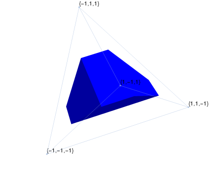
Figure 1: Possible Pauli channels when $S_{30}=0.5$ and $\gamma=0.6$, including the shrinking effect of Eq. (92). The hollow tetrahedron is $\mathcal{T}$ characterizing all Pauli channels, whilst the shaded region is the allowable values of $\mathbf{q}$ bounded by $(\;\;\;\frac{2}{\sqrt{7}},\pm\frac{1}{\sqrt{7}},\mp\frac{2}{7}),(\pm\frac{1}{\sqrt{7}},\;\;\;\frac{2}{\sqrt{7}},\mp\frac{2}{7}),(-\frac{2}{\sqrt{7}},\pm\frac{1}{\sqrt{7}},\pm\frac{2}{7}),\\ (\pm\frac{1}{\sqrt{7}},-\frac{2}{\sqrt{7}},\pm\frac{2}{7})$ for these particular values.

V Properties and capacities of Pauli-damping channels

Now that we have shown what channels can be simulated, we study some of the properties of these channels. First of all, we quantify how distinguishable they are from their closest Pauli equivalent. It turns out that the decomposition in Theorem 15 provides a simple answer to this problem: the distance is simply $\eta$.

V.1 Distance in trace norm

The trace norm distance between two quantum channels $\mathcal{E}_{1}$ and $\mathcal{E}_{2}$ can be defined as

$$||\mathcal{E}_{1}-\mathcal{E}_{2}||_{1}:=\sup_{\rho}||\mathcal{E}_{1}\left(\rho\right)-\mathcal{E}_{2}\left(\rho\right)||_{1}$$ (96)

where $||\sigma||_{1}=$Tr$\sqrt{\sigma\sigma^{\dagger}}$. For Hermitian matrices, this is equivalent to the sum of the absolute values of the eigenvalues of $\sigma$. We then state the following.

Proposition 18

Given a decomposition $\mathcal{E}_{\text{sim}}=\sigma_{x}^{u}\circ\mathcal{E}_{\eta}\circ\mathcal{E}_{P}$ characterized by $\eta$ and $(q_{1},q_{2},q_{3})$ respectively, then the trace norm between $\mathcal{E}_{\text{sim}}$ and the closest Pauli channel $\mathcal{E}_{\text{cl}}$ is simply $\eta$. Moreover, the closest Pauli channel has $(f_{11},f_{22},f_{33})=\begin{cases}\left(\sqrt{1-\eta}q_{1},-\sqrt{1-\eta}q_{2},\phantom{-}(1-\eta)q_{3}\right)&\mbox{ for }u=0,\\ \left(\sqrt{1-\eta}q_{1},\phantom{-}\sqrt{1-\eta}q_{2},-(1-\eta)q_{3}\right)&\mbox{ for }u=1.\end{cases}$

Proof. For qubits, the trace norm between two states is simply the Euclidean distance between their Bloch vectors. Therefore we have a very natural way to find the trace norm between two-qubit channels. When $u=0$, the Bloch vector of a state under $\mathcal{E}_{\text{sim}}$ is $\mathbf{r}_{\text{sim}}=(\sqrt{1-\eta}q_{1}x,-\sqrt{1-\eta}q_{2}y,(1-\eta)q_{3}z+\eta)$, whilst under an arbitrary Pauli channel it is $\mathbf{r}_{P}=(c_{1}x,-c_{2}y,c_{3}z)$. Thus the problem we need to solve is

$$\min_{\left(c_{1},c_{2},c_{3}\right)\in\mathcal{T}}\;\;\max_{x,y,z:x^{2}+y^{2}+z^{2}\leq 1}$$

$$\left((\sqrt{1-\eta}q_{1}-c_{1})x\right)^{2}+\left(-(\sqrt{1-\eta}q_{2}-c_{2})y\right)^{2}$$

$$+ \Big{(}((1-\eta)q_{3}-c_{3})z+\eta\Big{)}^{2},$$ (97)

which is the square of the trace norm. Let us first look at the final term $\left(\left((1-\eta)q_{3}-c_{3}\right)z+\eta\right)^{2}$. Given our maximum occurs for some fixed $|z|$ value, we have that the value of this term will be

$$\max\bigg{\{} \big{(}\left((1-\eta)q_{3}-c_{3}\right)|z|+\eta\big{)}^{2},$$

$$\big{(}-\left((1-\eta)q_{3}-c_{3}\right)|z|+\eta\big{)}^{2}\bigg{\}}$$

$$= \big{(}|(1-\eta)q_{3}-c_{3}||z|+\eta\big{)}^{2}.$$ (98)

Clearly this is minimized when $c_{3}=\left(1-\eta\right)q_{3}$, and has value $\eta^{2}$.

The remaining two parts of the equation are simpler. Clearly we want to set

$$c_{1}=\sqrt{1-\eta}q_{1},~{}c_{2}=\sqrt{1-\eta}q_{2},$$

to make these parts disappear, regardless of the values of $x$ and $y$. Thus we obtain our closest Pauli channel to be

$$(x,y,z)\rightarrow(\sqrt{1-\eta}q_{1}x,-\sqrt{1-\eta}q_{2}y,(1-\eta)q_{3}z).$$ (99)

We can be sure that this channel is Pauli as a consequence of Lemma 22 in Appendix C.
For the case when $u=1$, the proof is very similar, and given in Appendix C.$~{}\square$

V.2 Distance in diamond norm

It is not wise to use the trace norm as a measure for the distinguishability of channels, since it has been shown we can do it better in general by sending part of an entangled state through the channel Ent1 ; Ent2 ; Ent3 ; Ent4 ; Ent5 ; Ent6 . With this in mind, we look to an alternative distance. The diamond norm distance $||\mathcal{E}_{1}-\mathcal{E}_{2}||_{\diamond}$ is defined as:

$$||\mathcal{E}_{1}-\mathcal{E}_{2}||_{\diamond}:=\sup_{\rho\in\kappa\otimes\mathcal{H}}||\mathbb{I_{\kappa}}\otimes\mathcal{E}_{1}\left(\rho\right)-\mathbb{I_{\kappa}}\otimes\mathcal{E}_{2}\left(\rho\right)||_{1},$$ (100)

where $\mathrm{\kappa}$ in an ancillary Hilbert space to the one acted upon by $\mathcal{E}$, $\mathcal{H}$. In general, one has $||\mathcal{E}_{1}-\mathcal{E}_{2}||_{\diamond}\geq||\mathcal{E}_{1}-\mathcal{E}_{2}||_{1}$. Also we know that the diamond norm can be achieved with an ancillary Hilbert space $\kappa$ with $\text{dim}\;\kappa=\text{dim}\;\mathcal{H}~{}$Fano . Therefore, we need only consider a 1 qubit ancillary space in our case and state the following.

Proposition 19

For a channel $\mathcal{E}_{\text{sim}}=\sigma_{x}^{u}\circ\mathcal{E}_{\eta}\circ\mathcal{E}_{P}$, the closest Pauli channel under the diamond norm is the same as under the trace norm, given in Proposition 18, and the diamond norm distance is equal to $\eta$.

Sketch Proof. (Full proof in appendix C). First off, we know that

$$\min_{\mathcal{E}_{2}\in\text{Pauli}}||\mathcal{E}_{\text{sim}}-\mathcal{E}_{2}||_{\diamond}\leq||\mathcal{E}_{\text{sim}}-\mathcal{E}_{\text{cl}}||_{\diamond}.$$ (101)

In order to find the diamond norm between $\mathcal{E}_{\text{sim}}$ and $\mathcal{E}_{\text{cl}}$, we look at

$$||\mathbb{I}_{2}\otimes\mathcal{E}_{\text{sim}}\left(\rho\right)-\mathbb{I}_{2}\otimes\mathcal{E}_{\text{cl}}\left(\rho\right)||_{1}$$ (102)

for an arbitrary 2 qubit state $\rho$. We find the absolute sum of eigenvalues for $\mathbb{I}_{2}\otimes\mathcal{E}_{\text{sim}}\left(\rho\right)-\mathbb{I}_{2}\otimes\mathcal{E}_{\text{cl}}\left(\rho\right)$ to be independent of $\rho$ and equal to $\eta$. Thus we can conclude that

$$||\mathcal{E}_{\text{sim}}-\mathcal{E}_{\text{cl}}||_{\diamond}=\eta=||\mathcal{E}_{\text{sim}}-\mathcal{E}_{\text{cl}}||_{1}.$$ (103)

Using this, suppose there exists a channel $\mathcal{E}^{\prime}$ with a strictly smaller diamond norm than our closest channel. Then we have the chain of inequalities

$$||\mathcal{E}_{\text{sim}}-\mathcal{E}^{\prime}||_{1}\leq||\mathcal{E}_{\text{sim}}-\mathcal{E}^{\prime}||_{\diamond}<||\mathcal{E}_{\text{sim}}-\mathcal{E}_{\text{cl}}||_{\diamond}=||\mathcal{E}_{\text{sim}}-\mathcal{E}_{\text{cl}}||_{1}$$ (104)

leading to a contradiction, since we know the closest channel under trace norm to be $\mathcal{E}_{\text{cl}}$. Thus we are forced to conclude that the diamond norm is smallest between $\mathcal{E}_{\text{sim}}$ and $\mathcal{E}_{\text{cl}}$, with distance $\eta$. $\square$

The consequence of this result is that we have a natural measure of the generalization allowed by the introduction of classical channels. Given a resource state $\chi_{\gamma}$, we know that we will be able to simulate channels $||\cdot||_{\diamond}=\gamma$ distinct from the set of Pauli channels, since that is the largest allowable value $\eta$ may take.

V.3 Upper bound for the two-way private capacity

Now that we have characterized the class of Pauli-damping channels, we are interested in their quantum and private communication capacities. As explained in the introduction, the two-way assisted capacities are in general hard to calculate. Yet because we have shown that these channels can be simulated with an LOCC protocol (noisy teleportation) over a pre-shared resource (the amplitude damping Choi matrix $\chi_{\gamma}$), we may use teleportation stretching and Theorem 10 to upper-bound their two-way quantum ($Q_{2}$) and private capacities ($P_{2}=K$). In fact, for an arbitrary Pauli-damping channel $\mathcal{E}$ with resource state $\chi_{\gamma}$, we may compute the upper bound (weak converse)

$$Q_{2}(\mathcal{E})\leq P_{2}(\mathcal{E})=K(\mathcal{E})\leq E_{R}\left(\chi_{\gamma}\right)$$

$$\leq\frac{1}{2}-\frac{1-\gamma}{2}\log_{2}\left(\frac{1-\gamma}{2}\right)+\frac{2-\gamma}{2}\log_{2}\left(\frac{2-\gamma}{2}\right).$$ (105)

Within the Pauli-damping class, let us analyze the “squared” channel $\mathcal{E}_{\text{sq}}$ with its F matrix being given by

$$F_{\text{sq}}=\left(\begin{array}[c]{cccc}1&0&0&0\\ 0&\sqrt{1-\gamma}\left(1-\frac{\gamma}{2}\right)&0&0\\ 0&0&\sqrt{1-\gamma}\left(1-\frac{\gamma}{2}\right)&0\\ \gamma^{2}&0&0&(1-\gamma)^{2}\end{array}\right).$$ (106)

The decomposition of this channel into the form (61) of Theorem 15 is $u=0$, $\eta=\gamma^{2}$, and

$$\mathbf{q}=\left(\frac{\left(1-\frac{\gamma}{2}\right)}{\sqrt{1+\gamma}},-\frac{\left(1-\frac{\gamma}{2}\right)}{\sqrt{1+\gamma}},\frac{1-\gamma}{1+\gamma}\right),$$ (107)

where $\gamma$ is the damping parameter of the resource state. Its two-way quantum and private capacities are upper bounded by using Eq. (105) and lower bounded by optimizing the coherent information of the channel. The results are shown in Fig. 2.

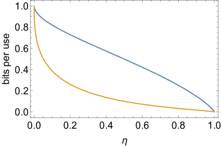
Figure 2: Upper and lower bounds for the two-way private capacity $P_{2}$ and the two-way quantum capacity $Q_{2}$ of the squared channel $\mathcal{E}_{\text{sq}}$, in terms of its parameter $\eta$ which is the square of the amplitude damping parameter $\gamma$ associated with its resource state.

VI Conclusions

In this paper we have studied a particular design for the LOCC simulation of quantum channels. This design is based on a modified teleportation protocol where not only the resource state is generally mixed (instead of maximally entangled) but also the classical communication channel between the parties is noisy, i.e., affected by a classical channel. The latter feature allows us to simulate family of quantum channels, much larger than the Pauli class, for which we have provided a characterization in Theorem 11.

Starting from the Choi matrix of an amplitude damping channel as a resource state for the noisy teleportation protocol, we can easily simulate non-Pauli channels. In particular, we have introduced a new class of simulable channels, that we have called Pauli-damping channels. Their distance from the set of Pauli channels can be quantified in terms of the diamond norm and turns out to be easily related with the damping probability associated with the generating Choi matrix. For these Pauli-damping channels we have then used the method of teleportation stretching to derive upper bounds for their two-way quantum and private capacities.

In conclusion, our results are useful to shed new light in the area of channel simulation with direct implications for quantum and private communication with qubit systems. Further developments may include the study of Pauli-damping channels in the context of adaptive quantum metrology Metro , or in the setting of secure quantum networks networkPIRS .

Acknowledgments. This work has been supported by the EPSRC via the ‘UK Quantum Communications Hub’ (EP/M013472/1). T.C. and S.P. would like to thank discussions with R. Laurenza and C. Ottaviani. L.H. would like to thank the ERASMUS program who allowed him to visit the University of York, where this work has been carried out. T.C. acknowledges funding from a White Rose Scholarship. L.B. has received funding for this research from the European Research Council under the European Union Seventh Framework Programme (FP7/2007-2013)/ERC Grant Agreement No. 308253 PACOMANEDIA.

Appendix A Proof of Theorem 8

Let us suppose that the channel $\mathcal{E}(\rho_{C})$ is Choi-stretchable via a WH-teleportation protocol. This means that

$$\mathcal{E}(\rho_{C}) =\Gamma_{\chi_{\mathcal{E}}}(\rho_{C})=\sum_{g\in G}V_{B}^{\dagger}(g)\mathrm{Tr}_{CA}\left(E_{CA}(g)(\rho_{C}\otimes\chi_{\mathcal{E}})\right)V_{B}(g).$$ (108)

Now consider $V_{B}^{\dagger}(h)\mathcal{E}\left(U_{C}(h)\rho_{C}U_{C}^{\dagger}(h)\right)V_{B}(h)$ which expands out to

$$V_{B}^{\dagger}(h)\left(\sum_{g\in G}V_{B}^{\dagger}(g)\mathrm{Tr}_{CA}\left(E_{CA}(g)(U_{C}(h)\rho_{C}U_{C}^{\dagger}(h)\otimes\chi_{\mathcal{E}})\right)V_{B}(g)\right)V_{B}(h)$$ (109)

$$= \sum_{g\in G}V_{B}^{\dagger}(h)V_{B}^{\dagger}(g)\mathrm{Tr}_{CA}\left(E_{CA}(g)(U_{C}(h)\rho_{C}U_{C}^{\dagger}(h)\otimes\chi_{\mathcal{E}})\right)V_{B}(g)V_{B}(h).$$ (110)

Since $\left\{V_{B}(g)\right\}$ is a representation of the WH-group, we may use $V_{B}(g)V_{B}(h)=e^{i\phi(g,h)}V_{B}(gh)$,
where $e^{i\phi(g,h)}$ is some overall phase.

$$\mathrm{Eq.~{}(\ref{A4})}= \sum_{g\in G}V_{B}^{\dagger}(gh)\mathrm{Tr}_{CA}\left(U_{C}^{\dagger}(h)E_{CA}(g)U_{C}(h)(\rho_{C}\otimes\chi_{\mathcal{E}})\right)V_{B}(gh)$$ (111)

$$= \sum_{g\in G}V_{B}^{\dagger}(gh)\mathrm{Tr}_{CA}\left(U_{C}^{\dagger}(h)U_{C}^{\dagger}(g)\ket{\Phi}\bra{\Phi}U_{C}(g)U_{C}(h)(\rho_{C}\otimes\chi_{\mathcal{E}})\right)V_{B}(gh)$$ (112)

$$= \sum_{g\in G}V_{B}^{\dagger}(gh)\mathrm{Tr}_{CA}\left(U_{C}^{\dagger}(gh)\ket{\Phi}\bra{\Phi}U_{C}(gh)(\rho_{C}\otimes\chi_{\mathcal{E}})\right)V_{B}(gh)$$ (113)

$$= \sum_{g\in G}V_{B}^{\dagger}(gh)\mathrm{Tr}_{CA}\left(E_{CA}(gh)(\rho_{C}\otimes\chi_{\mathcal{E}})\right)V_{B}(gh).$$ (114)

Now we may use the group property that $gG=G$, for any $g\in G$

$$\mathrm{Eq.~{}(\ref{A8})}= \sum_{g^{\prime}\in G}V_{B}^{\dagger}(g^{\prime})\mathrm{Tr}_{CA}\left(E_{CA}(g^{\prime})(\rho_{C}\otimes\chi_{\mathcal{E}})\right)V_{B}(g^{\prime})\phantom{\mathrm{Tr}_{CA}\left(E_{CA}(g^{\prime})(\rho_{C}\otimes\chi_{\mathcal{E}})\right)}$$ (115)

$$= \Gamma_{\chi_{\mathcal{E}}}(\rho_{C})=\mathcal{E}(\rho_{C}).$$ (116)

We can therefore conclude that Choi-stretchable channels via WH-teleportation are teleportation covariant. $\square$

We could also consider a more general case, where we have a channel in the form seen in Eq. (37), but without the group representation structure. However, we would not expect this to be covariant, since Eq. (35) forces

$$V(gh)\mathcal{E}(\rho)V^{\dagger}(gh) =\mathcal{E}(U(gh)\rho U^{\dagger}(gh))$$

$$=\mathcal{E}(U(g)U(h)\rho U^{\dagger}(h)U^{\dagger}(g))$$

$$=V(g)\mathcal{E}(U(h)\rho U^{\dagger}(h))V^{\dagger}(g)$$

$$=V(g)V(h)\mathcal{E}(\rho)V^{\dagger}(h)V^{\dagger}(g).$$

Appendix B The form of $S_{ij}$

In this section, we present the 12 possible forms for $S_{ij}$ in a concise way. We present a $3\times 4$ matrix, $\bm{\mathcal{S}}$ of $4\times 4$ matrices. The rows of $\bm{\mathcal{S}}$ correspond to $i=1,2,3$ respectively, and the columns to $j=0,1,2,3$. Given $i,j$^th element $\bm{\mathcal{S}}_{ij}$, $S_{ij}$ can be obtained by the sum $\sum_{k=0,l=0}^{3,3}(\bm{\mathcal{S}}_{ij})_{k,l}\;p_{l|k}$ - note we are counting the rows and columns of $\bm{\mathcal{S}}_{ij}$ from $0$.

$$\bm{\mathcal{S}}=\left(\begin{array}[]{cccc}\left(\begin{array}[]{cccc}1&1&-1&-1\\ 1&1&-1&-1\\ 1&1&-1&-1\\ 1&1&-1&-1\\ \end{array}\right)&\left(\begin{array}[]{cccc}1&1&-1&-1\\ 1&1&-1&-1\\ -1&-1&1&1\\ -1&-1&1&1\\ \end{array}\right)&\left(\begin{array}[]{cccc}-1&-1&1&1\\ 1&1&-1&-1\\ -1&-1&1&1\\ 1&1&-1&-1\\ \end{array}\right)&\left(\begin{array}[]{cccc}1&1&-1&-1\\ -1&-1&1&1\\ -1&-1&1&1\\ 1&1&-1&-1\\ \end{array}\right)\\[28.45274pt] \left(\begin{array}[]{cccc}1&-1&1&-1\\ 1&-1&1&-1\\ 1&-1&1&-1\\ 1&-1&1&-1\\ \end{array}\right)&\left(\begin{array}[]{cccc}1&-1&1&-1\\ 1&-1&1&-1\\ -1&1&-1&1\\ -1&1&-1&1\\ \end{array}\right)&\left(\begin{array}[]{cccc}-1&1&-1&1\\ 1&-1&1&-1\\ -1&1&-1&1\\ 1&-1&1&-1\\ \end{array}\right)&\left(\begin{array}[]{cccc}1&-1&1&-1\\ -1&1&-1&1\\ -1&1&-1&1\\ 1&-1&1&-1\\ \end{array}\right)\\[28.45274pt] \left(\begin{array}[]{cccc}1&-1&-1&1\\ 1&-1&-1&1\\ 1&-1&-1&1\\ 1&-1&-1&1\\ \end{array}\right)&\left(\begin{array}[]{cccc}1&-1&-1&1\\ 1&-1&-1&1\\ -1&1&1&-1\\ -1&1&1&-1\\ \end{array}\right)&\left(\begin{array}[]{cccc}-1&1&1&-1\\ 1&-1&-1&1\\ -1&1&1&-1\\ 1&-1&-1&1\\ \end{array}\right)&\left(\begin{array}[]{cccc}1&-1&-1&1\\ -1&1&1&-1\\ -1&1&1&-1\\ 1&-1&-1&1\\ \end{array}\right)\\[28.45274pt] \end{array}\right)$$

Appendix C Proofs

Lemma 20

$\frac{1-\gamma}{1-\gamma S_{30}}\in[0,1]$

Proof. Remember that $\gamma\in[0,1]$. Therefore $1-\gamma\in[0,1]$ also.
Now, $S_{30}\in[0,1]$ in the first case. Thus,

$$\gamma S_{30} \leq\gamma$$

$$\Rightarrow-\gamma S_{30} \geq-\gamma$$

$$\Rightarrow 1-\gamma S_{30} \geq 1-\gamma$$

$$\Rightarrow 1 \geq\frac{1-\gamma}{1-\gamma S_{30}}$$

remembering $1-\gamma S_{30}\geq 0$. $\square$

Corollary 21

$\sqrt{\frac{1-\gamma}{1-\gamma S_{30}}}\in[0,1]$.

Lemma 22

If a point $(x,y,z)$ belongs to the tetrahedron defined by $\mathcal{T}$, then so too does the point $(\sqrt{\alpha}x,\sqrt{\alpha}y,\alpha z)$,where $\alpha\in[0,1]$

Proof. Since any point in the tetrahedron can be expressed as a convex combination of the four extremal points in $\mathcal{T}$, it is sufficient to show that the four points,

$$(\phantom{-}\sqrt{\alpha},-\sqrt{\alpha},\phantom{-}\alpha), (\phantom{-}\sqrt{\alpha},\phantom{-}\sqrt{\alpha},-\alpha),$$ (117)

$$(-\sqrt{\alpha},\phantom{-}\sqrt{\alpha},\phantom{-}\alpha), (-\sqrt{\alpha},-\sqrt{\alpha},-\alpha),$$

belong to the tetrahedron (i.e. are themselves a convex combination of the four extremal points), and thus any rescaled tetrahedron point also still remains with the full tetrahedron.
Expressing any point as

$$(x,y,z) =p_{0}(\phantom{-}1,-1,\phantom{-}1)+p_{1}(\phantom{-}1,\phantom{-}1,-1)$$

$$+p_{2}(-1,-1,-1)+p_{3}(-1,\phantom{-}1,\phantom{-}1),$$

$$p_{0}+p_{1}+p_{2}+p_{3}=1,\;\;p_{i}\geq 0$$

then we can achieve the points in Eq. (117)

$$\begin{array}[]{ccccc}\text{Point}&p_{0}&p_{1}&p_{2}&p_{3}\\ (\sqrt{\alpha},-\sqrt{\alpha},\alpha)&\frac{(1+\sqrt{\alpha})^{2}}{4}&\frac{1-\alpha}{4}&\frac{1-\alpha}{4}&\frac{(1-\sqrt{\alpha})^{2}}{4}\\ (\sqrt{\alpha},\sqrt{\alpha},-\alpha)&\frac{1-\alpha}{4}&\frac{(1-\sqrt{\alpha})^{2}}{4}&\frac{(1+\sqrt{\alpha})^{2}}{4}&\frac{1-\alpha}{4}\\ (-\sqrt{\alpha},\sqrt{\alpha},\alpha)&\frac{(1-\sqrt{\alpha})^{2}}{4}&\frac{1-\alpha}{4}&\frac{1-\alpha}{4}&\frac{(1+\sqrt{\alpha})^{2}}{4}\\ (-\sqrt{\alpha},-\sqrt{\alpha},-\alpha)&\frac{1-\alpha}{4}&\frac{(1+\sqrt{\alpha})^{2}}{4}&\frac{(1-\sqrt{\alpha})^{2}}{4}&\frac{1-\alpha}{4}.\\ \end{array}$$ (118)

The normalization and positivity conditions are easy to verify. $\square$

Corollary 23

If $\left(S_{11},S_{22},S_{33}\right)$ belongs to tetrahedron $\mathcal{T}$, then so too does

$$\left(\sqrt{\frac{1-\gamma}{1-\gamma S_{30}}}S_{11},\sqrt{\frac{1-\gamma}{1-\gamma S_{30}}}S_{22},\frac{1-\gamma}{1-\gamma S_{30}}S_{33}\right)$$ (119)

$$=\;\; (q_{1},q_{2},q_{3})$$

Proof. We can simply set $\alpha=\frac{1-\gamma}{1-\gamma S_{30}}$, and apply Lemma 22. $\square$

Lemma 24

For all classical channels $\Pi$, as defined in our noisy teleportation protocol, we have that $(S_{11},S_{22},S_{33})$ belongs to the tetrahedron $\mathcal{T}$.

Proof. An alternative way to define $\mathcal{T}$ is by four inequalities which are satisfied by all points within the tetrahedron, namely

$$x+y+z \leq 1$$

$$x-y-z \leq 1$$

$$-x+y-z \leq 1$$

$$-x-y+z \leq 1$$

We have already seen these used in Section II.2. Testing these with $S_{11},S_{22}$ and $S_{33}$ we find

$$S_{11}+S_{22}+S_{33} =1-(p_{02}+p_{13}+p_{20}+p_{31})\leq 1$$

$$S_{11}-S_{22}-S_{33} =1-(p_{03}+p_{12}+p_{21}+p_{30})\leq 1$$

$$-S_{11}+S_{22}-S_{33} =1-(p_{00}+p_{11}+p_{22}+p_{33})\leq 1$$

$$-S_{11}-S_{22}+S_{33} =1-(p_{01}+p_{10}+p_{23}+p_{32})\leq 1.$$

From this, we can conclude that all $(S_{11},S_{22},S_{33})$ possible belong to the tetrahedron. This immediately gives that, in the case where $S_{30}\geq 0$ our decomposition is a valid one. $\square$

Proof of Theorem 15 for $S_{30}\leq 0$.
We have already proven this result to be true for $S_{30}\geq 0$ in the main body of the text. We also need to consider our second case, $S_{30}\leq 0$. Here we set $\eta=-\gamma S_{30}$. This time we obtain

$$(q_{1},q_{2},q_{3})=\bigg{(}\frac{\sqrt{1-\gamma}}{\sqrt{1+\gamma S_{30}}} S_{11},$$

$$-\frac{\sqrt{1-\gamma}}{\sqrt{1+\gamma S_{30}}} S_{22},$$

$$-\frac{1-\gamma}{1+\gamma S_{30}} S_{33}\bigg{)}$$ (120)

Except for the fact our scaling factor is now $\frac{1-\gamma}{1+\gamma S_{30}}$, we have a very similar situation to our first case, except now we need to prove that $(S_{11},-S_{22},-S_{33})$ is in the tetrahedron, in order for our decomposition to be valid for our second scenario. If we look at the four inequalities that we need to satisfy, we find that

$$S_{11}+(-S_{22})+(-S_{33}) =S_{11}-S_{22}-S_{33}$$

$$S_{11}-(-S_{22})-(-S_{33}) =S_{11}+S_{22}+S_{33}$$

$$-S_{11}+(-S_{22})-(-S_{33}) =-S_{11}-S_{22}+S_{33}$$

$$-S_{11}-(-S_{22})+(-S_{33}) =-S_{11}+S_{22}-S_{33}.$$

which we already know satisfy our tetrahedron inequalities. Thus we have proved that our decomposition is valid too for cases where $S_{30}\leq 0$, and so is true for all channels simulable with $\chi_{\gamma}$ as a resource.$\square$

Proof of Proposition 18 with $u=1$.
In this case, we have to contend with the sign change enacted by $\sigma_{x}$; however the proof is similar. This time, we aim to solve

$$\min_{\left(c_{1},c_{2},c_{3}\right)\in\mathcal{T}}\;\;\max_{x,y,z:x^{2}+y^{2}+z^{2}\leq 1}$$

$$\left((\sqrt{1-\eta}q_{1}-c_{1})x\right)^{2}+\left((\sqrt{1-\eta}q_{2}+c_{2})y\right)^{2}$$

$$+ \Big{(}(-(1-\eta)q_{3}-c_{3})z-\eta\Big{)}^{2}.$$ (121)

Again, we begin by looking at the final part of the sum. For a fixed value of $|z|$, this term will be

$$\max\bigg{\{} \big{(}\left(-(1-\eta)q_{3}-c_{3}\right)|z|-\eta\big{)}^{2},$$

$$\big{(}\left((1-\eta)q_{3}+c_{3}\right)|z|-\eta\big{)}^{2}\bigg{\}}$$

$$=\max\bigg{\{} \big{(}\left((1-\eta)q_{3}+c_{3}\right)|z|+\eta\big{)}^{2},$$

$$\big{(}-\left((1-\eta)q_{3}+c_{3}\right)|z|+\eta\big{)}^{2}\bigg{\}}$$

$$= \big{(}|(1-\eta)q_{3}+c_{3}||z|+\eta\big{)}^{2}.$$ (122)

This is clearly minimized when $c_{3}=-(1-\eta)q_{3}$. For the $x$ and $y$ terms, they are clearly minimized for

$$c_{1}=\sqrt{1-\eta}q_{1},~{}c_{2}=-\sqrt{1-\eta}q_{2}.$$

Remembering that $\mathcal{T}$ is invariant under $\sigma_{x}$, and thus if $(q_{1},q_{2},q_{3})$ belongs to the tetrahedron so too does $(q_{1},-q_{2},-q_{3})$, therefore we can again conclude that the channel corresponding to $(c_{1},c_{2},c_{3})$ is Pauli, and our second part of the proposition is proved. $\square$

Lemma 25

$||\mathcal{E}_{1}-\mathcal{E}_{2}||_{\diamond}\geq||\mathcal{E}_{1}-\mathcal{E}_{2}||_{1}$.

Proof.

$$||\mathcal{E}_{1}-\mathcal{E}_{2}||_{\diamond} =\sup_{\rho\in\kappa\otimes\mathcal{H}}||\mathrm{I_{\kappa}}\otimes\mathcal{E}_{1}\left(\rho\right)-\mathrm{I_{\kappa}}\otimes\mathcal{E}_{2}\left(\rho\right)||_{1}$$ (123)

$$\geq\sup_{\rho\in\text{sep}\left(\kappa\otimes\mathcal{H}\right)}||\mathrm{I_{\kappa}}\otimes\mathcal{E}_{1}\left(\rho\right)-\mathrm{I_{\kappa}}\otimes\mathcal{E}_{2}\left(\rho\right)||_{1}$$ (124)

$$=\sup_{\rho_{1}\otimes\rho_{2}}||\mathrm{I_{\kappa}}\otimes\mathcal{E}_{1}\left(\rho_{1}\otimes\rho_{2}\right)-\mathrm{I_{\kappa}}\otimes\mathcal{E}_{2}\left(\rho_{1}\otimes\rho_{2}\right)||_{1}$$ (125)

$$=\sup_{\rho_{1}\otimes\rho_{2}}||\rho_{1}\otimes\mathcal{E}_{1}\left(\rho_{2}\right)-\rho_{1}\otimes\mathcal{E}_{2}\left(\rho_{2}\right)||_{1}$$ (126)

$$=\sup_{\rho_{2}}||\mathcal{E}_{1}\left(\rho_{2}\right)-\mathcal{E}_{2}\left(\rho_{2}\right)||_{1}$$ (127)

$$=||\mathcal{E}_{1}-\mathcal{E}_{2}||_{1}.$$ (128)

Note we have used the property of subadditivity over tensor product of the trace norm. $\square$

Full proof of Proposition 19.
We shall begin with the case where $u=0$. First off, we know that

$$\min_{\mathcal{E}_{2}\in\text{Pauli}}||\mathcal{E}_{\text{sim}}-\mathcal{E}_{2}||_{\diamond}\leq||\mathcal{E}_{\text{sim}}-\mathcal{E}_{\text{cl}}||_{\diamond}.$$ (129)

In order to find the diamond norm between $\mathcal{E}_{\text{sim}}$ and $\mathcal{E}_{\text{cl}}$, we look at

$$||\mathbb{I}_{2}\otimes\mathcal{E}_{\text{sim}}\left(\rho\right)-\mathbb{I}_{2}\otimes\mathcal{E}_{\text{cl}}\left(\rho\right)||_{1}$$ (130)

for an arbitrary 2 qubit state $\rho$. We find the matrix $M_{D}=\left(\mathbb{I}_{2}\otimes\mathcal{E}_{\text{sim}}\left(\rho\right)-\mathbb{I}_{2}\otimes\mathcal{E}_{\text{cl}}\left(\rho\right)\right)$ to be

$$M_{D}=\frac{1}{4}\left(\begin{array}[]{cccc}(1+a_{3})\eta&0&(a_{1}-\mathrm{i}a_{2})\eta&0\\ 0&1(1+a_{3})\eta&0&-(a_{1}-\mathrm{i}a_{2})\eta\\ (a_{1}+\mathrm{i}a_{2})\eta&0&(1-a_{3})\eta&0\\ 0&-(a_{1}+\mathrm{i}a_{2})\eta&0&(-1+a_{3})\eta\end{array}\right)$$ (131)

which has eigenvalues

$$\frac{1}{4}\Big{(}-1- \sqrt{a_{1}^{2}+a_{2}^{2}+a_{3}^{2}}\Big{)}\eta \frac{1}{4}\Big{(}1- \sqrt{a_{1}^{2}+a_{2}^{2}+a_{3}^{2}}\Big{)}\eta$$ (132)

$$\frac{1}{4}\Big{(}-1+ \sqrt{a_{1}^{2}+a_{2}^{2}+a_{3}^{2}}\Big{)}\eta \frac{1}{4}\Big{(}1+ \sqrt{a_{1}^{2}+a_{2}^{2}+a_{3}^{2}}\Big{)}\eta.$$

Remembering that $$a_{1}^{2}+a_{2}^{2}+a_{3}^{2}\leq 1$$, this means the singular values are:

$$\frac{1}{4}\Big{(}1+ \sqrt{a_{1}^{2}+a_{2}^{2}+a_{3}^{2}}\Big{)}\eta \frac{1}{4}\Big{(}1- \sqrt{a_{1}^{2}+a_{2}^{2}+a_{3}^{2}}\Big{)}\eta$$ (133)

$$\frac{1}{4}\Big{(}1- \sqrt{a_{1}^{2}+a_{2}^{2}+a_{3}^{2}}\Big{)}\eta \frac{1}{4}\Big{(}1+ \sqrt{a_{1}^{2}+a_{2}^{2}+a_{3}^{2}}\Big{)}\eta,$$

and thus their sum is $\eta$. This gives $||\mathcal{E}_{\text{sim}}-\mathcal{E}_{\text{cl}}||_{\diamond}=\eta=||\mathcal{E}_{\text{sim}}-\mathcal{E}_{\text{cl}}||_{1}$.
Using this, suppose there exists a channel $\mathcal{E}^{\prime}$ with a strictly smaller diamond norm than our closest channel. Then we have the chain of inequalities

$$||\mathcal{E}_{\text{sim}}-\mathcal{E}^{\prime}||_{1}\leq||\mathcal{E}_{\text{sim}}-\mathcal{E}^{\prime}||_{\diamond}<||\mathcal{E}_{\text{sim}}-\mathcal{E}_{\text{cl}}||_{\diamond}=\eta=||\mathcal{E}_{\text{sim}}-\mathcal{E}_{\text{cl}}||_{1},$$ (134)

leading to a contradiction, since we know the closest channel under trace norm to be $\mathcal{E}_{\text{cl}}$. Thus we are forced to conclude that the diamond norm is smallest between $\mathcal{E}_{\text{sim}}$ and $\mathcal{E}_{\text{cl}}$, with distance $\eta$.

In the case where $u=1$, we are writing $\mathcal{E}_{\text{sim}}$ as the unitary $\sigma_{x}$ applied after a similar simulable channel, $\mathcal{E}_{\text{pos}}=\mathcal{E}_{\eta}\circ\mathcal{E}_{P}$. This has closest Pauli channel $\mathcal{E}_{\text{poscl}}=\left(\sqrt{1-\eta}q_{1},\sqrt{1-\eta}q_{2},(1-\eta)q_{3}\right)$. Since the trace norm is invariant under unitaries, and the 2 qubit channel $\mathbb{I}_{2}\otimes\sigma_{x}$ is unitary, we can conclude that

$$\phantom{=}||\mathcal{E}_{\text{pos}}-\mathcal{E}_{\text{poscl}}||_{\diamond}$$

$$=\sup_{\rho}||\mathbb{I}_{2}\otimes\mathcal{E}_{\text{pos}}\left(\rho\right)-\mathbb{I}_{2}\otimes\mathcal{E}_{\text{poscl}}\left(\rho\right)||_{1}$$

$$=\sup_{\rho}||\left(\mathbb{I}_{2}\otimes\sigma_{x}\right)\left(\mathbb{I}_{2}\otimes\mathcal{E}_{\text{pos}}\left(\rho\right)-\mathbb{I}_{2}\otimes\mathcal{E}_{\text{poscl}}\left(\rho\right)\right)||_{1}$$

$$=\sup_{\rho}||\mathbb{I}_{2}\otimes\mathcal{E}_{\text{sim}}\left(\rho\right)-\mathbb{I}_{2}\otimes\mathcal{E}_{\text{cl}}\left(\rho\right)||_{1}$$

$$=||\mathcal{E}_{\text{sim}}-\mathcal{E}_{\text{cl}}||_{\diamond},$$

where we have spotted that the channel $\mathcal{E}_{\text{cl}}=\sigma_{x}\otimes\mathcal{E}_{\text{poscl}}$. We can then conclude that $||\mathcal{E}_{\text{sim}}-\mathcal{E}_{\text{cl}}||_{\diamond}=\eta$, and therefore by using the same chain of inequalities (104), we force this to be the minimum distance possible. $\square$

References

- (1) M. A. Nielsen, and I. L. Chuang, Quantum computation and quantum information (Cambridge University Press, Cambridge, 2000).
- (2) J. Preskill, Lecture Notes for Physics 229: Quantum Information and Computation, available at http://www.theory.caltech.edu/people/preskill/ph229/ (Accessed 18 May 2017).
- (3) C. Weedbrook et al., Rev. Mod. Phys. 84, 621 (2012).
- (4) S. L. Braunstein, and P. Van Loock, Rev. Mod. Phys. 77, 513 (2005).
- (5) C. H. Bennett, D. P. DiVincenzo, J. A. Smolin, and W. K. Wootters, Phys. Rev. A 54, 3824-3851 (1996).
- (6) C. H. Bennett, G. Brassard, C. Crepeau, R. Jozsa, A. Peres, and W. K. Wootters, Phys. Rev. Lett. 70, 1895 (1993).
- (7) S. Pirandola, J. Eisert, C. Weedbrook, A. Furusawa, and S. L. Braunstein, Advances in quantum teleportation, Nature Photon. 9, 641-652 (2015).
- (8) Garry Bowen and Sougato Bose, Phys. Rev. Lett. 87, 26 (2001).
- (9) M. Horodecki, P. Horodecki, and R. Horodecki, Phys. Rev. A 99, 1888–1898 (1999).
- (10) R. F. Werner, J. Phys. A 34, 7081–7094 (2001).
- (11) D. Leung, and W. Matthews, IEEE Transactions on Information Theory, 61, 4486–4499 (2015).
- (12) S. Pirandola, R. Laurenza, C. Ottaviani and L. Banchi, Nature Communications 8, 15043 (2017). See also arXiv:1510.08863 (2015).
- (13) M .M. Wilde, M. Tomamichel, and M. Berta, arXiv.org/abs/1602.08898 (2016).
- (14) Advances on channel simulation are explained in detail in the Supplementary Note 8 of Ref. Stretching .
- (15) A. Müller-Hermes, Transposition in Quantum Information Theory, (Master Thesis, Technische Universität München, 2012).
- (16) J. Niset, J. Fiurasek, and N. J. Cerf, Phys. Rev. Lett. 102, 120501 (2009).
- (17) M. M. Wolf, Notes on “Quantum Channels & Operations” (see page 36). Available at https://www-m5.ma.tum.de/foswiki/pub/M5/Allgemeines/ MichaelWolf/QChannelLecture.pdf.
- (18) S. Pirandola, S. Capacities of repeater-assisted quantum communications, Preprint arXiv:1601.00966 (2016).
- (19) R. Laurenza, and S. Pirandola, General bounds for sender-receiver capacities in multipoint quantum communications, Preprint arxiv:1603.07262 (2016).
- (20) S. Pirandola, and C. Lupo, Phys. Rev. Lett. 118, 100502 (2017).
- (21) Advances in the reduction of adaptive protocols are explained in detail in Supplementary Note 9 of Ref. Stretching .
- (22) V. Vedral, Rev. Mod. Phys. 74, 197 (2002).
- (23) V. Vedral, M. B. Plenio, M. A. Rippin, and P. L. Knight, Phys. Rev. Lett. 78, 2275-2279 (1997).
- (24) V. Vedral, and M. B. Plenio, Phys. Rev. A 57, 1619 (1998).
- (25) C. H. Bennett, D. P. DiVincenzo, and J. A. Smolin, Phys. Rev. Lett. 78, 3217–3220 (1997).
- (26) K. Goodenough, D. Elkouss, and S. Wehner, New J. Phys. 18, 063005 (2016); Preprint arXiv:1511.08710v1 (2015).
- (27) R. García-Patrón, S. Pirandola, S. Lloyd, and J. H. Shapiro, Phys. Rev. Lett. 102, 210501 (2009).
- (28) S. Pirandola, R. García-Patrón, S. L. Braunstein, and S. Lloyd, Phys. Rev. Lett. 102, 050503 (2009).
- (29) R. Namiki, L. Jiang, J. Kim, and N. Lütkenhaus, Phys. Rev. A 94, 052304 (2016).
- (30) M. Pant, H. Krovi, D. Englund, and S. Guha, Phys. Rev. A 95, 012304 (2017).
- (31) F. Ewert and P. van Loock, Phys. Rev. A 95, 012327 (2017).
- (32) A. Khalique and B. C. Sanders, Opt. Eng. 56, 016114 (2017).
- (33) F. Rozpedek et al., Preprint arXiv:1705.00043 (2017)
- (34) As a clarification on the literature, let us remark that the contribution of Ref. WildeFollowup is about this strong converse refinement. There is no “solidification” of the weak converse bounds and two-way capacities previously established by Ref. Stretching , already fully computed in the first 2015 arXiv papers first ; secondP . In these papers, the treatment of the shield system (which intervenes in definition of private state KD ) is completely correct by an immediate application of a previous argument Matthias1a ; Matthias2a which showed the exponential increase of the shield size for DV systems. This argument can be found in Eq. (21) of Ref. (first, , Version 2) for the case of DV channels. The extension to CV channels is achieved by just truncating the Hilbert space, as explicitly discussed afer Eq. (23) of Ref. (first, , Version 2). The correctness of this approach has been also confirmed by later equivalent proofs present in the published version of the manuscript Stretching , one of which does not even depend on the shield system. See Supplementary Note 3 of Ref. Stretching for full details.
- (35) S. Pirandola, R. Laurenza, C. Ottaviani and L. Banchi, Preprint arXiv:1510.08863 (Version 1, 29 October 2015; Version 2, 8 December 2015).
- (36) S. Pirandola, and R. Laurenza, General Benchmarks for Quantum Repeaters, Preprint arxiv:1512.04945 (15 December 2015).
- (37) K. Horodecki, M. Horodecki, P. Horodecki, and J. Oppenheim, Phys. Rev. Lett. 94, 160502 (2005).
- (38) M. Christandl, A. Ekert, M. Horodecki, P. Horodecki, J. Oppenheim, and R. Renner, Lecture Notes in Computer Science 4392, 456-478 (2007). See also arXiv:quant-ph/0608199v3 for a more extended version.
- (39) M. Christandl, N. Schuch, and A. Winter, Comm. Math. Phys. 311, 397-422 (2012).
- (40) L. Vaidman, Phys. Rev. A 49, 1473–1476 (1994).
- (41) S. L. Braunstein and H. J. Kimble, Phys. Rev. Lett. 80, 4084 (1998).
- (42) S. L. Braunstein, G. M. D’Ariano, G. J. Milburn, and M. F. Sacchi, Phys. Rev. Lett. 84, 3486–3489 (2000).
- (43) S. Pirandola, and S. Mancini, Laser Physics 16, 1418 (2006).
- (44) R. Horodecki and M. Horodecki, Phys, Rev. A 54:3, 1838-1843 (1996).
- (45) Note that, in a quantum communication scenario, the most general type of channel simulation must be based on LOCCs, because Alice and Bob are remote parties and may only apply operations on their local systems. Furthermore, the simplification of the capacity upper bound, based the relative entropy of entanglement, exploits the requirement for trace-preserving LOCCs. However, in other scenarios (e.g., quantum computing or quantum metrology), we do not require remote parties and we may think of Alice and Bob to be the same entity. In this context, one can allow for types of channel simulation which are based on joint quantum operations, i.e., non-local between Alice and Bob qsim0 ; qsim1 ; qsim2 ; qsim3 . It is also clear that in general one may simulate a quantum channel by performing a dilation into an environment which is prepared into a pure or a mixed state Arvind .
- (46) M. A. Nielsen, and I. J. Chuang, Phys. Rev. Lett. 79, 321–324 (1997).
- (47) S. Ishizaka, and T. Hiroshima, Phys. Rev. Lett. 101, 240501 (2008).
- (48) Z. Ji, G. Wang, R. Duan, Y. Feng, and M. Ying, IEEE Trans. Inform. Theory 54, 5172–5185 (2008).
- (49) J. Kolodynski and R. Demkowicz-Dobrzanski, New J. Phys. 15, 073043 (2013).
- (50) G. Narang and Arvind, Phys. Rev. A 75, 032305 (2007).
- (51) C. Shannon, A Mathematical Theory of Communication Bell System Technical Journal 27:3, 379-423 (1948).
- (52) S. Lörwald and G. Reinelt, PANDA: A Software for Polyhedral Transformations, EURO Journal on Computational Optimization 3, 297-308 (2015).
- (53) A. Acín, Phys. Rev. Lett. 87, 177901 (2001).
- (54) G. M. D’Ariano, P. Lo Presti and M. Paris, Journal of Optics B 4 273-276 (2002).
- (55) M. Sacchi, Physical Review A 71 062340, (2005).
- (56) S. Lloyd, Science 321, 1463 (2008).
- (57) S.-H. Tan, B. I. Erkmen, V. Giovannetti, S. Guha, S. Lloyd, L. Maccone, S. Pirandola, and J. H. Shapiro, Phys. Rev. Lett. 101, 253601 (2008).
- (58) S. Pirandola, Phys. Rev. Lett. 106, 090504 (2011).
- (59) G. Benenti and G. Strini, J. of Phys. B 43, 21 (2010).