Study of transport coefficients in ultrarelativistic kinetic theory

Victor E. Ambru\cbs victor.ambrus@e-uvt.ro Department of Physics, West University of Timi\cbsoara,
Bd.ย Vasile Pรขrvan 4, 300223 Timi\cbsoara, Romania
Abstract

A spatially-periodic longitudinal wave is considered in relativistic dissipative hydrodynamics. At sufficiently small wave amplitudes, an analytic solution is obtained in the linearised limit of the macroscopic conservation equations within the first- and second-order relativistic hydrodynamics formulations. A kinetic solver is used to obtain the numerical solution of the relativistic Boltzmann equation for massless particles in the Anderson-Witting approximation for the collision term. It is found that, at small values of the Anderson-Witting relaxation time ฯ„๐œ\tau, the transport coefficients emerging from the relativistic Boltzmann equation agree with those predicted through the Chapman-Enskog procedure, while the relaxation times of the heat flux and shear pressure are equal to ฯ„๐œ\tau. These claims are further strengthened by considering a moment-type approximation based on orthogonal polynomials under which the Chapman-Enskog results for the transport coefficients are exactly recovered.

I Introduction

The relativistic Boltzmann equation is known to reduce to the equations of relativistic hydrodynamics in the limit when the mean free path of the particle constituents is negligible compared to the typical length scales of the system cercignani02 . The transition from kinetic theory to relativistic hydrodynamics is traditionally performed following two approaches: the Chapman-Enskog procedure and Gradโ€™s 14 moments approximation cercignani02 . These two approaches yield different expressions for the transport coefficients appearing in the constitutive equations of the underlying hydrodynamic equations. While the non-relativistic limit of these expressions coincides between the two formulations, their ultrarelativistic limits differ.

In order to check which of the two approaches (Chapman-Enskog expansion or the Grad method) correctly predicts the transport coefficients of the hydrodynamic equations, a solution of the relativistic Boltzmann equation is required. Solving the Boltzmann equation requires an explicit expression for the collision term, which in general is an integral operator taking into account local binary collisions. A considerable simplification arises by employing a single relaxation time (SRT) approximation. The most common SRT approximations are the Marle marle69 and the Anderson-Witting anderson74a ; anderson74b models, which generalise the widely-used Bhatnagar-Gross-Krook (BGK) model introduced in Ref.ย bhatnagar54 for the non-relativistic case. Since it is known that the Marle model is not appropriate for the study of the flow of massless particles cercignani02 ; anderson74a , only the Anderson-Witting model will be considered in this paper.

There has been recent evidence in the literature indicating that the transport coefficients predicted by the Chapman-Enskog method are closer to those recovered from solutions of the Boltzmann equation than those obtained through Gradโ€™s 14 moment approximation.

Florkowski et al.ย obtained a solution of the Anderson-Witting-Boltzmann (AWB) equation in the case of Bjorken flow bjorken83 at non-vanishing relaxation time, written in integral form for the case when the distribution function depends only on proper time. This solution was restricted to the massless case in Refs.ย florkowski13a ; florkowski13b and extended to the massive case in Ref.ย florkowski14 . In Refs.ย florkowski13a ; florkowski13b , it was shown that the numerical solution of the Israel-Stewart equations israel79 leads to better agreement with the AWB solution (computed also numerically) when the Chapman-Enskog value for the shear viscosity ฮท๐œ‚\eta is used compared to when the 14 moment approximation is used. The same conclusion is reached in Ref.ย florkowski15 for the case of Bose-Einstein and Fermi-Dirac statistics.

The solution of the AWB equation describing the Bjorken flow of massive particles obtained in Ref.ย florkowski14 is used in Ref.ย ryblewski15 to highlight that the second-order Chapman-Enskog expansion is in closest agreement to the solution of the AWB equation as compared to the Israel-Stewart and the 14 moment approaches introduced in Refs.ย israel79 and denicol14 , respectively.

In Ref.ย bhalerao14 , Bhalerao et al demonstrated that a Chapman-Enskog-like approximation of the non-equilibrium distribution function yielded a closer agreement with the inviscid limit of the Bjorken flow than the Grad approximation.

The relativistic lattice Boltzmann (LB) method has also been used as a tool to solve the AWB equation mendoza10prl ; romatschke11 ; hupp11 ; mohseni13 ; mendoza13prd ; blaga17prc ; blaga17aip ; gabbana17a ; gabbana17b ; coelho17 . The propagation of planar shock waves of massless mendoza10prl ; hupp11 ; mohseni13 ; mendoza13prd ; blaga17prc and massive gabbana17a ; gabbana17b particles was investigated using the LB method and the results were validated by comparison with the data obtained using the Boltzmann Approach to Multi Parton Scattering (BAMPS) reported in Refs.ย bouras09prl ; bouras09nucl ; bouras10 . In order to compare the LB results obtained in the frame of the AWB equation and the BAMPS results, the shear viscosity to entropy ratio ฮท/s๐œ‚๐‘ \eta/s must be kept constant. Matching within the LB method the values of ฮท/s๐œ‚๐‘ \eta/s employed in the BAMPS simulations requires as an input the exact expression for the shear viscosity ฮท๐œ‚\eta, which can be obtained via Gradโ€™s 14 moment approach mendoza10prl ; hupp11 ; mohseni13 ; mendoza13prd ; gabbana17a or the Chapman-Enskog procedure blaga17prc ; gabbana17b . The authors of Refs.ย blaga17prc ; gabbana17b note that employing the Chapman-Enskog value for ฮท๐œ‚\eta leads to better agreement with the BAMPS data than when the Grad value is employed.

Recently, the relativistic lattice Boltzmann model developed in Ref.ย gabbana17a was used in Ref.ย gabbana17b to study the dissipative attenuation of the relativistic equivalent of the Taylor-Green vortices. This study allowed the authors of Ref.ย gabbana17b to demonstrate that the correct value of the shear viscosity is that given by the Chapman-Enskog procedure rather than the Grad method for a wide range of particle masses.

In this paper, a study of the transport coefficients and second-order relaxation times arising in the Anderson-Witting model is presented, by considering the dissipative attenuation of a harmonic longitudinal wave. Three regimes of wave propagation will be analysed in this paper, corresponding to the cases when the velocity ฮฒ๐›ฝ\beta along the wave propagation direction (Case 1), pressure P=P0+ฮดโ€‹P๐‘ƒsubscript๐‘ƒ0๐›ฟ๐‘ƒP=P_{0}+\delta P (Case 2a) or density n=n0+ฮดโ€‹n๐‘›subscript๐‘›0๐›ฟ๐‘›n=n_{0}+\delta n (Case 2b) are perturbed harmonically about ฮฒ=0๐›ฝ0\beta=0, n=n0๐‘›subscript๐‘›0n=n_{0} and P=P0๐‘ƒsubscript๐‘ƒ0P=P_{0}. In each case, the other two macrosopic variables are left unperturbed in the initial state. In all cases, at initial time, the fluid is assumed to be in local thermodynamic equilibrium characterised by the Maxwell-Jรผttner distribution corresponding to the local values of n๐‘›n, P๐‘ƒP and ฮฒ๐›ฝ\beta. The analytic analysis of this system is restricted to the regime of small amplitudes ฮฒ0subscript๐›ฝ0\beta_{0}, ฮดโ€‹n0๐›ฟsubscript๐‘›0\delta n_{0} and ฮดโ€‹P0๐›ฟsubscript๐‘ƒ0\delta P_{0}, where the linearised form of the macroscopic equations can be solved exactly.

In the first-order description (i.e.ย the five field approximation), the wave amplitude predicted by the analytic solution consists of a damped, oscillatory term (with respect to time) which allows the wave to propagate at approximately the speed of sound, for which the attenuation coefficient ฮฑdsubscript๐›ผ๐‘‘\alpha_{d} is directly proportional to the shear viscosity ฮท๐œ‚\eta. The second term is non-oscillatory (evanescent) and its attenuation coefficient ฮฑฮปsubscript๐›ผ๐œ†\alpha_{\lambda} is directly proportional to the heat conductivity ฮป๐œ†\lambda. Depending on the initial conditions, this system allows ฮท๐œ‚\eta and ฮป๐œ†\lambda to be measured separately. It can be shown that the wave corresponding to Case 1 propagates adiabatically (with no heat flux being present), allowing ฮท๐œ‚\eta to be measured independently. Furthermore, the heat flux q๐‘žq is purely evanescent (has no oscillatory contribution), such that its time evolution is completely determined by ฮฑฮปsubscript๐›ผ๐œ†\alpha_{\lambda}, being independent of ฮฑdsubscript๐›ผ๐‘‘\alpha_{d} and hence of ฮท๐œ‚\eta. Cases 2a and 2b will be therefore used to measure ฮป๐œ†\lambda independently of ฮท๐œ‚\eta.

A known fundamental limitation of the first-order theory is that it allows the non-causal instantaneous response in the heat flux q๐‘žq and shear pressure ฮ ฮ \Pi induced by changes in the gradients of the fundamental variables n๐‘›n, ฮฒ๐›ฝ\beta and P๐‘ƒP. In particular, this theory does not allow the values of q๐‘žq and ฮ ฮ \Pi to be set at initial time t=0๐‘ก0t=0 independently of the values of n๐‘›n, ฮฒ๐›ฝ\beta and P๐‘ƒP. This is incompatible with the initial local thermodynamic equilibrium state considered in this paper, in which q=ฮ =0๐‘žฮ 0q=\Pi=0, such that the first-order theory prediction for the evolution of q๐‘žq and ฮ ฮ \Pi is not accurate for a duration of time proportional to the Anderson-Witting relaxation time ฯ„๐œ\tau. In the second-order hydrodynamics approach, both q๐‘žq and ฮ ฮ \Pi obey independent evolution equations which, for sufficiently small values of ฯ„๐œ\tau, allow them to relax from arbitrary initial configurations to the first-order predictions on time scales given by the relaxation times ฯ„qsubscript๐œ๐‘ž\tau_{q} and ฯ„ฮ subscript๐œฮ \tau_{\Pi}, respectively. These relaxation times will be studied for Case 1 and Case 2b, where it will be demonstrated that ฯ„qโ‰ƒฯ„similar-to-or-equalssubscript๐œ๐‘ž๐œ\tau_{q}\simeq\tau and ฯ„ฮ โ‰ƒฯ„similar-to-or-equalssubscript๐œฮ ๐œ\tau_{\Pi}\simeq\tau at small values of ฯ„๐œ\tau.

In the analysis of Case 2b, a more subtle limitation of the first-order theory was encountered. If the initial state is prepared as described in Case 2b, the numerical simulations indicate that the pressure perturbation ฮดโ€‹P๐›ฟ๐‘ƒ\delta P and the shear pressure ฮ ฮ \Pi remain zero throughout the evolution of the wave, for all tested values of the relaxation time, provided the initial perturbation ฮดโ€‹n0๐›ฟsubscript๐‘›0\delta n_{0} is small. Furthermore, the decay of the amplitudes of ฮดโ€‹n๐›ฟ๐‘›\delta n, ฮฒ๐›ฝ\beta and q๐‘žq is strictly exponential, with no oscillations. While the above behaviour is successfully recovered in the second-order theory, in the first-order theory, ฮดโ€‹P๐›ฟ๐‘ƒ\delta P and ฮ ฮ \Pi are non-zero. Moreover, the amplitude of ฮฒ๐›ฝ\beta is oscillatory and the oscillation amplitude is of the same order of magnitude as the non-oscillatory ฮฒ๐›ฝ\beta predicted by the second-order theory.

Next, a moment-based approach similar to the one introduced in Refs.ย romatschke11 ; blaga17prc ; blaga17aip ; denicol12 is considered, where the distribution function is expanded with respect to the Laguerre and Legendre polynomials, corresponding to the magnitude p๐‘p of the particle momentum and the z๐‘งz component ฮพ=pz/p๐œ‰superscript๐‘๐‘ง๐‘\xi=p^{z}/p of its velocity, respectively. Retaining zeroth and first-order terms with respect to the Laguerre polynomials and terms up to second-order with respect to the Legendre polynomials, a system of 666 evolution equations is obtained for the density n๐‘›n, pressure P๐‘ƒP, velocity ฮฒ๐›ฝ\beta, heat flux q๐‘žq, shear pressure ฮ ฮ \Pi and an extra non-hydrodynamic variable. In the frame of this moment-based model, the Chapman-Enskog predictions for the shear viscosity ฮท๐œ‚\eta and heat conductivity ฮป๐œ†\lambda are exactly recovered. As highlighted in Ref.ย denicol12 , there is a fundamental difference between the above proposed moment-based method and Gradโ€™s 14 moment approach, due to the fact that the former is based on an expansion with respect to orthogonal polynomials, while the latter relies on an expansion on polynomials in pฮผsuperscript๐‘๐œ‡p^{\mu}, which do not constitute an orthogonal basis. An analytic solution obtained within the above model is employed to show that at large values of the relaxation time ฯ„๐œ\tau, the moment-based approach provides a better analytic description of the evolution of the heat flux compared to the second-order hydrodynamics result.

Finally, the ballistic regime is analysed, where the particle constituents stream freely. Since the flow is now collisionless, no dissipation occurs and the wave attenuation is no longer exponential. Instead, the dispersive regime sets in, since now the wave can be regarded as a packet which consists of non-interacting constituents which propagate in the longitudinal direction at different velocities ฮพ๐œ‰\xi. An analytic solution for the linearised limit of the ballistic regime is presented, with the aid of which the capability of the numerical code employed in this paper to capture the free-streaming dynamics is demonstrated.

According to Refs.ย blaga17prc ; blaga17aip , high order quadratures (i.e. large velocity sets) are required to obtain accurate simulation results at large values of ฯ„๐œ\tau, when the flow is out of equilibrium and rarefaction effects become important. This is performed in a straightforward manner following the procedure described in Ref.ย blaga17prc and summarised in Appendixย B. The numerical experiments presented in this paper were therefore conducted using the quadrature-based R-SLB models developed in Ref.ย blaga17prc . While the analysis presented herein is restricted to the case of massless particles, it can be easily extended to the case of massive particles, e.g.ย following Refs.ย gabbana17a ; gabbana17b ; romatschke12 .

The paper is organised as follows. The general framework for the study of the propagation of longitudinal waves is introduced in Sec.ย II by linearising the relativistic hydrodynamics equations with respect to the wave amplitude. The relativistic Boltzmann equation in the Anderson-Witting approximation for the collision term (the AWB equation) is also briefly presented, alongside a description of the Landau frame. In Secs.ย III and IV, the longitudinal wave problem is considered from the perspective of the first- and second-order hydrodynamics theories, respectively, while in Sec.ย V, the same problem is considered using a moment-based approach. In all cases, numerical simulations are employed to study the validity and applicability of these theories as the relaxation time is increased. In Sec.ย VI, the propagation of the longitudinal wave is analysed analytically and numerically in the ballistic regime. A short description of the numerical method employed in this paper is provided in Appendixย B.

Throughout this paper, the metric convention ฮทฮผโ€‹ฮฝ=diagโ€‹(โˆ’1,1,1,1)subscript๐œ‚๐œ‡๐œˆdiag1111\eta_{\mu\nu}={\rm diag}(-1,1,1,1) is employed. The non-dimensionalisation convention is presented in Appendixย A and summarised in Tab.ย 1.

II Relativistic fluid dynamics

In this section, the common framework used in later sections for the analysis of the evolution of longitudinal waves is presented. Subsectionย II.1 introduces a brief review of the connection between the relativistic Boltzmann equation and the macroscopic hydrodynamics equations, which are written in linearised form in Subsec.ย II.2. The equations which serve as the basis for the analysis of longitudinal waves are presented in Subsec.ย II.3.

II.1 Relativistic kinetic theory

This paper is focused on the relativistic Boltzmann equation for massless particles in the Anderson-Witting approximation for the collision term, which reads anderson74a :

pฮผโ€‹โˆ‚ฮผf=pโ‹…uLฯ„โ€‹(fโˆ’fL(eq)),superscript๐‘๐œ‡subscript๐œ‡๐‘“โ‹…๐‘subscript๐‘ข๐ฟ๐œ๐‘“subscriptsuperscript๐‘“eq๐ฟp^{\mu}\partial_{\mu}f=\frac{p\cdot u_{L}}{\tau}(f-f^{(\mathrm{eq})}_{L}), (1)

where it is assumed for simplicity that the relaxation time ฯ„๐œ\tau is constant. The equilibrium distribution f(eq)superscript๐‘“eqf^{(\mathrm{eq})} is taken to be the Maxwell-Jรผttner distribution function:

fL(eq)=nL8โ€‹ฯ€โ€‹TL3โ€‹expโก(pโ‹…uLTL).subscriptsuperscript๐‘“eq๐ฟsubscript๐‘›๐ฟ8๐œ‹superscriptsubscript๐‘‡๐ฟ3โ‹…๐‘subscript๐‘ข๐ฟsubscript๐‘‡๐ฟf^{(\mathrm{eq})}_{L}=\frac{n_{L}}{8\pi T_{L}^{3}}\exp\left(\frac{p\cdot u_{L}}{T_{L}}\right). (2)

In the above, nLsubscript๐‘›๐ฟn_{L} represents the particle number density, uLฮผsuperscriptsubscript๐‘ข๐ฟ๐œ‡u_{L}^{\mu} is the macroscopic four-velocity, TLsubscript๐‘‡๐ฟT_{L} is the local temperature and pฮผsuperscript๐‘๐œ‡p^{\mu} is the on-shell particle four-momentum. The quantities bearing the subscript L๐ฟL are expressed in the Landau (energy) frame anderson74a ; landau87 .

The transition from the Boltzmann equation (1) to relativistic hydrodynamics is done by considering the macrosopic four-flow vector Nฮผsuperscript๐‘๐œ‡N^{\mu} and stress-energy tensor (SET) Tฮผโ€‹ฮฝsuperscript๐‘‡๐œ‡๐œˆT^{\mu\nu}, which are obtained by integrating the distribution function over the momentum space:

Nฮผ=โˆซd3โ€‹pp0โ€‹fโ€‹pฮผ,Tฮผโ€‹ฮฝ=โˆซd3โ€‹pp0โ€‹fโ€‹pฮผโ€‹pฮฝ.formulae-sequencesuperscript๐‘๐œ‡superscript๐‘‘3๐‘superscript๐‘0๐‘“superscript๐‘๐œ‡superscript๐‘‡๐œ‡๐œˆsuperscript๐‘‘3๐‘superscript๐‘0๐‘“superscript๐‘๐œ‡superscript๐‘๐œˆN^{\mu}=\int\frac{d^{3}p}{p^{0}}f\,p^{\mu},\qquad T^{\mu\nu}=\int\frac{d^{3}p}{p^{0}}f\,p^{\mu}p^{\nu}. (3)

Substituting fL(eq)subscriptsuperscript๐‘“eq๐ฟf^{(\mathrm{eq})}_{L} (2) into Eq.ย (3) gives the equilibrium four-flow vector N(eq)ฮผsubscriptsuperscript๐‘๐œ‡eqN^{\mu}_{(\mathrm{eq})} and SET T(eq)ฮผโ€‹ฮฝsubscriptsuperscript๐‘‡๐œ‡๐œˆeqT^{\mu\nu}_{(\mathrm{eq})}:

N(eq)ฮผ=nLโ€‹uLฮผ,T(eq)ฮผโ€‹ฮฝ=(EL+PL)โ€‹uLฮผโ€‹uLฮฝ+PLโ€‹ฮทฮผโ€‹ฮฝ.formulae-sequencesubscriptsuperscript๐‘๐œ‡eqsubscript๐‘›๐ฟsubscriptsuperscript๐‘ข๐œ‡๐ฟsubscriptsuperscript๐‘‡๐œ‡๐œˆeqsubscript๐ธ๐ฟsubscript๐‘ƒ๐ฟsubscriptsuperscript๐‘ข๐œ‡๐ฟsubscriptsuperscript๐‘ข๐œˆ๐ฟsubscript๐‘ƒ๐ฟsuperscript๐œ‚๐œ‡๐œˆN^{\mu}_{(\mathrm{eq})}=n_{L}u^{\mu}_{L},\qquad T^{\mu\nu}_{(\mathrm{eq})}=(E_{L}+P_{L})u^{\mu}_{L}u^{\nu}_{L}+P_{L}\eta^{\mu\nu}. (4)

The Landau velocity uLฮผsuperscriptsubscript๐‘ข๐ฟ๐œ‡u_{L}^{\mu} is defined as the eigenvector of Tฮผโ€‹ฮฝsuperscript๐‘‡๐œ‡๐œˆT^{\mu\nu} corresponding to the Landau energy density ELsubscript๐ธ๐ฟE_{L}:

Tฮผโ€‹uLฮฝฮฝ=โˆ’ELโ€‹uLฮผ.superscript๐‘‡๐œ‡subscriptsubscriptsuperscript๐‘ข๐œˆ๐ฟ๐œˆsubscript๐ธ๐ฟsubscriptsuperscript๐‘ข๐œ‡๐ฟT^{\mu}{}_{\nu}u^{\nu}_{L}=-E_{L}u^{\mu}_{L}. (5)

For massless particles, EL=3โ€‹PLsubscript๐ธ๐ฟ3subscript๐‘ƒ๐ฟE_{L}=3P_{L} and the Landau pressure PL=nLโ€‹TLsubscript๐‘ƒ๐ฟsubscript๐‘›๐ฟsubscript๐‘‡๐ฟP_{L}=n_{L}T_{L} is used to define the Landau temperature TLsubscript๐‘‡๐ฟT_{L}, while the Landau particle number density nLsubscript๐‘›๐ฟn_{L} is obtained by contracting Nฮผsuperscript๐‘๐œ‡N^{\mu} with uLฮผsubscriptsuperscript๐‘ข๐œ‡๐ฟu^{\mu}_{L}:

nL=โˆ’Nฮผโ€‹uLฮผ.subscript๐‘›๐ฟsubscript๐‘๐œ‡subscriptsuperscript๐‘ข๐œ‡๐ฟn_{L}=-N_{\mu}u^{\mu}_{L}. (6)

Multiplying the Boltzmann equation (1) by the collision invariants ฯˆโˆˆ{1,pฮผ}๐œ“1superscript๐‘๐œ‡\psi\in\{1,p^{\mu}\} and integrating with respect to the momentum space, the following conservation equations are obtained:

โˆ‚ฮผNฮผ=0,โˆ‚ฮฝTฮผโ€‹ฮฝ=0.formulae-sequencesubscript๐œ‡superscript๐‘๐œ‡0subscript๐œˆsuperscript๐‘‡๐œ‡๐œˆ0\partial_{\mu}N^{\mu}=0,\qquad\partial_{\nu}T^{\mu\nu}=0. (7)

Due to its simplicity and pedagogical value, the Eckart (particle) frame will be employed in this paper, where the macroscopic velocity uฮผsuperscript๐‘ข๐œ‡u^{\mu} is defined as the unit vector parallel to Nฮผsuperscript๐‘๐œ‡N^{\mu} eckart40 ; rezzolla13 :

uฮผ=Nฮผ/โˆ’N2.superscript๐‘ข๐œ‡superscript๐‘๐œ‡superscript๐‘2u^{\mu}=N^{\mu}/\sqrt{-N^{2}}. (8)

With respect to uฮผsuperscript๐‘ข๐œ‡u^{\mu}, Nฮผsuperscript๐‘๐œ‡N^{\mu} and the SET Tฮผโ€‹ฮฝsuperscript๐‘‡๐œ‡๐œˆT^{\mu\nu} can be decomposed as:

Nฮผ=nโ€‹uฮผ,superscript๐‘๐œ‡๐‘›superscript๐‘ข๐œ‡\displaystyle N^{\mu}=nu^{\mu},
Tฮผโ€‹ฮฝ=Eโ€‹uฮผโ€‹uฮฝ+(P+ฯ‰ยฏ)โ€‹ฮ”ฮผโ€‹ฮฝ+uฮผโ€‹qฮฝ+qฮฝโ€‹uฮผ+ฮ ฮผโ€‹ฮฝ,superscript๐‘‡๐œ‡๐œˆ๐ธsuperscript๐‘ข๐œ‡superscript๐‘ข๐œˆ๐‘ƒยฏ๐œ”superscriptฮ”๐œ‡๐œˆsuperscript๐‘ข๐œ‡superscript๐‘ž๐œˆsuperscript๐‘ž๐œˆsuperscript๐‘ข๐œ‡superscriptฮ ๐œ‡๐œˆ\displaystyle T^{\mu\nu}=Eu^{\mu}u^{\nu}+(P+\overline{\omega})\Delta^{\mu\nu}+u^{\mu}q^{\nu}+q^{\nu}u^{\mu}+\Pi^{\mu\nu}, (9)

where ฮ”ฮผโ€‹ฮฝ=ฮทฮผโ€‹ฮฝ+uฮผโ€‹uฮฝsuperscriptฮ”๐œ‡๐œˆsuperscript๐œ‚๐œ‡๐œˆsuperscript๐‘ข๐œ‡superscript๐‘ข๐œˆ\Delta^{\mu\nu}=\eta^{\mu\nu}+u^{\mu}u^{\nu} is the projector on the hypersurface orthogonal to uฮผsuperscript๐‘ข๐œ‡u^{\mu}. The particle number density n๐‘›n, energy density E๐ธE, isotropic pressure P+ฯ‰ยฏ๐‘ƒยฏ๐œ”P+\overline{\omega}, heat flux qฮผsuperscript๐‘ž๐œ‡q^{\mu} and shear stress tensor ฮ ฮผโ€‹ฮฝsuperscriptฮ ๐œ‡๐œˆ\Pi^{\mu\nu} can be obtained as follows bouras10 ; rezzolla13 :

n=โˆ’uฮผโ€‹Nฮผ,E=uฮผโ€‹uฮฝโ€‹Tฮผโ€‹ฮฝ,P=13โ€‹ฮ”ฮผโ€‹ฮฝโ€‹Tฮผโ€‹ฮฝ,formulae-sequence๐‘›subscript๐‘ข๐œ‡superscript๐‘๐œ‡formulae-sequence๐ธsubscript๐‘ข๐œ‡subscript๐‘ข๐œˆsuperscript๐‘‡๐œ‡๐œˆ๐‘ƒ13subscriptฮ”๐œ‡๐œˆsuperscript๐‘‡๐œ‡๐œˆ\displaystyle n=-u_{\mu}N^{\mu},\qquad E=u_{\mu}u_{\nu}T^{\mu\nu},\qquad P=\frac{1}{3}\Delta_{\mu\nu}T^{\mu\nu},
ฮ ฮผโ€‹ฮฝ=(ฮ”ฮผฮ”ฮฝฮปโˆ’ฮบ13ฮ”ฮผโ€‹ฮฝฮ”ฮปโ€‹ฮบ)Tฮปโ€‹ฮบ,\displaystyle\Pi^{\mu\nu}=\left(\Delta^{\mu}{}_{\lambda}\Delta^{\nu}{}_{\kappa}-\frac{1}{3}\Delta^{\mu\nu}\Delta_{\lambda\kappa}\right)T^{\lambda\kappa},
qฮผ=โˆ’ฮ”ฮผโ€‹uฮปฮฝโ€‹Tฮฝโ€‹ฮป,superscript๐‘ž๐œ‡superscriptฮ”๐œ‡subscriptsubscript๐‘ข๐œ†๐œˆsuperscript๐‘‡๐œˆ๐œ†\displaystyle q^{\mu}=-\Delta^{\mu}{}_{\nu}u_{\lambda}T^{\nu\lambda}, (10)

while the dynamic pressure ฯ‰ยฏ=0ยฏ๐œ”0\overline{\omega}=0 for massless particles, when E=3โ€‹P๐ธ3๐‘ƒE=3P. In general, the Eckart quantities introduced above are different from the corresponding quantities defined in the Landau frame (more details will be given in Sec.ย II.2).

The system (7) consisting of 555 equations is not closed, since qฮผsuperscript๐‘ž๐œ‡q^{\mu} and ฮ ฮผโ€‹ฮฝsuperscriptฮ ๐œ‡๐œˆ\Pi^{\mu\nu} are a priori unconstrained. The constitutive relations which close this system corresponding to the first- and second-order relativistic hydrodynamics frameworks will be discussed in Secs.ย III and IV.

II.2 Linearised relativistic hydrodynamics

Let us now consider a system which is homogeneous along the x๐‘ฅx and y๐‘ฆy directions. In this case, the AWB equation (1) reduces to blaga17prc :

โˆ‚tf+ฮพโ€‹โˆ‚zf=โˆ’ฮณLโ€‹(1โˆ’ฮฒLโ€‹ฮพ)ฯ„โ€‹(fโˆ’fL(eq)),subscript๐‘ก๐‘“๐œ‰subscript๐‘ง๐‘“subscript๐›พ๐ฟ1subscript๐›ฝ๐ฟ๐œ‰๐œ๐‘“subscriptsuperscript๐‘“eq๐ฟ\displaystyle\partial_{t}f+\xi\partial_{z}f=-\frac{\gamma_{L}(1-\beta_{L}\xi)}{\tau}(f-f^{(\mathrm{eq})}_{L}),
fL(eq)=nL8โ€‹ฯ€โ€‹TL3โ€‹expโก[โˆ’pโ€‹ฮณLTLโ€‹(1โˆ’ฮฒLโ€‹ฮพ)],subscriptsuperscript๐‘“eq๐ฟsubscript๐‘›๐ฟ8๐œ‹superscriptsubscript๐‘‡๐ฟ3๐‘subscript๐›พ๐ฟsubscript๐‘‡๐ฟ1subscript๐›ฝ๐ฟ๐œ‰\displaystyle f^{(\mathrm{eq})}_{L}=\frac{n_{L}}{8\pi T_{L}^{3}}\exp\left[-\frac{p\gamma_{L}}{T_{L}}(1-\beta_{L}\xi)\right], (11)

where ฮพ=pz/p๐œ‰superscript๐‘๐‘ง๐‘\xi=p^{z}/p represents the particle velocity along the z๐‘งz axis, taking values in [โˆ’1,1]11[-1,1]. Taking into account the constraints uฮผโ€‹qฮผ=0subscript๐‘ข๐œ‡superscript๐‘ž๐œ‡0u_{\mu}q^{\mu}=0 and uฮผโ€‹ฮ ฮผโ€‹ฮฝ=0subscript๐‘ข๐œ‡superscriptฮ ๐œ‡๐œˆ0u_{\mu}\Pi^{\mu\nu}=0, the variables uฮผsuperscript๐‘ข๐œ‡u^{\mu}, qฮผsuperscript๐‘ž๐œ‡q^{\mu} and ฮ ฮผโ€‹ฮฝsuperscriptฮ ๐œ‡๐œˆ\Pi^{\mu\nu} can be taken as follows blaga17prc ; bouras10 :

uฮผโ€‹โˆ‚ฮผ=ฮณโ€‹(โˆ‚t+ฮฒโ€‹โˆ‚z),qฮผโ€‹โˆ‚ฮผ=qโ€‹(ฮฒโ€‹โˆ‚t+โˆ‚z),formulae-sequencesuperscript๐‘ข๐œ‡subscript๐œ‡๐›พsubscript๐‘ก๐›ฝsubscript๐‘งsuperscript๐‘ž๐œ‡subscript๐œ‡๐‘ž๐›ฝsubscript๐‘กsubscript๐‘ง\displaystyle u^{\mu}\partial_{\mu}=\gamma(\partial_{t}+\beta\partial_{z}),\qquad q^{\mu}\partial_{\mu}=q(\beta\partial_{t}+\partial_{z}),
ฮ ฮผโ€‹ฮฝ=ฮ โ€‹(ฮฒ2โ€‹ฮณ200ฮฒโ€‹ฮณ20โˆ’120000โˆ’120ฮฒโ€‹ฮณ200ฮณ2),superscriptฮ ๐œ‡๐œˆฮ matrixsuperscript๐›ฝ2superscript๐›พ200๐›ฝsuperscript๐›พ20120000120๐›ฝsuperscript๐›พ200superscript๐›พ2\displaystyle\Pi^{\mu\nu}=\Pi\begin{pmatrix}\beta^{2}\gamma^{2}&0&0&\beta\gamma^{2}\\ 0&-\frac{1}{2}&0&0\\ 0&0&-\frac{1}{2}&0\\ \beta\gamma^{2}&0&0&\gamma^{2}\end{pmatrix}, (12)

where ฮณ=(1โˆ’ฮฒ2)โˆ’1/2๐›พsuperscript1superscript๐›ฝ212\gamma=(1-\beta^{2})^{-1/2} is the Lorentz factor corresponding to the velocity ฮฒ๐›ฝ\beta. The Landau frame can be constructed analytically by solving the eigenvalue equation (5) blaga17prc ; bouras10 :

EL=subscript๐ธ๐ฟabsent\displaystyle E_{L}= 12โ€‹[T00โˆ’Tzโ€‹z+(T00+Tzโ€‹z)2โˆ’4โ€‹(T0โ€‹z)2],12delimited-[]superscript๐‘‡00superscript๐‘‡๐‘ง๐‘งsuperscriptsuperscript๐‘‡00superscript๐‘‡๐‘ง๐‘ง24superscriptsuperscript๐‘‡0๐‘ง2\displaystyle\frac{1}{2}\left[T^{00}-T^{zz}+\sqrt{(T^{00}+T^{zz})^{2}-4(T^{0z})^{2}}\right],
ฮฒL=subscript๐›ฝ๐ฟabsent\displaystyle\beta_{L}= T0โ€‹zEL+Tzโ€‹z.superscript๐‘‡0๐‘งsubscript๐ธ๐ฟsuperscript๐‘‡๐‘ง๐‘ง\displaystyle\frac{T^{0z}}{E_{L}+T^{zz}}. (13)

In order to arrive at the linearised form of Eqs.ย (7), n๐‘›n and P๐‘ƒP can be written as:

n=n0+ฮดโ€‹n,P=P0+ฮดโ€‹P,formulae-sequence๐‘›subscript๐‘›0๐›ฟ๐‘›๐‘ƒsubscript๐‘ƒ0๐›ฟ๐‘ƒn=n_{0}+\delta n,\qquad P=P_{0}+\delta P, (14)

where ฮดโ€‹n/n0๐›ฟ๐‘›subscript๐‘›0\delta n/n_{0} and ฮดโ€‹P/P0๐›ฟ๐‘ƒsubscript๐‘ƒ0\delta P/P_{0} are quantities of order Oโ€‹(ฮฒ)๐‘‚๐›ฝO(\beta) and the limit ฮฒโ‰ช1much-less-than๐›ฝ1\beta\ll 1 was considered. Furthermore, ฮ ฮ \Pi and q๐‘žq are also of order Oโ€‹(ฮฒ)๐‘‚๐›ฝO(\beta), since they represent non-equilibrium quantities. Neglecting the terms of order ฮฒ2superscript๐›ฝ2\beta^{2}, Nฮผsuperscript๐‘๐œ‡N^{\mu} and Tฮผโ€‹ฮฝsuperscript๐‘‡๐œ‡๐œˆT^{\mu\nu} (9) reduce to:

Nฮผโ‰ƒ(n0+ฮดโ€‹n,0,0,n0โ€‹ฮฒ)T,Tฮผโ€‹ฮฝโ‰ƒ(3โ€‹(P0+ฮดโ€‹P)004โ€‹ฮฒโ€‹P0+q0P0+ฮดโ€‹Pโˆ’ฮ 20000P0+ฮดโ€‹Pโˆ’ฮ 204โ€‹ฮฒโ€‹P0+q00P0+ฮดโ€‹P+ฮ ),formulae-sequencesimilar-to-or-equalssuperscript๐‘๐œ‡superscriptsubscript๐‘›0๐›ฟ๐‘›00subscript๐‘›0๐›ฝ๐‘‡similar-to-or-equalssuperscript๐‘‡๐œ‡๐œˆmatrix3subscript๐‘ƒ0๐›ฟ๐‘ƒ004๐›ฝsubscript๐‘ƒ0๐‘ž0subscript๐‘ƒ0๐›ฟ๐‘ƒฮ 20000subscript๐‘ƒ0๐›ฟ๐‘ƒฮ 204๐›ฝsubscript๐‘ƒ0๐‘ž00subscript๐‘ƒ0๐›ฟ๐‘ƒฮ N^{\mu}\simeq(n_{0}+\delta n,0,0,n_{0}\beta)^{T},\qquad T^{\mu\nu}\simeq\begin{pmatrix}3(P_{0}+\delta P)&0&0&4\beta P_{0}+q\\ 0&P_{0}+\delta P-\frac{\Pi}{2}&0&0\\ 0&0&P_{0}+\delta P-\frac{\Pi}{2}&0\\ 4\beta P_{0}+q&0&0&P_{0}+\delta P+\Pi\end{pmatrix}, (15)

while the Landau quantities nLsubscript๐‘›๐ฟn_{L}, PLsubscript๐‘ƒ๐ฟP_{L} and ฮฒLsubscript๐›ฝ๐ฟ\beta_{L} can be approximated through:

nLโ‰ƒsimilar-to-or-equalssubscript๐‘›๐ฟabsent\displaystyle n_{L}\simeq n0+ฮดโ€‹n,subscript๐‘›0๐›ฟ๐‘›\displaystyle n_{0}+\delta n,
PLโ‰ƒsimilar-to-or-equalssubscript๐‘ƒ๐ฟabsent\displaystyle P_{L}\simeq P0+ฮดโ€‹P,subscript๐‘ƒ0๐›ฟ๐‘ƒ\displaystyle P_{0}+\delta P,
ฮฒLโ‰ƒsimilar-to-or-equalssubscript๐›ฝ๐ฟabsent\displaystyle\beta_{L}\simeq ฮฒ+q4โ€‹P0.๐›ฝ๐‘ž4subscript๐‘ƒ0\displaystyle\beta+\frac{q}{4P_{0}}. (16)

In the linearised approximation, the conservation equations (7) reduce to:

โˆ‚tฮดโ€‹n+n0โ€‹โˆ‚zฮฒ=0,subscript๐‘ก๐›ฟ๐‘›subscript๐‘›0subscript๐‘ง๐›ฝ0\displaystyle\partial_{t}\delta n+n_{0}\partial_{z}\beta=0,
3โ€‹โˆ‚tฮดโ€‹P+4โ€‹P0โ€‹โˆ‚zฮฒ+โˆ‚zq=0,3subscript๐‘ก๐›ฟ๐‘ƒ4subscript๐‘ƒ0subscript๐‘ง๐›ฝsubscript๐‘ง๐‘ž0\displaystyle 3\partial_{t}\delta P+4P_{0}\partial_{z}\beta+\partial_{z}q=0,
4โ€‹P0โ€‹โˆ‚tฮฒ+โˆ‚tq+โˆ‚zฮดโ€‹P+โˆ‚zฮ =0.4subscript๐‘ƒ0subscript๐‘ก๐›ฝsubscript๐‘ก๐‘žsubscript๐‘ง๐›ฟ๐‘ƒsubscript๐‘งฮ 0\displaystyle 4P_{0}\partial_{t}\beta+\partial_{t}q+\partial_{z}\delta P+\partial_{z}\Pi=0. (17)

Noting that fโˆ’fL(eq)๐‘“subscriptsuperscript๐‘“eq๐ฟf-f^{(\mathrm{eq})}_{L} is also of order Oโ€‹(ฮฒ)๐‘‚๐›ฝO(\beta), the Boltzmann equation (11) can also be expressed in linearised form:

โˆ‚tf+ฮพโ€‹โˆ‚zfโ‰ƒโˆ’1ฯ„โ€‹(fโˆ’fL(eq)),similar-to-or-equalssubscript๐‘ก๐‘“๐œ‰subscript๐‘ง๐‘“1๐œ๐‘“subscriptsuperscript๐‘“eq๐ฟ\partial_{t}f+\xi\partial_{z}f\simeq-\frac{1}{\tau}(f-f^{(\mathrm{eq})}_{L}), (18)

where fL(eq)subscriptsuperscript๐‘“eq๐ฟf^{(\mathrm{eq})}_{L} can be linearised as follows:

fL(eq)โ‰ƒn08โ€‹ฯ€โ€‹T03eโˆ’p/T0[1+pโ€‹ฮพT0(ฮฒ+q4โ€‹P0)+4โ€‹ฮดโ€‹nn0โˆ’3โ€‹ฮดโ€‹PP0+pT0(ฮดโ€‹PP0โˆ’ฮดโ€‹nn0)].similar-to-or-equalssubscriptsuperscript๐‘“eq๐ฟsubscript๐‘›08๐œ‹superscriptsubscript๐‘‡03superscript๐‘’๐‘subscript๐‘‡0delimited-[]1๐‘๐œ‰subscript๐‘‡0๐›ฝ๐‘ž4subscript๐‘ƒ04๐›ฟ๐‘›subscript๐‘›03๐›ฟ๐‘ƒsubscript๐‘ƒ0๐‘subscript๐‘‡0๐›ฟ๐‘ƒsubscript๐‘ƒ0๐›ฟ๐‘›subscript๐‘›0f^{(\mathrm{eq})}_{L}\simeq\frac{n_{0}}{8\pi T_{0}^{3}}e^{-p/T_{0}}\left[1+\frac{p\xi}{T_{0}}\left(\beta+\frac{q}{4P_{0}}\right)\right.\\ \left.+\frac{4\delta n}{n_{0}}-\frac{3\delta P}{P_{0}}+\frac{p}{T_{0}}\left(\frac{\delta P}{P_{0}}-\frac{\delta n}{n_{0}}\right)\right]. (19)

II.3 Longitudinal waves

Next, solutions of the following form are sought:

(ฮฒq)=(ฮฒ~q~)โ€‹sinโกkโ€‹z,(ฮดโ€‹nฮดโ€‹Pฮ )=(ฮดโ€‹n~ฮดโ€‹Pฮฑ~ฮ ฮฑ~)โ€‹cosโกkโ€‹z,formulae-sequencematrix๐›ฝ๐‘žmatrix~๐›ฝ~๐‘ž๐‘˜๐‘งmatrix๐›ฟ๐‘›๐›ฟ๐‘ƒฮ matrix~๐›ฟ๐‘›~๐›ฟsubscript๐‘ƒ๐›ผ~subscriptฮ ๐›ผ๐‘˜๐‘ง\begin{pmatrix}\beta\\ q\end{pmatrix}=\begin{pmatrix}\widetilde{\beta}\\ \widetilde{q}\end{pmatrix}\sin kz,\qquad\begin{pmatrix}\delta n\\ \delta P\\ \Pi\end{pmatrix}=\begin{pmatrix}\widetilde{\delta n}\\ \widetilde{\delta P_{\alpha}}\\ \widetilde{\Pi_{\alpha}}\end{pmatrix}\cos kz, (20)

where k=2โ€‹ฯ€/L๐‘˜2๐œ‹๐ฟk=2\pi/L is the wave number and L๐ฟL is the wavelength. The quantities with a tilde M~โˆˆ{ฮฒ~,ฮดโ€‹n~,ฮดโ€‹P~,q~,ฮ ~}~๐‘€~๐›ฝ~๐›ฟ๐‘›~๐›ฟ๐‘ƒ~๐‘ž~ฮ \widetilde{M}\in\{\widetilde{\beta},\widetilde{\delta n},\widetilde{\delta P},\widetilde{q},\widetilde{\Pi}\} depend only on time t๐‘กt. Taking this dependence in the form:

M~=โˆ‘ฮฑMฮฑโ€‹eโˆ’ฮฑโ€‹t,~๐‘€subscript๐›ผsubscript๐‘€๐›ผsuperscript๐‘’๐›ผ๐‘ก\widetilde{M}=\sum_{\alpha}M_{\alpha}e^{-\alpha t}, (21)

Eq.ย (17) can be solved for each (constant) value of ฮฑ๐›ผ\alpha independently, yielding a spectrum of linearly-independent modes satisfying:

ฮฑโ€‹ฮดโ€‹nฮฑโˆ’kโ€‹n0โ€‹ฮฒฮฑ=0,๐›ผ๐›ฟsubscript๐‘›๐›ผ๐‘˜subscript๐‘›0subscript๐›ฝ๐›ผ0\displaystyle\alpha\delta n_{\alpha}-kn_{0}\beta_{\alpha}=0, (22a)
3โ€‹ฮฑโ€‹ฮดโ€‹Pฮฑโˆ’4โ€‹kโ€‹P0โ€‹ฮฒฮฑโˆ’kโ€‹qฮฑ=0,3๐›ผ๐›ฟsubscript๐‘ƒ๐›ผ4๐‘˜subscript๐‘ƒ0subscript๐›ฝ๐›ผ๐‘˜subscript๐‘ž๐›ผ0\displaystyle 3\alpha\delta P_{\alpha}-4kP_{0}\beta_{\alpha}-kq_{\alpha}=0, (22b)
4โ€‹ฮฑโ€‹P0โ€‹ฮฒฮฑ+ฮฑโ€‹qฮฑ+kโ€‹ฮดโ€‹Pฮฑ+kโ€‹ฮ ฮฑ=0.4๐›ผsubscript๐‘ƒ0subscript๐›ฝ๐›ผ๐›ผsubscript๐‘ž๐›ผ๐‘˜๐›ฟsubscript๐‘ƒ๐›ผ๐‘˜subscriptฮ ๐›ผ0\displaystyle 4\alpha P_{0}\beta_{\alpha}+\alpha q_{\alpha}+k\delta P_{\alpha}+k\Pi_{\alpha}=0. (22c)

The imaginary part of ฮฑ๐›ผ\alpha represents the propagation angular frequency, while its real part causes the dissipative dampening of the wave. In order to solve the above set of equations, the constitutive equations for q๐‘žq and ฮ ฮ \Pi must be supplied separately.

The initial conditions for Eqs.ย (22) are given in the form

ฮฒ~โ€‹(t=0)=~๐›ฝ๐‘ก0absent\displaystyle\widetilde{\beta}(t=0)= ฮฒ0,subscript๐›ฝ0\displaystyle\beta_{0},
ฮดโ€‹n~โ€‹(t=0)=~๐›ฟ๐‘›๐‘ก0absent\displaystyle\widetilde{\delta n}(t=0)= ฮดโ€‹n0,๐›ฟsubscript๐‘›0\displaystyle\delta n_{0},
ฮดโ€‹P~โ€‹(t=0)=~๐›ฟ๐‘ƒ๐‘ก0absent\displaystyle\widetilde{\delta P}(t=0)= ฮดโ€‹P0.๐›ฟsubscript๐‘ƒ0\displaystyle\delta P_{0}. (23)

In this paper, the following sets of values for ฮฒ0subscript๐›ฝ0\beta_{0}, ฮดโ€‹n0๐›ฟsubscript๐‘›0\delta n_{0} and ฮดโ€‹P0๐›ฟsubscript๐‘ƒ0\delta P_{0} will be considered:

  • โ€ข

    Case 1: ฮดโ€‹n0=ฮดโ€‹P0=0๐›ฟsubscript๐‘›0๐›ฟsubscript๐‘ƒ00\delta n_{0}=\delta P_{0}=0, ฮฒ0โ‰ 0subscript๐›ฝ00\beta_{0}\neq 0;

  • โ€ข

    Case 2a: ฮดโ€‹n0=ฮฒ0=0๐›ฟsubscript๐‘›0subscript๐›ฝ00\delta n_{0}=\beta_{0}=0, ฮดโ€‹P0โ‰ 0๐›ฟsubscript๐‘ƒ00\delta P_{0}\neq 0;

  • โ€ข

    Case 2b: ฮฒ0=ฮดโ€‹P0=0subscript๐›ฝ0๐›ฟsubscript๐‘ƒ00\beta_{0}=\delta P_{0}=0, ฮดโ€‹n0โ‰ 0๐›ฟsubscript๐‘›00\delta n_{0}\neq 0.

In Secs.ย III and IV, the consitutive relations corresponding to the first- and second-order relativistic hydrodynamics will be employed. In Sec.ย V, a solution of Eqs.ย (22) will be constructed starting from the Boltzmann equation (18) written in linearised form.

III First-order hydrodynamics

The equations of first-order relativistic hydrodynamics represent the analogue of the Navier-Stokes-Fourier equations of non-relativistic hydrodynamics. In this formulation, the fields n๐‘›n, uฮผsuperscript๐‘ข๐œ‡u^{\mu} and P๐‘ƒP are considered as fundamental variables. Since uฮผsuperscript๐‘ข๐œ‡u^{\mu} is normalised according to u2=โˆ’1superscript๐‘ข21u^{2}=-1, the theory contains five independent fields and is sometimes referred to as the five field theory cercignani02 . In this first-order framework, the constitutive equations for the heat flux qฮผsuperscript๐‘ž๐œ‡q^{\mu} and shear stress tensor ฮ ฮผโ€‹ฮฝsuperscriptฮ ๐œ‡๐œˆ\Pi^{\mu\nu} represent algebraic relations linking them to the gradients of the fundamental fields via the transport coefficients ฮป๐œ†\lambda (heat conductivity) and ฮท๐œ‚\eta (shear viscosity), respectively. Since qฮผsuperscript๐‘ž๐œ‡q^{\mu} and ฮ ฮผโ€‹ฮฝsuperscriptฮ ๐œ‡๐œˆ\Pi^{\mu\nu} respond instantaneously to changes in the fundamental fields, the ensuing system of equations is not hyperbolic rezzolla13 , rendering the theory non-causal. This issue can be remedied within the second-order relativistic hydrodynamics framework, as will be discussed in Sec.ย IV. This section is focused on determining ฮป๐œ†\lambda and ฮท๐œ‚\eta by comparing the analytical and numerical results for the attenuation process occuring in the longitudinal wave problem described in Sec.ย II.3.

III.1 Constitutive relations

The constitutive equations for qฮผsuperscript๐‘ž๐œ‡q^{\mu} and ฮ ฮผโ€‹ฮฝsuperscriptฮ ๐œ‡๐œˆ\Pi^{\mu\nu} can be written in the frame of the first-order relativistic hydrodynamics as cercignani02 ; rezzolla13 :

qฮผ=superscript๐‘ž๐œ‡absent\displaystyle q^{\mu}= โˆ’ฮปโ€‹ฮ”ฮผโ€‹ฮฝโ€‹(โˆ‚ฮฝTโˆ’TE+Pโ€‹โˆ‚ฮฝP),๐œ†superscriptฮ”๐œ‡๐œˆsubscript๐œˆ๐‘‡๐‘‡๐ธ๐‘ƒsubscript๐œˆ๐‘ƒ\displaystyle-\lambda\Delta^{\mu\nu}\left(\partial_{\nu}T-\frac{T}{E+P}\partial_{\nu}P\right),
ฮ ฮผโ€‹ฮฝ=superscriptฮ ๐œ‡๐œˆabsent\displaystyle\Pi^{\mu\nu}= โˆ’2โ€‹ฮทโ€‹[12โ€‹(ฮ”ฮผโ€‹ฮปโ€‹ฮ”ฮฝโ€‹ฮบ+ฮ”ฮฝโ€‹ฮปโ€‹ฮ”ฮผโ€‹ฮบ)โˆ’13โ€‹ฮ”ฮผโ€‹ฮฝโ€‹ฮ”ฮปโ€‹ฮบ]2๐œ‚delimited-[]12superscriptฮ”๐œ‡๐œ†superscriptฮ”๐œˆ๐œ…superscriptฮ”๐œˆ๐œ†superscriptฮ”๐œ‡๐œ…13superscriptฮ”๐œ‡๐œˆsuperscriptฮ”๐œ†๐œ…\displaystyle-2\eta\left[\frac{1}{2}\left(\Delta^{\mu\lambda}\Delta^{\nu\kappa}+\Delta^{\nu\lambda}\Delta^{\mu\kappa}\right)-\frac{1}{3}\Delta^{\mu\nu}\Delta^{\lambda\kappa}\right]
ร—โˆ‚ฮปuฮบ,\displaystyle\times\partial_{\lambda}u_{\kappa}, (24)

where ฮป๐œ†\lambda and ฮท๐œ‚\eta represent the coefficients of heat conductivity and shear viscosity ฮท๐œ‚\eta, respectively. At the level of the first-order hydrodynamics theory, it is not specified whether the macroscopic velocity uฮผsuperscript๐‘ข๐œ‡u^{\mu} appearing in the right hand side of the second line of Eq.ย (24) is defined in the Eckart or in the Landau frame. In this section, the Landau frame velocity will be considered, since this choice seems natural when the Anderson-Witting approximation is used for the collision term florkowski15 ; ryblewski15 ; denicol14 ; bouras10 ; denicol12 ; jaiswal13a ; jaiswal13b ; chattopadhyay15 ; jaiswal15 . In Sec.ย V, it will be shown that this choice arises naturally when a moment-based approach is used to solve the AWB equation (18).

The connection between the Boltzmann equation (1) and the constitutive equations given in Eq.ย (24) is commonly achieved via two paths: (a) the Chapman-Enskog expansion; and (b) Gradโ€™s 14 moments approximation. In the ultrarelativistic regime considered in this paper, the transport coefficients ฮท๐œ‚\eta and ฮป๐œ†\lambda are given by:

ฮท=ฮท0โ€‹Pโ€‹ฯ„,ฮป=ฮป0โ€‹nโ€‹ฯ„,formulae-sequence๐œ‚subscript๐œ‚0๐‘ƒ๐œ๐œ†subscript๐œ†0๐‘›๐œ\eta=\eta_{0}P\tau,\qquad\lambda=\lambda_{0}n\tau, (25)

where the dimensionless constants ฮท0subscript๐œ‚0\eta_{0} and ฮป0subscript๐œ†0\lambda_{0} are obtained using Gradโ€™s approximation and the Chapman-Enskog procedure as follows cercignani02 :

Grad method: ฮท0,G=subscript๐œ‚0๐บabsent\displaystyle\eta_{0,G}= 23,23\displaystyle\frac{2}{3}, ฮป0,G=subscript๐œ†0๐บabsent\displaystyle\lambda_{0,G}= 45,45\displaystyle\frac{4}{5}, (26a)
Chapman-Enskog::Chapman-Enskogabsent\displaystyle\text{Chapman-Enskog}: ฮท0,Cโˆ’E=subscript๐œ‚0๐ถ๐ธabsent\displaystyle\eta_{0,C-E}= 45,45\displaystyle\frac{4}{5}, ฮป0,Cโˆ’E=subscript๐œ†0๐ถ๐ธabsent\displaystyle\lambda_{0,C-E}= 43.43\displaystyle\frac{4}{3}. (26b)

The validity of the constitutive equations (24) and of the above expressions for the transport coefficients is limited to the hydrodynamic regime, i.e. when the relaxation time ฯ„๐œ\tau is sufficiently small.

In the linearised approximation introduced in Sec.ย II.2, the constitutive equations (24) reduce to:

q=๐‘žabsent\displaystyle q= โˆ’ฮปโ€‹P04โ€‹n0โ€‹(3โ€‹โˆ‚zฮดโ€‹PP0โˆ’4โ€‹โˆ‚zฮดโ€‹nn0),๐œ†subscript๐‘ƒ04subscript๐‘›03subscript๐‘ง๐›ฟ๐‘ƒsubscript๐‘ƒ04subscript๐‘ง๐›ฟ๐‘›subscript๐‘›0\displaystyle-\frac{\lambda P_{0}}{4n_{0}}\left(\frac{3\partial_{z}\delta P}{P_{0}}-\frac{4\partial_{z}\delta n}{n_{0}}\right),
ฮ =ฮ absent\displaystyle\Pi= โˆ’4โ€‹ฮท3โ€‹โˆ‚z(ฮฒ+q4โ€‹P0),4๐œ‚3subscript๐‘ง๐›ฝ๐‘ž4subscript๐‘ƒ0\displaystyle-\frac{4\eta}{3}\partial_{z}\left(\beta+\frac{q}{4P_{0}}\right), (27)

where uLฮผโ‰ƒ(1,0,0,ฮฒ+q/4โ€‹P0)similar-to-or-equalssuperscriptsubscript๐‘ข๐ฟ๐œ‡100๐›ฝ๐‘ž4subscript๐‘ƒ0u_{L}^{\mu}\simeq(1,0,0,\beta+q/4P_{0}) was used in the expression for ฮ ฮ \Pi.

III.2 Longitudinal waves solution

The modes qฮฑsubscript๐‘ž๐›ผq_{\alpha} and ฮ ฮฑsubscriptฮ ๐›ผ\Pi_{\alpha} appearing in Eq.ย (22) can be found from Eq.ย (27):

qฮฑ=subscript๐‘ž๐›ผabsent\displaystyle q_{\alpha}= kโ€‹ฮปโ€‹P04โ€‹n0โ€‹(3โ€‹ฮดโ€‹PฮฑP0โˆ’4โ€‹ฮดโ€‹nฮฑn0),๐‘˜๐œ†subscript๐‘ƒ04subscript๐‘›03๐›ฟsubscript๐‘ƒ๐›ผsubscript๐‘ƒ04๐›ฟsubscript๐‘›๐›ผsubscript๐‘›0\displaystyle\frac{k\lambda P_{0}}{4n_{0}}\left(3\frac{\delta P_{\alpha}}{P_{0}}-4\frac{\delta n_{\alpha}}{n_{0}}\right),
ฮ ฮฑ=subscriptฮ ๐›ผabsent\displaystyle\Pi_{\alpha}= โˆ’4โ€‹kโ€‹ฮท3โ€‹(ฮฒฮฑ+qฮฑ4โ€‹P0).4๐‘˜๐œ‚3subscript๐›ฝ๐›ผsubscript๐‘ž๐›ผ4subscript๐‘ƒ0\displaystyle-\frac{4k\eta}{3}\left(\beta_{\alpha}+\frac{q_{\alpha}}{4P_{0}}\right). (28)

Noting from Eq.ย (22a) that

ฮดโ€‹nฮฑn0=kฮฑโ€‹ฮฒฮฑ,๐›ฟsubscript๐‘›๐›ผsubscript๐‘›0๐‘˜๐›ผsubscript๐›ฝ๐›ผ\frac{\delta n_{\alpha}}{n_{0}}=\frac{k}{\alpha}\beta_{\alpha}, (29)

Eq.ย (22b) reduces to:

P0โ€‹(3โ€‹ฮดโ€‹PฮฑP0โˆ’4โ€‹ฮดโ€‹nฮฑn0)โ€‹(ฮปโ€‹k24โ€‹n0โˆ’ฮฑ)=0.subscript๐‘ƒ03๐›ฟsubscript๐‘ƒ๐›ผsubscript๐‘ƒ04๐›ฟsubscript๐‘›๐›ผsubscript๐‘›0๐œ†superscript๐‘˜24subscript๐‘›0๐›ผ0P_{0}\left(3\frac{\delta P_{\alpha}}{P_{0}}-4\frac{\delta n_{\alpha}}{n_{0}}\right)\left(\frac{\lambda k^{2}}{4n_{0}}-\alpha\right)=0. (30)

According to Eq.ย (28), the first parenthesis vanishes only when qฮฑ=0subscript๐‘ž๐›ผ0q_{\alpha}=0. Thus, the solution

ฮฑฮป=k2โ€‹ฮป4โ€‹n0subscript๐›ผ๐œ†superscript๐‘˜2๐œ†4subscript๐‘›0\alpha_{\lambda}=\frac{k^{2}\lambda}{4n_{0}} (31)

corresponds to the only mode which dissipates heat. In this case, Eq.ย (22) can be used to obtain:

ฮดโ€‹nฮป=๐›ฟsubscript๐‘›๐œ†absent\displaystyle\delta n_{\lambda}= kโ€‹n0ฮฑฮปโ€‹ฮฒฮป,๐‘˜subscript๐‘›0subscript๐›ผ๐œ†subscript๐›ฝ๐œ†\displaystyle\frac{kn_{0}}{\alpha_{\lambda}}\beta_{\lambda}, ฮดโ€‹Pฮป=๐›ฟsubscript๐‘ƒ๐œ†absent\displaystyle\delta P_{\lambda}= 0,0\displaystyle 0,
qฮป=subscript๐‘ž๐œ†absent\displaystyle q_{\lambda}= โˆ’4โ€‹P0โ€‹ฮฒฮป,4subscript๐‘ƒ0subscript๐›ฝ๐œ†\displaystyle-4P_{0}\beta_{\lambda}, ฮ ฮป=subscriptฮ ๐œ†absent\displaystyle\Pi_{\lambda}= 0.0\displaystyle 0. (32)

It is remarkable that this mode induces no viscous dissipation.

Considering now that q=0๐‘ž0q=0, Eq.ย (22c) reduces to:

4โ€‹P0โ€‹ฮฒฮฑโ€‹(ฮฑ+k23โ€‹ฮฑโˆ’k2โ€‹ฮท3โ€‹P0)=0.4subscript๐‘ƒ0subscript๐›ฝ๐›ผ๐›ผsuperscript๐‘˜23๐›ผsuperscript๐‘˜2๐œ‚3subscript๐‘ƒ004P_{0}\beta_{\alpha}\left(\alpha+\frac{k^{2}}{3\alpha}-\frac{k^{2}\eta}{3P_{0}}\right)=0. (33)

The solution ฮฒฮฑ=0subscript๐›ฝ๐›ผ0\beta_{\alpha}=0 is trivial since in this case ฮดโ€‹nฮฑ=ฮดโ€‹Pฮฑ=0๐›ฟsubscript๐‘›๐›ผ๐›ฟsubscript๐‘ƒ๐›ผ0\delta n_{\alpha}=\delta P_{\alpha}=0. Setting the quantity inside the parenthesis equal to zero yields the following allowed values for ฮฑ๐›ผ\alpha:

ฮฑยฑ=ฮฑdยฑiโ€‹ฮฑo,subscript๐›ผplus-or-minusplus-or-minussubscript๐›ผ๐‘‘๐‘–subscript๐›ผ๐‘œ\alpha_{\pm}=\alpha_{d}\pm i\alpha_{o}, (34)

where the dampening (ฮฑdsubscript๐›ผ๐‘‘\alpha_{d}) and oscillatory (ฮฑosubscript๐›ผ๐‘œ\alpha_{o}) parts of ฮฑยฑsubscript๐›ผplus-or-minus\alpha_{\pm} read:

ฮฑd=k2โ€‹ฮท6โ€‹P0,ฮฑo=k3โ€‹1โˆ’3โ€‹ฮฑd2k2,formulae-sequencesubscript๐›ผ๐‘‘superscript๐‘˜2๐œ‚6subscript๐‘ƒ0subscript๐›ผ๐‘œ๐‘˜313superscriptsubscript๐›ผ๐‘‘2superscript๐‘˜2\alpha_{d}=\frac{k^{2}\eta}{6P_{0}},\qquad\alpha_{o}=\frac{k}{\sqrt{3}}\sqrt{1-\frac{3\alpha_{d}^{2}}{k^{2}}}, (35)

It is worth noting that the phase velocity ฮฑo/k=csโ€‹1โˆ’3โ€‹ฮฑd2k2subscript๐›ผ๐‘œ๐‘˜subscript๐‘๐‘ 13superscriptsubscript๐›ผ๐‘‘2superscript๐‘˜2\alpha_{o}/k=c_{s}\sqrt{1-\frac{3\alpha_{d}^{2}}{k^{2}}} predicted in the first-order theory is smaller than the sound speed cs=1/3subscript๐‘๐‘ 13c_{s}=1/\sqrt{3}. The amplitudes of the density and pressure perturbations ฮดโ€‹nยฑ๐›ฟsubscript๐‘›plus-or-minus\delta n_{\pm} and ฮดโ€‹Pยฑ๐›ฟsubscript๐‘ƒplus-or-minus\delta P_{\pm} are given in terms of the velocity amplitudes ฮฒยฑsubscript๐›ฝplus-or-minus\beta_{\pm} as follows:

ฮดโ€‹nยฑ=kโ€‹n0ฮฑยฑโ€‹ฮฒยฑ,ฮดโ€‹Pยฑ=4โ€‹kโ€‹P03โ€‹ฮฑยฑโ€‹ฮฒยฑ.formulae-sequence๐›ฟsubscript๐‘›plus-or-minus๐‘˜subscript๐‘›0subscript๐›ผplus-or-minussubscript๐›ฝplus-or-minus๐›ฟsubscript๐‘ƒplus-or-minus4๐‘˜subscript๐‘ƒ03subscript๐›ผplus-or-minussubscript๐›ฝplus-or-minus\displaystyle\delta n_{\pm}=\frac{kn_{0}}{\alpha_{\pm}}\beta_{\pm},\qquad\delta P_{\pm}=\frac{4kP_{0}}{3\alpha_{\pm}}\beta_{\pm}. (36)

Taking into account the above allowed values for ฮฑ๐›ผ\alpha, the general solution (21) reads:

(ฮฒ~ฮดโ€‹n~ฮดโ€‹P~q~ฮ ~)=(ฮฒฮปฮดโ€‹nฮป0qฮป0)โ€‹eโˆ’ฮฑฮปโ€‹t+[(ฮฒcฮดโ€‹ncฮดโ€‹Pc0ฮ c)โ€‹cosโกฮฑoโ€‹t+(ฮฒsฮดโ€‹nsฮดโ€‹Ps0ฮ s)โ€‹sinโกฮฑoโ€‹t]โ€‹eโˆ’ฮฑdโ€‹t.matrix~๐›ฝ~๐›ฟ๐‘›~๐›ฟ๐‘ƒ~๐‘ž~ฮ matrixsubscript๐›ฝ๐œ†๐›ฟsubscript๐‘›๐œ†0subscript๐‘ž๐œ†0superscript๐‘’subscript๐›ผ๐œ†๐‘กdelimited-[]matrixsubscript๐›ฝ๐‘๐›ฟsubscript๐‘›๐‘๐›ฟsubscript๐‘ƒ๐‘0subscriptฮ ๐‘subscript๐›ผ๐‘œ๐‘กmatrixsubscript๐›ฝ๐‘ ๐›ฟsubscript๐‘›๐‘ ๐›ฟsubscript๐‘ƒ๐‘ 0subscriptฮ ๐‘ subscript๐›ผ๐‘œ๐‘กsuperscript๐‘’subscript๐›ผ๐‘‘๐‘ก\begin{pmatrix}\widetilde{\beta}\\ \widetilde{\delta n}\\ \widetilde{\delta P}\\ \widetilde{q}\\ \widetilde{\Pi}\end{pmatrix}=\begin{pmatrix}\beta_{\lambda}\\ \delta n_{\lambda}\\ 0\\ q_{\lambda}\\ 0\end{pmatrix}e^{-\alpha_{\lambda}t}+\left[\begin{pmatrix}\beta_{c}\\ \delta n_{c}\\ \delta P_{c}\\ 0\\ \Pi_{c}\end{pmatrix}\cos\alpha_{o}t+\begin{pmatrix}\beta_{s}\\ \delta n_{s}\\ \delta P_{s}\\ 0\\ \Pi_{s}\end{pmatrix}\sin\alpha_{o}t\right]e^{-\alpha_{d}t}. (37)

In the above, ฮฒฮปsubscript๐›ฝ๐œ†\beta_{\lambda}, ฮฒc=ฮฒ++ฮฒโˆ’subscript๐›ฝ๐‘subscript๐›ฝsubscript๐›ฝ\beta_{c}=\beta_{+}+\beta_{-} and ฮฒs=โˆ’iโ€‹(ฮฒ+โˆ’ฮฒโˆ’)subscript๐›ฝ๐‘ ๐‘–subscript๐›ฝsubscript๐›ฝ\beta_{s}=-i(\beta_{+}-\beta_{-}) are independent integration constants with respect to which the following definitions were made:

(ฮดโ€‹ncฮดโ€‹Pc)=(kโ€‹n04โ€‹kโ€‹P0/3)โ€‹ฮฑdโ€‹ฮฒc+ฮฑoโ€‹ฮฒsฮฑd2+ฮฑo2,(ฮดโ€‹nsฮดโ€‹Ps)=(kโ€‹n04โ€‹kโ€‹P0/3)โ€‹ฮฑdโ€‹ฮฒsโˆ’ฮฑoโ€‹ฮฒcฮฑd2+ฮฑo2,(ฮ cฮ s)=โˆ’8โ€‹ฮฑdโ€‹P0kโ€‹(ฮฒcฮฒs),formulae-sequencematrix๐›ฟsubscript๐‘›๐‘๐›ฟsubscript๐‘ƒ๐‘matrix๐‘˜subscript๐‘›04๐‘˜subscript๐‘ƒ03subscript๐›ผ๐‘‘subscript๐›ฝ๐‘subscript๐›ผ๐‘œsubscript๐›ฝ๐‘ superscriptsubscript๐›ผ๐‘‘2superscriptsubscript๐›ผ๐‘œ2formulae-sequencematrix๐›ฟsubscript๐‘›๐‘ ๐›ฟsubscript๐‘ƒ๐‘ matrix๐‘˜subscript๐‘›04๐‘˜subscript๐‘ƒ03subscript๐›ผ๐‘‘subscript๐›ฝ๐‘ subscript๐›ผ๐‘œsubscript๐›ฝ๐‘superscriptsubscript๐›ผ๐‘‘2superscriptsubscript๐›ผ๐‘œ2matrixsubscriptฮ ๐‘subscriptฮ ๐‘ 8subscript๐›ผ๐‘‘subscript๐‘ƒ0๐‘˜matrixsubscript๐›ฝ๐‘subscript๐›ฝ๐‘ \begin{pmatrix}\delta n_{c}\\ \delta P_{c}\end{pmatrix}=\begin{pmatrix}kn_{0}\\ 4kP_{0}/3\end{pmatrix}\frac{\alpha_{d}\beta_{c}+\alpha_{o}\beta_{s}}{\alpha_{d}^{2}+\alpha_{o}^{2}},\qquad\begin{pmatrix}\delta n_{s}\\ \delta P_{s}\end{pmatrix}=\begin{pmatrix}kn_{0}\\ 4kP_{0}/3\end{pmatrix}\frac{\alpha_{d}\beta_{s}-\alpha_{o}\beta_{c}}{\alpha_{d}^{2}+\alpha_{o}^{2}},\qquad\begin{pmatrix}\Pi_{c}\\ \Pi_{s}\end{pmatrix}=-\frac{8\alpha_{d}P_{0}}{k}\begin{pmatrix}\beta_{c}\\ \beta_{s}\end{pmatrix}, (38)

while qc=qs=0subscript๐‘ž๐‘subscript๐‘ž๐‘ 0q_{c}=q_{s}=0. The other constants ฮดโ€‹nฮป๐›ฟsubscript๐‘›๐œ†\delta n_{\lambda}, ฮดโ€‹Pฮป๐›ฟsubscript๐‘ƒ๐œ†\delta P_{\lambda}, ฮ ฮปsubscriptฮ ๐œ†\Pi_{\lambda} and qฮปsubscript๐‘ž๐œ†q_{\lambda} were already defined in Eq.ย (32).

The constants ฮฒฮปsubscript๐›ฝ๐œ†\beta_{\lambda}, ฮฒcsubscript๐›ฝ๐‘\beta_{c} and ฮฒssubscript๐›ฝ๐‘ \beta_{s} can be obtained by substituting the solution (37) into the initial conditions (23) yielding:

ฮฒฮป+ฮฒc=ฮฒ0,ฮดโ€‹nฮป+ฮดโ€‹nc=ฮดโ€‹n0,formulae-sequencesubscript๐›ฝ๐œ†subscript๐›ฝ๐‘subscript๐›ฝ0๐›ฟsubscript๐‘›๐œ†๐›ฟsubscript๐‘›๐‘๐›ฟsubscript๐‘›0\displaystyle\beta_{\lambda}+\beta_{c}=\beta_{0},\qquad\delta n_{\lambda}+\delta n_{c}=\delta n_{0},
ฮดโ€‹Pc=ฮดโ€‹P0.๐›ฟsubscript๐‘ƒ๐‘๐›ฟsubscript๐‘ƒ0\displaystyle\delta P_{c}=\delta P_{0}. (39)

The solution of Eq.ย (39) can be written as:

ฮฒฮป=subscript๐›ฝ๐œ†absent\displaystyle\beta_{\lambda}= ฮฑฮป4โ€‹kโ€‹(4โ€‹ฮดโ€‹n0n0โˆ’3โ€‹ฮดโ€‹P0P0),subscript๐›ผ๐œ†4๐‘˜4๐›ฟsubscript๐‘›0subscript๐‘›03๐›ฟsubscript๐‘ƒ0subscript๐‘ƒ0\displaystyle\frac{\alpha_{\lambda}}{4k}\left(\frac{4\delta n_{0}}{n_{0}}-\frac{3\delta P_{0}}{P_{0}}\right),
ฮฒc=subscript๐›ฝ๐‘absent\displaystyle\beta_{c}= ฮฒ0โˆ’ฮฑฮป4โ€‹kโ€‹(4โ€‹ฮดโ€‹n0n0โˆ’3โ€‹ฮดโ€‹P0P0),subscript๐›ฝ0subscript๐›ผ๐œ†4๐‘˜4๐›ฟsubscript๐‘›0subscript๐‘›03๐›ฟsubscript๐‘ƒ0subscript๐‘ƒ0\displaystyle\beta_{0}-\frac{\alpha_{\lambda}}{4k}\left(\frac{4\delta n_{0}}{n_{0}}-\frac{3\delta P_{0}}{P_{0}}\right),
ฮฒs=subscript๐›ฝ๐‘ absent\displaystyle\beta_{s}= โˆ’ฮฑdฮฑoโ€‹ฮฒ0+ฮฑฮปโ€‹ฮฑdkโ€‹ฮฑoโ€‹ฮดโ€‹n0n0subscript๐›ผ๐‘‘subscript๐›ผ๐‘œsubscript๐›ฝ0subscript๐›ผ๐œ†subscript๐›ผ๐‘‘๐‘˜subscript๐›ผ๐‘œ๐›ฟsubscript๐‘›0subscript๐‘›0\displaystyle-\frac{\alpha_{d}}{\alpha_{o}}\beta_{0}+\frac{\alpha_{\lambda}\alpha_{d}}{k\alpha_{o}}\frac{\delta n_{0}}{n_{0}}
+3โ€‹ฮดโ€‹P04โ€‹kโ€‹P0โ€‹ฮฑoโ€‹(ฮฑd2+ฮฑo2โˆ’ฮฑฮปโ€‹ฮฑd).3๐›ฟsubscript๐‘ƒ04๐‘˜subscript๐‘ƒ0subscript๐›ผ๐‘œsuperscriptsubscript๐›ผ๐‘‘2superscriptsubscript๐›ผ๐‘œ2subscript๐›ผ๐œ†subscript๐›ผ๐‘‘\displaystyle+\frac{3\delta P_{0}}{4kP_{0}\alpha_{o}}(\alpha_{d}^{2}+\alpha_{o}^{2}-\alpha_{\lambda}\alpha_{d}). (40)

The analytic solution presented in this section facilitates the study of the transport coefficients corresponding to a relativistic gas. Using the numerical method described in Appendixย B, this system will be considered in the following subsections for the study of the ultrarelativistic limits of the shear viscosity ฮท๐œ‚\eta and heat conductivity ฮป๐œ†\lambda arising from the AWB equation (1).

III.3 Case 1: Adiabatic flow

Refer to caption Refer to caption
Figure 1: Comparison between the analytic solutions in Eq.ย (43) corresponding to the Chapman-Enskog value for ฮท๐œ‚\eta (continuous lines) and numerical results (dotted lines and points) for ฯ„=8.3ร—10โˆ’3๐œ8.3superscript103\tau=8.3\times 10^{-3}. The vertical axes represent the values of (a) ฮดโ€‹n~~๐›ฟ๐‘›\widetilde{\delta n}, (b) ฮดโ€‹P~~๐›ฟ๐‘ƒ\widetilde{\delta P}, (c) ฮฒ~~๐›ฝ\widetilde{\beta} and (d) ฮ ~~ฮ \widetilde{\Pi}, divided by ฮฒ0subscript๐›ฝ0\beta_{0}. The coefficients ฮฑd,CEsubscript๐›ผ๐‘‘CE\alpha_{d,{\rm CE}} and ฮฑd,Gsubscript๐›ผ๐‘‘G\alpha_{d,{\rm G}} in the asymptotic dampening lines are obtained from Eq.ย (35) by substituting the Chapman-Enskog (26b) and Grad (26a) expressions for ฮท๐œ‚\eta. The system was initialised according to Case 1, i.e. ฮดโ€‹n0=ฮดโ€‹P0=0๐›ฟsubscript๐‘›0๐›ฟsubscript๐‘ƒ00\delta n_{0}=\delta P_{0}=0 and ฮฒ0=10โˆ’3subscript๐›ฝ0superscript103\beta_{0}=10^{-3}.

First, an adiabatic flow is considered (i.e. q=0๐‘ž0q=0) such that the shear viscosity ฮท๐œ‚\eta can be isolated from the heat conductivity ฮป๐œ†\lambda. This can be achieved when 3โ€‹n0โ€‹ฮดโ€‹P0=4โ€‹P0โ€‹ฮดโ€‹n03subscript๐‘›0๐›ฟsubscript๐‘ƒ04subscript๐‘ƒ0๐›ฟsubscript๐‘›03n_{0}\delta P_{0}=4P_{0}\delta n_{0}. This condition is equivalent to the requirement that the fugacity ฮปfug=n4/P3subscript๐œ†fugsuperscript๐‘›4superscript๐‘ƒ3\lambda_{\rm fug}=n^{4}/P^{3} is constant in the initial state. Indeed, combining the first two relations in Eq.ย (17) gives:

โˆ‚tฮดโ€‹ฮปfug+โˆ‚z(q/P0)=0.subscript๐‘ก๐›ฟsubscript๐œ†fugsubscript๐‘ง๐‘žsubscript๐‘ƒ00\partial_{t}\delta\lambda_{\rm fug}+\partial_{z}(q/P_{0})=0. (41)

The above equation (valid in the linearised regime) shows that if there is no heat flux present, the fugacity remains constant in time.

Furthermore, Eq.ย (40) indicates that ฮฒฮป=0subscript๐›ฝ๐œ†0\beta_{\lambda}=0 when 3โ€‹n0โ€‹ฮดโ€‹P0=4โ€‹P0โ€‹ฮดโ€‹n03subscript๐‘›0๐›ฟsubscript๐‘ƒ04subscript๐‘ƒ0๐›ฟsubscript๐‘›03n_{0}\delta P_{0}=4P_{0}\delta n_{0}, while Eq.ย (32) implies that ฮดโ€‹nฮป๐›ฟsubscript๐‘›๐œ†\delta n_{\lambda}, ฮดโ€‹Pฮป๐›ฟsubscript๐‘ƒ๐œ†\delta P_{\lambda}, qฮปsubscript๐‘ž๐œ†q_{\lambda} and ฮ ฮปsubscriptฮ ๐œ†\Pi_{\lambda} cancel. Thus, the evolution of the fluid is completely independent of ฮฑฮปsubscript๐›ผ๐œ†\alpha_{\lambda}, enabling ฮท๐œ‚\eta to be determined independently. For simplicity, the initialisation corresponding to Case 1 in Sec.ย II.3 will be considered (i.e., ฮดโ€‹n0=ฮดโ€‹P0=0๐›ฟsubscript๐‘›0๐›ฟsubscript๐‘ƒ00\delta n_{0}=\delta P_{0}=0). In this limit, Eq.ย (40) reduces to:

ฮฒc=ฮฒ0,ฮฒs=โˆ’ฮฑdฮฑoโ€‹ฮฒ0,ฮฒฮป=0,formulae-sequencesubscript๐›ฝ๐‘subscript๐›ฝ0formulae-sequencesubscript๐›ฝ๐‘ subscript๐›ผ๐‘‘subscript๐›ผ๐‘œsubscript๐›ฝ0subscript๐›ฝ๐œ†0\beta_{c}=\beta_{0},\qquad\beta_{s}=-\frac{\alpha_{d}}{\alpha_{o}}\beta_{0},\qquad\beta_{\lambda}=0, (42)

such that the exact solution (37) reads:

(ฮฒ~ฮ ~)=ฮฒ0โ€‹(1โˆ’8โ€‹ฮฑdโ€‹P0/k)โ€‹(cosโกฮฑoโ€‹tโˆ’ฮฑdฮฑoโ€‹sinโกฮฑoโ€‹t)โ€‹eโˆ’ฮฑdโ€‹t,matrix~๐›ฝ~ฮ subscript๐›ฝ0matrix18subscript๐›ผ๐‘‘subscript๐‘ƒ0๐‘˜subscript๐›ผ๐‘œ๐‘กsubscript๐›ผ๐‘‘subscript๐›ผ๐‘œsubscript๐›ผ๐‘œ๐‘กsuperscript๐‘’subscript๐›ผ๐‘‘๐‘ก\displaystyle\begin{pmatrix}\widetilde{\beta}\\ \widetilde{\Pi}\end{pmatrix}=\beta_{0}\begin{pmatrix}1\\ -8\alpha_{d}P_{0}/k\end{pmatrix}\left(\cos\alpha_{o}t-\frac{\alpha_{d}}{\alpha_{o}}\sin\alpha_{o}t\right)e^{-\alpha_{d}t},
ฮดโ€‹n~=โˆ’kโ€‹n0โ€‹ฮฒ0ฮฑoโ€‹eโˆ’ฮฑdโ€‹tโ€‹sinโกฮฑoโ€‹t,~๐›ฟ๐‘›๐‘˜subscript๐‘›0subscript๐›ฝ0subscript๐›ผ๐‘œsuperscript๐‘’subscript๐›ผ๐‘‘๐‘กsubscript๐›ผ๐‘œ๐‘ก\displaystyle\widetilde{\delta n}=-\frac{kn_{0}\beta_{0}}{\alpha_{o}}e^{-\alpha_{d}t}\sin\alpha_{o}t,
ฮดโ€‹P~=โˆ’4โ€‹kโ€‹P0โ€‹ฮฒ03โ€‹ฮฑoโ€‹eโˆ’ฮฑdโ€‹tโ€‹sinโกฮฑoโ€‹t,~๐›ฟ๐‘ƒ4๐‘˜subscript๐‘ƒ0subscript๐›ฝ03subscript๐›ผ๐‘œsuperscript๐‘’subscript๐›ผ๐‘‘๐‘กsubscript๐›ผ๐‘œ๐‘ก\displaystyle\widetilde{\delta P}=-\frac{4kP_{0}\beta_{0}}{3\alpha_{o}}e^{-\alpha_{d}t}\sin\alpha_{o}t, (43)

where ฮฑdsubscript๐›ผ๐‘‘\alpha_{d} and ฮฑosubscript๐›ผ๐‘œ\alpha_{o} are given in terms of ฮท๐œ‚\eta in Eq.ย (35).

The analytic results in Eq.ย (43) are represented in Fig.ย 1 for the initial conditions ฮฒ0=10โˆ’3subscript๐›ฝ0superscript103\beta_{0}=10^{-3} and ฮดโ€‹n0=ฮดโ€‹P0=0๐›ฟsubscript๐‘›0๐›ฟsubscript๐‘ƒ00\delta n_{0}=\delta P_{0}=0 alongside the corresponding numerical results obtained using the method described in Appendixย B. The relaxation time was taken to be ฯ„=0.0083๐œ0.0083\tau=0.0083, such that both the dampening and the oscillatory characteristics of the solutions can be highlighted on the same timescale. The first entry in the legend (fine dotted lines) corresponds to the analytic expressions in Eqs.ย (43), where ฮฑdsubscript๐›ผ๐‘‘\alpha_{d} and ฮฑosubscript๐›ผ๐‘œ\alpha_{o} are computed using the Chapman-Enkog value for ฮท๐œ‚\eta. The numerical results are indistinguishable from the analytic predictions.

Also in the plots in Fig.ย 1, the dampening caused by the expโก(โˆ’ฮฑdโ€‹t)subscript๐›ผ๐‘‘๐‘ก\exp(-\alpha_{d}t) factor in Eqs.ย (43) is represented when ฮฑdsubscript๐›ผ๐‘‘\alpha_{d} is calculated using the Chapman-Enskog and Grad expressions for ฮท๐œ‚\eta. In the amplitude of the dampening terms in ฮฒ~/ฮฒ0~๐›ฝsubscript๐›ฝ0\widetilde{\beta}/\beta_{0} and ฮ ~/ฮฒ0~ฮ subscript๐›ฝ0\widetilde{\Pi}/\beta_{0}, the approximation 1+ฮฑd2/ฮฑo2โ‰ƒ1similar-to-or-equals1superscriptsubscript๐›ผ๐‘‘2superscriptsubscript๐›ผ๐‘œ21\sqrt{1+\alpha_{d}^{2}/\alpha_{o}^{2}}\simeq 1 was used. It can be seen that the dampening predicted by the analytic solution when the Grad expression for ฮท๐œ‚\eta is used does not match the numerical results.

III.4 Cases 2a and 2b: Non-adiabatic flow

Refer to caption
Figure 2: The time evolution of q~~๐‘ž\widetilde{q} for the initialisations corresponding to Case 2 (a) (i.e.ย ฮดโ€‹n0=ฮฒ0=0๐›ฟsubscript๐‘›0subscript๐›ฝ00\delta n_{0}=\beta_{0}=0 and ฮดโ€‹P0=10โˆ’3๐›ฟsubscript๐‘ƒ0superscript103\delta P_{0}=10^{-3}) and Case 2 (b) (i.e.ย ฮดโ€‹P0=ฮฒ0=0๐›ฟsubscript๐‘ƒ0subscript๐›ฝ00\delta P_{0}=\beta_{0}=0 and ฮดโ€‹n0=10โˆ’3๐›ฟsubscript๐‘›0superscript103\delta n_{0}=10^{-3}). The dotted lines with points represent the numerical results. The analytic solution (44) is represented for the two cases using solid lines when ฮฑฮปsubscript๐›ผ๐œ†\alpha_{\lambda} is computed using the Chapman-Enskog expression for ฮป๐œ†\lambda (26b), while the dotted lines correspond to the case when the Grad expression (26a) is used. The relaxation time was set to ฯ„=0.0083๐œ0.0083\tau=0.0083.

The coefficient ฮฑฮปsubscript๐›ผ๐œ†\alpha_{\lambda} can be investigated most easily by considering the decay of the amplitude q~~๐‘ž\widetilde{q} of the heat flux. The system will thus be initialised accordint to Case 2a (ฮดโ€‹n0=ฮฒ0=0๐›ฟsubscript๐‘›0subscript๐›ฝ00\delta n_{0}=\beta_{0}=0 and ฮดโ€‹P0=10โˆ’3๐›ฟsubscript๐‘ƒ0superscript103\delta P_{0}=10^{-3}) and Case 2b (ฮดโ€‹P0=ฮฒ0=0๐›ฟsubscript๐‘ƒ0subscript๐›ฝ00\delta P_{0}=\beta_{0}=0 and ฮดโ€‹n0=10โˆ’3๐›ฟsubscript๐‘›0superscript103\delta n_{0}=10^{-3}) described in Sec.ย II.3, while ฯ„=0.0083๐œ0.0083\tau=0.0083. According to Eqs.ย (32) and (40), q~~๐‘ž\widetilde{q} takes the following form:

q~=ฮฑฮปโ€‹P0kโ€‹(3โ€‹ฮดโ€‹P0P0โˆ’4โ€‹ฮดโ€‹n0n0)โ€‹eโˆ’ฮฑฮปโ€‹t.~๐‘žsubscript๐›ผ๐œ†subscript๐‘ƒ0๐‘˜3๐›ฟsubscript๐‘ƒ0subscript๐‘ƒ04๐›ฟsubscript๐‘›0subscript๐‘›0superscript๐‘’subscript๐›ผ๐œ†๐‘ก\widetilde{q}=\frac{\alpha_{\lambda}P_{0}}{k}\left(\frac{3\delta P_{0}}{P_{0}}-\frac{4\delta n_{0}}{n_{0}}\right)e^{-\alpha_{\lambda}t}. (44)

The above analytic result is compared in Fig.ย 2 to the numerical results obtained using the method described in Appendixย B. For each of the two cases mentioned above, three curves are represented. The numerical results (dashed lines and points) are overlapped with the analytic prediction (44) when ฮฑฮปsubscript๐›ผ๐œ†\alpha_{\lambda} is calculated using the Chapman-Enskog expression for ฮป๐œ†\lambda (continuous line). The analytic prediction (44) corresponding to the case when ฮฑฮปsubscript๐›ผ๐œ†\alpha_{\lambda} is obtained using the Grad expression for ฮป๐œ†\lambda (dashed line) is clearly not consistent with the numerical results. The points at t=0๐‘ก0t=0 indicate that in the numerical simulations, the system was initialised using an equilibrium state, in which the heat flux vanishes. In the five-field theory, the initial value of q~~๐‘ž\widetilde{q} does not represent a free parameter, as can be seen from the solution in Eq.ย (44). However, since ฯ„๐œ\tau is small, the system quickly relaxes towards the five-field theory prediction (44). This relaxation process will be further considered in Sec.ย IV.

III.5 Limits of the linearised hydrodynamics equations

Refer to caption
Figure 3: The ratio ฮฒยฏ/ฮฒ0ยฏ๐›ฝsubscript๐›ฝ0\overline{\beta}/\beta_{0} for various values of ฮฒ0subscript๐›ฝ0\beta_{0} corresponding to Case 1 presented in Sec.ย II.3. As ฮฒ0subscript๐›ฝ0\beta_{0} increases, the time evolution of ฮฒ~/ฮฒ0~๐›ฝsubscript๐›ฝ0\widetilde{\beta}/\beta_{0} departs from the solution (43), indicating that nonlinear effects become important.
Refer to caption
Refer to caption
Refer to caption
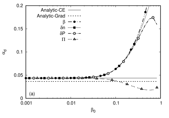
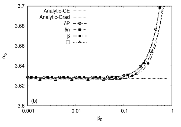
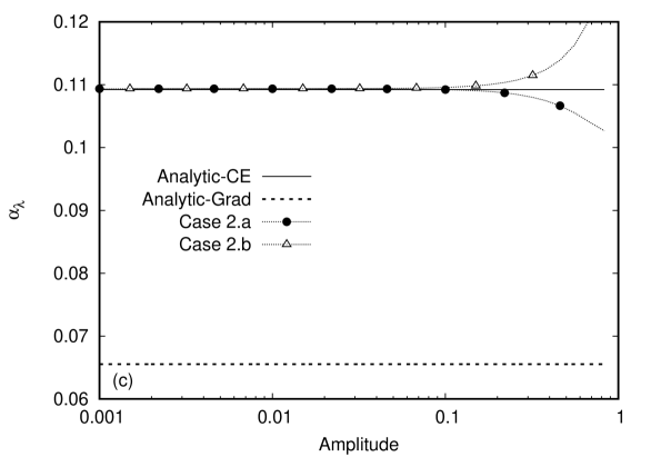
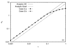
Figure 4: The dependence of (a) ฮฑdsubscript๐›ผ๐‘‘\alpha_{d} and (b) ฮฑosubscript๐›ผ๐‘œ\alpha_{o} on ฮฒ0subscript๐›ฝ0\beta_{0}; the four curves correspond to the two-parameter nonlinear fits of ฮดโ€‹n~~๐›ฟ๐‘›\widetilde{\delta n}, ฮดโ€‹P~~๐›ฟ๐‘ƒ\widetilde{\delta P}, ฮฒ~~๐›ฝ\widetilde{\beta} and ฮ ~~ฮ \widetilde{\Pi} in Eq.ย (43) to the corresponding numerical data, as described in Subsec.ย III.5. (c) The dependence of ฮฑฮปsubscript๐›ผ๐œ†\alpha_{\lambda}, obtained using a nonlinear fit of Eq.ย (44) to the numerical data, on the amplitudes ฮดโ€‹P0๐›ฟsubscript๐‘ƒ0\delta P_{0} (Case 2a) and ฮดโ€‹n0๐›ฟsubscript๐‘›0\delta n_{0} (Case 2b) of the initial perturbation. The relaxation time was always kept at ฯ„=0.0083๐œ0.0083\tau=0.0083.

Next, an assessment of the limits within which the solution of the linearised equations (17) is applicable is performed. In order to reduce the rarefaction effects, ฯ„๐œ\tau is fixed at ฯ„=0.0083๐œ0.0083\tau=0.0083 throughout this subsection.

The solution (43) predicts that, for Case 1, the time evolution of ฮฒ~~๐›ฝ\widetilde{\beta} is damped according to the factor expโก(โˆ’ฮฑdโ€‹t)subscript๐›ผ๐‘‘๐‘ก\exp(-\alpha_{d}t), with ฮฑdsubscript๐›ผ๐‘‘\alpha_{d} (35) being independent of the magnitude ฮฒ0subscript๐›ฝ0\beta_{0} of the perturbation. Figureย 3 shows that this is not the case: while at small values of ฮฒ0subscript๐›ฝ0\beta_{0}, ฮฒ~~๐›ฝ\widetilde{\beta} follows closely the analytic prediction [as confirmed in Fig.ย 1(c)], at larger values of ฮฒ๐›ฝ\beta, the dampening is enhanced compared to the linearised limit (35).

In order to test the versatility of the functional form of the solution corresponding to the linearised regime, the parameters ฮฑdsubscript๐›ผ๐‘‘\alpha_{d}, ฮฑosubscript๐›ผ๐‘œ\alpha_{o} and ฮฑฮปsubscript๐›ผ๐œ†\alpha_{\lambda} are determined using nonlinear fits of the analytic solutions (43) and (44) to the corresponding numerical data. The coefficients ฮฑdsubscript๐›ผ๐‘‘\alpha_{d} and ฮฑosubscript๐›ผ๐‘œ\alpha_{o} are obtained by treating them as free parameters while performing a two-parameter nonlinear fit of ฮดโ€‹n~~๐›ฟ๐‘›\widetilde{\delta n}, ฮฒ~~๐›ฝ\widetilde{\beta}, ฮดโ€‹P~~๐›ฟ๐‘ƒ\widetilde{\delta P} and ฮ ~~ฮ \widetilde{\Pi} given in Eq.ย (43) for the initial conditions corresponding to Case 1 (i.e. ฮดโ€‹n0=ฮดโ€‹P0=0๐›ฟsubscript๐‘›0๐›ฟsubscript๐‘ƒ00\delta n_{0}=\delta P_{0}=0 and various values of ฮฒ0subscript๐›ฝ0\beta_{0}) to the corresponding numerical results. The coefficient ฮฑฮปsubscript๐›ผ๐œ†\alpha_{\lambda} is obtained by performing a one-parameter nonlinear fit of q~~๐‘ž\widetilde{q} with respect to the numerical results with the initial conditions described in Case 2a (ฮฒ0=0subscript๐›ฝ00\beta_{0}=0, ฮดโ€‹n0=0๐›ฟsubscript๐‘›00\delta n_{0}=0 and various values for ฮดโ€‹P0๐›ฟsubscript๐‘ƒ0\delta P_{0}) and Case 2b (ฮฒ0=0subscript๐›ฝ00\beta_{0}=0, ฮดโ€‹P0=0๐›ฟsubscript๐‘ƒ00\delta P_{0}=0 and various values for ฮดโ€‹n0๐›ฟsubscript๐‘›0\delta n_{0}).

The dependence of ฮฑdsubscript๐›ผ๐‘‘\alpha_{d}, ฮฑosubscript๐›ผ๐‘œ\alpha_{o} and ฮฑฮปsubscript๐›ผ๐œ†\alpha_{\lambda} on the amplitude of the perturbations is presented in the plots (a), (b) and (c) of Fig.ย 4, respectively. The horizontal axis in Fig.ย 4(c) represents the amplitude of the initial perturbation, i.e. ฮดโ€‹P0๐›ฟsubscript๐‘ƒ0\delta P_{0} for Case 2a and ฮดโ€‹n0๐›ฟsubscript๐‘›0\delta n_{0} for Case 2b. All of the above plots show the analytic predictions (35) and (31) for ฮฑdsubscript๐›ผ๐‘‘\alpha_{d}, ฮฑosubscript๐›ผ๐‘œ\alpha_{o} and ฮฑฮปsubscript๐›ผ๐œ†\alpha_{\lambda}, specialised to the cases when the transport coefficients ฮท๐œ‚\eta and ฮป๐œ†\lambda are computed using the Chapman-Enskog (26b) and the Grad (26a) expressions. The results clearly favor the Chapman-Enskog expressions. These plots also indicate that the analytic analysis performed in Sec.ย III.2 in the context of the linearised hydrodynamic equations loses applicability when the perturbation amplitudes ฮฒ0subscript๐›ฝ0\beta_{0}, ฮดโ€‹n0/n0๐›ฟsubscript๐‘›0subscript๐‘›0\delta n_{0}/n_{0} or ฮดโ€‹P0/P0๐›ฟsubscript๐‘ƒ0subscript๐‘ƒ0\delta P_{0}/P_{0} are larger than โˆผ0.05similar-toabsent0.05\sim 0.05.

III.6 Limits of the first-order hydrodynamics regime
Refer to caption Refer to caption
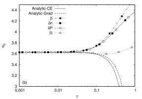
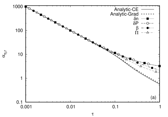
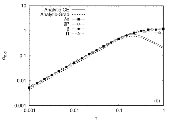
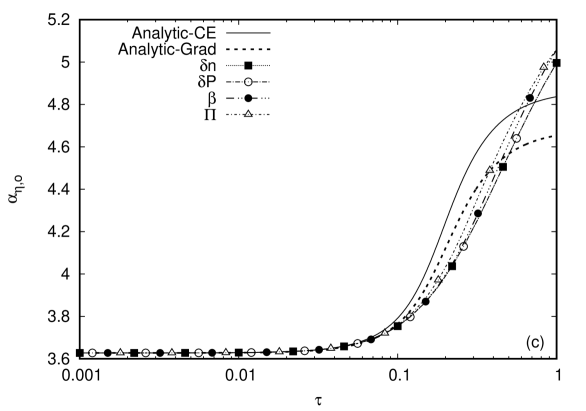
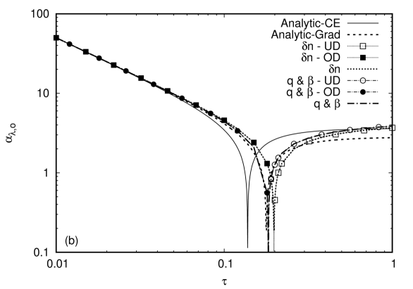
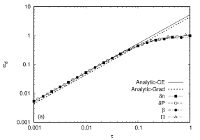
Figure 5: Graphical representation of the dependence on ฯ„๐œ\tau of (a) ฮฑdsubscript๐›ผ๐‘‘\alpha_{d}, (b) ฮฑosubscript๐›ผ๐‘œ\alpha_{o} and (c) ฮฑฮปsubscript๐›ผ๐œ†\alpha_{\lambda} obtained using the nonlinear fitting procedure described in Subsec.ย III.5. In (d), the ratio ฮฑฮป/ฮฑdsubscript๐›ผ๐œ†subscript๐›ผ๐‘‘\alpha_{\lambda}/\alpha_{d} is represented with respect to ฯ„๐œ\tau, where ฮฑdsubscript๐›ผ๐‘‘\alpha_{d} is obtained using the two-parameter nonlinear fit of ฮฒ~~๐›ฝ\widetilde{\beta} (43) on the numerical data, while ฮฑฮปsubscript๐›ผ๐œ†\alpha_{\lambda} is obtained using a one-parameter nonlinear fit of q~~๐‘ž\widetilde{q} (44) for Case 2a. The perturbation amplitude is in all cases set to 10โˆ’3superscript10310^{-3}. On each plot, the analytic curves corresponding to the Chapman-Enskog and Grad methods are displayed.

It is known that the constitutive equations (7) are valid only when ฯ„๐œ\tau is small cercignani02 . This subsection is focused on investigating the validity of the analysis presented in Sec.ย III.2 as the relaxation time ฯ„๐œ\tau is increased.

In order to test the effect of increasing ฯ„๐œ\tau, the perturbations are kept at a small value, i.e. ฮฒ0=10โˆ’3subscript๐›ฝ0superscript103\beta_{0}=10^{-3} (for Case 1), ฮดโ€‹P0=10โˆ’3๐›ฟsubscript๐‘ƒ0superscript103\delta P_{0}=10^{-3} (for Case 2a), or ฮดโ€‹n0=10โˆ’3๐›ฟsubscript๐‘›0superscript103\delta n_{0}=10^{-3} (for Case 2b). The plots in Fig.ย 5 show the dependence of (a) ฮฑdsubscript๐›ผ๐‘‘\alpha_{d}, (b) ฮฑosubscript๐›ผ๐‘œ\alpha_{o}, (c) ฮฑฮปsubscript๐›ผ๐œ†\alpha_{\lambda} and (d) the ratio ฮป/ฮท=2โ€‹ฮฑฮปโ€‹n0/3โ€‹ฮฑdโ€‹P0๐œ†๐œ‚2subscript๐›ผ๐œ†subscript๐‘›03subscript๐›ผ๐‘‘subscript๐‘ƒ0\lambda/\eta=2\alpha_{\lambda}n_{0}/3\alpha_{d}P_{0} on the value of ฯ„๐œ\tau. As before, the analytic predictions for the dependence of these coefficients on ฯ„๐œ\tau is also shown for the cases when the transport coefficients ฮท๐œ‚\eta and ฮป๐œ†\lambda are obtained using the Chapman-Enskog (26b) and Grad (26a) expressions. For ฯ„<0.1๐œ0.1\tau<0.1, the numerical results clearly favor the Chapman-Enskog expression. Plot (d) confirms that for small values of ฯ„๐œ\tau, the ratio ฮป/ฮท๐œ†๐œ‚\lambda/\eta is equal to 5/3535/3, as predicted in the Chapman-Enskog theory (26b). This value is in agreement with the high chemical potential limit of Fig.ย 2 in Ref.ย jaiswal15 .

While for ฯ„โ‰ณ0.1greater-than-or-equivalent-to๐œ0.1\tau\gtrsim 0.1, the constitutive equations (7) no longer hold, our nonlinear fit analysis seems to indicate that the dampening coefficients ฮฑdsubscript๐›ผ๐‘‘\alpha_{d} and ฮฑฮปsubscript๐›ผ๐œ†\alpha_{\lambda} plateau at large ฯ„๐œ\tau. This conclusion is not necessarily meaningful, since the ansatz (20) that the time dependence of ฮดโ€‹n๐›ฟ๐‘›\delta n, ฮดโ€‹P๐›ฟ๐‘ƒ\delta P and ฮฒ๐›ฝ\beta is of the form eโˆ’ฮฑโ€‹tsuperscript๐‘’๐›ผ๐‘กe^{-\alpha t} with constant ฮฑ๐›ผ\alpha is not guaranteed to be valid in the transition regime. It is certain that the time dependence of the above quantities is more complex at large values of ฯ„๐œ\tau, since the dissipative exponential attenuation is replaced by a polynomial dispersive attenuation in the ballistic regime, as will be shown in Sec.ย VI.

III.7 Summary

In this section, the attenuation of a longitudinal wave was analysed using the equations of first-order hydrodynamics. The results obtained by numerically solving the AWB equation at small values of the relaxation time ฯ„๐œ\tau showed an excellent agreement with the analytic results when the transport coefficinets ฮป๐œ†\lambda and ฮท๐œ‚\eta were obtained using the Chapman-Enskog method. The analytic results corresponding to the transport coefficients obtained using the Grad method exhibited a clear discrepancy compared to the numerical results.

The validity of the linearised form of the AWB equation (18) was further tested by comparing the numerical and analytic results at increasing values of the wave amplitudes, while keeping ฯ„=0.0083๐œ0.0083\tau=0.0083. A visible discrepancy can be seen at wave amplitudes of ฮฒ0,ฮดโ€‹n0/n0,ฮดโ€‹P0/P0โ‰ณ0.1greater-than-or-equivalent-tosubscript๐›ฝ0๐›ฟsubscript๐‘›0subscript๐‘›0๐›ฟsubscript๐‘ƒ0subscript๐‘ƒ00.1\beta_{0},\delta n_{0}/n_{0},\delta P_{0}/P_{0}\gtrsim 0.1. The applicability of the functional form of the solution of the first-order hydrodynamics equations was further considered by numerically fitting the attenuation coefficients ฮฑฮปsubscript๐›ผ๐œ†\alpha_{\lambda} and ฮฑฮทsubscript๐›ผ๐œ‚\alpha_{\eta}, as well as the oscillation frequency ฮฑosubscript๐›ผ๐‘œ\alpha_{o}, to the numerical results. The above analysis shows that the best fit parameters differ significantly from the analytic prediction when the wave amplitude is โ‰ณ0.05greater-than-or-equivalent-toabsent0.05\gtrsim 0.05. At smaller values of the wave amplitudes, the numerical results clearly favored the Chapman-Enskog predictions for the transport coefficients, while the Grad predictions showed a visible discrepancy to the numerical results.

Finally, the validity of the first-order hydrodynamics equations was investigated at increasing values of ฯ„๐œ\tau. The dampening coefficients ฮฑdsubscript๐›ผ๐‘‘\alpha_{d} and ฮฑฮปsubscript๐›ผ๐œ†\alpha_{\lambda} were found to be directly proportional to ฯ„๐œ\tau only for ฯ„โ‰ฒ0.1less-than-or-similar-to๐œ0.1\tau\lesssim 0.1, confirming the Chapman-Enskog prediction. At larger values of ฯ„๐œ\tau, they increase at a significantly slower rate, signaling the breakdown of the first-order hydrodynamics formulation when ฯ„โ‰ณ0.1greater-than-or-equivalent-to๐œ0.1\tau\gtrsim 0.1. The Grad prediction was in clear disagreement with the numerical results for all values of ฯ„๐œ\tau.

IV Second-order hydrodynamics

The five-field theory provides the constitutive equations for qฮผsuperscript๐‘ž๐œ‡q^{\mu} and ฮ ฮผโ€‹ฮฝsuperscriptฮ ๐œ‡๐œˆ\Pi^{\mu\nu} in the form given in Eq.ย (24). Since these constitutive equations do not represent evolution equations, qฮผsuperscript๐‘ž๐œ‡q^{\mu} and ฮ ฮผโ€‹ฮฝsuperscriptฮ ๐œ‡๐œˆ\Pi^{\mu\nu} are fully determined by the spatial and temporal gradients of n๐‘›n, uฮผsuperscript๐‘ข๐œ‡u^{\mu} and P๐‘ƒP. In particular, their initial values at t=0๐‘ก0t=0 cannot be set to arbitrary values. In this section, the second-order extension of the five-field theory will be employed in order to study the relaxation process of the heat flux and shear stress from their initial vanishing value to the value required through the constitutive equations of the five-field theory.

IV.1 Constitutive relations

There are many variations of the form in which the equations of second-order hydrodynamics (also known as extended irreversible thermodynamics rezzolla13 ) are presented, essentially due to the route adopted in deriving them israel79 ; hiscock83 ; el10 ; denicol10 ; jaiswal13b ; chattopadhyay15 . Only the form introduced in Refs.ย hiscock83 ; rezzolla13 will be further considered, according to which qฮผsuperscript๐‘ž๐œ‡q^{\mu} and Tฮผโ€‹ฮฝsuperscript๐‘‡๐œ‡๐œˆT^{\mu\nu} satisfy the following equations:

qฮผ=superscript๐‘ž๐œ‡absent\displaystyle q^{\mu}= โˆ’ฮปTฮ”ฮผโ€‹ฮฝ[โˆ‚ฮฝlnT+uฯโˆ‚ฯuฮฝ+ฮฒ1uฯโˆ‚ฯqฮฝโˆ’ฮฑ1โˆ‚ฯฮ ฯโˆ’ฮฝ(1โˆ’ฮณ1)Tฮ ฯโˆ‚ฯฮฝ(ฮฑ1T)+12Tqฮฝโˆ‚ฯ(ฮฒ1โ€‹uฯT)],\displaystyle-\lambda T\Delta^{\mu\nu}\Bigg{[}\partial_{\nu}\ln T+u^{\rho}\partial_{\rho}u_{\nu}+\beta_{1}u^{\rho}\partial_{\rho}q_{\nu}-\alpha_{1}\partial_{\rho}\Pi^{\rho}{}_{\nu}-(1-\gamma_{1})T\Pi^{\rho}{}_{\nu}\partial_{\rho}\left(\frac{\alpha_{1}}{T}\right)+\frac{1}{2}Tq_{\nu}\partial_{\rho}\left(\frac{\beta_{1}u^{\rho}}{T}\right)\Bigg{]},
ฮ ฮผโ€‹ฮฝ=superscriptฮ ๐œ‡๐œˆabsent\displaystyle\Pi^{\mu\nu}= โˆ’2โ€‹ฮทโ€‹[12โ€‹(ฮ”ฮผโ€‹ฮปโ€‹ฮ”ฮฝโ€‹ฮบ+ฮ”ฮฝโ€‹ฮปโ€‹ฮ”ฮผโ€‹ฮบ)โˆ’13โ€‹ฮ”ฮผโ€‹ฮฝโ€‹ฮ”ฮปโ€‹ฮบ]2๐œ‚delimited-[]12superscriptฮ”๐œ‡๐œ†superscriptฮ”๐œˆ๐œ…superscriptฮ”๐œˆ๐œ†superscriptฮ”๐œ‡๐œ…13superscriptฮ”๐œ‡๐œˆsuperscriptฮ”๐œ†๐œ…\displaystyle-2\eta\left[\frac{1}{2}\left(\Delta^{\mu\lambda}\Delta^{\nu\kappa}+\Delta^{\nu\lambda}\Delta^{\mu\kappa}\right)-\frac{1}{3}\Delta^{\mu\nu}\Delta^{\lambda\kappa}\right]
ร—[โˆ‚ฮปuฮบ+ฮฒ2โ€‹uฯโ€‹โˆ‚ฯฮ ฮปโ€‹ฮบโˆ’ฮฑ1โ€‹โˆ‚ฮปqฮบโˆ’ฮณ1โ€‹Tโ€‹qฮปโ€‹โˆ‚ฮบ(ฮฑ1T)+12โ€‹Tโ€‹ฮ ฮปโ€‹ฮบโ€‹โˆ‚ฯ(ฮฒ2Tโ€‹uฯ)],absentdelimited-[]subscript๐œ†subscript๐‘ข๐œ…subscript๐›ฝ2superscript๐‘ข๐œŒsubscript๐œŒsubscriptฮ ๐œ†๐œ…subscript๐›ผ1subscript๐œ†subscript๐‘ž๐œ…subscript๐›พ1๐‘‡subscript๐‘ž๐œ†subscript๐œ…subscript๐›ผ1๐‘‡12๐‘‡subscriptฮ ๐œ†๐œ…subscript๐œŒsubscript๐›ฝ2๐‘‡superscript๐‘ข๐œŒ\displaystyle\times\left[\partial_{\lambda}u_{\kappa}+\beta_{2}u^{\rho}\partial_{\rho}\Pi_{\lambda\kappa}-\alpha_{1}\partial_{\lambda}q_{\kappa}-\gamma_{1}Tq_{\lambda}\partial_{\kappa}\left(\frac{\alpha_{1}}{T}\right)+\frac{1}{2}T\Pi_{\lambda\kappa}\partial_{\rho}\left(\frac{\beta_{2}}{T}u^{\rho}\right)\right], (45)

where the thermodynamic coefficients ฮฒ1subscript๐›ฝ1\beta_{1}, ฮฒ2subscript๐›ฝ2\beta_{2} and ฮณ1subscript๐›พ1\gamma_{1} and the viscous-heat flux coupling coefficient ฮฑ1subscript๐›ผ1\alpha_{1} are a priori not known. After performing the linearisation described in Sec.ย II.2, Eq.ย (45) becomes:

ฯ„qโ€‹โˆ‚tq+q=subscript๐œ๐‘žsubscript๐‘ก๐‘ž๐‘žabsent\displaystyle\tau_{q}\partial_{t}q+q= โˆ’ฮปโ€‹P04โ€‹n0โ€‹(3โ€‹โˆ‚zฮดโ€‹PP0โˆ’4โ€‹โˆ‚zฮดโ€‹nn0)+ฮป4โ€‹n0โ€‹(1+4โ€‹ฮฑ1โ€‹P0)โ€‹โˆ‚zฮ ,๐œ†subscript๐‘ƒ04subscript๐‘›03subscript๐‘ง๐›ฟ๐‘ƒsubscript๐‘ƒ04subscript๐‘ง๐›ฟ๐‘›subscript๐‘›0๐œ†4subscript๐‘›014subscript๐›ผ1subscript๐‘ƒ0subscript๐‘งฮ \displaystyle-\frac{\lambda P_{0}}{4n_{0}}\left(\frac{3\partial_{z}\delta P}{P_{0}}-\frac{4\partial_{z}\delta n}{n_{0}}\right)+\frac{\lambda}{4n_{0}}(1+4\alpha_{1}P_{0})\partial_{z}\Pi, (46a)
ฯ„ฮ โ€‹โˆ‚tฮ +ฮ =subscript๐œฮ subscript๐‘กฮ ฮ absent\displaystyle\tau_{\Pi}\partial_{t}\Pi+\Pi= โˆ’4โ€‹ฮท3โ€‹โˆ‚z(ฮฒโˆ’ฮฑ1โ€‹q),4๐œ‚3subscript๐‘ง๐›ฝsubscript๐›ผ1๐‘ž\displaystyle-\frac{4\eta}{3}\partial_{z}\left(\beta-\alpha_{1}q\right), (46b)

where Eq.ย (17) was used to eliminate the time derivative of ฮฒ๐›ฝ\beta in Eq.ย (46a), while the relaxation times were defined as ฯ„q=ฮปโ€‹(Tโ€‹ฮฒ1โˆ’1/4โ€‹n0)subscript๐œ๐‘ž๐œ†๐‘‡subscript๐›ฝ114subscript๐‘›0\tau_{q}=\lambda(T\beta_{1}-1/4n_{0}) and ฯ„ฮ =2โ€‹ฮทโ€‹ฮฒ2subscript๐œฮ 2๐œ‚subscript๐›ฝ2\tau_{\Pi}=2\eta\beta_{2}. In order for the constitutive equation for q๐‘žq and ฮ ฮ \Pi to match the first-order versions (27) in the limit ฯ„q,ฯ„ฮ โ†’0โ†’subscript๐œ๐‘žsubscript๐œฮ 0\tau_{q},\tau_{\Pi}\rightarrow 0, we set ฮฑ1=โˆ’1/4โ€‹P0subscript๐›ผ114subscript๐‘ƒ0\alpha_{1}=-1/4P_{0} and Eqs.ย (46) reduce to:

ฯ„qโ€‹โˆ‚tq+q=subscript๐œ๐‘žsubscript๐‘ก๐‘ž๐‘žabsent\displaystyle\tau_{q}\partial_{t}q+q= โˆ’ฮปโ€‹P04โ€‹n0โ€‹(3โ€‹โˆ‚zฮดโ€‹PP0โˆ’4โ€‹โˆ‚zฮดโ€‹nn0),๐œ†subscript๐‘ƒ04subscript๐‘›03subscript๐‘ง๐›ฟ๐‘ƒsubscript๐‘ƒ04subscript๐‘ง๐›ฟ๐‘›subscript๐‘›0\displaystyle-\frac{\lambda P_{0}}{4n_{0}}\left(\frac{3\partial_{z}\delta P}{P_{0}}-\frac{4\partial_{z}\delta n}{n_{0}}\right), (47a)
ฯ„ฮ โ€‹โˆ‚tฮ +ฮ =subscript๐œฮ subscript๐‘กฮ ฮ absent\displaystyle\tau_{\Pi}\partial_{t}\Pi+\Pi= โˆ’4โ€‹ฮท3โ€‹โˆ‚z(ฮฒ+q4โ€‹P0),4๐œ‚3subscript๐‘ง๐›ฝ๐‘ž4subscript๐‘ƒ0\displaystyle-\frac{4\eta}{3}\partial_{z}\left(\beta+\frac{q}{4P_{0}}\right), (47b)

By analogy to Eq.ย (25), the reduced relaxation times ฯ„q,0subscript๐œ๐‘ž0\tau_{q,0} and ฯ„ฮ ,0subscript๐œฮ 0\tau_{\Pi,0} can be introduced through:

ฯ„q=ฯ„q,0โ€‹ฯ„,ฯ„ฮ =ฯ„ฮ ,0โ€‹ฯ„.formulae-sequencesubscript๐œ๐‘žsubscript๐œ๐‘ž0๐œsubscript๐œฮ subscript๐œฮ 0๐œ\tau_{q}=\tau_{q,0}\tau,\qquad\tau_{\Pi}=\tau_{\Pi,0}\tau. (48)

In general, the values of ฯ„q,0subscript๐œ๐‘ž0\tau_{q,0} and ฯ„ฮ ,0subscript๐œฮ 0\tau_{\Pi,0} are determined by the properties of the collision term in the Boltzmann equation. When the Anderson-Witting single relaxation time approximation is used, the following values for ฯ„q,0subscript๐œ๐‘ž0\tau_{q,0} and ฯ„ฮ ,0subscript๐œฮ 0\tau_{\Pi,0} are commonly employed within both the Chapman-Enskog- and moment-like methods denicol12 ; jaiswal13a ; bhalerao14 ; chattopadhyay15 ; tinti17 :

ฯ„ฮ ,0=1,ฯ„q,0=1.formulae-sequencesubscript๐œฮ 01subscript๐œ๐‘ž01\tau_{\Pi,0}=1,\qquad\tau_{q,0}=1. (49)

It is interesting to test the hyperbolicity of the resulting set of equations. Equations (17) and (47) can be written in the following form:

โˆ‚t๐•Œ+โˆ‚z(๐”ธโ€‹๐•Œ)=๐•Š,subscript๐‘ก๐•Œsubscript๐‘ง๐”ธ๐•Œ๐•Š\partial_{t}\mathbb{U}+\partial_{z}(\mathbb{A}\mathbb{U})=\mathbb{S}, (50)

where

๐•Œ=๐•Œabsent\displaystyle\mathbb{U}= (ฮดโ€‹nn0,ฮดโ€‹PP0,ฮฒ,qP0,ฮ P0)T,superscript๐›ฟ๐‘›subscript๐‘›0๐›ฟ๐‘ƒsubscript๐‘ƒ0๐›ฝ๐‘žsubscript๐‘ƒ0ฮ subscript๐‘ƒ0๐‘‡\displaystyle\left(\frac{\delta n}{n_{0}},\frac{\delta P}{P_{0}},\beta,\frac{q}{P_{0}},\frac{\Pi}{P_{0}}\right)^{T},
๐•Š=๐•Šabsent\displaystyle\mathbb{S}= (0,0,q4โ€‹ฯ„qโ€‹P0,โˆ’qฯ„qโ€‹P0,โˆ’ฮ ฯ„ฮ โ€‹P0)T,superscript00๐‘ž4subscript๐œ๐‘žsubscript๐‘ƒ0๐‘žsubscript๐œ๐‘žsubscript๐‘ƒ0ฮ subscript๐œฮ subscript๐‘ƒ0๐‘‡\displaystyle\left(0,0,\frac{q}{4\tau_{q}P_{0}},-\frac{q}{\tau_{q}P_{0}},-\frac{\Pi}{\tau_{\Pi}P_{0}}\right)^{T}, (51)

while ๐”ธ๐”ธ\mathbb{A} is given by:

๐”ธ=(001000043130ฮป04โ€‹ฯ„q,014โˆ’3โ€‹ฮป016โ€‹ฯ„q,00014โˆ’ฮป0ฯ„q,03โ€‹ฮป04โ€‹ฯ„q,0000004โ€‹ฮท03โ€‹ฯ„ฮ ,0ฮท03โ€‹ฯ„ฮ ,00).๐”ธmatrix001000043130subscript๐œ†04subscript๐œ๐‘ž0143subscript๐œ†016subscript๐œ๐‘ž00014subscript๐œ†0subscript๐œ๐‘ž03subscript๐œ†04subscript๐œ๐‘ž0000004subscript๐œ‚03subscript๐œฮ 0subscript๐œ‚03subscript๐œฮ 00\mathbb{A}=\begin{pmatrix}0&0&1&0&0\\ 0&0&\frac{4}{3}&\frac{1}{3}&0\\ \frac{\lambda_{0}}{4\tau_{q,0}}&\frac{1}{4}-\frac{3\lambda_{0}}{16\tau_{q,0}}&0&0&\frac{1}{4}\\ -\frac{\lambda_{0}}{\tau_{q,0}}&\frac{3\lambda_{0}}{4\tau_{q,0}}&0&0&0\\ 0&0&\frac{4\eta_{0}}{3\tau_{\Pi,0}}&\frac{\eta_{0}}{3\tau_{\Pi,0}}&0\end{pmatrix}. (52)

The five eigenvalues of ๐”ธ๐”ธ\mathbb{A} can be found analytically and are given by a0=0subscript๐‘Ž00a_{0}=0 and

aฮป,ยฑ=ยฑ12โ€‹ฮป0ฯ„q,0,aฮท,ยฑ=ยฑ13โ€‹1+ฮท0ฯ„ฮ ,0.formulae-sequencesubscript๐‘Ž๐œ†plus-or-minusplus-or-minus12subscript๐œ†0subscript๐œ๐‘ž0subscript๐‘Ž๐œ‚plus-or-minusplus-or-minus131subscript๐œ‚0subscript๐œฮ 0a_{\lambda,\pm}=\pm\frac{1}{2}\sqrt{\frac{\lambda_{0}}{\tau_{q,0}}},\qquad a_{\eta,\pm}=\pm\frac{1}{\sqrt{3}}\sqrt{1+\frac{\eta_{0}}{\tau_{\Pi,0}}}. (53)

Since the eigenvalues of ๐”ธ๐”ธ\mathbb{A} are real, the system of equations (50) is hyperbolic rezzolla13 ; toro09 .

IV.2 Longitudinal waves: modes

Employing the ansรคtze (20) and (21) allows ฮ ฮฑsubscriptฮ ๐›ผ\Pi_{\alpha} to be expressed from Eq.ย (47b) as follows:

ฮ ฮฑ=โˆ’4โ€‹kโ€‹ฮท3โ€‹(1โˆ’ฮฑโ€‹ฯ„ฮ )โ€‹(ฮฒฮฑ+qฮฑ4โ€‹P0).subscriptฮ ๐›ผ4๐‘˜๐œ‚31๐›ผsubscript๐œฮ subscript๐›ฝ๐›ผsubscript๐‘ž๐›ผ4subscript๐‘ƒ0\Pi_{\alpha}=-\frac{4k\eta}{3(1-\alpha\tau_{\Pi})}\left(\beta_{\alpha}+\frac{q_{\alpha}}{4P_{0}}\right). (54)

Furthermore, Eq.ย (22b) allows ฮดโ€‹Pฮฑ๐›ฟsubscript๐‘ƒ๐›ผ\delta P_{\alpha} to be written as:

ฮดโ€‹Pฮฑ=4โ€‹kโ€‹P03โ€‹ฮฑโ€‹(ฮฒฮฑ+qฮฑ4โ€‹P0).๐›ฟsubscript๐‘ƒ๐›ผ4๐‘˜subscript๐‘ƒ03๐›ผsubscript๐›ฝ๐›ผsubscript๐‘ž๐›ผ4subscript๐‘ƒ0\delta P_{\alpha}=\frac{4kP_{0}}{3\alpha}\left(\beta_{\alpha}+\frac{q_{\alpha}}{4P_{0}}\right). (55)

Inserting Eq.ย (54) and (55) into Eq.ย (22c) yields:

[ฮฑ+k23โ€‹ฮฑโˆ’ฮทโ€‹k23โ€‹P0โ€‹(1โˆ’ฮฑโ€‹ฯ„ฮ )]โ€‹(ฮฒฮฑ+qฮฑ4โ€‹P0)=0.delimited-[]๐›ผsuperscript๐‘˜23๐›ผ๐œ‚superscript๐‘˜23subscript๐‘ƒ01๐›ผsubscript๐œฮ subscript๐›ฝ๐›ผsubscript๐‘ž๐›ผ4subscript๐‘ƒ00\left[\alpha+\frac{k^{2}}{3\alpha}-\frac{\eta k^{2}}{3P_{0}(1-\alpha\tau_{\Pi})}\right]\left(\beta_{\alpha}+\frac{q_{\alpha}}{4P_{0}}\right)=0. (56)

The above equation is satisfied when either of the two factors cancel. These two cases are discussed separately below.

qฮฑ=โˆ’4โ€‹P0โ€‹ฮฒฮฑsubscript๐‘ž๐›ผ4subscript๐‘ƒ0subscript๐›ฝ๐›ผq_{\alpha}=-4P_{0}\beta_{\alpha}.

This case is also recovered for qฮปsubscript๐‘ž๐œ†q_{\lambda} in the first-order approximation (32). In this case, Eqs.ย (54) and (55) show that ฮ ฮฑ=ฮดโ€‹Pฮฑ=0subscriptฮ ๐›ผ๐›ฟsubscript๐‘ƒ๐›ผ0\Pi_{\alpha}=\delta P_{\alpha}=0. The values of ฮฑ๐›ผ\alpha corresponding to this regime can be found from Eq.ย (47a), which reduces to:

[ฮปโ€‹k2ฮฑโ€‹n0โˆ’4โ€‹(1โˆ’ฮฑโ€‹ฯ„q)]โ€‹ฮฒฮฑ=0.delimited-[]๐œ†superscript๐‘˜2๐›ผsubscript๐‘›041๐›ผsubscript๐œ๐‘žsubscript๐›ฝ๐›ผ0\left[\frac{\lambda k^{2}}{\alpha n_{0}}-4(1-\alpha\tau_{q})\right]\beta_{\alpha}=0. (57)

The case ฮฒฮฑ=0subscript๐›ฝ๐›ผ0\beta_{\alpha}=0 trivially corresponds to a vanishing perturbation (i.e. ฮดโ€‹nฮฑ=ฮดโ€‹Pฮฑ=0๐›ฟsubscript๐‘›๐›ผ๐›ฟsubscript๐‘ƒ๐›ผ0\delta n_{\alpha}=\delta P_{\alpha}=0). Setting the term inside the square bracket to 00 yields the following values for ฮฑ๐›ผ\alpha:

ฮฑฮป,+=subscript๐›ผ๐œ†absent\displaystyle\alpha_{\lambda,+}= 12โ€‹ฯ„qโ€‹(1+1โˆ’k2โ€‹ฮปโ€‹ฯ„qn0)โ‰ƒ1ฯ„qโˆ’ฮฑฮป+Oโ€‹(ฯ„3),similar-to-or-equals12subscript๐œ๐‘ž11superscript๐‘˜2๐œ†subscript๐œ๐‘žsubscript๐‘›01subscript๐œ๐‘žsubscript๐›ผ๐œ†๐‘‚superscript๐œ3\displaystyle\frac{1}{2\tau_{q}}\left(1+\sqrt{1-\frac{k^{2}\lambda\tau_{q}}{n_{0}}}\right)\simeq\frac{1}{\tau_{q}}-\alpha_{\lambda}+O(\tau^{3}),
ฮฑฮป,โˆ’=subscript๐›ผ๐œ†absent\displaystyle\alpha_{\lambda,-}= 12โ€‹ฯ„qโ€‹(1โˆ’1โˆ’k2โ€‹ฮปโ€‹ฯ„qn0)โ‰ƒฮฑฮป+Oโ€‹(ฯ„3).similar-to-or-equals12subscript๐œ๐‘ž11superscript๐‘˜2๐œ†subscript๐œ๐‘žsubscript๐‘›0subscript๐›ผ๐œ†๐‘‚superscript๐œ3\displaystyle\frac{1}{2\tau_{q}}\left(1-\sqrt{1-\frac{k^{2}\lambda\tau_{q}}{n_{0}}}\right)\simeq\alpha_{\lambda}+O(\tau^{3}). (58)

It can be seen that, in the small ฯ„๐œ\tau limit, ฮฑฮป,โˆ’subscript๐›ผ๐œ†\alpha_{\lambda,-} corresponds to the dampening coefficient ฮฑฮป=k2โ€‹ฮป/4โ€‹n0subscript๐›ผ๐œ†superscript๐‘˜2๐œ†4subscript๐‘›0\alpha_{\lambda}=k^{2}\lambda/4n_{0} identified in the first-order theory (31). The term ฮฑฮป,+subscript๐›ผ๐œ†\alpha_{\lambda,+} allows q~~๐‘ž\widetilde{q} to relax from an arbitrary initial condition at t=0๐‘ก0t=0 to the first-order expression (27) on a timescale of order ฯ„qsubscript๐œ๐‘ž\tau_{q}. The modes corresponding to the above values of ฮฑฮป,ยฑsubscript๐›ผ๐œ†plus-or-minus\alpha_{\lambda,\pm} can be written in terms of the amplitudes ฮฒฮป,ยฑsubscript๐›ฝ๐œ†plus-or-minus\beta_{\lambda,\pm} as follows:

ฮดโ€‹nฮป,ยฑ=kโ€‹n0ฮฑฮป,ยฑโ€‹ฮฒฮป,ยฑ,qฮป,ยฑ=โˆ’4โ€‹P0โ€‹ฮฒฮป,ยฑ,formulae-sequence๐›ฟsubscript๐‘›๐œ†plus-or-minus๐‘˜subscript๐‘›0subscript๐›ผ๐œ†plus-or-minussubscript๐›ฝ๐œ†plus-or-minussubscript๐‘ž๐œ†plus-or-minus4subscript๐‘ƒ0subscript๐›ฝ๐œ†plus-or-minus\displaystyle\delta n_{\lambda,\pm}=\frac{kn_{0}}{\alpha_{\lambda,\pm}}\beta_{\lambda,\pm},\qquad q_{\lambda,\pm}=-4P_{0}\beta_{\lambda,\pm},
ฮดโ€‹Pฮป,ยฑ=ฮ ฮป,ยฑ=0.๐›ฟsubscript๐‘ƒ๐œ†plus-or-minussubscriptฮ ๐œ†plus-or-minus0\displaystyle\delta P_{\lambda,\pm}=\Pi_{\lambda,\pm}=0. (59)

The square root in the definition of ฮฑฮป,ยฑsubscript๐›ผ๐œ†plus-or-minus\alpha_{\lambda,\pm} (58) becomes imaginary when ฯ„>ฯ„ฮป,lim๐œsubscript๐œ๐œ†lim\tau>\tau_{\lambda,{\rm lim}}, where

ฯ„ฮป,lim=1kโ€‹ฯ„q,0โ€‹ฮป0.subscript๐œ๐œ†lim1๐‘˜subscript๐œ๐‘ž0subscript๐œ†0\tau_{\lambda,{\rm lim}}=\frac{1}{k\sqrt{\tau_{q,0}\lambda_{0}}}. (60)

When 0<ฯ„<ฯ„ฮป,lim0๐œsubscript๐œ๐œ†lim0<\tau<\tau_{\lambda,{\rm lim}}, the modes corresponding to ฮฑฮป,ยฑsubscript๐›ผ๐œ†plus-or-minus\alpha_{\lambda,\pm} are overdamped (evanescent), while when ฯ„>ฯ„ฮป,lim๐œsubscript๐œ๐œ†lim\tau>\tau_{\lambda,{\rm lim}}, the underdamped regime settles in. In order to treat both regimes within a unitary framework, it is convenient to cast Eq.ย (58) in the form ฮฑฮป,ยฑ=ฮฑฮป,dยฑฮฑฮป,o=ฮฑฮป,dยฑiโ€‹ฮฑยฏฮป,osubscript๐›ผ๐œ†plus-or-minusplus-or-minussubscript๐›ผ๐œ†๐‘‘subscript๐›ผ๐œ†๐‘œplus-or-minussubscript๐›ผ๐œ†๐‘‘๐‘–subscriptยฏ๐›ผ๐œ†๐‘œ\alpha_{\lambda,\pm}=\alpha_{\lambda,d}\pm\alpha_{\lambda,o}=\alpha_{\lambda,d}\pm i\overline{\alpha}_{\lambda,o}, where ฮฑฮป,d=1/2โ€‹ฯ„qsubscript๐›ผ๐œ†๐‘‘12subscript๐œ๐‘ž\alpha_{\lambda,d}=1/2\tau_{q} and

ฮฑฮป,o=subscript๐›ผ๐œ†๐‘œabsent\displaystyle\alpha_{\lambda,o}= ฮฑฮป,dโ€‹1โˆ’k2โ€‹ฮปโ€‹ฯ„qn0,subscript๐›ผ๐œ†๐‘‘1superscript๐‘˜2๐œ†subscript๐œ๐‘žsubscript๐‘›0\displaystyle\alpha_{\lambda,d}\sqrt{1-\frac{k^{2}\lambda\tau_{q}}{n_{0}}},
ฮฑยฏฮป,o=subscriptยฏ๐›ผ๐œ†๐‘œabsent\displaystyle\overline{\alpha}_{\lambda,o}= ฮฑฮป,dโ€‹k2โ€‹ฮปโ€‹ฯ„qn0โˆ’1.subscript๐›ผ๐œ†๐‘‘superscript๐‘˜2๐œ†subscript๐œ๐‘žsubscript๐‘›01\displaystyle\alpha_{\lambda,d}\sqrt{\frac{k^{2}\lambda\tau_{q}}{n_{0}}-1}. (61)

qฮฑ=0subscript๐‘ž๐›ผ0q_{\alpha}=0.

Next, the case when the first bracket in Eq.ย (56) vanishes is considered. Substituting Eqs.ย (22a) and (55) in Eq.ย (47a) yields:

[ฮปโ€‹k2ฮฑโ€‹n0โˆ’4โ€‹(1โˆ’ฮฑโ€‹ฯ„q)]โ€‹qฮฑ=0.delimited-[]๐œ†superscript๐‘˜2๐›ผsubscript๐‘›041๐›ผsubscript๐œ๐‘žsubscript๐‘ž๐›ผ0\left[\frac{\lambda k^{2}}{\alpha n_{0}}-4(1-\alpha\tau_{q})\right]q_{\alpha}=0. (62)

The term inside the square bracket is identical to the one in Eq.ย (57). Setting this term to 00 yields the same values for ฮฑ๐›ผ\alpha as considered previously, when qฮฑ=โˆ’4โ€‹P0โ€‹ฮฒฮฑsubscript๐‘ž๐›ผ4subscript๐‘ƒ0subscript๐›ฝ๐›ผq_{\alpha}=-4P_{0}\beta_{\alpha}. To obtain a different set of values for ฮฑ๐›ผ\alpha, Eq.ย (62) is now solved by setting qฮฑ=0subscript๐‘ž๐›ผ0q_{\alpha}=0.

The allowed values for ฮฑ๐›ผ\alpha can be found by solving the following cubic equation:

(3โ€‹ฮฑ2k2+1)โ€‹(1โˆ’ฮฑโ€‹ฯ„ฮ )โˆ’ฮทโ€‹ฮฑP0=0.3superscript๐›ผ2superscript๐‘˜211๐›ผsubscript๐œฮ ๐œ‚๐›ผsubscript๐‘ƒ00\left(\frac{3\alpha^{2}}{k^{2}}+1\right)(1-\alpha\tau_{\Pi})-\frac{\eta\alpha}{P_{0}}=0. (63)

Equation (63) has the roots ฮฑโˆˆ{ฮฑฮท,r,ฮฑฮท,ยฑ}๐›ผsubscript๐›ผ๐œ‚๐‘Ÿsubscript๐›ผ๐œ‚plus-or-minus\alpha\in\{\alpha_{\eta,r},\alpha_{\eta,\pm}\}, where the notation ฮฑฮท,ยฑ=ฮฑฮท,dยฑiโ€‹ฮฑฮท,osubscript๐›ผ๐œ‚plus-or-minusplus-or-minussubscript๐›ผ๐œ‚๐‘‘๐‘–subscript๐›ผ๐œ‚๐‘œ\alpha_{\eta,\pm}=\alpha_{\eta,d}\pm i\alpha_{\eta,o} is introduced by analogy to the first-order case (34). The exact expressions for the coefficients ฮฑฮท,rsubscript๐›ผ๐œ‚๐‘Ÿ\alpha_{\eta,r}, ฮฑฮท,dsubscript๐›ผ๐œ‚๐‘‘\alpha_{\eta,d} and ฮฑฮท,osubscript๐›ผ๐œ‚๐‘œ\alpha_{\eta,o} are:

ฮฑฮท,r=subscript๐›ผ๐œ‚๐‘Ÿabsent\displaystyle\alpha_{\eta,r}= 13โ€‹ฯ„ฮ โ€‹{1+1Rฮทโ€‹[1โˆ’k2โ€‹ฯ„ฮ 2โ€‹(1+ฮทฯ„ฮ โ€‹P0)]+Rฮท}โ‰ƒ1ฯ„ฮ โˆ’2โ€‹ฮฑd+Oโ€‹(ฯ„3),similar-to-or-equals13subscript๐œฮ 11subscript๐‘…๐œ‚delimited-[]1superscript๐‘˜2superscriptsubscript๐œฮ 21๐œ‚subscript๐œฮ subscript๐‘ƒ0subscript๐‘…๐œ‚1subscript๐œฮ 2subscript๐›ผ๐‘‘๐‘‚superscript๐œ3\displaystyle\frac{1}{3\tau_{\Pi}}\left\{1+\frac{1}{R_{\eta}}\left[1-k^{2}\tau_{\Pi}^{2}\left(1+\frac{\eta}{\tau_{\Pi}P_{0}}\right)\right]+R_{\eta}\right\}\simeq\frac{1}{\tau_{\Pi}}-2\alpha_{d}+O(\tau^{3}),
ฮฑฮท,d=subscript๐›ผ๐œ‚๐‘‘absent\displaystyle\alpha_{\eta,d}= 13โ€‹ฯ„ฮ โ€‹{1โˆ’12โ€‹Rฮทโ€‹[1โˆ’k2โ€‹ฯ„ฮ 2โ€‹(1+ฮทฯ„ฮ โ€‹P0)]โˆ’Rฮท2}โ‰ƒฮฑd+Oโ€‹(ฯ„3),similar-to-or-equals13subscript๐œฮ 112subscript๐‘…๐œ‚delimited-[]1superscript๐‘˜2superscriptsubscript๐œฮ 21๐œ‚subscript๐œฮ subscript๐‘ƒ0subscript๐‘…๐œ‚2subscript๐›ผ๐‘‘๐‘‚superscript๐œ3\displaystyle\frac{1}{3\tau_{\Pi}}\left\{1-\frac{1}{2R_{\eta}}\left[1-k^{2}\tau_{\Pi}^{2}\left(1+\frac{\eta}{\tau_{\Pi}P_{0}}\right)\right]-\frac{R_{\eta}}{2}\right\}\simeq\alpha_{d}+O(\tau^{3}),
ฮฑฮท,o=subscript๐›ผ๐œ‚๐‘œabsent\displaystyle\alpha_{\eta,o}= 36โ€‹ฯ„ฮ โ€‹{1Rฮทโ€‹[1โˆ’k2โ€‹ฯ„ฮ 2โ€‹(1+ฮทฯ„ฮ โ€‹P0)]โˆ’Rฮท}โ‰ƒฮฑo+Oโ€‹(ฯ„2),similar-to-or-equals36subscript๐œฮ 1subscript๐‘…๐œ‚delimited-[]1superscript๐‘˜2superscriptsubscript๐œฮ 21๐œ‚subscript๐œฮ subscript๐‘ƒ0subscript๐‘…๐œ‚subscript๐›ผ๐‘œ๐‘‚superscript๐œ2\displaystyle\frac{\sqrt{3}}{6\tau_{\Pi}}\left\{\frac{1}{R_{\eta}}\left[1-k^{2}\tau_{\Pi}^{2}\left(1+\frac{\eta}{\tau_{\Pi}P_{0}}\right)\right]-R_{\eta}\right\}\simeq\alpha_{o}+O(\tau^{2}), (64)

where

Rฮท=subscript๐‘…๐œ‚absent\displaystyle R_{\eta}= {[1โˆ’3โ€‹kโ€‹ฯ„ฮ โ€‹Rฮท,aux+3โ€‹k2โ€‹ฯ„ฮ 2โ€‹(1โˆ’ฮท2โ€‹P0โ€‹ฯ„ฮ )]1/3,0<ฯ„<ฯ„ฮท,lim,โˆ’[โˆ’1+3โ€‹kโ€‹ฯ„ฮ โ€‹Rฮท,auxโˆ’3โ€‹k2โ€‹ฯ„ฮ 2โ€‹(1โˆ’ฮท2โ€‹P0โ€‹ฯ„ฮ )]1/3,ฯ„>ฯ„ฮท,lim,casessuperscriptdelimited-[]13๐‘˜subscript๐œฮ subscript๐‘…๐œ‚aux3superscript๐‘˜2superscriptsubscript๐œฮ 21๐œ‚2subscript๐‘ƒ0subscript๐œฮ 130๐œsubscript๐œ๐œ‚limsuperscriptdelimited-[]13๐‘˜subscript๐œฮ subscript๐‘…๐œ‚aux3superscript๐‘˜2superscriptsubscript๐œฮ 21๐œ‚2subscript๐‘ƒ0subscript๐œฮ 13๐œsubscript๐œ๐œ‚lim\displaystyle\begin{cases}\left[1-3k\tau_{\Pi}\sqrt{R_{\eta,{\rm aux}}}+3k^{2}\tau_{\Pi}^{2}\left(1-\frac{\eta}{2P_{0}\tau_{\Pi}}\right)\right]^{1/3},&0<\tau<\tau_{\eta,{\rm lim}},\\ -\left[-1+3k\tau_{\Pi}\sqrt{R_{\eta,{\rm aux}}}-3k^{2}\tau_{\Pi}^{2}\left(1-\frac{\eta}{2P_{0}\tau_{\Pi}}\right)\right]^{1/3},&\tau>\tau_{\eta,{\rm lim}},\end{cases} (65)
Rฮท,aux=subscript๐‘…๐œ‚auxabsent\displaystyle R_{\eta,{\rm aux}}= 1+23โ€‹k2โ€‹ฯ„ฮ 2โ€‹(1โˆ’5โ€‹ฮท2โ€‹P0โ€‹ฯ„ฮ โˆ’ฮท28โ€‹P02โ€‹ฯ„ฮ 2)+k4โ€‹ฯ„ฮ 49โ€‹(1+ฮทP0โ€‹ฯ„ฮ )3.123superscript๐‘˜2superscriptsubscript๐œฮ 215๐œ‚2subscript๐‘ƒ0subscript๐œฮ superscript๐œ‚28superscriptsubscript๐‘ƒ02superscriptsubscript๐œฮ 2superscript๐‘˜4superscriptsubscript๐œฮ 49superscript1๐œ‚subscript๐‘ƒ0subscript๐œฮ 3\displaystyle 1+\frac{2}{3}k^{2}\tau_{\Pi}^{2}\left(1-\frac{5\eta}{2P_{0}\tau_{\Pi}}-\frac{\eta^{2}}{8P_{0}^{2}\tau_{\Pi}^{2}}\right)+\frac{k^{4}\tau_{\Pi}^{4}}{9}\left(1+\frac{\eta}{P_{0}\tau_{\Pi}}\right)^{3}. (66)

The parameter ฯ„ฮท,limsubscript๐œ๐œ‚lim\tau_{\eta,\rm lim} is defined as the value of ฯ„๐œ\tau at which the expression under the cubic root in Eq.ย (65) vanishes. It is given by:

ฯ„ฮท,lim=1kโ€‹ฯ„ฮ ,0โ€‹1+ฮท0/ฯ„ฮ ,0.subscript๐œ๐œ‚lim1๐‘˜subscript๐œฮ 01subscript๐œ‚0subscript๐œฮ 0\tau_{\eta,{\rm lim}}=\frac{1}{k\tau_{\Pi,0}\sqrt{1+\eta_{0}/\tau_{\Pi,0}}}. (67)

The definition (65) of Rฮทsubscript๐‘…๐œ‚R_{\eta} ensures that the coefficients ฮฑฮท,โˆ—subscript๐›ผ๐œ‚\alpha_{\eta,*} (โˆ—โˆˆ{r,d,o}*\in\{r,d,o\}), defined in Eq.ย (64), are real for all positive values of ฯ„๐œ\tau, provided that Rฮท,aux>0subscript๐‘…๐œ‚aux0R_{\eta,{\rm aux}}>0. In order to investigate the latter inequality, it is convenient to consider ฮท/ฯ„ฮ โ€‹P0๐œ‚subscript๐œฮ subscript๐‘ƒ0\eta/\tau_{\Pi}P_{0} as an independent parameter. In this case, the roots of Rฮท,auxsubscript๐‘…๐œ‚auxR_{\eta,{\rm aux}} (66) are:

(k2ฯ„ฮ 2)ยฑ=38โ€‹(1+ฮท/ฯ„ฮ โ€‹P0)3{20โ€‹ฮทฯ„ฮ โ€‹P0โˆ’8+(ฮทฯ„ฮ โ€‹P0)2[1ยฑ(1โˆ’8โ€‹ฯ„ฮ โ€‹P0ฮท)]3/2}.subscriptsuperscript๐‘˜2superscriptsubscript๐œฮ 2plus-or-minus38superscript1๐œ‚subscript๐œฮ subscript๐‘ƒ0320๐œ‚subscript๐œฮ subscript๐‘ƒ08superscript๐œ‚subscript๐œฮ subscript๐‘ƒ02superscriptdelimited-[]plus-or-minus118subscript๐œฮ subscript๐‘ƒ0๐œ‚32(k^{2}\tau_{\Pi}^{2})_{\pm}=\frac{3}{8(1+\eta/\tau_{\Pi}P_{0})^{3}}\Bigg{\{}\frac{20\eta}{\tau_{\Pi}P_{0}}-8\\ +\left(\frac{\eta}{\tau_{\Pi}P_{0}}\right)^{2}\left[1\pm\left(1-\frac{8\tau_{\Pi}P_{0}}{\eta}\right)\right]^{3/2}\Bigg{\}}. (68)

It can be seen that (k2โ€‹ฯ„ฮ 2)ยฑsubscriptsuperscript๐‘˜2superscriptsubscript๐œฮ 2plus-or-minus(k^{2}\tau_{\Pi}^{2})_{\pm} is real only when ฮท/ฯ„ฮ โ€‹P0โ‰ฅ8๐œ‚subscript๐œฮ subscript๐‘ƒ08\eta/\tau_{\Pi}P_{0}\geq 8. In the hydrodynamic regime, the Chapman-Enskog expansion (26b) together with Eq.ย (49) predict that ฮท/ฯ„ฮ โ€‹P0=4/5๐œ‚subscript๐œฮ subscript๐‘ƒ045\eta/\tau_{\Pi}P_{0}=4/5, which is much smaller than 888. For the sake of simplicity, the case when (k2โ€‹ฯ„ฮ 2)ยฑsubscriptsuperscript๐‘˜2superscriptsubscript๐œฮ 2plus-or-minus(k^{2}\tau_{\Pi}^{2})_{\pm} are real will not be consider in this paper. Instead, the coefficients ฮฑฮท,โˆ—subscript๐›ผ๐œ‚\alpha_{\eta,*} (64) will be assumed to be real for all values of ฯ„๐œ\tau considered in this section. It is worth mentioning that setting ฮท0=4/5subscript๐œ‚045\eta_{0}=4/5, ฯ„ฮ ,0=1subscript๐œฮ 01\tau_{\Pi,0}=1 and k=2โ€‹ฯ€๐‘˜2๐œ‹k=2\pi in Eq.ย (67) yields ฯ„ฮท,limโ‰ƒ0.12similar-to-or-equalssubscript๐œ๐œ‚lim0.12\tau_{\eta,{\rm lim}}\simeq 0.12, which is within the range of values of ฯ„๐œ\tau considered in Subsec.ย IV.4.

The small ฯ„๐œ\tau expansion of Eq.ย (64) reveals the first-order coefficients ฮฑd=k2โ€‹ฮท/6โ€‹P0subscript๐›ผ๐‘‘superscript๐‘˜2๐œ‚6subscript๐‘ƒ0\alpha_{d}=k^{2}\eta/6P_{0} and ฮฑo=k/3+Oโ€‹(ฯ„2)subscript๐›ผ๐‘œ๐‘˜3๐‘‚superscript๐œ2\alpha_{o}=k/\sqrt{3}+O(\tau^{2}) reported in Eq.ย (35). The coefficient ฮฑฮท,rsubscript๐›ผ๐œ‚๐‘Ÿ\alpha_{\eta,r} was not present in the first-order theory and in this case it corresponds to the mode that ensures the relaxation of ฮ ~~ฮ \widetilde{\Pi} from ฮ ~โ€‹(t=0)=0~ฮ ๐‘ก00\widetilde{\Pi}(t=0)=0 to the value predicted through the constitutive equation of the first-order theory.

IV.3 Longitudinal waves: solution

The full solution of the longitudinal wave problem can be written in general in the following form:

M~=M~ฮป+M~ฮท,~๐‘€subscript~๐‘€๐œ†subscript~๐‘€๐œ‚\widetilde{M}=\widetilde{M}_{\lambda}+\widetilde{M}_{\eta}, (69)

where M~โˆˆ{ฮฒ~,ฮดโ€‹n~,ฮดโ€‹P~,q~,ฮ ~}~๐‘€~๐›ฝ~๐›ฟ๐‘›~๐›ฟ๐‘ƒ~๐‘ž~ฮ \widetilde{M}\in\{\widetilde{\beta},\widetilde{\delta n},\widetilde{\delta P},\widetilde{q},\widetilde{\Pi}\}. The subscripts ฮป๐œ†\lambda and ฮท๐œ‚\eta refer to the parts of the solution corresponding to ฮฑฮป,ยฑsubscript๐›ผ๐œ†plus-or-minus\alpha_{\lambda,\pm} and ฮฑฮท,โˆ—subscript๐›ผ๐œ‚\alpha_{\eta,*} (โˆ—โˆˆ{r,d,o}*\in\{r,d,o\}), respectively.

According to Eq.ย (59), ฮดโ€‹P~ฮป=ฮ ~ฮป=0subscript~๐›ฟ๐‘ƒ๐œ†subscript~ฮ ๐œ†0\widetilde{\delta P}_{\lambda}=\widetilde{\Pi}_{\lambda}=0, while ฮฒ~ฮปsubscript~๐›ฝ๐œ†\widetilde{\beta}_{\lambda}, ฮดโ€‹n~ฮปsubscript~๐›ฟ๐‘›๐œ†\widetilde{\delta n}_{\lambda} and q~ฮปsubscript~๐‘ž๐œ†\widetilde{q}_{\lambda} can be written for ฯ„<ฯ„ฮป,lim๐œsubscript๐œ๐œ†lim\tau<\tau_{\lambda,{\rm lim}} (60) as:

(ฮฒ~ฮปฮดโ€‹n~ฮปq~ฮป)ฯ„q<ฯ„ฮป,lim=eโˆ’ฮฑฮป,dโ€‹tโ€‹[(ฮฒฮป,cฮดโ€‹nฮป,cqฮป,c)โ€‹coshโกฮฑฮป,oโ€‹t+(ฮฒฮป,sฮดโ€‹nฮป,sqฮป,s)โ€‹sinhโกฮฑฮป,oโ€‹t].subscriptmatrixsubscript~๐›ฝ๐œ†subscript~๐›ฟ๐‘›๐œ†subscript~๐‘ž๐œ†subscript๐œ๐‘žsubscript๐œ๐œ†limsuperscript๐‘’subscript๐›ผ๐œ†๐‘‘๐‘กdelimited-[]matrixsubscript๐›ฝ๐œ†๐‘๐›ฟsubscript๐‘›๐œ†๐‘subscript๐‘ž๐œ†๐‘subscript๐›ผ๐œ†๐‘œ๐‘กmatrixsubscript๐›ฝ๐œ†๐‘ ๐›ฟsubscript๐‘›๐œ†๐‘ subscript๐‘ž๐œ†๐‘ subscript๐›ผ๐œ†๐‘œ๐‘ก\begin{pmatrix}\widetilde{\beta}_{\lambda}\\ \widetilde{\delta n}_{\lambda}\\ \widetilde{q}_{\lambda}\end{pmatrix}_{\tau_{q}<\tau_{\lambda,{\rm lim}}}=e^{-\alpha_{\lambda,d}t}\left[\begin{pmatrix}\beta_{\lambda,c}\\ \delta n_{\lambda,c}\\ q_{\lambda,c}\end{pmatrix}\cosh\alpha_{\lambda,o}t+\begin{pmatrix}\beta_{\lambda,s}\\ \delta n_{\lambda,s}\\ q_{\lambda,s}\end{pmatrix}\sinh\alpha_{\lambda,o}t\right]. (70)

When ฯ„>ฯ„ฮป,lim๐œsubscript๐œ๐œ†lim\tau>\tau_{\lambda,{\rm lim}}, the hyperbolic functions in the above expression become trigonometric functions:

(ฮฒ~ฮปฮดโ€‹n~ฮปq~ฮป)ฯ„q>ฯ„ฮป,lim=eโˆ’ฮฑยฏฮป,dโ€‹tโ€‹[(ฮฒยฏฮป,cฮดโ€‹nยฏฮป,cqยฏฮป,c)โ€‹cosโกฮฑยฏฮป,o+(ฮฒยฏฮป,sฮดโ€‹nยฏฮป,sqยฏฮป,s)โ€‹sinโกฮฑยฏฮป,o].subscriptmatrixsubscript~๐›ฝ๐œ†subscript~๐›ฟ๐‘›๐œ†subscript~๐‘ž๐œ†subscript๐œ๐‘žsubscript๐œ๐œ†limsuperscript๐‘’subscriptยฏ๐›ผ๐œ†๐‘‘๐‘กdelimited-[]matrixsubscriptยฏ๐›ฝ๐œ†๐‘subscriptยฏ๐›ฟ๐‘›๐œ†๐‘subscriptยฏ๐‘ž๐œ†๐‘subscriptยฏ๐›ผ๐œ†๐‘œmatrixsubscriptยฏ๐›ฝ๐œ†๐‘ subscriptยฏ๐›ฟ๐‘›๐œ†๐‘ subscriptยฏ๐‘ž๐œ†๐‘ subscriptยฏ๐›ผ๐œ†๐‘œ\begin{pmatrix}\widetilde{\beta}_{\lambda}\\ \widetilde{\delta n}_{\lambda}\\ \widetilde{q}_{\lambda}\end{pmatrix}_{\tau_{q}>\tau_{\lambda,{\rm lim}}}=e^{-\overline{\alpha}_{\lambda,d}t}\left[\begin{pmatrix}\overline{\beta}_{\lambda,c}\\ \overline{\delta n}_{\lambda,c}\\ \overline{q}_{\lambda,c}\end{pmatrix}\cos\overline{\alpha}_{\lambda,o}+\begin{pmatrix}\overline{\beta}_{\lambda,s}\\ \overline{\delta n}_{\lambda,s}\\ \overline{q}_{\lambda,s}\end{pmatrix}\sin\overline{\alpha}_{\lambda,o}\right]. (71)

The constants ฮฒฮป,โˆ—subscript๐›ฝ๐œ†\beta_{\lambda,*} and ฮฒยฏฮป,โˆ—subscriptยฏ๐›ฝ๐œ†\overline{\beta}_{\lambda,*} (where โˆ—โˆˆ{c,s}*\in\{c,s\}) are fixed by the initial conditions, while:

qฮป,โˆ—=subscript๐‘ž๐œ†absent\displaystyle q_{\lambda,*}= โˆ’4โ€‹P0โ€‹ฮฒฮป,โˆ—,4subscript๐‘ƒ0subscript๐›ฝ๐œ†\displaystyle-4P_{0}\beta_{\lambda,*}, qยฏฮป,โˆ—=subscriptยฏ๐‘ž๐œ†absent\displaystyle\overline{q}_{\lambda,*}= โˆ’4โ€‹P0โ€‹ฮฒยฏฮป,โˆ—,4subscript๐‘ƒ0subscriptยฏ๐›ฝ๐œ†\displaystyle-4P_{0}\overline{\beta}_{\lambda,*},
ฮดโ€‹nฮป,c=๐›ฟsubscript๐‘›๐œ†๐‘absent\displaystyle\delta n_{\lambda,c}= kโ€‹n0โ€‹ฮฑฮป,dโ€‹ฮฒฮป,c+ฮฑฮป,oโ€‹ฮฒฮป,sฮฑฮป,d2โˆ’ฮฑฮป,o2,๐‘˜subscript๐‘›0subscript๐›ผ๐œ†๐‘‘subscript๐›ฝ๐œ†๐‘subscript๐›ผ๐œ†๐‘œsubscript๐›ฝ๐œ†๐‘ superscriptsubscript๐›ผ๐œ†๐‘‘2superscriptsubscript๐›ผ๐œ†๐‘œ2\displaystyle kn_{0}\frac{\alpha_{\lambda,d}\beta_{\lambda,c}+\alpha_{\lambda,o}\beta_{\lambda,s}}{\alpha_{\lambda,d}^{2}-\alpha_{\lambda,o}^{2}}, ฮดโ€‹nยฏฮป,c=subscriptยฏ๐›ฟ๐‘›๐œ†๐‘absent\displaystyle\overline{\delta n}_{\lambda,c}= kโ€‹n0โ€‹ฮฑยฏฮป,dโ€‹ฮฒยฏฮป,c+ฮฑยฏฮป,oโ€‹ฮฒยฏฮป,sฮฑยฏฮป,d2+ฮฑยฏฮป,o2,๐‘˜subscript๐‘›0subscriptยฏ๐›ผ๐œ†๐‘‘subscriptยฏ๐›ฝ๐œ†๐‘subscriptยฏ๐›ผ๐œ†๐‘œsubscriptยฏ๐›ฝ๐œ†๐‘ superscriptsubscriptยฏ๐›ผ๐œ†๐‘‘2superscriptsubscriptยฏ๐›ผ๐œ†๐‘œ2\displaystyle kn_{0}\frac{\overline{\alpha}_{\lambda,d}\overline{\beta}_{\lambda,c}+\overline{\alpha}_{\lambda,o}\overline{\beta}_{\lambda,s}}{\overline{\alpha}_{\lambda,d}^{2}+\overline{\alpha}_{\lambda,o}^{2}},
ฮดโ€‹nฮป,s=๐›ฟsubscript๐‘›๐œ†๐‘ absent\displaystyle\delta n_{\lambda,s}= kโ€‹n0โ€‹ฮฑฮป,dโ€‹ฮฒฮป,s+ฮฑฮป,oโ€‹ฮฒฮป,cฮฑฮป,d2โˆ’ฮฑฮป,o2,๐‘˜subscript๐‘›0subscript๐›ผ๐œ†๐‘‘subscript๐›ฝ๐œ†๐‘ subscript๐›ผ๐œ†๐‘œsubscript๐›ฝ๐œ†๐‘superscriptsubscript๐›ผ๐œ†๐‘‘2superscriptsubscript๐›ผ๐œ†๐‘œ2\displaystyle kn_{0}\frac{\alpha_{\lambda,d}\beta_{\lambda,s}+\alpha_{\lambda,o}\beta_{\lambda,c}}{\alpha_{\lambda,d}^{2}-\alpha_{\lambda,o}^{2}}, ฮดโ€‹nยฏฮป,s=subscriptยฏ๐›ฟ๐‘›๐œ†๐‘ absent\displaystyle\overline{\delta n}_{\lambda,s}= kโ€‹n0โ€‹ฮฑยฏฮป,dโ€‹ฮฒยฏฮป,sโˆ’ฮฑยฏฮป,oโ€‹ฮฒยฏฮป,cฮฑยฏฮป,d2+ฮฑยฏฮป,o2.๐‘˜subscript๐‘›0subscriptยฏ๐›ผ๐œ†๐‘‘subscriptยฏ๐›ฝ๐œ†๐‘ subscriptยฏ๐›ผ๐œ†๐‘œsubscriptยฏ๐›ฝ๐œ†๐‘superscriptsubscriptยฏ๐›ผ๐œ†๐‘‘2superscriptsubscriptยฏ๐›ผ๐œ†๐‘œ2\displaystyle kn_{0}\frac{\overline{\alpha}_{\lambda,d}\overline{\beta}_{\lambda,s}-\overline{\alpha}_{\lambda,o}\overline{\beta}_{\lambda,c}}{\overline{\alpha}_{\lambda,d}^{2}+\overline{\alpha}_{\lambda,o}^{2}}. (72)

The part of the solution (69) corresponding to ฮฑฮท,โˆ—subscript๐›ผ๐œ‚\alpha_{\eta,*} (โˆ—โˆˆ{r,d,o}*\in\{r,d,o\}) can be written as:

(ฮฒ~ฮทฮดโ€‹n~ฮทฮดโ€‹P~ฮทฮ ~ฮท)=(ฮฒฮท,rฮดโ€‹nฮท,rฮดโ€‹Pฮท,rฮ ฮท,r)โ€‹eโˆ’ฮฑฮท,r+[(ฮฒฮท,cฮดโ€‹nฮท,cฮดโ€‹Pฮท,cฮ ฮท,c)โ€‹cosโกฮฑฮท,o+(ฮฒฮท,sฮดโ€‹nฮท,sฮดโ€‹Pฮท,sฮ ฮท,s)โ€‹sinโกฮฑฮท,o]โ€‹eโˆ’ฮฑฮท,d,matrixsubscript~๐›ฝ๐œ‚subscript~๐›ฟ๐‘›๐œ‚subscript~๐›ฟ๐‘ƒ๐œ‚subscript~ฮ ๐œ‚matrixsubscript๐›ฝ๐œ‚๐‘Ÿ๐›ฟsubscript๐‘›๐œ‚๐‘Ÿ๐›ฟsubscript๐‘ƒ๐œ‚๐‘Ÿsubscriptฮ ๐œ‚๐‘Ÿsuperscript๐‘’subscript๐›ผ๐œ‚๐‘Ÿdelimited-[]matrixsubscript๐›ฝ๐œ‚๐‘๐›ฟsubscript๐‘›๐œ‚๐‘๐›ฟsubscript๐‘ƒ๐œ‚๐‘subscriptฮ ๐œ‚๐‘subscript๐›ผ๐œ‚๐‘œmatrixsubscript๐›ฝ๐œ‚๐‘ ๐›ฟsubscript๐‘›๐œ‚๐‘ ๐›ฟsubscript๐‘ƒ๐œ‚๐‘ subscriptฮ ๐œ‚๐‘ subscript๐›ผ๐œ‚๐‘œsuperscript๐‘’subscript๐›ผ๐œ‚๐‘‘\displaystyle\begin{pmatrix}\widetilde{\beta}_{\eta}\\ \widetilde{\delta n}_{\eta}\\ \widetilde{\delta P}_{\eta}\\ \widetilde{\Pi}_{\eta}\end{pmatrix}=\begin{pmatrix}\beta_{\eta,r}\\ \delta n_{\eta,r}\\ \delta P_{\eta,r}\\ \Pi_{\eta,r}\end{pmatrix}e^{-\alpha_{\eta,r}}+\left[\begin{pmatrix}\beta_{\eta,c}\\ \delta n_{\eta,c}\\ \delta P_{\eta,c}\\ \Pi_{\eta,c}\end{pmatrix}\cos\alpha_{\eta,o}+\begin{pmatrix}\beta_{\eta,s}\\ \delta n_{\eta,s}\\ \delta P_{\eta,s}\\ \Pi_{\eta,s}\end{pmatrix}\sin\alpha_{\eta,o}\right]e^{-\alpha_{\eta,d}}, (73)

while q~ฮท=0subscript~๐‘ž๐œ‚0\widetilde{q}_{\eta}=0. The integration constants ฮฒฮท,โˆ—subscript๐›ฝ๐œ‚\beta_{\eta,*} are fixed by the initial conditions, while

(ฮดโ€‹nฮท,rฮดโ€‹Pฮท,rฮ ฮท,r)=(kโ€‹n0/ฮฑฮท,r4โ€‹P0โ€‹k/3โ€‹ฮฑฮท,rโˆ’4โ€‹kโ€‹ฮท/3โ€‹(1โˆ’ฮฑฮท,rโ€‹ฯ„ฮ ))โ€‹ฮฒฮท,r,matrix๐›ฟsubscript๐‘›๐œ‚๐‘Ÿ๐›ฟsubscript๐‘ƒ๐œ‚๐‘Ÿsubscriptฮ ๐œ‚๐‘Ÿmatrix๐‘˜subscript๐‘›0subscript๐›ผ๐œ‚๐‘Ÿ4subscript๐‘ƒ0๐‘˜3subscript๐›ผ๐œ‚๐‘Ÿ4๐‘˜๐œ‚31subscript๐›ผ๐œ‚๐‘Ÿsubscript๐œฮ subscript๐›ฝ๐œ‚๐‘Ÿ\displaystyle\begin{pmatrix}\delta n_{\eta,r}\\ \delta P_{\eta,r}\\ \Pi_{\eta,r}\end{pmatrix}=\begin{pmatrix}kn_{0}/\alpha_{\eta,r}\\ 4P_{0}k/3\alpha_{\eta,r}\\ -4k\eta/3(1-\alpha_{\eta,r}\tau_{\Pi})\end{pmatrix}\beta_{\eta,r},
(ฮดโ€‹nฮท,cฮดโ€‹Pฮท,c)=(kโ€‹n04โ€‹P0โ€‹k/3)โ€‹ฮฑฮท,dโ€‹ฮฒฮท,c+ฮฑฮท,oโ€‹ฮฒฮท,sฮฑฮท,d2+ฮฑฮท,o2,(ฮดโ€‹nฮท,sฮดโ€‹Pฮท,s)=(kโ€‹n04โ€‹P0โ€‹k/3)โ€‹ฮฑฮท,dโ€‹ฮฒฮท,sโˆ’ฮฑฮท,oโ€‹ฮฒฮท,cฮฑฮท,d2+ฮฑฮท,o2,formulae-sequencematrix๐›ฟsubscript๐‘›๐œ‚๐‘๐›ฟsubscript๐‘ƒ๐œ‚๐‘matrix๐‘˜subscript๐‘›04subscript๐‘ƒ0๐‘˜3subscript๐›ผ๐œ‚๐‘‘subscript๐›ฝ๐œ‚๐‘subscript๐›ผ๐œ‚๐‘œsubscript๐›ฝ๐œ‚๐‘ superscriptsubscript๐›ผ๐œ‚๐‘‘2superscriptsubscript๐›ผ๐œ‚๐‘œ2matrix๐›ฟsubscript๐‘›๐œ‚๐‘ ๐›ฟsubscript๐‘ƒ๐œ‚๐‘ matrix๐‘˜subscript๐‘›04subscript๐‘ƒ0๐‘˜3subscript๐›ผ๐œ‚๐‘‘subscript๐›ฝ๐œ‚๐‘ subscript๐›ผ๐œ‚๐‘œsubscript๐›ฝ๐œ‚๐‘superscriptsubscript๐›ผ๐œ‚๐‘‘2superscriptsubscript๐›ผ๐œ‚๐‘œ2\displaystyle\begin{pmatrix}\delta n_{\eta,c}\\ \delta P_{\eta,c}\\ \end{pmatrix}=\begin{pmatrix}kn_{0}\\ 4P_{0}k/3\end{pmatrix}\frac{\alpha_{\eta,d}\beta_{\eta,c}+\alpha_{\eta,o}\beta_{\eta,s}}{\alpha_{\eta,d}^{2}+\alpha_{\eta,o}^{2}},\qquad\begin{pmatrix}\delta n_{\eta,s}\\ \delta P_{\eta,s}\\ \end{pmatrix}=\begin{pmatrix}kn_{0}\\ 4P_{0}k/3\end{pmatrix}\frac{\alpha_{\eta,d}\beta_{\eta,s}-\alpha_{\eta,o}\beta_{\eta,c}}{\alpha_{\eta,d}^{2}+\alpha_{\eta,o}^{2}},
ฮ ฮท,c=โˆ’4โ€‹kโ€‹ฮท3โ€‹(1โˆ’ฮฑฮท,dโ€‹ฯ„ฮ )โ€‹ฮฒฮท,cโˆ’ฮฑฮท,oโ€‹ฯ„ฮ โ€‹ฮฒฮท,s(1โˆ’ฮฑฮท,dโ€‹ฯ„ฮ )2+(ฮฑฮท,oโ€‹ฯ„ฮ )2,ฮ ฮท,s=โˆ’4โ€‹kโ€‹ฮท3โ€‹(1โˆ’ฮฑฮท,dโ€‹ฯ„ฮ )โ€‹ฮฒฮท,s+ฮฑฮท,dโ€‹ฯ„ฮ โ€‹ฮฒฮท,c(1โˆ’ฮฑฮท,dโ€‹ฯ„ฮ )2+(ฮฑฮท,oโ€‹ฯ„ฮ )2.formulae-sequencesubscriptฮ ๐œ‚๐‘4๐‘˜๐œ‚31subscript๐›ผ๐œ‚๐‘‘subscript๐œฮ subscript๐›ฝ๐œ‚๐‘subscript๐›ผ๐œ‚๐‘œsubscript๐œฮ subscript๐›ฝ๐œ‚๐‘ superscript1subscript๐›ผ๐œ‚๐‘‘subscript๐œฮ 2superscriptsubscript๐›ผ๐œ‚๐‘œsubscript๐œฮ 2subscriptฮ ๐œ‚๐‘ 4๐‘˜๐œ‚31subscript๐›ผ๐œ‚๐‘‘subscript๐œฮ subscript๐›ฝ๐œ‚๐‘ subscript๐›ผ๐œ‚๐‘‘subscript๐œฮ subscript๐›ฝ๐œ‚๐‘superscript1subscript๐›ผ๐œ‚๐‘‘subscript๐œฮ 2superscriptsubscript๐›ผ๐œ‚๐‘œsubscript๐œฮ 2\displaystyle\Pi_{\eta,c}=-\frac{4k\eta}{3}\frac{(1-\alpha_{\eta,d}\tau_{\Pi})\beta_{\eta,c}-\alpha_{\eta,o}\tau_{\Pi}\beta_{\eta,s}}{(1-\alpha_{\eta,d}\tau_{\Pi})^{2}+(\alpha_{\eta,o}\tau_{\Pi})^{2}},\qquad\Pi_{\eta,s}=-\frac{4k\eta}{3}\frac{(1-\alpha_{\eta,d}\tau_{\Pi})\beta_{\eta,s}+\alpha_{\eta,d}\tau_{\Pi}\beta_{\eta,c}}{(1-\alpha_{\eta,d}\tau_{\Pi})^{2}+(\alpha_{\eta,o}\tau_{\Pi})^{2}}. (74)

The initial conditions (23) for ฮฒ~~๐›ฝ\widetilde{\beta}, ฮดโ€‹n~~๐›ฟ๐‘›\widetilde{\delta n} and ฮดโ€‹P~~๐›ฟ๐‘ƒ\widetilde{\delta P} are supplemented by

q~โ€‹(t=0)=0,ฮ ~โ€‹(t=0)=0.formulae-sequence~๐‘ž๐‘ก00~ฮ ๐‘ก00\widetilde{q}(t=0)=0,\qquad\widetilde{\Pi}(t=0)=0. (75)

Substituting the solution (69) into the initial conditions equations (23) and (75) yields:

ฮฒฮป,c+ฮฒฮท,r+ฮฒฮท,c=ฮฒ0,ฮดโ€‹nฮป,c+ฮดโ€‹nฮท,r+ฮดโ€‹nฮท,c=ฮดโ€‹n0,formulae-sequencesubscript๐›ฝ๐œ†๐‘subscript๐›ฝ๐œ‚๐‘Ÿsubscript๐›ฝ๐œ‚๐‘subscript๐›ฝ0๐›ฟsubscript๐‘›๐œ†๐‘๐›ฟsubscript๐‘›๐œ‚๐‘Ÿ๐›ฟsubscript๐‘›๐œ‚๐‘๐›ฟsubscript๐‘›0\displaystyle\beta_{\lambda,c}+\beta_{\eta,r}+\beta_{\eta,c}=\beta_{0},\qquad\delta n_{\lambda,c}+\delta n_{\eta,r}+\delta n_{\eta,c}=\delta n_{0},
ฮดโ€‹Pฮท,r+ฮดโ€‹Pฮท,c=ฮดโ€‹P0,qฮป,c=0,ฮดโ€‹ฮ ฮท,r+ฮดโ€‹ฮ ฮท,c=0.formulae-sequence๐›ฟsubscript๐‘ƒ๐œ‚๐‘Ÿ๐›ฟsubscript๐‘ƒ๐œ‚๐‘๐›ฟsubscript๐‘ƒ0formulae-sequencesubscript๐‘ž๐œ†๐‘0๐›ฟsubscriptฮ ๐œ‚๐‘Ÿ๐›ฟsubscriptฮ ๐œ‚๐‘0\displaystyle\delta P_{\eta,r}+\delta P_{\eta,c}=\delta P_{0},\qquad q_{\lambda,c}=0,\qquad\delta\Pi_{\eta,r}+\delta\Pi_{\eta,c}=0. (76)

The equation qฮป,c=0subscript๐‘ž๐œ†๐‘0q_{\lambda,c}=0 implies that ฮฒฮป,c=0subscript๐›ฝ๐œ†๐‘0\beta_{\lambda,c}=0 (this is also true when ฯ„q>ฯ„ฮป,limsubscript๐œ๐‘žsubscript๐œ๐œ†lim\tau_{q}>\tau_{\lambda,{\rm lim}}, i.e. qยฏฮป,c=ฮฒยฏฮป,c=0subscriptยฏ๐‘ž๐œ†๐‘subscriptยฏ๐›ฝ๐œ†๐‘0\overline{q}_{\lambda,c}=\overline{\beta}_{\lambda,c}=0). Furthermore, noting that ฮดโ€‹Pฮท,โˆ—=4โ€‹P0โ€‹ฮดโ€‹nฮท,โˆ—/3โ€‹n0๐›ฟsubscript๐‘ƒ๐œ‚4subscript๐‘ƒ0๐›ฟsubscript๐‘›๐œ‚3subscript๐‘›0\delta P_{\eta,*}=4P_{0}\delta n_{\eta,*}/3n_{0}, the second equality in Eq.ย (76) implies:

(ฮฒฮป,sฮฒยฏฮป,s)=14โ€‹kโ€‹((ฮฑฮป,d2โˆ’ฮฑฮป,o2)/ฮฑฮป,o(ฮฑยฏฮป,d2+ฮฑยฏฮป,o2)/ฮฑยฏฮป,o)โ€‹(4โ€‹ฮดโ€‹n0n0โˆ’3โ€‹ฮดโ€‹P0P0).matrixsubscript๐›ฝ๐œ†๐‘ subscriptยฏ๐›ฝ๐œ†๐‘ 14๐‘˜matrixsuperscriptsubscript๐›ผ๐œ†๐‘‘2superscriptsubscript๐›ผ๐œ†๐‘œ2subscript๐›ผ๐œ†๐‘œsuperscriptsubscriptยฏ๐›ผ๐œ†๐‘‘2superscriptsubscriptยฏ๐›ผ๐œ†๐‘œ2subscriptยฏ๐›ผ๐œ†๐‘œ4๐›ฟsubscript๐‘›0subscript๐‘›03๐›ฟsubscript๐‘ƒ0subscript๐‘ƒ0\begin{pmatrix}\beta_{\lambda,s}\\ \overline{\beta}_{\lambda,s}\end{pmatrix}=\frac{1}{4k}\begin{pmatrix}(\alpha_{\lambda,d}^{2}-\alpha_{\lambda,o}^{2})/\alpha_{\lambda,o}\\ (\overline{\alpha}_{\lambda,d}^{2}+\overline{\alpha}_{\lambda,o}^{2})/\overline{\alpha}_{\lambda,o}\end{pmatrix}\left(\frac{4\delta n_{0}}{n_{0}}-\frac{3\delta P_{0}}{P_{0}}\right). (77a)
Next, ฮฒฮท,rsubscript๐›ฝ๐œ‚๐‘Ÿ\beta_{\eta,r} and ฮฒฮท,ssubscript๐›ฝ๐œ‚๐‘ \beta_{\eta,s} can be written as:
ฮฒฮท,r=subscript๐›ฝ๐œ‚๐‘Ÿabsent\displaystyle\beta_{\eta,r}= โˆ’ฮฑฮท,rโ€‹(1โˆ’ฮฑฮท,rโ€‹ฯ„ฮ )ฯ„ฮ โ€‹[ฮฑฮท,o2+(ฮฑฮท,dโˆ’ฮฑฮท,r)2][ฮฒ0โˆ’3โ€‹ฯ„ฮ โ€‹ฮดโ€‹P04โ€‹kโ€‹P0(ฮฑฮท,d2+ฮฑฮท,o2)]],\displaystyle-\frac{\alpha_{\eta,r}(1-\alpha_{\eta,r}\tau_{\Pi})}{\tau_{\Pi}[\alpha_{\eta,o}^{2}+(\alpha_{\eta,d}-\alpha_{\eta,r})^{2}]}\left[\beta_{0}-\frac{3\tau_{\Pi}\delta P_{0}}{4kP_{0}}(\alpha_{\eta,d}^{2}+\alpha_{\eta,o}^{2})]\right],
ฮฒฮท,s=subscript๐›ฝ๐œ‚๐‘ absent\displaystyle\beta_{\eta,s}= ฮฑฮท,d2+ฮฑฮท,o24โ€‹kโ€‹ฮฑฮท,oโ€‹3โ€‹ฮดโ€‹P0P0โˆ’ฮฑฮท,dฮฑฮท,oโ€‹ฮฒ0โˆ’ฮฑฮท,d2+ฮฑฮท,o2โˆ’ฮฑฮท,dโ€‹ฮฑฮท,rฮฑฮท,rโ€‹ฮฑฮท,oโ€‹ฮฒฮท,r,superscriptsubscript๐›ผ๐œ‚๐‘‘2superscriptsubscript๐›ผ๐œ‚๐‘œ24๐‘˜subscript๐›ผ๐œ‚๐‘œ3๐›ฟsubscript๐‘ƒ0subscript๐‘ƒ0subscript๐›ผ๐œ‚๐‘‘subscript๐›ผ๐œ‚๐‘œsubscript๐›ฝ0superscriptsubscript๐›ผ๐œ‚๐‘‘2superscriptsubscript๐›ผ๐œ‚๐‘œ2subscript๐›ผ๐œ‚๐‘‘subscript๐›ผ๐œ‚๐‘Ÿsubscript๐›ผ๐œ‚๐‘Ÿsubscript๐›ผ๐œ‚๐‘œsubscript๐›ฝ๐œ‚๐‘Ÿ\displaystyle\frac{\alpha_{\eta,d}^{2}+\alpha_{\eta,o}^{2}}{4k\alpha_{\eta,o}}\frac{3\delta P_{0}}{P_{0}}-\frac{\alpha_{\eta,d}}{\alpha_{\eta,o}}\beta_{0}-\frac{\alpha_{\eta,d}^{2}+\alpha_{\eta,o}^{2}-\alpha_{\eta,d}\alpha_{\eta,r}}{\alpha_{\eta,r}\alpha_{\eta,o}}\beta_{\eta,r}, (77b)
while ฮฒฮท,c=ฮฒ0โˆ’ฮฒฮท,rsubscript๐›ฝ๐œ‚๐‘subscript๐›ฝ0subscript๐›ฝ๐œ‚๐‘Ÿ\beta_{\eta,c}=\beta_{0}-\beta_{\eta,r}.

The above analytic results will now be employed to study the relaxation process for q~~๐‘ž\widetilde{q} and ฮ ~~ฮ \widetilde{\Pi} in the context of Case 1 and Case 2b introduced in Sec.ย II.3.

IV.4 Case 1: Adiabatic flow

Refer to caption Refer to caption
Figure 6: (a),(b) Comparison between our numerical results (dotted lines and points) and the analytic expressions (43) and (79) obtained in the frame of the first- (dotted lines) and second-order (continuous lines) relativistic hydrodynamics for the evolution of ฮ ~/ฮฒ0~ฮ subscript๐›ฝ0\widetilde{\Pi}/\beta_{0} (ฮฒ0=10โˆ’3subscript๐›ฝ0superscript103\beta_{0}=10^{-3}) at (a) ฯ„=0.056๐œ0.056\tau=0.056 and (b) ฯ„=0.1๐œ0.1\tau=0.1. (c) Evolution of ฮ ~/ฯ„โ€‹ฮฒ0~ฮ ๐œsubscript๐›ฝ0\widetilde{\Pi}/\tau\beta_{0} at various values of ฯ„๐œ\tau (to ease the comparison, the horizontal axis shows t/ฯ„๐‘ก๐œt/\tau). (d) Evolution of ฮ ~/ฯ„โ€‹ฮฒ0~ฮ ๐œsubscript๐›ฝ0\widetilde{\Pi}/\tau\beta_{0} at ฯ„=0.26๐œ0.26\tau=0.26. The fitted curve corresponding to the first-order hydrodynamics is obtained by performing a nonlinear fit of Eq.ย (43) using ฮฑฮทsubscript๐›ผ๐œ‚\alpha_{\eta} and ฮฑosubscript๐›ผ๐‘œ\alpha_{o} as free parameters. In the second-order case, the nonlinear fit is performed using Eq.ย (79) by considering ฮฑฮท,rsubscript๐›ผ๐œ‚๐‘Ÿ\alpha_{\eta,r}, ฮฑฮท,dsubscript๐›ผ๐œ‚๐‘‘\alpha_{\eta,d}, ฮฑฮท,osubscript๐›ผ๐œ‚๐‘œ\alpha_{\eta,o} and the ratio ฮท/ฯ„ฮ ๐œ‚subscript๐œฮ \eta/\tau_{\Pi} as free parameters. All non-fitted anayltic curves are obtained using the Chapman-Enskog value for ฮท0subscript๐œ‚0\eta_{0} (26b) and ฯ„ฮ ,0=1subscript๐œฮ 01\tau_{\Pi,0}=1 (49).
Refer to caption
Refer to caption
Refer to caption
Figure 7: Comparison with respect to ฯ„๐œ\tau between the analytic prediction (64) and the numerical fit for the coefficients (a) ฮฑฮท,rsubscript๐›ผ๐œ‚๐‘Ÿ\alpha_{\eta,r}, (b) ฮฑฮท,dsubscript๐›ผ๐œ‚๐‘‘\alpha_{\eta,d} and (c) ฮฑฮท,osubscript๐›ผ๐œ‚๐‘œ\alpha_{\eta,o}. The analytic curves corresponding to the Chapman-Enskog procedure (continuous lines) and Grad moment method (dotted lines) are obtained by using the expressions (26b) and (26a) for ฮท0subscript๐œ‚0\eta_{0} in Eq.ย (64). The numerical curves (dotted lines and points) are obtained by performing a nonlinear fit on the functional forms (73) of ฮฒ~~๐›ฝ\widetilde{\beta}, ฮดโ€‹n~~๐›ฟ๐‘›\widetilde{\delta n}, ฮดโ€‹P~~๐›ฟ๐‘ƒ\widetilde{\delta P} and ฮ ~~ฮ \widetilde{\Pi}. The simulations were initialised according to Case 1, i.e. ฮดโ€‹n0=ฮดโ€‹P0=0๐›ฟsubscript๐‘›0๐›ฟsubscript๐‘ƒ00\delta n_{0}=\delta P_{0}=0 and ฮฒ0=10โˆ’3subscript๐›ฝ0superscript103\beta_{0}=10^{-3}.
Refer to caption
Refer to caption
Refer to caption
Figure 8: Comparison with respect to ฯ„๐œ\tau between the analytic and numerical predictions for (a) the relaxation time ฯ„ฮ subscript๐œฮ \tau_{\Pi}; (b) the ratio ฮท/ฯ„ฮ โ€‹P0๐œ‚subscript๐œฮ subscript๐‘ƒ0\eta/\tau_{\Pi}P_{0}; (c) the coefficient of shear viscosity ฮท๐œ‚\eta. The analytic expression for ฯ„ฮ subscript๐œฮ \tau_{\Pi} (continuous line), given in Eq.ย (49), is ฯ„ฮ =ฯ„subscript๐œฮ ๐œ\tau_{\Pi}=\tau, while the analytic expression for ฮท๐œ‚\eta is given in Eqs.ย (26b) and (26a) for the Chapman-Enskog (continuous line) and Grad (dotted lines) cases. The numerical results (dotted lines and points) are obtained as described in Sec.ย IV.4.

Setting ฮดโ€‹n0=ฮดโ€‹P0=0๐›ฟsubscript๐‘›0๐›ฟsubscript๐‘ƒ00\delta n_{0}=\delta P_{0}=0 in Eq.ย (77a) yields ฮฒฮป,s=0subscript๐›ฝ๐œ†๐‘ 0\beta_{\lambda,s}=0, such that M~ฮป=0subscript~๐‘€๐œ†0\widetilde{M}_{\lambda}=0 for all M~โˆˆ{ฮฒ~,ฮดโ€‹n~,ฮดโ€‹P~,q~,ฮ ~}~๐‘€~๐›ฝ~๐›ฟ๐‘›~๐›ฟ๐‘ƒ~๐‘ž~ฮ \widetilde{M}\in\{\widetilde{\beta},\widetilde{\delta n},\widetilde{\delta P},\widetilde{q},\widetilde{\Pi}\}. The integration constants ฮฒฮท,rsubscript๐›ฝ๐œ‚๐‘Ÿ\beta_{\eta,r}, ฮฒฮท,csubscript๐›ฝ๐œ‚๐‘\beta_{\eta,c} and ฮฒฮท,ssubscript๐›ฝ๐œ‚๐‘ \beta_{\eta,s} can be found from Eq.ย (77b) as follows:

ฮฒฮท,r=โˆ’ฮฑฮท,rโ€‹(1โˆ’ฮฑฮท,rโ€‹ฯ„ฮ )ฯ„ฮ โ€‹[ฮฑฮท,o2+(ฮฑฮท,dโˆ’ฮฑฮท,r)2]โ€‹ฮฒ0,ฮฒฮท,c=ฮฒ0โ€‹[1+ฮฑฮท,rโ€‹(1โˆ’ฮฑฮท,rโ€‹ฯ„ฮ )ฯ„ฮ โ€‹[ฮฑฮท,o2+(ฮฑฮท,dโˆ’ฮฑฮท,r)2]],formulae-sequencesubscript๐›ฝ๐œ‚๐‘Ÿsubscript๐›ผ๐œ‚๐‘Ÿ1subscript๐›ผ๐œ‚๐‘Ÿsubscript๐œฮ subscript๐œฮ delimited-[]superscriptsubscript๐›ผ๐œ‚๐‘œ2superscriptsubscript๐›ผ๐œ‚๐‘‘subscript๐›ผ๐œ‚๐‘Ÿ2subscript๐›ฝ0subscript๐›ฝ๐œ‚๐‘subscript๐›ฝ0delimited-[]1subscript๐›ผ๐œ‚๐‘Ÿ1subscript๐›ผ๐œ‚๐‘Ÿsubscript๐œฮ subscript๐œฮ delimited-[]superscriptsubscript๐›ผ๐œ‚๐‘œ2superscriptsubscript๐›ผ๐œ‚๐‘‘subscript๐›ผ๐œ‚๐‘Ÿ2\displaystyle\beta_{\eta,r}=-\frac{\alpha_{\eta,r}(1-\alpha_{\eta,r}\tau_{\Pi})}{\tau_{\Pi}[\alpha_{\eta,o}^{2}+(\alpha_{\eta,d}-\alpha_{\eta,r})^{2}]}\beta_{0},\qquad\beta_{\eta,c}=\beta_{0}\left[1+\frac{\alpha_{\eta,r}(1-\alpha_{\eta,r}\tau_{\Pi})}{\tau_{\Pi}[\alpha_{\eta,o}^{2}+(\alpha_{\eta,d}-\alpha_{\eta,r})^{2}]}\right],
ฮฒฮท,s=ฮฒ0ฮฑฮท,oโ€‹ฯ„ฮ โ€‹(ฮฑฮท,d2+ฮฑฮท,o2โˆ’ฮฑฮท,dโ€‹ฮฑฮท,r)โ€‹(1โˆ’ฮฑฮท,dโ€‹ฯ„ฮ )โˆ’ฮฑฮท,rโ€‹ฮฑฮท,o2โ€‹ฯ„ฮ ฮฑฮท,o2+(ฮฑฮท,dโˆ’ฮฑฮท,r)2.subscript๐›ฝ๐œ‚๐‘ subscript๐›ฝ0subscript๐›ผ๐œ‚๐‘œsubscript๐œฮ superscriptsubscript๐›ผ๐œ‚๐‘‘2superscriptsubscript๐›ผ๐œ‚๐‘œ2subscript๐›ผ๐œ‚๐‘‘subscript๐›ผ๐œ‚๐‘Ÿ1subscript๐›ผ๐œ‚๐‘‘subscript๐œฮ subscript๐›ผ๐œ‚๐‘Ÿsuperscriptsubscript๐›ผ๐œ‚๐‘œ2subscript๐œฮ superscriptsubscript๐›ผ๐œ‚๐‘œ2superscriptsubscript๐›ผ๐œ‚๐‘‘subscript๐›ผ๐œ‚๐‘Ÿ2\displaystyle\beta_{\eta,s}=\frac{\beta_{0}}{\alpha_{\eta,o}\tau_{\Pi}}\frac{(\alpha_{\eta,d}^{2}+\alpha_{\eta,o}^{2}-\alpha_{\eta,d}\alpha_{\eta,r})(1-\alpha_{\eta,d}\tau_{\Pi})-\alpha_{\eta,r}\alpha_{\eta,o}^{2}\tau_{\Pi}}{\alpha_{\eta,o}^{2}+(\alpha_{\eta,d}-\alpha_{\eta,r})^{2}}. (78)

Substituting the above expressions in Eq.ย (74) yields:

(ฮดโ€‹nฮท,rฮดโ€‹Pฮท,rฮ ฮท,r)=โˆ’(ฮดโ€‹nฮท,cฮดโ€‹Pฮท,cฮ ฮท,c)=(โˆ’kโ€‹n0โ€‹(1โˆ’ฮฑฮท,rโ€‹ฯ„ฮ )โˆ’4โ€‹kโ€‹P0โ€‹(1โˆ’ฮฑฮท,rโ€‹ฯ„ฮ )/34โ€‹kโ€‹ฮทโ€‹ฮฑฮท,r/3)โ€‹ฮฒ0ฯ„ฮ โ€‹[ฮฑฮท,o2+(ฮฑฮท,dโˆ’ฮฑฮท,r)2],matrix๐›ฟsubscript๐‘›๐œ‚๐‘Ÿ๐›ฟsubscript๐‘ƒ๐œ‚๐‘Ÿsubscriptฮ ๐œ‚๐‘Ÿmatrix๐›ฟsubscript๐‘›๐œ‚๐‘๐›ฟsubscript๐‘ƒ๐œ‚๐‘subscriptฮ ๐œ‚๐‘matrix๐‘˜subscript๐‘›01subscript๐›ผ๐œ‚๐‘Ÿsubscript๐œฮ 4๐‘˜subscript๐‘ƒ01subscript๐›ผ๐œ‚๐‘Ÿsubscript๐œฮ 34๐‘˜๐œ‚subscript๐›ผ๐œ‚๐‘Ÿ3subscript๐›ฝ0subscript๐œฮ delimited-[]superscriptsubscript๐›ผ๐œ‚๐‘œ2superscriptsubscript๐›ผ๐œ‚๐‘‘subscript๐›ผ๐œ‚๐‘Ÿ2\displaystyle\begin{pmatrix}\delta n_{\eta,r}\\ \delta P_{\eta,r}\\ \Pi_{\eta,r}\end{pmatrix}=-\begin{pmatrix}\delta n_{\eta,c}\\ \delta P_{\eta,c}\\ \Pi_{\eta,c}\end{pmatrix}=\begin{pmatrix}-kn_{0}(1-\alpha_{\eta,r}\tau_{\Pi})\\ -4kP_{0}(1-\alpha_{\eta,r}\tau_{\Pi})/3\\ 4k\eta\alpha_{\eta,r}/3\end{pmatrix}\frac{\beta_{0}}{\tau_{\Pi}[\alpha_{\eta,o}^{2}+(\alpha_{\eta,d}-\alpha_{\eta,r})^{2}]},
(ฮดโ€‹nฮท,sฮดโ€‹Pฮท,s)=(ฮดโ€‹nฮท,rฮดโ€‹Pฮท,r)โ€‹ฮฑฮท,rโˆ’ฮฑฮท,d+(ฮฑฮท,d2+ฮฑฮท,o2โˆ’ฮฑฮท,dโ€‹ฮฑฮท,r)โ€‹ฯ„ฮ ฮฑฮท,oโ€‹(1โˆ’ฮฑฮท,rโ€‹ฯ„ฮ ),ฮ ฮท,s=โˆ’ฮ ฮท,rโ€‹ฮฑฮท,d2+ฮฑฮท,o2โˆ’ฮฑฮท,dโ€‹ฮฑฮท,rฮฑฮท,oโ€‹ฮฑฮท,r.formulae-sequencematrix๐›ฟsubscript๐‘›๐œ‚๐‘ ๐›ฟsubscript๐‘ƒ๐œ‚๐‘ matrix๐›ฟsubscript๐‘›๐œ‚๐‘Ÿ๐›ฟsubscript๐‘ƒ๐œ‚๐‘Ÿsubscript๐›ผ๐œ‚๐‘Ÿsubscript๐›ผ๐œ‚๐‘‘superscriptsubscript๐›ผ๐œ‚๐‘‘2superscriptsubscript๐›ผ๐œ‚๐‘œ2subscript๐›ผ๐œ‚๐‘‘subscript๐›ผ๐œ‚๐‘Ÿsubscript๐œฮ subscript๐›ผ๐œ‚๐‘œ1subscript๐›ผ๐œ‚๐‘Ÿsubscript๐œฮ subscriptฮ ๐œ‚๐‘ subscriptฮ ๐œ‚๐‘Ÿsuperscriptsubscript๐›ผ๐œ‚๐‘‘2superscriptsubscript๐›ผ๐œ‚๐‘œ2subscript๐›ผ๐œ‚๐‘‘subscript๐›ผ๐œ‚๐‘Ÿsubscript๐›ผ๐œ‚๐‘œsubscript๐›ผ๐œ‚๐‘Ÿ\displaystyle\begin{pmatrix}\delta n_{\eta,s}\\ \delta P_{\eta,s}\end{pmatrix}=\begin{pmatrix}\delta n_{\eta,r}\\ \delta P_{\eta,r}\end{pmatrix}\frac{\alpha_{\eta,r}-\alpha_{\eta,d}+(\alpha_{\eta,d}^{2}+\alpha_{\eta,o}^{2}-\alpha_{\eta,d}\alpha_{\eta,r})\tau_{\Pi}}{\alpha_{\eta,o}(1-\alpha_{\eta,r}\tau_{\Pi})},\qquad\Pi_{\eta,s}=-\Pi_{\eta,r}\frac{\alpha_{\eta,d}^{2}+\alpha_{\eta,o}^{2}-\alpha_{\eta,d}\alpha_{\eta,r}}{\alpha_{\eta,o}\alpha_{\eta,r}}. (79)

Figureย 6(a) shows the numerical results for the evolution of ฮ ~~ฮ \widetilde{\Pi} for ฮฒ0=10โˆ’3subscript๐›ฝ0superscript103\beta_{0}=10^{-3} and ฯ„=0.056๐œ0.056\tau=0.056, compared with the first- and second-order hydrodynamics solutions given in Eqs.ย (43) and (79), respectively. The early time disagreement between the first-order hydrodynamics and numerical results becomes negligible when tโ‰ณ2.5greater-than-or-equivalent-to๐‘ก2.5t\gtrsim 2.5, while the second-order solution is in excellent agreement with the numerical results at all values of t๐‘กt. At ฯ„=0.1๐œ0.1\tau=0.1, Fig.ย 6(b) shows that the first-order hydrodynamics prediction remains in visible disagreement at large times, while the initial disagreement between the second-order solution and the numerical results becomes negligible for tโ‰ณ2greater-than-or-equivalent-to๐‘ก2t\gtrsim 2.

The early-time validity of the solution (79) is inspected in Fig.ย 6(c). At small values of ฯ„๐œ\tau, ฮ ~~ฮ \widetilde{\Pi} relaxes from its initial vanishing value to the value predicted by the first-order expression (43) after a time tโˆผ5โ€‹ฯ„similar-to๐‘ก5๐œt\sim 5\tau. For ฯ„โ‰ณ0.05greater-than-or-equivalent-to๐œ0.05\tau\gtrsim 0.05, the first-order approximation becomes non-satisfactory at small values of t๐‘กt, since it lags behind the numerical solution. At small ฯ„๐œ\tau, the second-order approximation is overlapped with the numerical solution for all values of t๐‘กt. An early-time discrepancy between the second-order prediction and the numerical result can be seen when ฯ„โ‰ณ0.1greater-than-or-equivalent-to๐œ0.1\tau\gtrsim 0.1, which however becomes negligible at large times, as shown in Fig.ย 6(b). At sufficiently small values for ฯ„๐œ\tau, Fig.ย 6(d) shows that this discrepancy arises when the values of ฮท0subscript๐œ‚0\eta_{0} and ฯ„ฮ ,0subscript๐œฮ 0\tau_{\Pi,0} predicted by Eqs.ย (26b) and (49) are used in the analytic expression. If instead, these values are treated as free parameters, the functional form (79) can be used to accurately represent ฮ ~~ฮ \widetilde{\Pi}, even at ฯ„โ‰ƒ0.26similar-to-or-equals๐œ0.26\tau\simeq 0.26.

Next, the validity of Eqs.ย (26b) and (49) pertaining to the Chapman-Enskog expressions for ฮท0subscript๐œ‚0\eta_{0} and ฯ„ฮ ,0subscript๐œฮ 0\tau_{\Pi,0} is examined. For this purpose, a nonlinear fit of the functional forms in Eq.ย (79) will be performed, where the coefficients ฮฑฮท,rsubscript๐›ผ๐œ‚๐‘Ÿ\alpha_{\eta,r}, ฮฑฮท,dsubscript๐›ผ๐œ‚๐‘‘\alpha_{\eta,d} and ฮฑฮท,osubscript๐›ผ๐œ‚๐‘œ\alpha_{\eta,o} are considered free parameters. In addition, the solutions for ฮดโ€‹n~~๐›ฟ๐‘›\widetilde{\delta n} and ฮดโ€‹P~~๐›ฟ๐‘ƒ\widetilde{\delta P} depend explicitly on ฯ„ฮ subscript๐œฮ \tau_{\Pi}, while ฮ ~~ฮ \widetilde{\Pi} depends explicitly on ฮท/ฯ„ฮ ๐œ‚subscript๐œฮ \eta/\tau_{\Pi}. The inversion of Eq.ย (64) would allow ฮท๐œ‚\eta and ฯ„ฮ subscript๐œฮ \tau_{\Pi} to be written in terms of ฮฑฮท,rsubscript๐›ผ๐œ‚๐‘Ÿ\alpha_{\eta,r} and ฮฑฮท,dsubscript๐›ผ๐œ‚๐‘‘\alpha_{\eta,d}, but this operation is mathematically intractable. Thus, ฯ„ฮ subscript๐œฮ \tau_{\Pi} will also be treated as a free parameter for ฮดโ€‹n~~๐›ฟ๐‘›\widetilde{\delta n} and ฮดโ€‹P~~๐›ฟ๐‘ƒ\widetilde{\delta P}, while in the case of ฮ ~~ฮ \widetilde{\Pi}, ฮท/ฯ„ฮ ๐œ‚subscript๐œฮ \eta/\tau_{\Pi} will be considered as an independent parameter. The results of the numerical fits for ฮฑฮท,rsubscript๐›ผ๐œ‚๐‘Ÿ\alpha_{\eta,r}, ฮฑฮท,dsubscript๐›ผ๐œ‚๐‘‘\alpha_{\eta,d} and ฮฑฮท,osubscript๐›ผ๐œ‚๐‘œ\alpha_{\eta,o} are presented in Fig.ย 7. In the case of the ฮฑฮท,rsubscript๐›ผ๐œ‚๐‘Ÿ\alpha_{\eta,r} coefficient, it can be seen that the analytic expression predicts a sharper decrease at large ฯ„๐œ\tau compared to the numerical results. The shapes of ฮฑฮท,dsubscript๐›ผ๐œ‚๐‘‘\alpha_{\eta,d} and ฮฑฮท,osubscript๐›ผ๐œ‚๐‘œ\alpha_{\eta,o} remain qualitatively similar to those obtained for ฮฑdsubscript๐›ผ๐‘‘\alpha_{d} and ฮฑosubscript๐›ผ๐‘œ\alpha_{o} in the first-order theory, which are shown in Fig.ย 5. In the first-order theory, ฮฑdsubscript๐›ผ๐‘‘\alpha_{d} is directly proportional to ฯ„๐œ\tau, while the numerical results seem to indicate a saturation of ฮฑdsubscript๐›ผ๐‘‘\alpha_{d} for ฯ„โ‰ณ0.1greater-than-or-equivalent-to๐œ0.1\tau\gtrsim 0.1. This saturation can be seen also for ฮฑฮท,dsubscript๐›ผ๐œ‚๐‘‘\alpha_{\eta,d}, but in this case, the analytic expression predicts that ฮฑฮท,dsubscript๐›ผ๐œ‚๐‘‘\alpha_{\eta,d} decreases with ฯ„๐œ\tau. Another notable difference can be seen in the analytic prediction for ฮฑฮท,osubscript๐›ผ๐œ‚๐‘œ\alpha_{\eta,o}, which in the second order case qualitatively follows the numerical results (ฮฑฮท,osubscript๐›ผ๐œ‚๐‘œ\alpha_{\eta,o} increases at large ฯ„๐œ\tau) compared to the first-order case, when ฮฑosubscript๐›ผ๐‘œ\alpha_{o} is predicted to decrease at large ฯ„๐œ\tau.

Finally, the analysis of the dependence of the relaxation time ฯ„ฮ subscript๐œฮ \tau_{\Pi} and of the ratio ฮท/ฯ„ฮ โ€‹P0๐œ‚subscript๐œฮ subscript๐‘ƒ0\eta/\tau_{\Pi}P_{0} on ฯ„๐œ\tau is presented below. The curves shown in Fig.ย 8 represent three types of results. The first type corresponds to the various analytic predictions, which are represented as follows: in Fig.ย 8(a), ฯ„ฮ subscript๐œฮ \tau_{\Pi} (49) is shown using a continuous line; in Figs.ย 8(b) and 8(c), the Chapman-Enskog and Grad predictions for ฮท/P0โ€‹ฯ„ฮ ๐œ‚subscript๐‘ƒ0subscript๐œฮ \eta/P_{0}\tau_{\Pi} and ฮท๐œ‚\eta are shown using continuous and dotted lines. The second type of results are obtained using the nonlinear fit procedure described in the previous paragraph for ฯ„ฮ subscript๐œฮ \tau_{\Pi} (obtained from ฮฒ~~๐›ฝ\widetilde{\beta}, ฮดโ€‹n~~๐›ฟ๐‘›\widetilde{\delta n} and ฮดโ€‹P~~๐›ฟ๐‘ƒ\widetilde{\delta P}) and for ฮท/ฯ„ฮ โ€‹P0๐œ‚subscript๐œฮ subscript๐‘ƒ0\eta/\tau_{\Pi}P_{0} (obtained from ฮ ~~ฮ \widetilde{\Pi}), being labelled using the suffix โ€œ-fitโ€. The third type of results are obtained by numerically finding the values of ฯ„ฮ subscript๐œฮ \tau_{\Pi} and ฮท/ฯ„ฮ โ€‹P0๐œ‚subscript๐œฮ subscript๐‘ƒ0\eta/\tau_{\Pi}P_{0} for which the roots of Eq.ย (63) correspond to the values of ฮฑฮท,rsubscript๐›ผ๐œ‚๐‘Ÿ\alpha_{\eta,r} and ฮฑฮท,dsubscript๐›ผ๐œ‚๐‘‘\alpha_{\eta,d} obtained through the nonlinear fit procedure (the value of ฮฑฮท,osubscript๐›ผ๐œ‚๐‘œ\alpha_{\eta,o} is not taken into account in this algorithm). As expected, the relaxation time ฯ„ฮ subscript๐œฮ \tau_{\Pi} stops increasing linearly with ฯ„๐œ\tau when ฯ„โ‰ณ0.1greater-than-or-equivalent-to๐œ0.1\tau\gtrsim 0.1. Figureย 8(b) shows that the ratio ฮท/ฯ„ฮ โ€‹P0๐œ‚subscript๐œฮ subscript๐‘ƒ0\eta/\tau_{\Pi}P_{0} increases with ฯ„๐œ\tau, which seems to indicate that the increase of the shear viscosity of the gas with respect to ฯ„๐œ\tau is of higher order than the linear prediction of the first-order theory (24). However, Fig.ย 8(c) shows that in fact ฮท๐œ‚\eta (obtained by multiplying the results for ฮท/ฯ„ฮ โ€‹P0๐œ‚subscript๐œฮ subscript๐‘ƒ0\eta/\tau_{\Pi}P_{0} and ฯ„ฮ subscript๐œฮ \tau_{\Pi} obtained as explained above) increases at a sub-linear rate with respect to ฯ„๐œ\tau when ฯ„โ‰ณ0.1greater-than-or-equivalent-to๐œ0.1\tau\gtrsim 0.1. This result is consistent with the one obtained in Fig.ย 5 in the first-order case. When ฯ„โ‰ฒ0.1less-than-or-similar-to๐œ0.1\tau\lesssim 0.1, the numerical results favor the Chapman-Enskog prediction for the transport coefficients, as well as the relations (49).

IV.5 Non-adiabatic flow
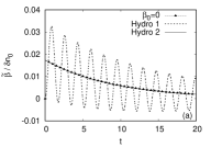
Refer to caption Refer to caption Refer to caption
Figure 9: Comparison between the numerical results (dotted lines and points) for ฮฒ~~๐›ฝ\widetilde{\beta} (first column), ฮดโ€‹P~~๐›ฟ๐‘ƒ\widetilde{\delta P} (second column) and ฮ ~~ฮ \widetilde{\Pi} (third column) and the corresponding analytic predictions of the first-order (dotted lines) and second-order (continuous lines) hydrodynamics when ฯ„ฮ =ฯ„subscript๐œฮ ๐œ\tau_{\Pi}=\tau and the Chapman-Enskog value (26b) for ฮป๐œ†\lambda is employed. The initial conditions for the plots on the first line correspond to Case 2b, i.e. ฮฒ0=ฮดโ€‹P0=0subscript๐›ฝ0๐›ฟsubscript๐‘ƒ00\beta_{0}=\delta P_{0}=0 and ฮดโ€‹n0=10โˆ’3๐›ฟsubscript๐‘›0superscript103\delta n_{0}=10^{-3}. On the second line, ฮฒ0subscript๐›ฝ0\beta_{0} is increased to 10โˆ’5superscript10510^{-5} and on the third line, ฮฒ0=10โˆ’3subscript๐›ฝ0superscript103\beta_{0}=10^{-3}. All curves are normalised with respect to ฮดโ€‹n0=10โˆ’3๐›ฟsubscript๐‘›0superscript103\delta n_{0}=10^{-3} and ฯ„=0.0083๐œ0.0083\tau=0.0083 was used throughout the simulations.

The non-adiabatic case can be analysed when the system is initialized according to Case 2b, when ฮฒ0=ฮดโ€‹P0=0subscript๐›ฝ0๐›ฟsubscript๐‘ƒ00\beta_{0}=\delta P_{0}=0. This case is particularly simple since, according to Eq.ย (77b), ฮฒฮท,โˆ—=0subscript๐›ฝ๐œ‚0\beta_{\eta,*}=0 for all ฮทโˆˆ{r,c,s}๐œ‚๐‘Ÿ๐‘๐‘ \eta\in\{r,c,s\}. The only non-vanishing integration constants are ฮฒฮป,ssubscript๐›ฝ๐œ†๐‘ \beta_{\lambda,s} (overdamped case) and ฮฒยฏฮป,ssubscriptยฏ๐›ฝ๐œ†๐‘ \overline{\beta}_{\lambda,s} (underdamped case), which can be found from Eq.ย (77a):

(ฮฒฮป,sฮฒยฏฮป,s)=((ฮฑฮป,d2โˆ’ฮฑฮป,o2)/ฮฑฮป,o(ฮฑยฏฮป,d2+ฮฑยฏฮป,o2)/ฮฑยฏฮป,o)โ€‹ฮดโ€‹n0kโ€‹n0.matrixsubscript๐›ฝ๐œ†๐‘ subscriptยฏ๐›ฝ๐œ†๐‘ matrixsuperscriptsubscript๐›ผ๐œ†๐‘‘2superscriptsubscript๐›ผ๐œ†๐‘œ2subscript๐›ผ๐œ†๐‘œsuperscriptsubscriptยฏ๐›ผ๐œ†๐‘‘2superscriptsubscriptยฏ๐›ผ๐œ†๐‘œ2subscriptยฏ๐›ผ๐œ†๐‘œ๐›ฟsubscript๐‘›0๐‘˜subscript๐‘›0\begin{pmatrix}\beta_{\lambda,s}\\ \overline{\beta}_{\lambda,s}\end{pmatrix}=\begin{pmatrix}(\alpha_{\lambda,d}^{2}-\alpha_{\lambda,o}^{2})/\alpha_{\lambda,o}\\ (\overline{\alpha}_{\lambda,d}^{2}+\overline{\alpha}_{\lambda,o}^{2})/\overline{\alpha}_{\lambda,o}\end{pmatrix}\frac{\delta n_{0}}{kn_{0}}. (80)

Noting that ฮดโ€‹P~=ฮ ~=0~๐›ฟ๐‘ƒ~ฮ 0\widetilde{\delta P}=\widetilde{\Pi}=0 by virtue of Eq.ย (73), the full solution in the overdamped case reads:

ฮฒ~=~๐›ฝabsent\displaystyle\widetilde{\beta}= ฮดโ€‹n0kโ€‹n0โ€‹ฮฑฮป,d2โˆ’ฮฑฮป,o2ฮฑฮป,oโ€‹eโˆ’ฮฑฮป,dโ€‹tโ€‹sinhโกฮฑฮป,oโ€‹t,๐›ฟsubscript๐‘›0๐‘˜subscript๐‘›0superscriptsubscript๐›ผ๐œ†๐‘‘2superscriptsubscript๐›ผ๐œ†๐‘œ2subscript๐›ผ๐œ†๐‘œsuperscript๐‘’subscript๐›ผ๐œ†๐‘‘๐‘กsubscript๐›ผ๐œ†๐‘œ๐‘ก\displaystyle\frac{\delta n_{0}}{kn_{0}}\frac{\alpha_{\lambda,d}^{2}-\alpha_{\lambda,o}^{2}}{\alpha_{\lambda,o}}e^{-\alpha_{\lambda,d}t}\sinh\alpha_{\lambda,o}t,
ฮดโ€‹n~=~๐›ฟ๐‘›absent\displaystyle\widetilde{\delta n}= ฮดโ€‹n0โ€‹(coshโกฮฑฮป,oโ€‹t+ฮฑฮป,dฮฑฮป,oโ€‹sinhโกฮฑฮป,oโ€‹t)โ€‹eโˆ’ฮฑฮป,dโ€‹t,๐›ฟsubscript๐‘›0subscript๐›ผ๐œ†๐‘œ๐‘กsubscript๐›ผ๐œ†๐‘‘subscript๐›ผ๐œ†๐‘œsubscript๐›ผ๐œ†๐‘œ๐‘กsuperscript๐‘’subscript๐›ผ๐œ†๐‘‘๐‘ก\displaystyle\delta n_{0}\left(\cosh\alpha_{\lambda,o}t+\frac{\alpha_{\lambda,d}}{\alpha_{\lambda,o}}\sinh\alpha_{\lambda,o}t\right)e^{-\alpha_{\lambda,d}t},
q~=~๐‘žabsent\displaystyle\widetilde{q}= โˆ’4โ€‹P0โ€‹ฮดโ€‹n0kโ€‹n0โ€‹ฮฑฮป,d2โˆ’ฮฑฮป,o2ฮฑฮป,oโ€‹eโˆ’ฮฑฮป,dโ€‹tโ€‹sinhโกฮฑฮป,oโ€‹t,4subscript๐‘ƒ0๐›ฟsubscript๐‘›0๐‘˜subscript๐‘›0superscriptsubscript๐›ผ๐œ†๐‘‘2superscriptsubscript๐›ผ๐œ†๐‘œ2subscript๐›ผ๐œ†๐‘œsuperscript๐‘’subscript๐›ผ๐œ†๐‘‘๐‘กsubscript๐›ผ๐œ†๐‘œ๐‘ก\displaystyle-4P_{0}\frac{\delta n_{0}}{kn_{0}}\frac{\alpha_{\lambda,d}^{2}-\alpha_{\lambda,o}^{2}}{\alpha_{\lambda,o}}e^{-\alpha_{\lambda,d}t}\sinh\alpha_{\lambda,o}t, (81a)
while in the underdamped case, the solution reads:
ฮฒ~=~๐›ฝabsent\displaystyle\widetilde{\beta}= ฮดโ€‹n0kโ€‹n0โ€‹ฮฑยฏฮป,d2+ฮฑยฏฮป,o2ฮฑยฏฮป,oโ€‹eโˆ’ฮฑยฏฮป,dโ€‹tโ€‹sinโกฮฑยฏฮป,oโ€‹t,๐›ฟsubscript๐‘›0๐‘˜subscript๐‘›0superscriptsubscriptยฏ๐›ผ๐œ†๐‘‘2superscriptsubscriptยฏ๐›ผ๐œ†๐‘œ2subscriptยฏ๐›ผ๐œ†๐‘œsuperscript๐‘’subscriptยฏ๐›ผ๐œ†๐‘‘๐‘กsubscriptยฏ๐›ผ๐œ†๐‘œ๐‘ก\displaystyle\frac{\delta n_{0}}{kn_{0}}\frac{\overline{\alpha}_{\lambda,d}^{2}+\overline{\alpha}_{\lambda,o}^{2}}{\overline{\alpha}_{\lambda,o}}e^{-\overline{\alpha}_{\lambda,d}t}\sin\overline{\alpha}_{\lambda,o}t,
ฮดโ€‹n~=~๐›ฟ๐‘›absent\displaystyle\widetilde{\delta n}= ฮดโ€‹n0โ€‹(cosโกฮฑยฏฮป,oโ€‹t+ฮฑยฏฮป,dฮฑยฏฮป,oโ€‹sinโกฮฑยฏฮป,oโ€‹t)โ€‹eโˆ’ฮฑยฏฮป,dโ€‹t,๐›ฟsubscript๐‘›0subscriptยฏ๐›ผ๐œ†๐‘œ๐‘กsubscriptยฏ๐›ผ๐œ†๐‘‘subscriptยฏ๐›ผ๐œ†๐‘œsubscriptยฏ๐›ผ๐œ†๐‘œ๐‘กsuperscript๐‘’subscriptยฏ๐›ผ๐œ†๐‘‘๐‘ก\displaystyle\delta n_{0}\left(\cos\overline{\alpha}_{\lambda,o}t+\frac{\overline{\alpha}_{\lambda,d}}{\overline{\alpha}_{\lambda,o}}\sin\overline{\alpha}_{\lambda,o}t\right)e^{-\overline{\alpha}_{\lambda,d}t},
q~=~๐‘žabsent\displaystyle\widetilde{q}= โˆ’4โ€‹P0โ€‹ฮดโ€‹n0kโ€‹n0โ€‹ฮฑยฏฮป,d2+ฮฑยฏฮป,o2ฮฑยฏฮป,oโ€‹eโˆ’ฮฑยฏฮป,dโ€‹tโ€‹sinโกฮฑยฏฮป,oโ€‹t.4subscript๐‘ƒ0๐›ฟsubscript๐‘›0๐‘˜subscript๐‘›0superscriptsubscriptยฏ๐›ผ๐œ†๐‘‘2superscriptsubscriptยฏ๐›ผ๐œ†๐‘œ2subscriptยฏ๐›ผ๐œ†๐‘œsuperscript๐‘’subscriptยฏ๐›ผ๐œ†๐‘‘๐‘กsubscriptยฏ๐›ผ๐œ†๐‘œ๐‘ก\displaystyle-4P_{0}\frac{\delta n_{0}}{kn_{0}}\frac{\overline{\alpha}_{\lambda,d}^{2}+\overline{\alpha}_{\lambda,o}^{2}}{\overline{\alpha}_{\lambda,o}}e^{-\overline{\alpha}_{\lambda,d}t}\sin\overline{\alpha}_{\lambda,o}t. (81b)

In the first-order theory, Eqs.ย (40) and (38) predict that, when ฮฒ0=ฮดโ€‹P0=0subscript๐›ฝ0๐›ฟsubscript๐‘ƒ00\beta_{0}=\delta P_{0}=0, ฮฒcsubscript๐›ฝ๐‘\beta_{c} and ฮฒssubscript๐›ฝ๐‘ \beta_{s} become proportional to ฮดโ€‹n0๐›ฟsubscript๐‘›0\delta n_{0}, which also implies that ฮ ~~ฮ \widetilde{\Pi} and ฮดโ€‹P~~๐›ฟ๐‘ƒ\widetilde{\delta P} are non-zero. This prediction is in contradiction with the second-order theory results. This discrepancy holds for any value of ฯ„๐œ\tau, hence it cannot be considered a โ€œhigher orderโ€ (rarefaction) effect. Instead, it represents a fundamental flaw of the first-order theory, which can be explained as follows.

The solution ฮ ~=ฮดโ€‹P~=0~ฮ ~๐›ฟ๐‘ƒ0\widetilde{\Pi}=\widetilde{\delta P}=0 is supported in the first-order theory only by the ฮฑฮปsubscript๐›ผ๐œ†\alpha_{\lambda} mode, as indicated in Eq.ย (32). However, according to Eq.ย (32), ฮดโ€‹nฮป๐›ฟsubscript๐‘›๐œ†\delta n_{\lambda} is proportional to ฮฒฮปsubscript๐›ฝ๐œ†\beta_{\lambda}, such that requiring that ฮฒฮป=0subscript๐›ฝ๐œ†0\beta_{\lambda}=0 automatically implies ฮดโ€‹nฮป=0๐›ฟsubscript๐‘›๐œ†0\delta n_{\lambda}=0. Thus, the initial conditions corresponding to Case 2b cannot be imposed using only the ฮฑฮปsubscript๐›ผ๐œ†\alpha_{\lambda} mode, such that the ฮฑยฑsubscript๐›ผplus-or-minus\alpha_{\pm} modes also become excited. The existence of two modes ฮฑฮป,ยฑsubscript๐›ผ๐œ†plus-or-minus\alpha_{\lambda,\pm} in the second-order theory which support ฮ ~=ฮดโ€‹P~=0~ฮ ~๐›ฟ๐‘ƒ0\widetilde{\Pi}=\widetilde{\delta P}=0 (59) is sufficient to allow the initial conditions of Case 2b to be imposed without exciting the ฮฑฮท,โˆ—subscript๐›ผ๐œ‚\alpha_{\eta,*} modes, such that ฮ ~=P~=0~ฮ ~๐‘ƒ0\widetilde{\Pi}=\widetilde{P}=0 throughout the evolution.

The case discussed above is represented in the plots on the first line of Fig.ย 9, where the time evolution of ฮฒ~~๐›ฝ\widetilde{\beta}, ฮดโ€‹P~~๐›ฟ๐‘ƒ\widetilde{\delta P} and ฮ ~~ฮ \widetilde{\Pi} (normalised with respect to ฮดโ€‹n0๐›ฟsubscript๐‘›0\delta n_{0}) is represented for the initial conditions ฮดโ€‹n0=10โˆ’3๐›ฟsubscript๐‘›0superscript103\delta n_{0}=10^{-3}, ฮดโ€‹P0=0๐›ฟsubscript๐‘ƒ00\delta P_{0}=0 and ฮฒ0=0subscript๐›ฝ00\beta_{0}=0. Both the second-order theory and the numerical results indicate that ฮดโ€‹P~~๐›ฟ๐‘ƒ\widetilde{\delta P} and ฮ ~~ฮ \widetilde{\Pi} remain zero throughout the evolution, while the first-order result predicts oscillations of these quantities. Moreover, in the first-order theory, ฮฒ~~๐›ฝ\widetilde{\beta} presents strong oscillations about a decaying exponential, which are not present when the second-order theory is employed. It is worth mentioning that the evolution predicted by the second-order theory and captured by the numerical method is consistent with the evolution equations (17), which reduce for ฮดโ€‹P=ฮ =0๐›ฟ๐‘ƒฮ 0\delta P=\Pi=0 to:

q=โˆ’4โ€‹P0โ€‹ฮฒ,โˆ‚tฮดโ€‹n+n0โ€‹โˆ‚zฮฒ=0.formulae-sequence๐‘ž4subscript๐‘ƒ0๐›ฝsubscript๐‘ก๐›ฟ๐‘›subscript๐‘›0subscript๐‘ง๐›ฝ0q=-4P_{0}\beta,\qquad\partial_{t}\delta n+n_{0}\partial_{z}\beta=0. (82)

The above relations are also recovered for the ฮฑฮปsubscript๐›ผ๐œ†\alpha_{\lambda} mode (32) of the first order theory. However, the initial conditions ฮฒ0=ฮดโ€‹P0/P0=0subscript๐›ฝ0๐›ฟsubscript๐‘ƒ0subscript๐‘ƒ00\beta_{0}=\delta P_{0}/P_{0}=0 and ฮดโ€‹n0=10โˆ’3๐›ฟsubscript๐‘›0superscript103\delta n_{0}=10^{-3} cannot be imposed using only the ฮฑฮปsubscript๐›ผ๐œ†\alpha_{\lambda} mode, since according to Eq.ย (32), ฮดโ€‹nฮป=kโ€‹n0โ€‹ฮฒฮป/ฮฑฮป๐›ฟsubscript๐‘›๐œ†๐‘˜subscript๐‘›0subscript๐›ฝ๐œ†subscript๐›ผ๐œ†\delta n_{\lambda}=kn_{0}\beta_{\lambda}/\alpha_{\lambda} implies that ฮดโ€‹n0๐›ฟsubscript๐‘›0\delta n_{0} is proportional to ฮฒฮปsubscript๐›ฝ๐œ†\beta_{\lambda}. Thus, setting ฮฒ0=0subscript๐›ฝ00\beta_{0}=0 and ฮดโ€‹n0โ‰ 0๐›ฟsubscript๐‘›00\delta n_{0}\neq 0 automatically excites the modes ฮดโ€‹nยฑ๐›ฟsubscript๐‘›plus-or-minus\delta n_{\pm} and ฮฒยฑsubscript๐›ฝplus-or-minus\beta_{\pm}, which no longer satisfy Eq.ย (82), such that the solution becomes contaminated with the addition of oscillatory modes.

The discussion in the preceding paragraph suggests that the first-order theory cannot fully recover the hydrodynamic regime (small ฯ„๐œ\tau) of the decaying longitudinal wave when the initialisation is performed according to Case 2b, i.e. ฮฒ0=ฮดโ€‹P0=0subscript๐›ฝ0๐›ฟsubscript๐‘ƒ00\beta_{0}=\delta P_{0}=0 and ฮดโ€‹n0=10โˆ’3๐›ฟsubscript๐‘›0superscript103\delta n_{0}=10^{-3}. It is instructive to further test if this conclusion holds at non-vanishing values of ฮฒ0subscript๐›ฝ0\beta_{0}, while keeping ฮดโ€‹P0=0๐›ฟsubscript๐‘ƒ00\delta P_{0}=0. The second and third lines of Fig.ย 9 show the evolution of ฮฒ~~๐›ฝ\widetilde{\beta}, ฮดโ€‹P~~๐›ฟ๐‘ƒ\widetilde{\delta P} and ฮ ~~ฮ \widetilde{\Pi} (again normalised with respect to ฮดโ€‹n0๐›ฟsubscript๐‘›0\delta n_{0}) when ฮฒ0=10โˆ’5subscript๐›ฝ0superscript105\beta_{0}=10^{-5} and ฮฒ0=10โˆ’3subscript๐›ฝ0superscript103\beta_{0}=10^{-3}, respectively. At ฮฒ0=10โˆ’5subscript๐›ฝ0superscript105\beta_{0}=10^{-5}, the first-order theory predicts oscillations which are (nearly) in antiphase to the numerical and second-order theory results. When ฮฒ0=10โˆ’3subscript๐›ฝ0superscript103\beta_{0}=10^{-3}, the discrepancy between the curves corresponding to the first-order theory and the numerical and second-order theory results is no longer visible.

Refer to caption
Refer to caption
Figure 10: (a) Numerical results (dotted lines and points) for the evolution of q~/ฯ„โ€‹ฮดโ€‹n0~๐‘ž๐œ๐›ฟsubscript๐‘›0\widetilde{q}/\tau\delta n_{0} at various values of ฯ„๐œ\tau for ฮดโ€‹n0=10โˆ’3๐›ฟsubscript๐‘›0superscript103\delta n_{0}=10^{-3} (to ease the comparison, the horizontal axis shows t/ฯ„๐‘ก๐œt/\tau). The analytic curves corresponding to the first (43) and second (79) order hydrodynamics are shown using dotted and continuous lines, respectively. (b) Time evolution of q~/ฯ„โ€‹ฮดโ€‹n0~๐‘ž๐œ๐›ฟsubscript๐‘›0\widetilde{q}/\tau\delta n_{0} at ฯ„=0.1๐œ0.1\tau=0.1 and ฮดโ€‹n0=10โˆ’3๐›ฟsubscript๐‘›0superscript103\delta n_{0}=10^{-3}. The fitted curve corresponding to the first-order hydrodynamics is obtained by performing a nonlinear fit of Eq.ย (44) using ฮฑฮทsubscript๐›ผ๐œ‚\alpha_{\eta} and ฮฑosubscript๐›ผ๐‘œ\alpha_{o} as free parameters. In the second-order case, the nonlinear fit is performed on Eqs.ย (81a) and (81b) for the overdamped and underdamped cases by considering ฮฑฮป,dsubscript๐›ผ๐œ†๐‘‘\alpha_{\lambda,d} and ฮฑฮป,osubscript๐›ผ๐œ†๐‘œ\alpha_{\lambda,o} (ฮฑยฏฮป,dsubscriptยฏ๐›ผ๐œ†๐‘‘\overline{\alpha}_{\lambda,d} and ฮฑยฏฮป,osubscriptยฏ๐›ผ๐œ†๐‘œ\overline{\alpha}_{\lambda,o}) as free parameters. All non-fitted anayltic curves are obtained using the Chapman-Enskog value for ฮป0subscript๐œ†0\lambda_{0} (26b) and ฯ„q,0=1subscript๐œ๐‘ž01\tau_{q,0}=1 (49).

The ability of the second-order hydrodynamics to capture the relaxation of q~~๐‘ž\widetilde{q} from 00 at initial time to the value predicted by the first-order theory is investigated in Fig.ย 10(a). It can be seen that at small ฯ„๐œ\tau, q~~๐‘ž\widetilde{q} relaxes to the value predicted through the first-order theory with ฮป๐œ†\lambda given by the Chapman-Enskog expansion (26b) after a time tโˆผ5โ€‹ฯ„similar-to๐‘ก5๐œt\sim 5\tau. At ฯ„โ‰ณ0.1greater-than-or-equivalent-to๐œ0.1\tau\gtrsim 0.1, the first-order approximation seems to no longer agree with the numerical solution (as indicated in Sec.ย III.6), while the second-order approximation slowly loses its validity. In Fig.ย 10(b), the numerical result for the evolution of q~~๐‘ž\widetilde{q} at ฯ„=0.1๐œ0.1\tau=0.1 is compared to the first (44) and second (81a) order hydrodynamics predictions, specialised to the Chapman-Enskog case, when ฮป0=4/3subscript๐œ†043\lambda_{0}=4/3 and ฯ„q,0=1subscript๐œ๐‘ž01\tau_{q,0}=1. It can be seen that there is significant discrepancy between the analytic and numerical results. The curve labelled Hydro 1 (fit) represents the best fit of the functional form of the analytic solution (44) to the numerical results, with ฮฑฮปsubscript๐›ผ๐œ†\alpha_{\lambda} considered as a free parameter. The second-order fits are performed on the two functional forms (81a) and (81b), corresponding to the overdamped and underdamped cases, respectively. In the overdamped case, Eq.ย (81a) is fitted to the numerical data by considering ฮฑฮป,dsubscript๐›ผ๐œ†๐‘‘\alpha_{\lambda,d} and ฮฑฮป,osubscript๐›ผ๐œ†๐‘œ\alpha_{\lambda,o} as free parameters. In the underdamped case, ฮฑยฏฮป,dsubscriptยฏ๐›ผ๐œ†๐‘‘\overline{\alpha}_{\lambda,d} and ฮฑยฏฮป,osubscriptยฏ๐›ผ๐œ†๐‘œ\overline{\alpha}_{\lambda,o} are found by performing a nonlinear fit of Eq.ย (81b) with respect to the numerical data. It can be seen in Fig.ย 10(b) that, at ฯ„=0.1๐œ0.1\tau=0.1, the first- and underdamped second-order fits still present significant deviations from the numerical curve. However, the second-order overdamped fit is in very good agreement with the numerical result, validating the functional form (81a) for ฯ„โ‰ฒ0.1less-than-or-similar-to๐œ0.1\tau\lesssim 0.1.

Refer to caption
Refer to caption
Figure 11: Analysis with respect to ฯ„๐œ\tau of (a) ฮฑฮป,dsubscript๐›ผ๐œ†๐‘‘\alpha_{\lambda,d} and (b) ฮฑฮป,osubscript๐›ผ๐œ†๐‘œ\alpha_{\lambda,o} for the initial conditions of Case 2b (i.e. ฮฒ0=ฮดโ€‹P0=0subscript๐›ฝ0๐›ฟsubscript๐‘ƒ00\beta_{0}=\delta P_{0}=0 and ฮดโ€‹n0=10โˆ’3๐›ฟsubscript๐‘›0superscript103\delta n_{0}=10^{-3}). The analytic curve in (a) is ฮฑฮป,d=1/2โ€‹ฯ„subscript๐›ผ๐œ†๐‘‘12๐œ\alpha_{\lambda,d}=1/2\tau, while in (b), the analytic result (61) is represented using the Chapman-Enskog (continuous line) and Grad (dashed line) values for ฮป๐œ†\lambda, while ฯ„qsubscript๐œ๐‘ž\tau_{q} was taken equal to ฯ„๐œ\tau. The numerical curves shown with dotted lines and filled symbols are obtained by performing a nonlinear fit on the overdamped (OD) solution (81a) while considering ฮฑฮป,dsubscript๐›ผ๐œ†๐‘‘\alpha_{\lambda,d} and ฮฑฮป,osubscript๐›ผ๐œ†๐‘œ\alpha_{\lambda,o} as free parameters. The dotted lines with hollow symbols are obtained by fitting the values of ฮฑยฏฮป,dsubscriptยฏ๐›ผ๐œ†๐‘‘\overline{\alpha}_{\lambda,d} and ฮฑยฏฮป,osubscriptยฏ๐›ผ๐œ†๐‘œ\overline{\alpha}_{\lambda,o} to the numerical results using the underdamped solution (81b). The numerical curves represented with dashed lines and without points are obtained by piecing together the UD and OD results. The transition from the OD to the UD regime occurs when ฮฑฮป,o=0subscript๐›ผ๐œ†๐‘œ0\alpha_{\lambda,o}=0, as indicated by the spikes in (b).

Next, Fig.ย 11 shows an analysis of (ฮฑฮป,d,ฮฑฮป,o)subscript๐›ผ๐œ†๐‘‘subscript๐›ผ๐œ†๐‘œ(\alpha_{\lambda,d},\alpha_{\lambda,o}) and (ฮฑยฏฮป,d,ฮฑยฏฮป,o)subscriptยฏ๐›ผ๐œ†๐‘‘subscriptยฏ๐›ผ๐œ†๐‘œ(\overline{\alpha}_{\lambda,d},\overline{\alpha}_{\lambda,o}) as obtained by performing a two-parameter nonlinear fit of Eqs.ย (81a) and (81b) for the overdamped (OD) and underdamped (UD) regimes, respectively, to the numerical results obtained for ฮฒ~~๐›ฝ\widetilde{\beta}, ฮดโ€‹n~~๐›ฟ๐‘›\widetilde{\delta n} and q~~๐‘ž\widetilde{q}. Only the initialisation corresponding to Case 2b (i.e. ฮฒ0=ฮดโ€‹P0=0subscript๐›ฝ0๐›ฟsubscript๐‘ƒ00\beta_{0}=\delta P_{0}=0 and ฮดโ€‹n0=10โˆ’3๐›ฟsubscript๐‘›0superscript103\delta n_{0}=10^{-3}) is considered here. The numerical fit confirms that at small values of ฯ„๐œ\tau, ฮฑฮป,dsubscript๐›ผ๐œ†๐‘‘\alpha_{\lambda,d} and ฮฑฮป,oโ‰ƒ1/2โ€‹ฯ„similar-to-or-equalssubscript๐›ผ๐œ†๐‘œ12๐œ\alpha_{\lambda,o}\simeq 1/2\tau. Furthermore, the results shown in Fig.ย 11(a) for ฮฑฮปsubscript๐›ผ๐œ†\alpha_{\lambda} indicate that the UD regime is not valid when ฯ„โ‰ฒ0.2less-than-or-similar-to๐œ0.2\tau\lesssim 0.2, while the OD regime loses applicability when ฯ„โ‰ณ0.1greater-than-or-equivalent-to๐œ0.1\tau\gtrsim 0.1. This can also be seen in Fig.ย 11(b), where the strong spikes indicate the points where ฮฑฮป,o=0subscript๐›ผ๐œ†๐‘œ0\alpha_{\lambda,o}=0, i.e. where the transition from the UD to the OD regime occurs. According to Eq.ย (60), this happens when ฯ„=ฯ„ฮป,limCEโ‰ƒ0.138๐œsuperscriptsubscript๐œ๐œ†limCEsimilar-to-or-equals0.138\tau=\tau_{\lambda,{\rm lim}}^{\rm CE}\simeq 0.138 and ฯ„=ฯ„ฮป,limGโ‰ƒ0.1779๐œsuperscriptsubscript๐œ๐œ†limGsimilar-to-or-equals0.1779\tau=\tau_{\lambda,{\rm lim}}^{\rm G}\simeq 0.1779 when the Chapman-Enskog (26b) and Grad (26a) values for ฮป0subscript๐œ†0\lambda_{0} are used, respectively. The above numerical analysis indicates that ฯ„ฮป,limโ‰ƒ0.199similar-to-or-equalssubscript๐œ๐œ†lim0.199\tau_{\lambda,{\rm lim}}\simeq 0.199 (in the case of ฮดโ€‹n~~๐›ฟ๐‘›\widetilde{\delta n}) and ฯ„ฮป,limโ‰ƒ0.183similar-to-or-equalssubscript๐œ๐œ†lim0.183\tau_{\lambda,{\rm lim}}\simeq 0.183 (in the case of ฮฒ~~๐›ฝ\widetilde{\beta} and q~~๐‘ž\widetilde{q}), higher than both the Chapman-Enskog and the Grad predictions.

Refer to caption
Refer to caption
Figure 12: Analysis with respect to ฯ„๐œ\tau of (a) ฯ„qsubscript๐œ๐‘ž\tau_{q} and (b) ฮป๐œ†\lambda for the initial conditions of Case 2b (i.e. ฮฒ0=ฮดโ€‹P0=0subscript๐›ฝ0๐›ฟsubscript๐‘ƒ00\beta_{0}=\delta P_{0}=0 and ฮดโ€‹n0=10โˆ’3๐›ฟsubscript๐‘›0superscript103\delta n_{0}=10^{-3}). The analytic curve shown in (a) using a continuous line is ฯ„q=ฯ„subscript๐œ๐‘ž๐œ\tau_{q}=\tau, while in (b), the analytic curves correspond to the Chapman-Enskog (continuous line) and Grad (dotted line) values for ฮป๐œ†\lambda, given in Eqs.ย (26b) and (26a), respectively. The numerical results are obtained as explained in Sec.ย IV.5.

The analysis of the relaxation time ฯ„qsubscript๐œ๐‘ž\tau_{q} and the heat conductivity ฮป๐œ†\lambda is presented in Fig.ย 12. Starting from the numerical fits of ฮฑฮป,dsubscript๐›ผ๐œ†๐‘‘\alpha_{\lambda,d} and ฮฑฮป,osubscript๐›ผ๐œ†๐‘œ\alpha_{\lambda,o}, where the overdamped (OD) and underdamped (UD) values are taken when ฯ„<ฯ„ฮป,lim๐œsubscript๐œ๐œ†lim\tau<\tau_{\lambda,{\rm lim}} and ฯ„>ฯ„ฮป,lim๐œsubscript๐œ๐œ†lim\tau>\tau_{\lambda,{\rm lim}}, respectively, the values of ฮป๐œ†\lambda and ฯ„qsubscript๐œ๐‘ž\tau_{q} are found by requiring that the roots ฮฑฮป,ยฑsubscript๐›ผ๐œ†plus-or-minus\alpha_{\lambda,\pm} (58) satisfy:

ฮฑฮป,++ฮฑฮป,โˆ’2=ฮฑฮป,d,|ฮฑฮป,+โˆ’ฮฑฮป,โˆ’2|=ฮฑฮป,o,formulae-sequencesubscript๐›ผ๐œ†subscript๐›ผ๐œ†2subscript๐›ผ๐œ†๐‘‘subscript๐›ผ๐œ†subscript๐›ผ๐œ†2subscript๐›ผ๐œ†๐‘œ\frac{\alpha_{\lambda,+}+\alpha_{\lambda,-}}{2}=\alpha_{\lambda,d},\qquad\left|\frac{\alpha_{\lambda,+}-\alpha_{\lambda,-}}{2}\right|=\alpha_{\lambda,o}, (83)

where the absolute value is interpreted in the usual sense in the case when ฮฑฮป,ยฑsubscript๐›ผ๐œ†plus-or-minus\alpha_{\lambda,\pm} are complex numbers. The results for ฯ„qsubscript๐œ๐‘ž\tau_{q} and ฮป๐œ†\lambda are shown in Figs.ย 12(a) and 12(b), respectively. It can be seen that the numerical results for ฯ„qsubscript๐œ๐‘ž\tau_{q} agree with the theoretical prediction ฯ„q=ฯ„subscript๐œ๐‘ž๐œ\tau_{q}=\tau at small values of ฯ„๐œ\tau, while for larger values of ฯ„๐œ\tau, ฯ„qsubscript๐œ๐‘ž\tau_{q} seems to reach a plateau. The curve representing the numerical results for ฮป๐œ†\lambda is practically overlapped with the Chapman-Enskog prediction (26b), while at larger values of ฯ„๐œ\tau, ฮป๐œ†\lambda seems to reach a plateau, in good qualitative agreement with the predictions of the first-order theory presented in Fig.ย 5.

IV.6 Summary

In this section, a particular form of the second-order hydrodynamics equations was employed to study the attenuation of a longitudinal wave in the linearised regime. More precisely, the choice ฮฑ1=โˆ’1/4โ€‹P0subscript๐›ผ114subscript๐‘ƒ0\alpha_{1}=-1/4P_{0} was made for the coupling constant between the shear pressure ฮ ฮ \Pi and heat flux q๐‘žq in the theory presented in Refs.ย hiscock83 ; rezzolla13 , in order to ensure consistency with the first-order hydrodynamics analysis presented in Sec.ย III.

The main aim of this section was to confirm that the second-order hydrodynamics correctly describes the relaxation process of ฮ ฮ \Pi and q๐‘žq from essentially arbitrary initial values (both vanish at initial time in the analysis presented in this paper) to some non-zero value which agrees with the prediction of the first-order theory at small enough values of ฯ„๐œ\tau. This is shown in Figs.ย 6 and 10, while the values of the relaxation times ฯ„ฮ subscript๐œฮ \tau_{\Pi} and ฯ„qsubscript๐œ๐‘ž\tau_{q} are analysed with respect to the relaxation time ฯ„๐œ\tau of the Anderson-Witting model in Figs.ย 8 and 12.

During this analysis, a fundamental limitation of the first-order theory was pointed out, which can be summarised as follows. If at initial time, the velocity and pressure perturbations vanish (i.e. ฮฒ0=ฮดโ€‹P0=0subscript๐›ฝ0๐›ฟsubscript๐‘ƒ00\beta_{0}=\delta P_{0}=0), the pressure ฮดโ€‹P~~๐›ฟ๐‘ƒ\widetilde{\delta P} and shear stress ฮ ~~ฮ \widetilde{\Pi} perturbations remain zero at all later times, while the attenuation of ฮฒ~~๐›ฝ\widetilde{\beta} is purely evanescent (non-oscillatory). This result is obtained analytically in the second-order theory and is confirmed via numerical simulations in Fig.ย 9. On the other hand, the first-order theory predicts that ฮดโ€‹P~~๐›ฟ๐‘ƒ\widetilde{\delta P} and ฮ ~~ฮ \widetilde{\Pi} are proportional to ฮดโ€‹n0๐›ฟsubscript๐‘›0\delta n_{0} and ฮฒ~~๐›ฝ\widetilde{\beta} has an oscillatory component the amplitude of which is proportional to ฯ„๐œ\tau. This leads to the conclusion that the first-order theory cannot correctly describe this particular dissipative process, even when the relaxation time is small.

V Moment method

The analysis presented in the previous sections provides indication that the correct expresions for the transport coefficients ฮป๐œ†\lambda and ฮท๐œ‚\eta are obtained using the Chapman-Enskog procedure. Recently denicol12 , it was shown that one of the main drawbacks of the moment method as originally employed by Israel and Stewart israel79 is that the distribution function f๐‘“f is expanded with respect to the nonorthogonal basis formed of powers of the particle four-momentum pฮผsuperscript๐‘๐œ‡p^{\mu}. Truncating this series at a finite order discards an infinite number of terms of first-order with respect to the Knudsen number KnKn{\rm Kn} (in the Anderson-Witting model, Knโˆผฯ„similar-toKn๐œ{\rm Kn}\sim\tau). The solution proposed in Ref.ย denicol12 was to expand f๐‘“f in terms of irreducible tensors with respect to the particle momentum pฮผsuperscript๐‘๐œ‡p^{\mu}. The proposed scheme recovers the expressions for the transport coefficients ฮป๐œ†\lambda and ฮท๐œ‚\eta obtained using the Chapman-Enskog expansion.

In this section, a moment-based method similar to the one introduced in Ref.ย denicol12 is considered. Spherical coordinates {p,ฮธ,ฯ†}๐‘๐œƒ๐œ‘\{p,\theta,\varphi\} are employed in the momentum space and the distribution function f๐‘“f is expanded with respect to the generalised Laguerre polynomials for the momentum magnitude p๐‘p, the Legendre polynomials for ฮพ=cosโกฮธ๐œ‰๐œƒ\xi=\cos\theta and the trigonometric basis {cosโกmโ€‹ฯ†,sinโกmโ€‹ฯ†}๐‘š๐œ‘๐‘š๐œ‘\{\cos m\varphi,\sin m\varphi\} for ฯ†๐œ‘\varphi. Due to the symmetries of the system, f๐‘“f can be considered independent of ฯ†๐œ‘\varphi, such that only the p๐‘p and ฮพ๐œ‰\xi expansions will be discussed. Truncating the system at order NL=1subscript๐‘๐ฟ1N_{L}=1 and Nฮพ=2subscript๐‘๐œ‰2N_{\xi}=2 with respect to the Laguerre and Legendre polynomials, respectively, yields a system of six equations for the five hydrodynamic variables ฮดโ€‹n๐›ฟ๐‘›\delta n, ฮฒ๐›ฝ\beta, ฮดโ€‹P๐›ฟ๐‘ƒ\delta P, q๐‘žq and ฮ ฮ \Pi, as well as a non-hydrodynamic variable. The importance of this sixth variable in establishing the symmetry between the shear stress and heat flux solutions is illustrated, such that the underdamped (UD) and overdamped (OD) regimes discussed in Sec.ย IV are represented unitarily in this new solution.

V.1 Constitutive relations

In this section, the longitudinal wave problem is again approached, but this time by employing a moment method. Instead of performing the standard Grad-like expansion of f๐‘“f in terms of polynomials in pฮผsuperscript๐‘๐œ‡p^{\mu}, f๐‘“f is expanded following Refs.ย blaga17aip ; blaga17prc as follows:

f=12โ€‹ฯ€โ€‹T03โ€‹eโˆ’p/T0โ€‹โˆ‘โ„“=0โˆž1(โ„“+1)โ€‹(โ„“+2)โ€‹โ„ฑโ„“โ€‹Lโ„“(2)โ€‹(p/T0),๐‘“12๐œ‹superscriptsubscript๐‘‡03superscript๐‘’๐‘subscript๐‘‡0superscriptsubscriptโ„“01โ„“1โ„“2subscriptโ„ฑโ„“subscriptsuperscript๐ฟ2โ„“๐‘subscript๐‘‡0f=\frac{1}{2\pi T_{0}^{3}}e^{-p/T_{0}}\sum_{\ell=0}^{\infty}\frac{1}{(\ell+1)(\ell+2)}\mathcal{F}_{\ell}L^{(2)}_{\ell}(p/T_{0}), (84)

where Lโ„“(2)โ€‹(z)subscriptsuperscript๐ฟ2โ„“๐‘งL^{(2)}_{\ell}(z) are the generalised Laguerre polynomial of type 222 and order โ„“โ„“\ell, which satisfy the following orthogonality relation:

โˆซ0โˆž๐‘‘zโ€‹z2โ€‹eโˆ’zโ€‹Lโ„“(2)โ€‹(z)โ€‹Lโ„“โ€ฒ(2)โ€‹(z)=(โ„“+1)โ€‹(โ„“+2)โ€‹ฮดโ„“,โ„“โ€ฒ.superscriptsubscript0differential-d๐‘งsuperscript๐‘ง2superscript๐‘’๐‘งsubscriptsuperscript๐ฟ2โ„“๐‘งsubscriptsuperscript๐ฟ2superscriptโ„“โ€ฒ๐‘งโ„“1โ„“2subscript๐›ฟโ„“superscriptโ„“โ€ฒ\int_{0}^{\infty}dz\,z^{2}\,e^{-z}L^{(2)}_{\ell}(z)L^{(2)}_{\ell^{\prime}}(z)=(\ell+1)(\ell+2)\delta_{\ell,\ell^{\prime}}. (85)

Thus, the coefficients โ„ฑโ„“subscriptโ„ฑโ„“\mathcal{F}_{\ell} can be obtained as follows:

โ„ฑโ„“=2โ€‹ฯ€โ€‹โˆซ0โˆž๐‘‘pโ€‹p2โ€‹fโ€‹Lโ„“(2)โ€‹(p/T0).subscriptโ„ฑโ„“2๐œ‹superscriptsubscript0differential-d๐‘superscript๐‘2๐‘“superscriptsubscript๐ฟโ„“2๐‘subscript๐‘‡0\mathcal{F}_{\ell}=2\pi\int_{0}^{\infty}dp\,p^{2}\,f\,L_{\ell}^{(2)}(p/T_{0}). (86)

Multiplying the Boltzmann equation (18), valid only in the linearised regime of the longitudinal wave problem, by p2โ€‹Lโ„“(2)โ€‹(p/T0)superscript๐‘2superscriptsubscript๐ฟโ„“2๐‘subscript๐‘‡0p^{2}L_{\ell}^{(2)}(p/T_{0}) and integrating over p๐‘p yields:

โˆ‚tโ„ฑโ„“+ฮพโ€‹โˆ‚zโ„ฑโ„“=โˆ’1ฯ„โ€‹(โ„ฑโ„“โˆ’โ„ฑโ„“(eq)),subscript๐‘กsubscriptโ„ฑโ„“๐œ‰subscript๐‘งsubscriptโ„ฑโ„“1๐œsubscriptโ„ฑโ„“subscriptsuperscriptโ„ฑeqโ„“\partial_{t}\mathcal{F}_{\ell}+\xi\partial_{z}\mathcal{F}_{\ell}=-\frac{1}{\tau}(\mathcal{F}_{\ell}-\mathcal{F}^{({\rm eq})}_{\ell}), (87)

where the coefficients โ„ฑโ„“(eq)subscriptsuperscriptโ„ฑeqโ„“\mathcal{F}^{({\rm eq})}_{\ell} corresponding to the equilibrium distribution function f(eq)superscript๐‘“eqf^{(\mathrm{eq})} are defined by analogy to Eq.ย (86):

โ„ฑโ„“(eq)=2โ€‹ฯ€โ€‹โˆซ0โˆž๐‘‘pโ€‹p2โ€‹f(eq)โ€‹Lโ„“(2)โ€‹(p/T0).superscriptsubscriptโ„ฑโ„“eq2๐œ‹superscriptsubscript0differential-d๐‘superscript๐‘2superscript๐‘“eqsuperscriptsubscript๐ฟโ„“2๐‘subscript๐‘‡0\mathcal{F}_{\ell}^{({\rm eq})}=2\pi\int_{0}^{\infty}dp\,p^{2}\,f^{(\mathrm{eq})}\,L_{\ell}^{(2)}(p/T_{0}). (88)

In the absence of collisions [i.e.ย when neglecting the right hand side in Eq.ย (87)], each coefficient โ„ฑโ„“subscriptโ„ฑโ„“\mathcal{F}_{\ell} evolves independently. Since f(eq)superscript๐‘“eqf^{(\mathrm{eq})} is constructed only in terms of Nฮผsuperscript๐‘๐œ‡N^{\mu} and Tฮผโ€‹ฮฝsuperscript๐‘‡๐œ‡๐œˆT^{\mu\nu}, which can be written entirely in terms of โ„ฑโ„“subscriptโ„ฑโ„“\mathcal{F}_{\ell} with โ„“=0โ„“0\ell=0 and โ„“=1โ„“1\ell=1, the evolution of Nฮผsuperscript๐‘๐œ‡N^{\mu} and Tฮผโ€‹ฮฝsuperscript๐‘‡๐œ‡๐œˆT^{\mu\nu} is fully determined by considering Eq.ย (87) only for โ„“=0โ„“0\ell=0 and โ„“=1โ„“1\ell=1 and neglecting all higher โ„“โ„“\ell terms blaga17prc .

The coefficients โ„ฑโ„“subscriptโ„ฑโ„“\mathcal{F}_{\ell} are further expanded with respect to ฮพ๐œ‰\xi using the complete set of Legendre polynomials Psโ€‹(ฮพ)subscript๐‘ƒ๐‘ ๐œ‰P_{s}(\xi):

โ„ฑโ„“=โˆ‘s=0โˆž2โ€‹s+12โ€‹โ„ฑโ„“,sโ€‹Psโ€‹(ฮพ),subscriptโ„ฑโ„“superscriptsubscript๐‘ 02๐‘ 12subscriptโ„ฑโ„“๐‘ subscript๐‘ƒ๐‘ ๐œ‰\mathcal{F}_{\ell}=\sum_{s=0}^{\infty}\frac{2s+1}{2}\mathcal{F}_{\ell,s}P_{s}(\xi), (89)

where the coefficients โ„ฑโ„“,ssubscriptโ„ฑโ„“๐‘ \mathcal{F}_{\ell,s} depend only on z๐‘งz and t๐‘กt and are obtained using the orthogonality of the Legendre polynomials as follows:

โ„ฑโ„“,s=โˆซโˆ’11๐‘‘ฮพโ€‹โ„ฑโ„“โ€‹Psโ€‹(ฮพ).subscriptโ„ฑโ„“๐‘ superscriptsubscript11differential-d๐œ‰subscriptโ„ฑโ„“subscript๐‘ƒ๐‘ ๐œ‰\mathcal{F}_{\ell,s}=\int_{-1}^{1}d\xi\,\mathcal{F}_{\ell}P_{s}(\xi). (90)

The coefficients โ„ฑโ„“,s(eq)superscriptsubscriptโ„ฑโ„“๐‘ eq\mathcal{F}_{\ell,s}^{({\rm eq})} corresponding to f(eq)superscript๐‘“eqf^{(\mathrm{eq})} can be defined in a similar manner:

โ„ฑโ„“,s(eq)=โˆซโˆ’11๐‘‘ฮพโ€‹โ„ฑโ„“(eq)โ€‹Psโ€‹(ฮพ).superscriptsubscriptโ„ฑโ„“๐‘ eqsuperscriptsubscript11differential-d๐œ‰superscriptsubscriptโ„ฑโ„“eqsubscript๐‘ƒ๐‘ ๐œ‰\mathcal{F}_{\ell,s}^{({\rm eq})}=\int_{-1}^{1}d\xi\,\mathcal{F}_{\ell}^{({\rm eq})}P_{s}(\xi). (91)

The expansion coefficients โ„ฑโ„“,ssubscriptโ„ฑโ„“๐‘ \mathcal{F}_{\ell,s} can be linked to Nฮผsuperscript๐‘๐œ‡N^{\mu} and Tฮผโ€‹ฮฝsuperscript๐‘‡๐œ‡๐œˆT^{\mu\nu} as follows:

โ„ฑ0,0=Ntโ‰ƒn0+ฮดโ€‹n,โ„ฑ0,1=Nzโ‰ƒn0โ€‹ฮฒ,formulae-sequencesubscriptโ„ฑ00superscript๐‘๐‘กsimilar-to-or-equalssubscript๐‘›0๐›ฟ๐‘›subscriptโ„ฑ01superscript๐‘๐‘งsimilar-to-or-equalssubscript๐‘›0๐›ฝ\displaystyle\mathcal{F}_{0,0}=N^{t}\simeq n_{0}+\delta n,\qquad\mathcal{F}_{0,1}=N^{z}\simeq n_{0}\beta,
โ„ฑ1,0=3โ€‹Ntโˆ’1T0โ€‹Ttโ€‹tโ‰ƒ3โ€‹n0โ€‹(ฮดโ€‹nn0โˆ’ฮดโ€‹PP0),subscriptโ„ฑ103superscript๐‘๐‘ก1subscript๐‘‡0superscript๐‘‡๐‘ก๐‘กsimilar-to-or-equals3subscript๐‘›0๐›ฟ๐‘›subscript๐‘›0๐›ฟ๐‘ƒsubscript๐‘ƒ0\displaystyle\mathcal{F}_{1,0}=3N^{t}-\frac{1}{T_{0}}T^{tt}\simeq 3n_{0}\left(\frac{\delta n}{n_{0}}-\frac{\delta P}{P_{0}}\right),
โ„ฑ1,1=3โ€‹Nzโˆ’1T0โ€‹Ttโ€‹zโ‰ƒโˆ’n0โ€‹ฮฒโˆ’qT0,subscriptโ„ฑ113superscript๐‘๐‘ง1subscript๐‘‡0superscript๐‘‡๐‘ก๐‘งsimilar-to-or-equalssubscript๐‘›0๐›ฝ๐‘žsubscript๐‘‡0\displaystyle\mathcal{F}_{1,1}=3N^{z}-\frac{1}{T_{0}}T^{tz}\simeq-n_{0}\beta-\frac{q}{T_{0}},
3โ€‹โ„ฑ0,2โˆ’โ„ฑ1,2โ‰ƒ3โ€‹ฮ 2โ€‹T0.similar-to-or-equals3subscriptโ„ฑ02subscriptโ„ฑ123ฮ 2subscript๐‘‡0\displaystyle 3\mathcal{F}_{0,2}-\mathcal{F}_{1,2}\simeq\frac{3\Pi}{2T_{0}}. (92)

The coefficients โ„ฑ0,2subscriptโ„ฑ02\mathcal{F}_{0,2} and โ„ฑ1,2subscriptโ„ฑ12\mathcal{F}_{1,2} on their own have no correspondent with respect to Nฮผsuperscript๐‘๐œ‡N^{\mu} and Tฮผโ€‹ฮฝsuperscript๐‘‡๐œ‡๐œˆT^{\mu\nu}. The equilibrium coefficients โ„ฑโ„“,s(eq)superscriptsubscriptโ„ฑโ„“๐‘ eq\mathcal{F}_{\ell,s}^{({\rm eq})} (โ„“=0,1โ„“01\ell=0,1 and s=0,1,2๐‘ 012s=0,1,2) can be found from Eq.ย (19):

โ„ฑ0,0(eq)โ‰ƒn0+ฮดโ€‹n,โ„ฑ0,1(eq)โ‰ƒn0โ€‹ฮฒ+q4โ€‹T0,formulae-sequencesimilar-to-or-equalssuperscriptsubscriptโ„ฑ00eqsubscript๐‘›0๐›ฟ๐‘›similar-to-or-equalssuperscriptsubscriptโ„ฑ01eqsubscript๐‘›0๐›ฝ๐‘ž4subscript๐‘‡0\displaystyle\mathcal{F}_{0,0}^{({\rm eq})}\simeq n_{0}+\delta n,\qquad\mathcal{F}_{0,1}^{({\rm eq})}\simeq n_{0}\beta+\frac{q}{4T_{0}},
โ„ฑ1,0(eq)โ‰ƒ3โ€‹n0โ€‹(ฮดโ€‹nn0โˆ’ฮดโ€‹PP0),โ„ฑ1,1(eq)โ‰ƒโˆ’n0โ€‹ฮฒโˆ’q4โ€‹T0,formulae-sequencesimilar-to-or-equalssuperscriptsubscriptโ„ฑ10eq3subscript๐‘›0๐›ฟ๐‘›subscript๐‘›0๐›ฟ๐‘ƒsubscript๐‘ƒ0similar-to-or-equalssuperscriptsubscriptโ„ฑ11eqsubscript๐‘›0๐›ฝ๐‘ž4subscript๐‘‡0\displaystyle\mathcal{F}_{1,0}^{({\rm eq})}\simeq 3n_{0}\left(\frac{\delta n}{n_{0}}-\frac{\delta P}{P_{0}}\right),\qquad\mathcal{F}_{1,1}^{({\rm eq})}\simeq-n_{0}\beta-\frac{q}{4T_{0}}, (93)

while โ„ฑ0,2(eq)โ‰ƒ0similar-to-or-equalssuperscriptsubscriptโ„ฑ02eq0\mathcal{F}_{0,2}^{({\rm eq})}\simeq 0 and โ„ฑ1,2(eq)โ‰ƒ0similar-to-or-equalssuperscriptsubscriptโ„ฑ12eq0\mathcal{F}_{1,2}^{({\rm eq})}\simeq 0.

Using the recurrence relation:

ฮพโ€‹Psโ€‹(ฮพ)=s+12โ€‹s+1โ€‹Ps+1โ€‹(ฮพ)+s2โ€‹s+1โ€‹Psโˆ’1โ€‹(ฮพ),๐œ‰subscript๐‘ƒ๐‘ ๐œ‰๐‘ 12๐‘ 1subscript๐‘ƒ๐‘ 1๐œ‰๐‘ 2๐‘ 1subscript๐‘ƒ๐‘ 1๐œ‰\xi P_{s}(\xi)=\frac{s+1}{2s+1}P_{s+1}(\xi)+\frac{s}{2s+1}P_{s-1}(\xi), (94)

Eq.ย (87) can be projected on the space of the Legendre polynomials as follows:

โˆ‚tโ„ฑโ„“,s+โˆ‚z(s2โ€‹s+1โ€‹โ„ฑโ„“,sโˆ’1+s+12โ€‹s+1โ€‹โ„ฑโ„“,s+1)=โˆ’1ฯ„โ€‹(โ„ฑโ„“,sโˆ’โ„ฑโ„“,s(eq)).subscript๐‘กsubscriptโ„ฑโ„“๐‘ subscript๐‘ง๐‘ 2๐‘ 1subscriptโ„ฑโ„“๐‘ 1๐‘ 12๐‘ 1subscriptโ„ฑโ„“๐‘ 11๐œsubscriptโ„ฑโ„“๐‘ superscriptsubscriptโ„ฑโ„“๐‘ eq\partial_{t}\mathcal{F}_{\ell,s}+\partial_{z}\left(\frac{s}{2s+1}\mathcal{F}_{\ell,s-1}+\frac{s+1}{2s+1}\mathcal{F}_{\ell,s+1}\right)\\ =-\frac{1}{\tau}(\mathcal{F}_{\ell,s}-\mathcal{F}_{\ell,s}^{({\rm eq})}). (95)

The above procedure produces an infinite system of equations corresponding to various values of (โ„“,s)โ„“๐‘ (\ell,s), where knowledge of โ„ฑโ„“,s+1subscriptโ„ฑโ„“๐‘ 1\mathcal{F}_{\ell,s+1} is required in order to determine the evolution of โ„ฑโ„“,ssubscriptโ„ฑโ„“๐‘ \mathcal{F}_{\ell,s}. As also discussed in Ref.ย blaga17prc , the above system can be closed at an order Q๐‘„Q by imposing โ„ฑโ„“,Q=0subscriptโ„ฑโ„“๐‘„0\mathcal{F}_{\ell,Q}=0. This procedure is intimately related to the numerical method employed in this paper (described in detail in Ref.ย blaga17prc and also summarised in Appendixย B). In particular, Q๐‘„Q represents the quadrature order of the model and the resulting system of equations is guaranteed to be hyperbolic. Since only the study of Nฮผsuperscript๐‘๐œ‡N^{\mu} and Tฮผโ€‹ฮฝsuperscript๐‘‡๐œ‡๐œˆT^{\mu\nu} is of interest in this section, only the case Q=3๐‘„3Q=3 will be considered henceforth, such that โ„ฑ0,3=โ„ฑ1,3=0subscriptโ„ฑ03subscriptโ„ฑ130\mathcal{F}_{0,3}=\mathcal{F}_{1,3}=0. The resulting set of equations can be written as:

โˆ‚tโ„ฑ0,0+โˆ‚zโ„ฑ0,1=subscript๐‘กsubscriptโ„ฑ00subscript๐‘งsubscriptโ„ฑ01absent\displaystyle\partial_{t}\mathcal{F}_{0,0}+\partial_{z}\mathcal{F}_{0,1}= โˆ’1ฯ„โ€‹(โ„ฑ0,0โˆ’โ„ฑ0,0(eq)),1๐œsubscriptโ„ฑ00superscriptsubscriptโ„ฑ00eq\displaystyle-\frac{1}{\tau}(\mathcal{F}_{0,0}-\mathcal{F}_{0,0}^{({\rm eq})}), (96a)
โˆ‚tโ„ฑ0,1+13โ€‹โˆ‚z(โ„ฑ0,0+2โ€‹โ„ฑ0,2)=subscript๐‘กsubscriptโ„ฑ0113subscript๐‘งsubscriptโ„ฑ002subscriptโ„ฑ02absent\displaystyle\partial_{t}\mathcal{F}_{0,1}+\frac{1}{3}\partial_{z}\left(\mathcal{F}_{0,0}+2\mathcal{F}_{0,2}\right)= โˆ’1ฯ„โ€‹(โ„ฑ0,1โˆ’โ„ฑ0,1(eq)),1๐œsubscriptโ„ฑ01superscriptsubscriptโ„ฑ01eq\displaystyle-\frac{1}{\tau}(\mathcal{F}_{0,1}-\mathcal{F}_{0,1}^{({\rm eq})}), (96b)
โˆ‚tโ„ฑ0,2+25โ€‹โˆ‚zโ„ฑ0,1=subscript๐‘กsubscriptโ„ฑ0225subscript๐‘งsubscriptโ„ฑ01absent\displaystyle\partial_{t}\mathcal{F}_{0,2}+\frac{2}{5}\partial_{z}\mathcal{F}_{0,1}= โˆ’1ฯ„โ€‹โ„ฑ0,2,1๐œsubscriptโ„ฑ02\displaystyle-\frac{1}{\tau}\mathcal{F}_{0,2}, (96c)
โˆ‚tโ„ฑ1,0+โˆ‚zโ„ฑ1,1=subscript๐‘กsubscriptโ„ฑ10subscript๐‘งsubscriptโ„ฑ11absent\displaystyle\partial_{t}\mathcal{F}_{1,0}+\partial_{z}\mathcal{F}_{1,1}= โˆ’1ฯ„โ€‹(โ„ฑ1,0โˆ’โ„ฑ1,0(eq)),1๐œsubscriptโ„ฑ10superscriptsubscriptโ„ฑ10eq\displaystyle-\frac{1}{\tau}(\mathcal{F}_{1,0}-\mathcal{F}_{1,0}^{({\rm eq})}), (96d)
โˆ‚tโ„ฑ1,1+13โ€‹โˆ‚z(โ„ฑ1,0+2โ€‹โ„ฑ1,2)=subscript๐‘กsubscriptโ„ฑ1113subscript๐‘งsubscriptโ„ฑ102subscriptโ„ฑ12absent\displaystyle\partial_{t}\mathcal{F}_{1,1}+\frac{1}{3}\partial_{z}\left(\mathcal{F}_{1,0}+2\mathcal{F}_{1,2}\right)= โˆ’1ฯ„โ€‹(โ„ฑ1,1โˆ’โ„ฑ1,1(eq)),1๐œsubscriptโ„ฑ11superscriptsubscriptโ„ฑ11eq\displaystyle-\frac{1}{\tau}(\mathcal{F}_{1,1}-\mathcal{F}_{1,1}^{({\rm eq})}), (96e)
โˆ‚tโ„ฑ1,2+25โ€‹โˆ‚zโ„ฑ1,1=subscript๐‘กsubscriptโ„ฑ1225subscript๐‘งsubscriptโ„ฑ11absent\displaystyle\partial_{t}\mathcal{F}_{1,2}+\frac{2}{5}\partial_{z}\mathcal{F}_{1,1}= โˆ’1ฯ„โ€‹โ„ฑ1,2.1๐œsubscriptโ„ฑ12\displaystyle-\frac{1}{\tau}\mathcal{F}_{1,2}. (96f)

The above system is closed. Substituting Eqs.ย (92) and (93) into Eq.ย (96), the conservation equations (17) can be obtained, together with the following constitutive equations:

ฯ„โ€‹โˆ‚tq+q=โˆ’ฯ„โ€‹P03โ€‹โˆ‚z(3โ€‹ฮดโ€‹PP0โˆ’4โ€‹ฮดโ€‹nn0)๐œsubscript๐‘ก๐‘ž๐‘ž๐œsubscript๐‘ƒ03subscript๐‘ง3๐›ฟ๐‘ƒsubscript๐‘ƒ04๐›ฟ๐‘›subscript๐‘›0\displaystyle\tau\partial_{t}q+q=-\frac{\tau P_{0}}{3}\partial_{z}\left(\frac{3\delta P}{P_{0}}-\frac{4\delta n}{n_{0}}\right)
+2โ€‹P0โ€‹ฯ„3โ€‹n0โ€‹โˆ‚z(โ„ฑ0,2+โ„ฑ1,2),2subscript๐‘ƒ0๐œ3subscript๐‘›0subscript๐‘งsubscriptโ„ฑ02subscriptโ„ฑ12\displaystyle\phantom{aaaaaaaaaaaaaaaaa}+\frac{2P_{0}\tau}{3n_{0}}\partial_{z}(\mathcal{F}_{0,2}+\mathcal{F}_{1,2}), (97a)
ฯ„โ€‹โˆ‚tฮ +ฮ =โˆ’16โ€‹ฯ„โ€‹P015โ€‹โˆ‚z(ฮฒ+q4โ€‹P0),๐œsubscript๐‘กฮ ฮ 16๐œsubscript๐‘ƒ015subscript๐‘ง๐›ฝ๐‘ž4subscript๐‘ƒ0\displaystyle\tau\partial_{t}\Pi+\Pi=-\frac{16\tau P_{0}}{15}\partial_{z}\left(\beta+\frac{q}{4P_{0}}\right), (97b)
(ฯ„โ€‹โˆ‚t+1)โ€‹(โ„ฑ0,2+โ„ฑ1,2)=2โ€‹n0โ€‹ฯ„5โ€‹P0โ€‹โˆ‚zq.๐œsubscript๐‘ก1subscriptโ„ฑ02subscriptโ„ฑ122subscript๐‘›0๐œ5subscript๐‘ƒ0subscript๐‘ง๐‘ž\displaystyle(\tau\partial_{t}+1)(\mathcal{F}_{0,2}+\mathcal{F}_{1,2})=\frac{2n_{0}\tau}{5P_{0}}\partial_{z}q. (97c)

Comparing the above equations to the second-order hydrodynamics constitutive equations (47), it can be seen that the transport coefficients have the following expressions:

ฮป=43โ€‹ฯ„โ€‹n0,ฮท=45โ€‹ฯ„โ€‹P0,ฯ„q=ฯ„,ฯ„ฮ =ฯ„.formulae-sequence๐œ†43๐œsubscript๐‘›0formulae-sequence๐œ‚45๐œsubscript๐‘ƒ0formulae-sequencesubscript๐œ๐‘ž๐œsubscript๐œฮ ๐œ\lambda=\frac{4}{3}\tau n_{0},\qquad\eta=\frac{4}{5}\tau P_{0},\qquad\tau_{q}=\tau,\qquad\tau_{\Pi}=\tau. (98)

The above relations confirm the Chapman-Enskog prediction (26b) for ฮป๐œ†\lambda and ฮท๐œ‚\eta and agree with the second-order hydrodynamics values for ฯ„qsubscript๐œ๐‘ž\tau_{q} and ฯ„ฮ subscript๐œฮ \tau_{\Pi} given in Eq.ย (49). Furthermore, the constitutive equation (97a) contains an extra term compared to the second-order hydrodynamics version (47a). A simple power counting shows that this term is cubic in the relaxation time ฯ„๐œ\tau, hence it cannot be present in the second-order hydroynamics theory.

V.2 Longitudinal waves: modes

Considering now the propagation of a wave with wave number k๐‘˜k, the ansatz (20) can be applied to the new variables โ„ฑ0,2subscriptโ„ฑ02\mathcal{F}_{0,2} and โ„ฑ1,2subscriptโ„ฑ12\mathcal{F}_{1,2} as follows:

โ„ฑ0,2=โ„ฑ~0,2โ€‹cosโกkโ€‹z,โ„ฑ1,2=โ„ฑ~1,2โ€‹cosโกkโ€‹z.formulae-sequencesubscriptโ„ฑ02subscript~โ„ฑ02๐‘˜๐‘งsubscriptโ„ฑ12subscript~โ„ฑ12๐‘˜๐‘ง\mathcal{F}_{0,2}=\widetilde{\mathcal{F}}_{0,2}\cos kz,\qquad\mathcal{F}_{1,2}=\widetilde{\mathcal{F}}_{1,2}\cos kz. (99)

The mode decomposition (21) can be applied to โ„ฑ~0,2subscript~โ„ฑ02\widetilde{\mathcal{F}}_{0,2} and โ„ฑ~1,2subscript~โ„ฑ12\widetilde{\mathcal{F}}_{1,2} as follows:

(โ„ฑ~0,2โ„ฑ~1,2)=โˆ‘ฮฑ(โ„ฑ0,2;ฮฑโ„ฑ1,2;ฮฑ)โ€‹eโˆ’ฮฑโ€‹t.matrixsubscript~โ„ฑ02subscript~โ„ฑ12subscript๐›ผmatrixsubscriptโ„ฑ02๐›ผsubscriptโ„ฑ12๐›ผsuperscript๐‘’๐›ผ๐‘ก\begin{pmatrix}\widetilde{\mathcal{F}}_{0,2}\\ \widetilde{\mathcal{F}}_{1,2}\end{pmatrix}=\sum_{\alpha}\begin{pmatrix}\mathcal{F}_{0,2;\alpha}\\ \mathcal{F}_{1,2;\alpha}\end{pmatrix}e^{-\alpha t}. (100)

Substituting the above expansions into Eqs.ย (96c) and (96f) gives:

โ„ฑ0,2;ฮฑ=subscriptโ„ฑ02๐›ผabsent\displaystyle\mathcal{F}_{0,2;\alpha}= โˆ’2โ€‹n0โ€‹ฯ„โ€‹k5โ€‹(1โˆ’ฮฑโ€‹ฯ„)โ€‹ฮฒฮฑ,2subscript๐‘›0๐œ๐‘˜51๐›ผ๐œsubscript๐›ฝ๐›ผ\displaystyle-\frac{2n_{0}\tau k}{5(1-\alpha\tau)}\beta_{\alpha},
โ„ฑ1,2;ฮฑ=subscriptโ„ฑ12๐›ผabsent\displaystyle\mathcal{F}_{1,2;\alpha}= 2โ€‹n0โ€‹ฯ„โ€‹k5โ€‹(1โˆ’ฮฑโ€‹ฯ„)โ€‹(ฮฒฮฑ+qฮฑP0).2subscript๐‘›0๐œ๐‘˜51๐›ผ๐œsubscript๐›ฝ๐›ผsubscript๐‘ž๐›ผsubscript๐‘ƒ0\displaystyle\frac{2n_{0}\tau k}{5(1-\alpha\tau)}\left(\beta_{\alpha}+\frac{q_{\alpha}}{P_{0}}\right). (101)

The moment method introduced in this section bears many similarities with the second-order hydrodynamics method discussed in Sec.ย IV. In particular, since the constitutive equations (97b) and (47b) for ฮ ฮ \Pi are the same in the two theories, Eqs.ย (54), (55) and (56) remain unchanged. The latter equation again can be solved either by setting qฮฑ=โˆ’4โ€‹P0โ€‹ฮฒฮฑsubscript๐‘ž๐›ผ4subscript๐‘ƒ0subscript๐›ฝ๐›ผq_{\alpha}=-4P_{0}\beta_{\alpha} or by setting the square bracket to 00. In the latter case, the allowed values for ฮฑ๐›ผ\alpha, namely ฮฑฮท,rsubscript๐›ผ๐œ‚๐‘Ÿ\alpha_{\eta,r} and ฮฑฮท,ยฑsubscript๐›ผ๐œ‚plus-or-minus\alpha_{\eta,\pm} can be written as in Sec.ย IV.2, being given in Eq.ย (64). For completeness, these expressions are reproduced below, specialised to the values of ฮท๐œ‚\eta, ฮป๐œ†\lambda, ฯ„qsubscript๐œ๐‘ž\tau_{q} and ฯ„ฮ subscript๐œฮ \tau_{\Pi} given in Eq.ย (98):

ฮฑฮท,r=subscript๐›ผ๐œ‚๐‘Ÿabsent\displaystyle\alpha_{\eta,r}= 13โ€‹ฯ„โ€‹[1+1Rฮทโ€‹(1โˆ’9โ€‹k2โ€‹ฯ„25)+Rฮท]13๐œdelimited-[]11subscript๐‘…๐œ‚19superscript๐‘˜2superscript๐œ25subscript๐‘…๐œ‚\displaystyle\frac{1}{3\tau}\left[1+\frac{1}{R_{\eta}}\left(1-\frac{9k^{2}\tau^{2}}{5}\right)+R_{\eta}\right]
โ‰ƒsimilar-to-or-equals\displaystyle\simeq 1ฯ„โˆ’2โ€‹ฮฑd+Oโ€‹(ฯ„3),1๐œ2subscript๐›ผ๐‘‘๐‘‚superscript๐œ3\displaystyle\frac{1}{\tau}-2\alpha_{d}+O(\tau^{3}),
ฮฑฮท,d=subscript๐›ผ๐œ‚๐‘‘absent\displaystyle\alpha_{\eta,d}= 13โ€‹ฯ„โ€‹[1โˆ’12โ€‹Rฮทโ€‹(1โˆ’9โ€‹k2โ€‹ฯ„25)โˆ’Rฮท2]13๐œdelimited-[]112subscript๐‘…๐œ‚19superscript๐‘˜2superscript๐œ25subscript๐‘…๐œ‚2\displaystyle\frac{1}{3\tau}\left[1-\frac{1}{2R_{\eta}}\left(1-\frac{9k^{2}\tau^{2}}{5}\right)-\frac{R_{\eta}}{2}\right]
โ‰ƒsimilar-to-or-equals\displaystyle\simeq ฮฑd+Oโ€‹(ฯ„3),subscript๐›ผ๐‘‘๐‘‚superscript๐œ3\displaystyle\alpha_{d}+O(\tau^{3}),
ฮฑฮท,o=subscript๐›ผ๐œ‚๐‘œabsent\displaystyle\alpha_{\eta,o}= 36โ€‹ฯ„โ€‹[1Rฮทโ€‹(1โˆ’9โ€‹k2โ€‹ฯ„25)โˆ’Rฮท]36๐œdelimited-[]1subscript๐‘…๐œ‚19superscript๐‘˜2superscript๐œ25subscript๐‘…๐œ‚\displaystyle\frac{\sqrt{3}}{6\tau}\left[\frac{1}{R_{\eta}}\left(1-\frac{9k^{2}\tau^{2}}{5}\right)-R_{\eta}\right]
โ‰ƒsimilar-to-or-equals\displaystyle\simeq k3+Oโ€‹(ฯ„2),๐‘˜3๐‘‚superscript๐œ2\displaystyle\frac{k}{\sqrt{3}}+O(\tau^{2}), (102)

where ฮฑd=2โ€‹k2โ€‹ฯ„/15subscript๐›ผ๐‘‘2superscript๐‘˜2๐œ15\alpha_{d}=2k^{2}\tau/15 is the first-order coefficient given in Eq.ย (35) and Rฮทsubscript๐‘…๐œ‚R_{\eta} (65) becomes:

Rฮท={(1โˆ’3โ€‹kโ€‹ฯ„โ€‹Rฮท,aux+95โ€‹k2โ€‹ฯ„2)1/3,ฯ„<ฯ„ฮท,lim,โˆ’(โˆ’1+3โ€‹kโ€‹ฯ„โ€‹Rฮท,auxโˆ’95โ€‹k2โ€‹ฯ„2)1/3,ฯ„>ฯ„ฮท,lim.subscript๐‘…๐œ‚casessuperscript13๐‘˜๐œsubscript๐‘…๐œ‚aux95superscript๐‘˜2superscript๐œ213๐œsubscript๐œ๐œ‚limsuperscript13๐‘˜๐œsubscript๐‘…๐œ‚aux95superscript๐‘˜2superscript๐œ213๐œsubscript๐œ๐œ‚limR_{\eta}=\begin{cases}\left(1-3k\tau\sqrt{R_{\eta,{\rm aux}}}+\frac{9}{5}k^{2}\tau^{2}\right)^{1/3},&\tau<\tau_{\eta,{\rm lim}},\\ -\left(-1+3k\tau\sqrt{R_{\eta,{\rm aux}}}-\frac{9}{5}k^{2}\tau^{2}\right)^{1/3},&\tau>\tau_{\eta,{\rm lim}}.\end{cases} (103)

The function Rฮท,auxsubscript๐‘…๐œ‚auxR_{\eta,{\rm aux}} (66) reduces to:

Rฮท,aux=1โˆ’1825โ€‹k2โ€‹ฯ„2+81125โ€‹k4โ€‹ฯ„4.subscript๐‘…๐œ‚aux11825superscript๐‘˜2superscript๐œ281125superscript๐‘˜4superscript๐œ4R_{\eta,{\rm aux}}=1-\frac{18}{25}k^{2}\tau^{2}+\frac{81}{125}k^{4}\tau^{4}. (104)

Since the roots (k2โ€‹ฯ„2)ยฑ=19โ€‹(5ยฑ10โ€‹i)subscriptsuperscript๐‘˜2superscript๐œ2plus-or-minus19plus-or-minus510๐‘–(k^{2}\tau^{2})_{\pm}=\frac{1}{9}(5\pm 10i) of Rฮท,auxsubscript๐‘…๐œ‚auxR_{\eta,{\rm aux}} have a non-vanishing imaginary part and Rฮท,auxโ€‹(ฯ„=0)=1subscript๐‘…๐œ‚aux๐œ01R_{\eta,{\rm aux}}(\tau=0)=1, Rฮท,aux>0subscript๐‘…๐œ‚aux0R_{\eta,{\rm aux}}>0 for all values of ฯ„๐œ\tau. The threshold value ฯ„ฮท,limsubscript๐œ๐œ‚lim\tau_{\eta,{\rm lim}} appearing in Eq.ย (103) is

ฯ„ฮท,lim=53โ€‹kโ‰ƒ0.119,subscript๐œ๐œ‚lim53๐‘˜similar-to-or-equals0.119\tau_{\eta,{\rm lim}}=\frac{\sqrt{5}}{3k}\simeq 0.119, (105)

which coincides with Eq.ย (67) when ฮท๐œ‚\eta and ฯ„ฮ subscript๐œฮ \tau_{\Pi} are replaced according to Eq.ย (98).

When qฮฑ=โˆ’4โ€‹P0โ€‹ฮฒฮฑsubscript๐‘ž๐›ผ4subscript๐‘ƒ0subscript๐›ฝ๐›ผq_{\alpha}=-4P_{0}\beta_{\alpha}, Eq.ย (57) is replaced by:

[4โ€‹ฯ„โ€‹k23โ€‹ฮฑโˆ’4โ€‹(1โˆ’ฮฑโ€‹ฯ„)โˆ’16โ€‹ฯ„2โ€‹k215โ€‹(1โˆ’ฮฑโ€‹ฯ„)]โ€‹ฮฒฮฑ=0.delimited-[]4๐œsuperscript๐‘˜23๐›ผ41๐›ผ๐œ16superscript๐œ2superscript๐‘˜2151๐›ผ๐œsubscript๐›ฝ๐›ผ0\left[\frac{4\tau k^{2}}{3\alpha}-4(1-\alpha\tau)-\frac{16\tau^{2}k^{2}}{15(1-\alpha\tau)}\right]\beta_{\alpha}=0. (106)

The square bracket cancels when ฮฑโˆˆ{ฮฑฮป,r,ฮฑฮป,ยฑ}๐›ผsubscript๐›ผ๐œ†๐‘Ÿsubscript๐›ผ๐œ†plus-or-minus\alpha\in\{\alpha_{\lambda,r},\alpha_{\lambda,\pm}\}, where ฮฑฮป,ยฑsubscript๐›ผ๐œ†plus-or-minus\alpha_{\lambda,\pm} can be written as ฮฑฮป,ยฑ=ฮฑฮป,dยฑiโ€‹ฮฑฮป,osubscript๐›ผ๐œ†plus-or-minusplus-or-minussubscript๐›ผ๐œ†๐‘‘๐‘–subscript๐›ผ๐œ†๐‘œ\alpha_{\lambda,\pm}=\alpha_{\lambda,d}\pm i\alpha_{\lambda,o}. The exact expressions for the coefficients ฮฑฮป,rsubscript๐›ผ๐œ†๐‘Ÿ\alpha_{\lambda,r}, ฮฑฮป,dsubscript๐›ผ๐œ†๐‘‘\alpha_{\lambda,d} and ฮฑฮป,osubscript๐›ผ๐œ†๐‘œ\alpha_{\lambda,o} read:

ฮฑฮป,r=subscript๐›ผ๐œ†๐‘Ÿabsent\displaystyle\alpha_{\lambda,r}= 13โ€‹ฯ„โ€‹[2โˆ’1Rฮปโ€‹(1โˆ’9โ€‹k2โ€‹ฯ„25)โˆ’Rฮป]13๐œdelimited-[]21subscript๐‘…๐œ†19superscript๐‘˜2superscript๐œ25subscript๐‘…๐œ†\displaystyle\frac{1}{3\tau}\left[2-\frac{1}{R_{\lambda}}\left(1-\frac{9k^{2}\tau^{2}}{5}\right)-R_{\lambda}\right]
โ‰ƒsimilar-to-or-equals\displaystyle\simeq ฮฑฮป+Oโ€‹(ฯ„3),subscript๐›ผ๐œ†๐‘‚superscript๐œ3\displaystyle\alpha_{\lambda}+O(\tau^{3}),
ฮฑฮป,d=subscript๐›ผ๐œ†๐‘‘absent\displaystyle\alpha_{\lambda,d}= 13โ€‹ฯ„โ€‹[2+12โ€‹Rฮปโ€‹(1โˆ’9โ€‹k2โ€‹ฯ„25)+Rฮป2]13๐œdelimited-[]212subscript๐‘…๐œ†19superscript๐‘˜2superscript๐œ25subscript๐‘…๐œ†2\displaystyle\frac{1}{3\tau}\left[2+\frac{1}{2R_{\lambda}}\left(1-\frac{9k^{2}\tau^{2}}{5}\right)+\frac{R_{\lambda}}{2}\right]
โ‰ƒsimilar-to-or-equals\displaystyle\simeq 1ฯ„โˆ’ฮฑฮป2+Oโ€‹(ฯ„3),1๐œsubscript๐›ผ๐œ†2๐‘‚superscript๐œ3\displaystyle\frac{1}{\tau}-\frac{\alpha_{\lambda}}{2}+O(\tau^{3}),
ฮฑฮป,o=subscript๐›ผ๐œ†๐‘œabsent\displaystyle\alpha_{\lambda,o}= 36โ€‹ฯ„โ€‹[1Rฮปโ€‹(1โˆ’9โ€‹k2โ€‹ฯ„25)โˆ’Rฮป]36๐œdelimited-[]1subscript๐‘…๐œ†19superscript๐‘˜2superscript๐œ25subscript๐‘…๐œ†\displaystyle\frac{\sqrt{3}}{6\tau}\left[\frac{1}{R_{\lambda}}\left(1-\frac{9k^{2}\tau^{2}}{5}\right)-R_{\lambda}\right]
โ‰ƒsimilar-to-or-equals\displaystyle\simeq 2โ€‹k15+Oโ€‹(ฯ„2),2๐‘˜15๐‘‚superscript๐œ2\displaystyle\frac{2k}{\sqrt{15}}+O(\tau^{2}), (107)

where ฮฑฮป=k2โ€‹ฯ„/3subscript๐›ผ๐œ†superscript๐‘˜2๐œ3\alpha_{\lambda}=k^{2}\tau/3 is defined in Eq.ย (31) and

Rฮป={[1โˆ’6โ€‹kโ€‹ฯ„5โ€‹Rฮป,aux+9โ€‹k2โ€‹ฯ„210]1/3,ฯ„<ฯ„ฮป,limmom,โˆ’[โˆ’1+6โ€‹kโ€‹ฯ„5โ€‹Rฮป,auxโˆ’9โ€‹k2โ€‹ฯ„210]1/3,ฯ„>ฯ„ฮป,limmom,subscript๐‘…๐œ†casessuperscriptdelimited-[]16๐‘˜๐œ5subscript๐‘…๐œ†aux9superscript๐‘˜2superscript๐œ21013๐œsubscriptsuperscript๐œmom๐œ†limsuperscriptdelimited-[]16๐‘˜๐œ5subscript๐‘…๐œ†aux9superscript๐‘˜2superscript๐œ21013๐œsuperscriptsubscript๐œ๐œ†limmomR_{\lambda}=\begin{cases}\left[1-\frac{6k\tau}{\sqrt{5}}\sqrt{R_{\lambda,{\rm aux}}}+\frac{9k^{2}\tau^{2}}{10}\right]^{1/3},&\tau<\tau^{\rm mom}_{\lambda,{\rm lim}},\\ -\left[-1+\frac{6k\tau}{\sqrt{5}}\sqrt{R_{\lambda,{\rm aux}}}-\frac{9k^{2}\tau^{2}}{10}\right]^{1/3},&\tau>\tau_{\lambda,{\rm lim}}^{\rm mom},\end{cases} (108)

In the above, Rฮป,auxsubscript๐‘…๐œ†auxR_{\lambda,{\rm aux}} is defined as:

Rฮป,aux=1โˆ’9980โ€‹k2โ€‹ฯ„2+81100โ€‹k4โ€‹ฯ„4subscript๐‘…๐œ†aux19980superscript๐‘˜2superscript๐œ281100superscript๐‘˜4superscript๐œ4R_{\lambda,{\rm aux}}=1-\frac{99}{80}k^{2}\tau^{2}+\frac{81}{100}k^{4}\tau^{4} (109)

Since the roots (k2โ€‹ฯ„2)ยฑ=572โ€‹(11ยฑ3โ€‹iโ€‹15)subscriptsuperscript๐‘˜2superscript๐œ2plus-or-minus572plus-or-minus113๐‘–15(k^{2}\tau^{2})_{\pm}=\frac{5}{72}(11\pm 3i\sqrt{15}) of Rฮป,auxsubscript๐‘…๐œ†auxR_{\lambda,{\rm aux}} are complex, Rฮป,aux>0subscript๐‘…๐œ†aux0R_{\lambda,{\rm aux}}>0 for all values of ฯ„๐œ\tau. The parameter ฯ„ฮป,limmomsubscriptsuperscript๐œmom๐œ†lim\tau^{\rm mom}_{\lambda,{\rm lim}} is defined as the value of ฯ„๐œ\tau at which the expression under the cubic root in Eq.ย (108) vanishes. It is given by

ฯ„ฮป,limmom=53โ€‹k,subscriptsuperscript๐œmom๐œ†lim53๐‘˜\tau^{\rm mom}_{\lambda,{\rm lim}}=\frac{\sqrt{5}}{3k}, (110)

being identical to ฯ„ฮท,limsubscript๐œ๐œ‚lim\tau_{\eta,{\rm lim}} (105). The definition (108) of Rฮปsubscript๐‘…๐œ†R_{\lambda} ensures that the coefficients ฮฑฮป,โˆ—subscript๐›ผ๐œ†\alpha_{\lambda,*} (โˆ—โˆˆ{r,d,o}*\in\{r,d,o\}), defined in Eq.ย (107), are real for all positive values of ฯ„๐œ\tau.

V.3 Longitudinal waves: solution

The solution can be split as in Eq.ย (69), i.e. M~=M~ฮป+M~ฮท~๐‘€subscript~๐‘€๐œ†subscript~๐‘€๐œ‚\widetilde{M}=\widetilde{M}_{\lambda}+\widetilde{M}_{\eta}. In this case, the ฮป๐œ†\lambda and ฮท๐œ‚\eta sectors of the solution have symmetric expressions, i.e.:

M~ฮป=subscript~๐‘€๐œ†absent\displaystyle\widetilde{M}_{\lambda}= Mฮป,rโ€‹eโˆ’ฮฑฮป,rโ€‹t+(Mฮป,cโ€‹cosโกฮฑฮป,o+Mฮป,sโ€‹sinโกฮฑฮป,o)โ€‹eโˆ’ฮฑฮป,dโ€‹t,subscript๐‘€๐œ†๐‘Ÿsuperscript๐‘’subscript๐›ผ๐œ†๐‘Ÿ๐‘กsubscript๐‘€๐œ†๐‘subscript๐›ผ๐œ†๐‘œsubscript๐‘€๐œ†๐‘ subscript๐›ผ๐œ†๐‘œsuperscript๐‘’subscript๐›ผ๐œ†๐‘‘๐‘ก\displaystyle M_{\lambda,r}e^{-\alpha_{\lambda,r}t}+\left(M_{\lambda,c}\cos\alpha_{\lambda,o}+M_{\lambda,s}\sin\alpha_{\lambda,o}\right)e^{-\alpha_{\lambda,d}t},
M~ฮท=subscript~๐‘€๐œ‚absent\displaystyle\widetilde{M}_{\eta}= Mฮท,rโ€‹eโˆ’ฮฑฮท,rโ€‹t+(Mฮท,cโ€‹cosโกฮฑฮท,o+Mฮท,sโ€‹sinโกฮฑฮท,o)โ€‹eโˆ’ฮฑฮท,dโ€‹t.subscript๐‘€๐œ‚๐‘Ÿsuperscript๐‘’subscript๐›ผ๐œ‚๐‘Ÿ๐‘กsubscript๐‘€๐œ‚๐‘subscript๐›ผ๐œ‚๐‘œsubscript๐‘€๐œ‚๐‘ subscript๐›ผ๐œ‚๐‘œsuperscript๐‘’subscript๐›ผ๐œ‚๐‘‘๐‘ก\displaystyle M_{\eta,r}e^{-\alpha_{\eta,r}t}+\left(M_{\eta,c}\cos\alpha_{\eta,o}+M_{\eta,s}\sin\alpha_{\eta,o}\right)e^{-\alpha_{\eta,d}t}. (111)

The coefficients Mร—,โˆ—subscript๐‘€M_{\times,*} (where ร—โˆˆ{ฮป,ฮท}\times\in\{\lambda,\eta\} and โˆ—โˆˆ{r,c,s}*\in\{r,c,s\}) for Mโˆˆ{ฮดโ€‹n,โ„ฑ0,2}๐‘€๐›ฟ๐‘›subscriptโ„ฑ02M\in\{\delta n,\mathcal{F}_{0,2}\} are

ฮดโ€‹nร—,c=๐›ฟsubscript๐‘›๐‘absent\displaystyle\delta n_{\times,c}= kโ€‹n0โ€‹ฮฑร—,dโ€‹ฮฒร—,c+ฮฑร—,oโ€‹ฮฒร—,sฮฑร—,d2+ฮฑร—,o2,๐‘˜subscript๐‘›0subscript๐›ผ๐‘‘subscript๐›ฝ๐‘subscript๐›ผ๐‘œsubscript๐›ฝ๐‘ superscriptsubscript๐›ผ๐‘‘2superscriptsubscript๐›ผ๐‘œ2\displaystyle kn_{0}\frac{\alpha_{\times,d}\beta_{\times,c}+\alpha_{\times,o}\beta_{\times,s}}{\alpha_{\times,d}^{2}+\alpha_{\times,o}^{2}},
ฮดโ€‹nร—,s=๐›ฟsubscript๐‘›๐‘ absent\displaystyle\delta n_{\times,s}= kโ€‹n0โ€‹ฮฑร—,dโ€‹ฮฒร—,sโˆ’ฮฑร—,oโ€‹ฮฒร—,cฮฑร—,d2+ฮฑร—,o2,๐‘˜subscript๐‘›0subscript๐›ผ๐‘‘subscript๐›ฝ๐‘ subscript๐›ผ๐‘œsubscript๐›ฝ๐‘superscriptsubscript๐›ผ๐‘‘2superscriptsubscript๐›ผ๐‘œ2\displaystyle kn_{0}\frac{\alpha_{\times,d}\beta_{\times,s}-\alpha_{\times,o}\beta_{\times,c}}{\alpha_{\times,d}^{2}+\alpha_{\times,o}^{2}},
ฮดโ€‹nร—,r=๐›ฟsubscript๐‘›๐‘Ÿabsent\displaystyle\delta n_{\times,r}= kโ€‹n0โ€‹ฮฒร—,rฮฑร—,r,๐‘˜subscript๐‘›0subscript๐›ฝ๐‘Ÿsubscript๐›ผ๐‘Ÿ\displaystyle kn_{0}\frac{\beta_{\times,r}}{\alpha_{\times,r}},
โ„ฑ0,2;ร—,c=subscriptโ„ฑ02๐‘absent\displaystyle\mathcal{F}_{0,2;\times,c}= โˆ’2โ€‹kโ€‹n0โ€‹ฯ„5โ€‹(1โˆ’ฮฑร—,dโ€‹ฯ„)โ€‹ฮฒร—,cโˆ’ฮฑร—,oโ€‹ฯ„โ€‹ฮฒร—,s(1โˆ’ฮฑร—,dโ€‹ฯ„)2+(ฮฑร—,oโ€‹ฯ„)2,2๐‘˜subscript๐‘›0๐œ51subscript๐›ผ๐‘‘๐œsubscript๐›ฝ๐‘subscript๐›ผ๐‘œ๐œsubscript๐›ฝ๐‘ superscript1subscript๐›ผ๐‘‘๐œ2superscriptsubscript๐›ผ๐‘œ๐œ2\displaystyle-\frac{2kn_{0}\tau}{5}\frac{(1-\alpha_{\times,d}\tau)\beta_{\times,c}-\alpha_{\times,o}\tau\beta_{\times,s}}{(1-\alpha_{\times,d}\tau)^{2}+(\alpha_{\times,o}\tau)^{2}},
โ„ฑ0,2;ร—,s=subscriptโ„ฑ02๐‘ absent\displaystyle\mathcal{F}_{0,2;\times,s}= โˆ’2โ€‹kโ€‹n0โ€‹ฯ„5โ€‹(1โˆ’ฮฑร—,dโ€‹ฯ„)โ€‹ฮฒร—,s+ฮฑร—,oโ€‹ฯ„โ€‹ฮฒร—,c(1โˆ’ฮฑร—,dโ€‹ฯ„)2+(ฮฑร—,oโ€‹ฯ„)2,2๐‘˜subscript๐‘›0๐œ51subscript๐›ผ๐‘‘๐œsubscript๐›ฝ๐‘ subscript๐›ผ๐‘œ๐œsubscript๐›ฝ๐‘superscript1subscript๐›ผ๐‘‘๐œ2superscriptsubscript๐›ผ๐‘œ๐œ2\displaystyle-\frac{2kn_{0}\tau}{5}\frac{(1-\alpha_{\times,d}\tau)\beta_{\times,s}+\alpha_{\times,o}\tau\beta_{\times,c}}{(1-\alpha_{\times,d}\tau)^{2}+(\alpha_{\times,o}\tau)^{2}},
โ„ฑ0,2;ร—,r=subscriptโ„ฑ02๐‘Ÿabsent\displaystyle\mathcal{F}_{0,2;\times,r}= โˆ’2โ€‹kโ€‹n0โ€‹ฯ„5โ€‹ฮฒร—,r1โˆ’ฮฑร—,rโ€‹ฯ„.2๐‘˜subscript๐‘›0๐œ5subscript๐›ฝ๐‘Ÿ1subscript๐›ผ๐‘Ÿ๐œ\displaystyle-\frac{2kn_{0}\tau}{5}\frac{\beta_{\times,r}}{1-\alpha_{\times,r}\tau}. (112)

On the ฮป๐œ†\lambda sector, ฮดโ€‹Pฮป,โˆ—=ฮ ฮป,โˆ—=0๐›ฟsubscript๐‘ƒ๐œ†subscriptฮ ๐œ†0\delta P_{\lambda,*}=\Pi_{\lambda,*}=0, while

qฮป,โˆ—=โˆ’4โ€‹P0โ€‹ฮฒฮป,โˆ—,โ„ฑ1,2;ฮป,โˆ—=3โ€‹โ„ฑ0,2;ฮป,โˆ—.formulae-sequencesubscript๐‘ž๐œ†4subscript๐‘ƒ0subscript๐›ฝ๐œ†subscriptโ„ฑ12๐œ†3subscriptโ„ฑ02๐œ†q_{\lambda,*}=-4P_{0}\beta_{\lambda,*},\qquad\mathcal{F}_{1,2;\lambda,*}=3\mathcal{F}_{0,2;\lambda,*}. (113)

On the ฮท๐œ‚\eta sector, qฮท,โˆ—=0subscript๐‘ž๐œ‚0q_{\eta,*}=0 and

ฮดโ€‹Pฮท,โˆ—=4โ€‹P03โ€‹n0โ€‹ฮดโ€‹nฮท,โˆ—,โ„ฑ1,2;ฮท,โˆ—=โˆ’โ„ฑ0,2;ฮท,โˆ—,formulae-sequence๐›ฟsubscript๐‘ƒ๐œ‚4subscript๐‘ƒ03subscript๐‘›0๐›ฟsubscript๐‘›๐œ‚subscriptโ„ฑ12๐œ‚subscriptโ„ฑ02๐œ‚\displaystyle\delta P_{\eta,*}=\frac{4P_{0}}{3n_{0}}\delta n_{\eta,*},\qquad\mathcal{F}_{1,2;\eta,*}=-\mathcal{F}_{0,2;\eta,*},
ฮ ฮท,โˆ—=8โ€‹P03โ€‹n0โ€‹โ„ฑ0,2;ฮท,โˆ—.subscriptฮ ๐œ‚8subscript๐‘ƒ03subscript๐‘›0subscriptโ„ฑ02๐œ‚\displaystyle\Pi_{\eta,*}=\frac{8P_{0}}{3n_{0}}\mathcal{F}_{0,2;\eta,*}. (114)

The initial conditions (23) and (75) refer only to ฮฒ~~๐›ฝ\widetilde{\beta}, ฮดโ€‹n~~๐›ฟ๐‘›\widetilde{\delta n}, ฮดโ€‹P~~๐›ฟ๐‘ƒ\widetilde{\delta P}, q~~๐‘ž\widetilde{q} and ฮ ~~ฮ \widetilde{\Pi}. In the moment approach considered in this section, the coefficients โ„ฑ0,2subscriptโ„ฑ02\mathcal{F}_{0,2} and โ„ฑ1,2subscriptโ„ฑ12\mathcal{F}_{1,2} are also free to evolve [in fact, they contribute only one degree of freedom, since ฮ =2โ€‹T0โ€‹(โ„ฑ0,2โˆ’13โ€‹โ„ฑ1,2)ฮ 2subscript๐‘‡0subscriptโ„ฑ0213subscriptโ„ฑ12\Pi=2T_{0}(\mathcal{F}_{0,2}-\frac{1}{3}\mathcal{F}_{1,2}) is taken as an indepedent variable]. Since at t=0๐‘ก0t=0, the system is initialised with the equilibrium distribution f(eq)superscript๐‘“eqf^{(\mathrm{eq})}, the initial conditions for โ„ฑ0,2subscriptโ„ฑ02\mathcal{F}_{0,2} and โ„ฑ1,2subscriptโ„ฑ12\mathcal{F}_{1,2} can be read from Eq.ย (93):

โ„ฑ~0,2โ€‹(t=0)=0,โ„ฑ~1,2โ€‹(t=0)=0.formulae-sequencesubscript~โ„ฑ02๐‘ก00subscript~โ„ฑ12๐‘ก00\widetilde{\mathcal{F}}_{0,2}(t=0)=0,\qquad\widetilde{\mathcal{F}}_{1,2}(t=0)=0. (115)

Imposing the initial conditions (23), (75) and (115) on the solution (111) yields the following solution for the integration constants ฮฒฮป,โˆ—subscript๐›ฝ๐œ†\beta_{\lambda,*}:

ฮฒฮป,r=subscript๐›ฝ๐œ†๐‘Ÿabsent\displaystyle\beta_{\lambda,r}= ฮฑฮป,rโ€‹(1โˆ’ฮฑฮป,rโ€‹ฯ„)โ€‹(ฮฑฮป,d2+ฮฑฮป,o2)4โ€‹kโ€‹[ฮฑฮป,o2+(ฮฑฮป,dโˆ’ฮฑฮป,r)2]โ€‹(4โ€‹ฮดโ€‹n0n0โˆ’3โ€‹ฮดโ€‹P0P0),subscript๐›ผ๐œ†๐‘Ÿ1subscript๐›ผ๐œ†๐‘Ÿ๐œsuperscriptsubscript๐›ผ๐œ†๐‘‘2superscriptsubscript๐›ผ๐œ†๐‘œ24๐‘˜delimited-[]superscriptsubscript๐›ผ๐œ†๐‘œ2superscriptsubscript๐›ผ๐œ†๐‘‘subscript๐›ผ๐œ†๐‘Ÿ24๐›ฟsubscript๐‘›0subscript๐‘›03๐›ฟsubscript๐‘ƒ0subscript๐‘ƒ0\displaystyle\frac{\alpha_{\lambda,r}(1-\alpha_{\lambda,r}\tau)(\alpha_{\lambda,d}^{2}+\alpha_{\lambda,o}^{2})}{4k[\alpha_{\lambda,o}^{2}+(\alpha_{\lambda,d}-\alpha_{\lambda,r})^{2}]}\left(\frac{4\delta n_{0}}{n_{0}}-\frac{3\delta P_{0}}{P_{0}}\right),
ฮฒฮป,s=subscript๐›ฝ๐œ†๐‘ absent\displaystyle\beta_{\lambda,s}= ฮฑฮป,d2+ฮฑฮป,o24โ€‹kโ€‹ฮฑฮป,oโ€‹(4โ€‹ฮดโ€‹n0n0โˆ’3โ€‹ฮดโ€‹P0P0)superscriptsubscript๐›ผ๐œ†๐‘‘2superscriptsubscript๐›ผ๐œ†๐‘œ24๐‘˜subscript๐›ผ๐œ†๐‘œ4๐›ฟsubscript๐‘›0subscript๐‘›03๐›ฟsubscript๐‘ƒ0subscript๐‘ƒ0\displaystyle\frac{\alpha_{\lambda,d}^{2}+\alpha_{\lambda,o}^{2}}{4k\alpha_{\lambda,o}}\left(\frac{4\delta n_{0}}{n_{0}}-\frac{3\delta P_{0}}{P_{0}}\right)
โˆ’ฮฑฮป,d2+ฮฑฮป,o2โˆ’ฮฑฮป,dโ€‹ฮฑฮป,rฮฑฮป,rโ€‹ฮฑฮป,oโ€‹ฮฒฮป,r,superscriptsubscript๐›ผ๐œ†๐‘‘2superscriptsubscript๐›ผ๐œ†๐‘œ2subscript๐›ผ๐œ†๐‘‘subscript๐›ผ๐œ†๐‘Ÿsubscript๐›ผ๐œ†๐‘Ÿsubscript๐›ผ๐œ†๐‘œsubscript๐›ฝ๐œ†๐‘Ÿ\displaystyle-\frac{\alpha_{\lambda,d}^{2}+\alpha_{\lambda,o}^{2}-\alpha_{\lambda,d}\alpha_{\lambda,r}}{\alpha_{\lambda,r}\alpha_{\lambda,o}}\beta_{\lambda,r}, (116)

while ฮฒฮป,c=โˆ’ฮฒฮป,rsubscript๐›ฝ๐œ†๐‘subscript๐›ฝ๐œ†๐‘Ÿ\beta_{\lambda,c}=-\beta_{\lambda,r}. The coefficients ฮฒฮท,โˆ—subscript๐›ฝ๐œ‚\beta_{\eta,*} are the same as in Eq.ย (77b), which were obtained in the frame of the second-order theory.

Since the integration constants ฮฒฮท,โˆ—subscript๐›ฝ๐œ‚\beta_{\eta,*} obtained in the moment approach coincide with those obtained in the second-order theory, the analytic solutions for ฮดโ€‹P~~๐›ฟ๐‘ƒ\widetilde{\delta P} and ฮ ~~ฮ \widetilde{\Pi} are the same in these two approaches. Moreover, for the initial conditions corresponding to Case 1 (i.e.ย ฮดโ€‹n0=ฮดโ€‹P0=0๐›ฟsubscript๐‘›0๐›ฟsubscript๐‘ƒ00\delta n_{0}=\delta P_{0}=0), when ฮฒฮป,โˆ—=0subscript๐›ฝ๐œ†0\beta_{\lambda,*}=0, the full analytic solution is identical in the moment approach and in the second order theory, being given in Eq.ย (79). Case 1 will therefore not be analysed in this section. Instead, Case 2b will be analysed in the following subsection.

V.4 Numerical results (Case 2b)

Refer to caption Refer to caption
Figure 13: Time evolution of q~/ฯ„โ€‹ฮดโ€‹n0~๐‘ž๐œ๐›ฟsubscript๐‘›0\widetilde{q}/\tau\delta n_{0} at (a) ฯ„=0.22๐œ0.22\tau=0.22 and (b) ฯ„=1.0๐œ1.0\tau=1.0 for ฮดโ€‹n0=10โˆ’3๐›ฟsubscript๐‘›0superscript103\delta n_{0}=10^{-3}. Since for the Chapman-Enskog value of ฮป0subscript๐œ†0\lambda_{0} (26b) and ฯ„q,0=1subscript๐œ๐‘ž01\tau_{q,0}=1 (49), in both cases ฯ„>ฯ„ฮป,limโ‰ƒ0.14๐œsubscript๐œ๐œ†limsimilar-to-or-equals0.14\tau>\tau_{\lambda,{\rm lim}}\simeq 0.14 (60), such that the curve corresponding to the second order hydrodynamics theory is given by the underdamped (UD) solution (81b). The analytic solution corresponding to the moment method is given in Eq.ย (119). The fitted curves are obtained as explained in Subsec.ย V.4
Refer to caption Refer to caption
Figure 14: Analysis with respect to ฯ„๐œ\tau of (a) the parameter ฯ„๐œ\tau, (b) ฮฑฮป,rsubscript๐›ผ๐œ†๐‘Ÿ\alpha_{\lambda,r}, (c) ฮฑฮป,dsubscript๐›ผ๐œ†๐‘‘\alpha_{\lambda,d} and (d) ฮฑฮป,osubscript๐›ผ๐œ†๐‘œ\alpha_{\lambda,o} for the initial conditions of Case 2b (i.e. ฮฒ0=ฮดโ€‹P0=0subscript๐›ฝ0๐›ฟsubscript๐‘ƒ00\beta_{0}=\delta P_{0}=0 and ฮดโ€‹n0=10โˆ’3๐›ฟsubscript๐‘›0superscript103\delta n_{0}=10^{-3}). The analytic curves are given by Eq.ย (107) in (b)โ€“(d), while in (a), the analytic curve represents ฯ„๐œ\tau. The numerical curves shown with dotted lines and symbols are obtained by performing a nonlinear fit, as described in Subsec.ย V.4.

Setting ฮฒ0=ฮดโ€‹P0=0subscript๐›ฝ0๐›ฟsubscript๐‘ƒ00\beta_{0}=\delta P_{0}=0 in Eq.ย (116) yields:

ฮฒฮป,r=subscript๐›ฝ๐œ†๐‘Ÿabsent\displaystyle\beta_{\lambda,r}= ฮฑฮป,rโ€‹(1โˆ’ฮฑฮป,rโ€‹ฯ„)โ€‹(ฮฑฮป,d2+ฮฑฮป,o2)kโ€‹[ฮฑฮป,o2+(ฮฑฮป,dโˆ’ฮฑฮป,r)2]โ€‹ฮดโ€‹n0n0,subscript๐›ผ๐œ†๐‘Ÿ1subscript๐›ผ๐œ†๐‘Ÿ๐œsuperscriptsubscript๐›ผ๐œ†๐‘‘2superscriptsubscript๐›ผ๐œ†๐‘œ2๐‘˜delimited-[]superscriptsubscript๐›ผ๐œ†๐‘œ2superscriptsubscript๐›ผ๐œ†๐‘‘subscript๐›ผ๐œ†๐‘Ÿ2๐›ฟsubscript๐‘›0subscript๐‘›0\displaystyle\frac{\alpha_{\lambda,r}(1-\alpha_{\lambda,r}\tau)(\alpha_{\lambda,d}^{2}+\alpha_{\lambda,o}^{2})}{k[\alpha_{\lambda,o}^{2}+(\alpha_{\lambda,d}-\alpha_{\lambda,r})^{2}]}\frac{\delta n_{0}}{n_{0}},
ฮฒฮป,s=subscript๐›ฝ๐œ†๐‘ absent\displaystyle\beta_{\lambda,s}= ฮฒฮป,rฮฑฮป,oโ€‹(1โˆ’ฮฑฮป,rโ€‹ฯ„)โ€‹[ฮฑฮป,rโˆ’ฮฑฮป,d+(ฮฑฮป,d2+ฮฑฮป,o2โˆ’ฮฑฮป,dโ€‹ฮฑฮป,r)โ€‹ฯ„],subscript๐›ฝ๐œ†๐‘Ÿsubscript๐›ผ๐œ†๐‘œ1subscript๐›ผ๐œ†๐‘Ÿ๐œdelimited-[]subscript๐›ผ๐œ†๐‘Ÿsubscript๐›ผ๐œ†๐‘‘superscriptsubscript๐›ผ๐œ†๐‘‘2superscriptsubscript๐›ผ๐œ†๐‘œ2subscript๐›ผ๐œ†๐‘‘subscript๐›ผ๐œ†๐‘Ÿ๐œ\displaystyle\frac{\beta_{\lambda,r}}{\alpha_{\lambda,o}(1-\alpha_{\lambda,r}\tau)}[\alpha_{\lambda,r}-\alpha_{\lambda,d}+(\alpha_{\lambda,d}^{2}+\alpha_{\lambda,o}^{2}-\alpha_{\lambda,d}\alpha_{\lambda,r})\tau], (117)

while ฮฒฮป,c=โˆ’ฮฒฮป,rsubscript๐›ฝ๐œ†๐‘subscript๐›ฝ๐œ†๐‘Ÿ\beta_{\lambda,c}=-\beta_{\lambda,r}. Noting that ฮฒ~ฮท=0subscript~๐›ฝ๐œ‚0\widetilde{\beta}_{\eta}=0, the heat flux is given simply by q~=โˆ’4โ€‹P0โ€‹ฮฒ~~๐‘ž4subscript๐‘ƒ0~๐›ฝ\widetilde{q}=-4P_{0}\widetilde{\beta}, while

ฮดโ€‹nฮป,r=๐›ฟsubscript๐‘›๐œ†๐‘Ÿabsent\displaystyle\delta n_{\lambda,r}= ฮดโ€‹n0โ€‹(1โˆ’ฮฑฮป,rโ€‹ฯ„)โ€‹(ฮฑฮป,d2+ฮฑฮป,o2)ฮฑฮป,o2+(ฮฑฮป,dโˆ’ฮฑฮป,r)2,๐›ฟsubscript๐‘›01subscript๐›ผ๐œ†๐‘Ÿ๐œsuperscriptsubscript๐›ผ๐œ†๐‘‘2superscriptsubscript๐›ผ๐œ†๐‘œ2superscriptsubscript๐›ผ๐œ†๐‘œ2superscriptsubscript๐›ผ๐œ†๐‘‘subscript๐›ผ๐œ†๐‘Ÿ2\displaystyle\delta n_{0}\frac{(1-\alpha_{\lambda,r}\tau)(\alpha_{\lambda,d}^{2}+\alpha_{\lambda,o}^{2})}{\alpha_{\lambda,o}^{2}+(\alpha_{\lambda,d}-\alpha_{\lambda,r})^{2}},
ฮดโ€‹nฮป,c=๐›ฟsubscript๐‘›๐œ†๐‘absent\displaystyle\delta n_{\lambda,c}= ฮดโ€‹n0โ€‹ฮฑฮป,rโ€‹(ฮฑฮป,d2+ฮฑฮป,o2)โ€‹ฯ„+ฮฑฮป,rโˆ’2โ€‹ฮฑฮป,dฮฑฮป,o2+(ฮฑฮป,dโˆ’ฮฑฮป,r)2โ€‹ฮดโ€‹n0,๐›ฟsubscript๐‘›0subscript๐›ผ๐œ†๐‘Ÿsuperscriptsubscript๐›ผ๐œ†๐‘‘2superscriptsubscript๐›ผ๐œ†๐‘œ2๐œsubscript๐›ผ๐œ†๐‘Ÿ2subscript๐›ผ๐œ†๐‘‘superscriptsubscript๐›ผ๐œ†๐‘œ2superscriptsubscript๐›ผ๐œ†๐‘‘subscript๐›ผ๐œ†๐‘Ÿ2๐›ฟsubscript๐‘›0\displaystyle\delta n_{0}\alpha_{\lambda,r}\frac{(\alpha_{\lambda,d}^{2}+\alpha_{\lambda,o}^{2})\tau+\alpha_{\lambda,r}-2\alpha_{\lambda,d}}{\alpha_{\lambda,o}^{2}+(\alpha_{\lambda,d}-\alpha_{\lambda,r})^{2}}\delta n_{0},
ฮดโ€‹nฮป,s=๐›ฟsubscript๐‘›๐œ†๐‘ absent\displaystyle\delta n_{\lambda,s}= ฮดโ€‹n0โ€‹ฮฑฮป,rฮฑฮป,oโ€‹ฮฑฮป,o2+(ฮฑฮป,dโˆ’ฮฑฮป,r)โ€‹[(ฮฑฮป,d2+ฮฑฮป,o2)โ€‹ฯ„โˆ’ฮฑฮป,d]ฮฑฮป,o2+(ฮฑฮป,dโˆ’ฮฑฮป,r)2.๐›ฟsubscript๐‘›0subscript๐›ผ๐œ†๐‘Ÿsubscript๐›ผ๐œ†๐‘œsuperscriptsubscript๐›ผ๐œ†๐‘œ2subscript๐›ผ๐œ†๐‘‘subscript๐›ผ๐œ†๐‘Ÿdelimited-[]superscriptsubscript๐›ผ๐œ†๐‘‘2superscriptsubscript๐›ผ๐œ†๐‘œ2๐œsubscript๐›ผ๐œ†๐‘‘superscriptsubscript๐›ผ๐œ†๐‘œ2superscriptsubscript๐›ผ๐œ†๐‘‘subscript๐›ผ๐œ†๐‘Ÿ2\displaystyle\delta n_{0}\frac{\alpha_{\lambda,r}}{\alpha_{\lambda,o}}\frac{\alpha_{\lambda,o}^{2}+(\alpha_{\lambda,d}-\alpha_{\lambda,r})[(\alpha_{\lambda,d}^{2}+\alpha_{\lambda,o}^{2})\tau-\alpha_{\lambda,d}]}{\alpha_{\lambda,o}^{2}+(\alpha_{\lambda,d}-\alpha_{\lambda,r})^{2}}. (118)

The full solution can be written as:

ฮฒ~=~๐›ฝabsent\displaystyle\widetilde{\beta}= ฮฑฮป,rโ€‹(ฮฑฮป,d2+ฮฑฮป,o2)ฮฑฮป,o2+(ฮฑฮป,dโˆ’ฮฑฮป,r)2ฮดโ€‹n0kโ€‹n0{(1โˆ’ฮฑฮป,rฯ„)eโˆ’ฮฑฮป,rโ€‹tโˆ’[(1โˆ’ฮฑฮป,rฯ„)cosฮฑฮป,ot\displaystyle\frac{\alpha_{\lambda,r}(\alpha_{\lambda,d}^{2}+\alpha_{\lambda,o}^{2})}{\alpha_{\lambda,o}^{2}+(\alpha_{\lambda,d}-\alpha_{\lambda,r})^{2}}\frac{\delta n_{0}}{kn_{0}}\left\{(1-\alpha_{\lambda,r}\tau)e^{-\alpha_{\lambda,r}t}-\left[(1-\alpha_{\lambda,r}\tau)\cos\alpha_{\lambda,o}t\right.\right.
โˆ’1ฮฑฮป,o[(ฮฑฮป,d2+ฮฑฮป,o2โˆ’ฮฑฮป,dฮฑฮป,r)ฯ„+ฮฑฮป,rโˆ’ฮฑฮป,d]sinฮฑฮป,ot]eโˆ’ฮฑฮป,dโ€‹t},\displaystyle\left.\left.-\frac{1}{\alpha_{\lambda,o}}[(\alpha_{\lambda,d}^{2}+\alpha_{\lambda,o}^{2}-\alpha_{\lambda,d}\alpha_{\lambda,r})\tau+\alpha_{\lambda,r}-\alpha_{\lambda,d}]\sin\alpha_{\lambda,o}t\right]e^{-\alpha_{\lambda,d}t}\right\},
ฮดโ€‹n~=~๐›ฟ๐‘›absent\displaystyle\widetilde{\delta n}= ฮดโ€‹n0ฮฑฮป,o2+(ฮฑฮป,dโˆ’ฮฑฮป,r)2{(1โˆ’ฮฑฮป,rฯ„)(ฮฑฮป,d2+ฮฑฮป,o2)eโˆ’ฮฑฮป,rโ€‹t+ฮฑฮป,r([(ฮฑฮป,d2+ฮฑฮป,o2)ฯ„+ฮฑฮป,rโˆ’2ฮฑฮป,d]cosฮฑฮป,ot\displaystyle\frac{\delta n_{0}}{\alpha_{\lambda,o}^{2}+(\alpha_{\lambda,d}-\alpha_{\lambda,r})^{2}}\left\{(1-\alpha_{\lambda,r}\tau)(\alpha_{\lambda,d}^{2}+\alpha_{\lambda,o}^{2})e^{-\alpha_{\lambda,r}t}+\alpha_{\lambda,r}\Bigg{(}\left[(\alpha_{\lambda,d}^{2}+\alpha_{\lambda,o}^{2})\tau+\alpha_{\lambda,r}-2\alpha_{\lambda,d}\right]\cos\alpha_{\lambda,o}t\right.
+1ฮฑฮป,o{ฮฑฮป,o2+(ฮฑฮป,dโˆ’ฮฑฮป,r)[(ฮฑฮป,d2+ฮฑฮปโ€‹o2)ฯ„โˆ’ฮฑฮป,d]}sinฮฑฮป,ot)eโˆ’ฮฑฮป,dโ€‹t},\displaystyle\left.+\frac{1}{\alpha_{\lambda,o}}\left\{\alpha_{\lambda,o}^{2}+(\alpha_{\lambda,d}-\alpha_{\lambda,r})\left[(\alpha_{\lambda,d}^{2}+\alpha_{\lambda o}^{2})\tau-\alpha_{\lambda,d}\right]\right\}\sin\alpha_{\lambda,o}t\Bigg{)}e^{-\alpha_{\lambda,d}t}\right\}, (119)

while q~=โˆ’4โ€‹P0โ€‹ฮฒ~~๐‘ž4subscript๐‘ƒ0~๐›ฝ\widetilde{q}=-4P_{0}\widetilde{\beta} and ฮดโ€‹P~=ฮ ~=0~๐›ฟ๐‘ƒ~ฮ 0\widetilde{\delta P}=\widetilde{\Pi}=0.

The functional form of q~~๐‘ž\widetilde{q} obtained using the moment method is more convenient to use compared to the one given in the second-order hydrodynamics case (81), since in the former case, there is no distinction between the overdamped and the underdamped regimes. In Fig.ย 13, the validity of the solution (119) for q~~๐‘ž\widetilde{q} is tested at ฯ„=0.22๐œ0.22\tau=0.22 and ฯ„=1.0๐œ1.0\tau=1.0. Since, according to Eq.ย (60), ฯ„>ฯ„ฮป,limโ‰ƒ0.14๐œsubscript๐œ๐œ†limsimilar-to-or-equals0.14\tau>\tau_{\lambda,{\rm lim}}\simeq 0.14 (the Chapman-Enskog value ฮป0=4/3subscript๐œ†043\lambda_{0}=4/3 and ฯ„q,0=1subscript๐œ๐‘ž01\tau_{q,0}=1 were used), Eq.ย (81b) is used to represent the analytic solution obtained in the frame of the second-order hydrodynamics theory. At ฯ„=0.22๐œ0.22\tau=0.22, the solution corresponding to the moments method is much closer to the numerical result than the second-order hydrodynamics one. When ฯ„=1.0๐œ1.0\tau=1.0, both theories give solutions which deviate considerably from the numerical results. In this regime, the validity of the functional form of the analytic solutions discussed above can be further tested. In the second-order hydrodynamics case, a nonlinear fit of the solutions (81a) and (81b) is performed by considering the coefficients ฮฑฮป,dsubscript๐›ผ๐œ†๐‘‘\alpha_{\lambda,d} and ฮฑฮป,osubscript๐›ผ๐œ†๐‘œ\alpha_{\lambda,o} (ฮฑยฏฮป,dsubscriptยฏ๐›ผ๐œ†๐‘‘\overline{\alpha}_{\lambda,d} and ฮฑยฏฮป,osubscriptยฏ๐›ผ๐œ†๐‘œ\overline{\alpha}_{\lambda,o}) as free parameters. Fig.ย 13 shows that, at ฯ„=0.22๐œ0.22\tau=0.22, the fit corresponding to the overdamped form (81a) is less accurate than the fit corresponding to the underdamped form (81b). At ฯ„=1.0๐œ1.0\tau=1.0, the fit corresponding to the UD form also starts to present visible deviations from the numerical result. In the moment method solution (119), the nonlinear fit is performed by considering ฯ„๐œ\tau, ฮฑฮป,rsubscript๐›ผ๐œ†๐‘Ÿ\alpha_{\lambda,r}, ฮฑฮป,dsubscript๐›ผ๐œ†๐‘‘\alpha_{\lambda,d} and ฮฑฮป,osubscript๐›ผ๐œ†๐‘œ\alpha_{\lambda,o} as free parameters. The resulting fit is in much better agreement with the numerical results.

Next, the ฯ„๐œ\tau dependence of the coefficients ฯ„๐œ\tau, ฮฑฮป,rsubscript๐›ผ๐œ†๐‘Ÿ\alpha_{\lambda,r}, ฮฑฮป,dsubscript๐›ผ๐œ†๐‘‘\alpha_{\lambda,d} and ฮฑฮป,osubscript๐›ผ๐œ†๐‘œ\alpha_{\lambda,o} as obtained by performing a nonlinear fit of Eq.ย (119) to the numerical data is considered. Figureย 14(a) shows that ฯ„๐œ\tau-fit [i.e., the best fit value for the parameter ฯ„๐œ\tau appearing in Eq.ย (119)] depends non-monotonically on ฯ„๐œ\tau, i.e. it reaches a maximum value around ฯ„โ‰ƒ0.22similar-to-or-equals๐œ0.22\tau\simeq 0.22 and ฯ„โ‰ƒ0.32similar-to-or-equals๐œ0.32\tau\simeq 0.32 when considering the evolution of ฮดโ€‹n~~๐›ฟ๐‘›\widetilde{\delta n} and q~~๐‘ž\widetilde{q}, respectively, after which it decreases with ฯ„๐œ\tau.

The analytic expression for ฮฑฮป,rsubscript๐›ผ๐œ†๐‘Ÿ\alpha_{\lambda,r} (107), represented using a continuous line in Fig.ย 14(b), reduces at small values of ฯ„๐œ\tau to ฮฑฮปsubscript๐›ผ๐œ†\alpha_{\lambda} (31) defined within the first-order theory. While the first-order theory predicts a linear increase of ฮฑฮปsubscript๐›ผ๐œ†\alpha_{\lambda} with ฯ„๐œ\tau, the moment method predicts a maximum of ฮฑฮป,rsubscript๐›ผ๐œ†๐‘Ÿ\alpha_{\lambda,r} at ฯ„โ‰ƒ1.19/kโ‰ƒ0.19similar-to-or-equals๐œ1.19๐‘˜similar-to-or-equals0.19\tau\simeq 1.19/k\simeq 0.19, after which it decreases according to the asymptotic behaviour limฯ„โ†’โˆžฮฑฮป,r=5/9โ€‹ฯ„subscriptโ†’๐œsubscript๐›ผ๐œ†๐‘Ÿ59๐œ\lim_{\tau\rightarrow\infty}\alpha_{\lambda,r}=5/9\tau. The fitted values also are non-monotonic, exhibiting a slight decreasing trend when ฯ„โ‰ณ0.38greater-than-or-equivalent-to๐œ0.38\tau\gtrsim 0.38 in the case of q~~๐‘ž\widetilde{q} and ฮฒ~~๐›ฝ\widetilde{\beta} and ฯ„โ‰ณ0.68greater-than-or-equivalent-to๐œ0.68\tau\gtrsim 0.68 when the nonlinear fit is performed on ฮดโ€‹n~~๐›ฟ๐‘›\widetilde{\delta n}.

The coefficient ฮฑฮป,dsubscript๐›ผ๐œ†๐‘‘\alpha_{\lambda,d} is analysed in Fig.ย 14(c). The analytic expression (107) predicts a monotonic decrease of ฮฑฮป,dsubscript๐›ผ๐œ†๐‘‘\alpha_{\lambda,d}. The curve corresponding to the nonlinear fit also decreases monotonically over the range of ฯ„๐œ\tau considered in Fig.ย 14(c), but at a lesser rate compared to the analytic prediction.

Finally, the oscillation frequency ฮฑฮป,osubscript๐›ผ๐œ†๐‘œ\alpha_{\lambda,o} (which has no analogue in the first-order theory) is represented in Fig.ย 14(d). It can be seen that both the analytic and the numerical curves indicate that ฮฑฮป,osubscript๐›ผ๐œ†๐‘œ\alpha_{\lambda,o} starts to increase when ฯ„โ‰ณ0.1greater-than-or-equivalent-to๐œ0.1\tau\gtrsim 0.1.

V.5 Summary

In this section, a moment-based method was employed to study the attenuation of a longitudinal wave. The moment equations were obtained by projecting the distribution function f๐‘“f on the space of the generalised Laguerre and Legendre polynomials. The same expressions for the transport coefficients as those obtained through the Chapman-Enskog expansion are found. The difference between the approach taken in this section and the traditional Grad moment method introduced by Israel and Stewart israel79 is that the truncation of f๐‘“f is performed with respect to orthogonal polynomials, while in the latter approach, a nonorthogonal polynomial basis is employed denicol12 . In this sense, the present approach is similar to that employed in Ref.ย denicol12 .

The minimal set of moment equations which gives access to the evolution of the macroscopic four-flow Nฮผsuperscript๐‘๐œ‡N^{\mu} and stress-energy tensor Tฮผโ€‹ฮฝsuperscript๐‘‡๐œ‡๐œˆT^{\mu\nu} is obtained by retainig in the expansion of f๐‘“f the zeroth and first order terms with respect to p๐‘p (expanded using generalised Laguerre polynomials) and zeroth, first and second order terms with respect to ฮพ=pz/p๐œ‰superscript๐‘๐‘ง๐‘\xi=p^{z}/p (expanded using Legendre polynomials). We note that an expansion with respect to p๐‘p and ฮพ๐œ‰\xi is also performed in denicol16 . The system contains 6 equations for the five hydrodynamic variables ฮดโ€‹n๐›ฟ๐‘›\delta n, ฮฒ๐›ฝ\beta, ฮดโ€‹P๐›ฟ๐‘ƒ\delta P, q๐‘žq and ฮ ฮ \Pi, as well as for a non-hydrodynamic variable not present in the second-order hydrodynamics theory.

The solution of the set of moment equations is identical on the shear stress sector with the one obtained from the second order hydrodynamics equations discussed in Sec.ย IV. On the heat flux sector, the second-order hydrodynamics solution is improved in the moment method approach, where the functional form of q๐‘žq allows for a smooth transition from the overdamped to the underdamped regimes highlighted in Sec.ย IV.5. Furthermore, the range of validity of the analytical solution of the moment equations is larger than the one corresponding to the second-order hydrodynamics equations. Moreover, the functional form of the former can be fitted to the numerical data with remarkable accuracy even at ฯ„=1๐œ1\tau=1.

VI The ballistic limit

This section ends the analysis of the longitudinal wave problem by considering the free-streaming limit. In this case, the relativistic Boltzmann equation (1) reduces to:

โˆ‚tf+ฮพโ€‹โˆ‚zf=0,subscript๐‘ก๐‘“๐œ‰subscript๐‘ง๐‘“0\partial_{t}f+\xi\partial_{z}f=0, (120)

where ฮพ=pz/p๐œ‰superscript๐‘๐‘ง๐‘\xi=p^{z}/p. The solution of Eq.ย (120) is fโ€‹(z,ฮพ,t)=fโ€‹(zโˆ’ฮพโ€‹t)๐‘“๐‘ง๐œ‰๐‘ก๐‘“๐‘ง๐œ‰๐‘กf(z,\xi,t)=f(z-\xi t), subject to the following initial condition:

fโ€‹(z,ฮพ,t=0)=nโ€‹(z)8โ€‹ฯ€โ€‹T3โ€‹(z)โ€‹expโก{โˆ’pโ€‹ฮณโ€‹(z)Tโ€‹(z)โ€‹[1โˆ’ฮพโ€‹ฮฒโ€‹(z)]}.๐‘“๐‘ง๐œ‰๐‘ก0๐‘›๐‘ง8๐œ‹superscript๐‘‡3๐‘ง๐‘๐›พ๐‘ง๐‘‡๐‘งdelimited-[]1๐œ‰๐›ฝ๐‘งf(z,\xi,t=0)=\frac{n(z)}{8\pi T^{3}(z)}\exp\left\{-\frac{p\gamma(z)}{T(z)}[1-\xi\,\beta(z)]\right\}. (121)

In the case of the longitudinal wave, the initial conditions for the macroscopic fields are:

nโ€‹(z,t=0)=n0+ฮดโ€‹n0โ€‹cosโกkโ€‹z,๐‘›๐‘ง๐‘ก0subscript๐‘›0๐›ฟsubscript๐‘›0๐‘˜๐‘ง\displaystyle n(z,t=0)=n_{0}+\delta n_{0}\cos kz,
Pโ€‹(z,t=0)=P0+ฮดโ€‹P0โ€‹cosโกkโ€‹z,๐‘ƒ๐‘ง๐‘ก0subscript๐‘ƒ0๐›ฟsubscript๐‘ƒ0๐‘˜๐‘ง\displaystyle P(z,t=0)=P_{0}+\delta P_{0}\cos kz,
ฮฒโ€‹(z,t=0)=ฮฒ0โ€‹sinโกkโ€‹z.๐›ฝ๐‘ง๐‘ก0subscript๐›ฝ0๐‘˜๐‘ง\displaystyle\beta(z,t=0)=\beta_{0}\sin kz. (122)

In the above, k=2โ€‹ฯ€/L๐‘˜2๐œ‹๐ฟk=2\pi/L represents the wave number for a longitudinal wave having the wavelength equal to L๐ฟL. Assuming that ฮดโ€‹n0๐›ฟsubscript๐‘›0\delta n_{0}, ฮดโ€‹P0๐›ฟsubscript๐‘ƒ0\delta P_{0} and ฮฒ0subscript๐›ฝ0\beta_{0} are small, Eq.ย (121) can be linearised as follows:

f(z,ฮพ,t=0)โ‰ƒn08โ€‹ฯ€โ€‹T03eโˆ’p/T0{1+pโ€‹ฮพT0ฮฒ0sinkz+[4โ€‹ฮดโ€‹n0n0โˆ’3โ€‹ฮดโ€‹P0P0+pT0(ฮดโ€‹P0P0โˆ’ฮดโ€‹n0n0)]coskz}.similar-to-or-equals๐‘“๐‘ง๐œ‰๐‘ก0subscript๐‘›08๐œ‹superscriptsubscript๐‘‡03superscript๐‘’๐‘subscript๐‘‡01๐‘๐œ‰subscript๐‘‡0subscript๐›ฝ0๐‘˜๐‘งdelimited-[]4๐›ฟsubscript๐‘›0subscript๐‘›03๐›ฟsubscript๐‘ƒ0subscript๐‘ƒ0๐‘subscript๐‘‡0๐›ฟsubscript๐‘ƒ0subscript๐‘ƒ0๐›ฟsubscript๐‘›0subscript๐‘›0๐‘˜๐‘งf(z,\xi,t=0)\simeq\frac{n_{0}}{8\pi T_{0}^{3}}e^{-p/T_{0}}\left\{1+\frac{p\xi}{T_{0}}\beta_{0}\sin kz\right.\\ \left.+\left[\frac{4\delta n_{0}}{n_{0}}-\frac{3\delta P_{0}}{P_{0}}+\frac{p}{T_{0}}\left(\frac{\delta P_{0}}{P_{0}}-\frac{\delta n_{0}}{n_{0}}\right)\right]\cos kz\right\}. (123)

The solution at t>0๐‘ก0t>0 is given by replacing the product kโ€‹z๐‘˜๐‘งkz in Eq.ย (123) by kโ€‹(zโˆ’ฮพโ€‹t)๐‘˜๐‘ง๐œ‰๐‘กk(z-\xi t).

Refer to caption Refer to caption
Refer to caption
Figure 15: Time evolution of (a) ฮดโ€‹n~~๐›ฟ๐‘›\widetilde{\delta n}, (b) ฮดโ€‹P~~๐›ฟ๐‘ƒ\widetilde{\delta P}, (c) ฮฒ~~๐›ฝ\widetilde{\beta}, (d) q~~๐‘ž\widetilde{q} and (e) ฮ ~~ฮ \widetilde{\Pi} in the free-streaming regime, divided by the wave amplitude. The system is initialised with the following initial conditions: Case 1: ฮดโ€‹n0=ฮดโ€‹P0=0๐›ฟsubscript๐‘›0๐›ฟsubscript๐‘ƒ00\delta n_{0}=\delta P_{0}=0 and the wave amplitude is ฮฒ0=10โˆ’3subscript๐›ฝ0superscript103\beta_{0}=10^{-3}; Case 2(a): ฮดโ€‹n0=ฮฒ0=0๐›ฟsubscript๐‘›0subscript๐›ฝ00\delta n_{0}=\beta_{0}=0 and the wave amplitude is ฮดโ€‹P0=10โˆ’3๐›ฟsubscript๐‘ƒ0superscript103\delta P_{0}=10^{-3}; Case 2(b): ฮดโ€‹P0=ฮฒ0=0๐›ฟsubscript๐‘ƒ0subscript๐›ฝ00\delta P_{0}=\beta_{0}=0 and the wave amplitude is ฮดโ€‹n0=10โˆ’3๐›ฟsubscript๐‘›0superscript103\delta n_{0}=10^{-3}, such that the wave amplitude is always 10โˆ’3superscript10310^{-3}. The numerical results are represented with dashed lines and points, while the analytic results corresponding to Eq.ย (125) are represented using solid lines. The analytic and numerical curves are indistinguishable.

The time evolution of the macroscopic quantities n๐‘›n, P๐‘ƒP, ฮฒ๐›ฝ\beta, q๐‘žq and ฮ ฮ \Pi can be obtained from Nฮผsuperscript๐‘๐œ‡N^{\mu} and Tฮผโ€‹ฮฝsuperscript๐‘‡๐œ‡๐œˆT^{\mu\nu} (3), which reduce to:

Nฮผโ€‹(t,z)=superscript๐‘๐œ‡๐‘ก๐‘งabsent\displaystyle N^{\mu}(t,z)= โˆซ0โˆž๐‘‘pโ€‹p2โ€‹โˆซ๐‘‘ฮฉโ€‹vฮผโ€‹fโ€‹(zโˆ’ฮพโ€‹t),superscriptsubscript0differential-d๐‘superscript๐‘2differential-dฮฉsuperscript๐‘ฃ๐œ‡๐‘“๐‘ง๐œ‰๐‘ก\displaystyle\int_{0}^{\infty}dp\,p^{2}\int d\Omega\,v^{\mu}\,f(z-\xi t),
Tฮผโ€‹ฮฝโ€‹(t,z)=superscript๐‘‡๐œ‡๐œˆ๐‘ก๐‘งabsent\displaystyle T^{\mu\nu}(t,z)= โˆซ0โˆž๐‘‘pโ€‹p3โ€‹โˆซ๐‘‘ฮฉโ€‹vฮผโ€‹vฮฝโ€‹fโ€‹(zโˆ’ฮพโ€‹t),superscriptsubscript0differential-d๐‘superscript๐‘3differential-dฮฉsuperscript๐‘ฃ๐œ‡superscript๐‘ฃ๐œˆ๐‘“๐‘ง๐œ‰๐‘ก\displaystyle\int_{0}^{\infty}dp\,p^{3}\int d\Omega\,v^{\mu}v^{\nu}\,f(z-\xi t), (124)

where vฮผ=pฮผ/p=(1,sinโกฮธโ€‹cosโกฯ†,sinโกฮธโ€‹sinโกฯ†,cosโกฮธ)superscript๐‘ฃ๐œ‡superscript๐‘๐œ‡๐‘1๐œƒ๐œ‘๐œƒ๐œ‘๐œƒv^{\mu}=p^{\mu}/p=(1,\sin\theta\cos\varphi,\sin\theta\sin\varphi,\cos\theta) and cosโกฮธ=ฮพ๐œƒ๐œ‰\cos\theta=\xi. The result is:

ฮดโ€‹n~=~๐›ฟ๐‘›absent\displaystyle\widetilde{\delta n}= ฮดโ€‹n0โ€‹sinโกkโ€‹tkโ€‹t+3โ€‹ฮฒ0โ€‹n0โ€‹[cosโกkโ€‹tkโ€‹tโˆ’sinโกkโ€‹t(kโ€‹t)2],๐›ฟsubscript๐‘›0๐‘˜๐‘ก๐‘˜๐‘ก3subscript๐›ฝ0subscript๐‘›0delimited-[]๐‘˜๐‘ก๐‘˜๐‘ก๐‘˜๐‘กsuperscript๐‘˜๐‘ก2\displaystyle\delta n_{0}\frac{\sin kt}{kt}+3\beta_{0}n_{0}\left[\frac{\cos kt}{kt}-\frac{\sin kt}{(kt)^{2}}\right],
ฮดโ€‹P~=~๐›ฟ๐‘ƒabsent\displaystyle\widetilde{\delta P}= ฮดโ€‹P0โ€‹sinโกkโ€‹tkโ€‹t+4โ€‹P0โ€‹ฮฒ0โ€‹[cosโกkโ€‹tkโ€‹tโˆ’sinโกkโ€‹t(kโ€‹t)2],๐›ฟsubscript๐‘ƒ0๐‘˜๐‘ก๐‘˜๐‘ก4subscript๐‘ƒ0subscript๐›ฝ0delimited-[]๐‘˜๐‘ก๐‘˜๐‘ก๐‘˜๐‘กsuperscript๐‘˜๐‘ก2\displaystyle\delta P_{0}\frac{\sin kt}{kt}+4P_{0}\beta_{0}\left[\frac{\cos kt}{kt}-\frac{\sin kt}{(kt)^{2}}\right],
ฮฒ~=~๐›ฝabsent\displaystyle\widetilde{\beta}= โˆ’ฮดโ€‹n0n0โ€‹[cosโกkโ€‹tkโ€‹tโˆ’sinโกkโ€‹t(kโ€‹t)2]๐›ฟsubscript๐‘›0subscript๐‘›0delimited-[]๐‘˜๐‘ก๐‘˜๐‘ก๐‘˜๐‘กsuperscript๐‘˜๐‘ก2\displaystyle-\frac{\delta n_{0}}{n_{0}}\left[\frac{\cos kt}{kt}-\frac{\sin kt}{(kt)^{2}}\right]
+3โ€‹ฮฒ0โ€‹[sinโกkโ€‹tkโ€‹t+2โ€‹cosโกkโ€‹t(kโ€‹t)2โˆ’2โ€‹sinโกkโ€‹t(kโ€‹t)3],3subscript๐›ฝ0delimited-[]๐‘˜๐‘ก๐‘˜๐‘ก2๐‘˜๐‘กsuperscript๐‘˜๐‘ก22๐‘˜๐‘กsuperscript๐‘˜๐‘ก3\displaystyle+3\beta_{0}\left[\frac{\sin kt}{kt}+\frac{2\cos kt}{(kt)^{2}}-\frac{2\sin kt}{(kt)^{3}}\right],
q~=~๐‘žabsent\displaystyle\widetilde{q}= P0โ€‹(4โ€‹ฮดโ€‹n0n0โˆ’3โ€‹ฮดโ€‹P0P0)โ€‹[cosโกkโ€‹tkโ€‹tโˆ’sinโกkโ€‹t(kโ€‹t)2],subscript๐‘ƒ04๐›ฟsubscript๐‘›0subscript๐‘›03๐›ฟsubscript๐‘ƒ0subscript๐‘ƒ0delimited-[]๐‘˜๐‘ก๐‘˜๐‘ก๐‘˜๐‘กsuperscript๐‘˜๐‘ก2\displaystyle P_{0}\left(\frac{4\delta n_{0}}{n_{0}}-\frac{3\delta P_{0}}{P_{0}}\right)\left[\frac{\cos kt}{kt}-\frac{\sin kt}{(kt)^{2}}\right],
ฮ ~=~ฮ absent\displaystyle\widetilde{\Pi}= 2โ€‹ฮดโ€‹P0โ€‹[sinโกkโ€‹tkโ€‹t+3โ€‹cosโกkโ€‹t(kโ€‹t)2โˆ’3โ€‹sinโกkโ€‹t(kโ€‹t)3]2๐›ฟsubscript๐‘ƒ0delimited-[]๐‘˜๐‘ก๐‘˜๐‘ก3๐‘˜๐‘กsuperscript๐‘˜๐‘ก23๐‘˜๐‘กsuperscript๐‘˜๐‘ก3\displaystyle 2\delta P_{0}\left[\frac{\sin kt}{kt}+\frac{3\cos kt}{(kt)^{2}}-\frac{3\sin kt}{(kt)^{3}}\right]
+8โ€‹P0โ€‹ฮฒ0โ€‹[cosโกkโ€‹tkโ€‹tโˆ’4โ€‹sinโกkโ€‹t(kโ€‹t)2โˆ’9โ€‹cosโกkโ€‹t(kโ€‹t)3+9โ€‹sinโกkโ€‹t(kโ€‹t)4].8subscript๐‘ƒ0subscript๐›ฝ0delimited-[]๐‘˜๐‘ก๐‘˜๐‘ก4๐‘˜๐‘กsuperscript๐‘˜๐‘ก29๐‘˜๐‘กsuperscript๐‘˜๐‘ก39๐‘˜๐‘กsuperscript๐‘˜๐‘ก4\displaystyle+8P_{0}\beta_{0}\left[\frac{\cos kt}{kt}-\frac{4\sin kt}{(kt)^{2}}-\frac{9\cos kt}{(kt)^{3}}+\frac{9\sin kt}{(kt)^{4}}\right]. (125)

The leading order term in all of the above expressions is damped according to a factor of tโˆ’1superscript๐‘ก1t^{-1}.

Figureย 15 illustrates the close agreement between the numerical results and the analytic solution (125) when k=2โ€‹ฯ€/L๐‘˜2๐œ‹๐ฟk=2\pi/L and L=1๐ฟ1L=1. Each plot in Fig.ย 15 contains three pairs of curves, each pair corresponding to the initial conditions described in Cases 1 (ฮดโ€‹n0=ฮดโ€‹P0=0๐›ฟsubscript๐‘›0๐›ฟsubscript๐‘ƒ00\delta n_{0}=\delta P_{0}=0, ฮฒ0=10โˆ’3subscript๐›ฝ0superscript103\beta_{0}=10^{-3}), 2a (ฮดโ€‹n0=ฮฒ0=0๐›ฟsubscript๐‘›0subscript๐›ฝ00\delta n_{0}=\beta_{0}=0, ฮดโ€‹P0=10โˆ’3๐›ฟsubscript๐‘ƒ0superscript103\delta P_{0}=10^{-3}) and 2b (ฮดโ€‹P0=ฮฒ0=0๐›ฟsubscript๐‘ƒ0subscript๐›ฝ00\delta P_{0}=\beta_{0}=0, ฮดโ€‹n0=10โˆ’3๐›ฟsubscript๐‘›0superscript103\delta n_{0}=10^{-3}). The plots illustrate the time evolution of ฮดโ€‹n~~๐›ฟ๐‘›\widetilde{\delta n}, ฮดโ€‹P~~๐›ฟ๐‘ƒ\widetilde{\delta P}, ฮฒ~~๐›ฝ\widetilde{\beta}, q~~๐‘ž\widetilde{q} and ฮ ~~ฮ \widetilde{\Pi}, where the numerical results are represented with dashed lines and points, while the analytic expressions (125) are represented using solid lines. The quantities on the vertical axis are divided by the amplitude of the perturbation, namely ฮฒ0subscript๐›ฝ0\beta_{0} for Case 1, ฮดโ€‹P0๐›ฟsubscript๐‘ƒ0\delta P_{0} for Case 2a and ฮดโ€‹n0๐›ฟsubscript๐‘›0\delta n_{0} for Case 2b. For simplicity, the amplitude was taken equal to 10โˆ’3superscript10310^{-3} in all cases. It can be seen that the agreement between the numerical results and the analytic expressions is excellent.

Each plot in Fig.ย 15 displays two non-trivial curves and a line corresponding to a vanishing value. This is because all of the expressions in Eq.ย (125) have on the right hand side only two terms, e.g. ฮดโ€‹n~~๐›ฟ๐‘›\widetilde{\delta n} vanishes when ฮดโ€‹n0=ฮฒ0=0๐›ฟsubscript๐‘›0subscript๐›ฝ00\delta n_{0}=\beta_{0}=0 for all values of ฮดโ€‹P0๐›ฟsubscript๐‘ƒ0\delta P_{0}, etc. It is worth pointing out that ฮดโ€‹P~~๐›ฟ๐‘ƒ\widetilde{\delta P} and ฮ ~~ฮ \widetilde{\Pi} vanish when ฮฒ0=ฮดโ€‹P0/P0=0subscript๐›ฝ0๐›ฟsubscript๐‘ƒ0subscript๐‘ƒ00\beta_{0}=\delta P_{0}/P_{0}=0, as also predicted by the second-order hydrodynamics theory discussed in Sec.ย IV, as well as by the moment method presented in Sec.ย V.

A fundamental difference between the hydrodynamic and the free-streaming regimes is that the attenuation of the wave perturbation in the former case is exponential (dissipative), while in the latter case, it is of the form tโˆ’1superscript๐‘ก1t^{-1} (dispersive).

VII Conclusion and outlook

In this paper, the attenuation of a longitudinal wave in a medium formed of ultrarelativistic (massless) particles was studied from the following perspectives: the first- and second-order hydrodynamics equations, the moment method, the free-streaming regime and by employing the numerical method introduced in Ref.ย blaga17prc . These investigations were carried out by considering the linearised limit of the hydrodynamics equations, which can be solved analytically. The analytic solutions were confronted with the numerical results in order to highlight the properties of the transport coefficients (and relaxation times in the second-order hydrodynamics and moment-method cases) in this system, for three particular cases: in Case 1, the initial density and pressure perturbations vanish (ฮดโ€‹n0/n0=ฮดโ€‹P0/P0=0๐›ฟsubscript๐‘›0subscript๐‘›0๐›ฟsubscript๐‘ƒ0subscript๐‘ƒ00\delta n_{0}/n_{0}=\delta P_{0}/P_{0}=0); in Case 2a, the initial density and velocity perturbations vanish (ฮดโ€‹n0/n0=ฮฒ0=0๐›ฟsubscript๐‘›0subscript๐‘›0subscript๐›ฝ00\delta n_{0}/n_{0}=\beta_{0}=0); finally, in Case 2b, the initial pressure and velocity perturbations vanish (ฮดโ€‹P0/P0=ฮฒ0=0๐›ฟsubscript๐‘ƒ0subscript๐‘ƒ0subscript๐›ฝ00\delta P_{0}/P_{0}=\beta_{0}=0). Since in Case 1, the flow is adiabatic (i.e. the heat flux vanishes at all times) for all tested values of the initial wave perturbation ฮฒ0subscript๐›ฝ0\beta_{0}, this case was considered for the study of the shear viscosity ฮท๐œ‚\eta by following the attenuation of the density, velocity, pressure and shear pressure perturbations. Cases 2a and 2b were considered in order to study the heat conductivity ฮป๐œ†\lambda by following the attenuation of the heat flux.

Throughout this paper, two types of tests were performed: (a) comparisons of the time evolution of the amplitudes ฮดโ€‹n~~๐›ฟ๐‘›\widetilde{\delta n}, ฮดโ€‹P~~๐›ฟ๐‘ƒ\widetilde{\delta P}, ฮฒ~~๐›ฝ\widetilde{\beta}, q~~๐‘ž\widetilde{q} and ฮ ~~ฮ \widetilde{\Pi} of the wave perturbations obtained from the numerical simulations with the analytic predictions corresponding to the Chapman-Enskog and Grad expressions for the transport coefficients; and (b), nonlinear numerical fits of these analytic expressions to the numerical results by considering the transport coefficients as fitting parameters. The analytic solutions for the evolution of the amplitudes were considered in terms of the modes allowed by the hydrodynamic equations.

In the first-order theory, three modes were highlighted: an evanescent mode (corresponding to the dampening coefficient ฮฑฮปsubscript๐›ผ๐œ†\alpha_{\lambda}) and two modes undergoing oscillatory attenuation described by the dampening coefficient ฮฑdsubscript๐›ผ๐‘‘\alpha_{d} and the oscillation angular frequency ฮฑosubscript๐›ผ๐‘œ\alpha_{o}. Since there is no contribution to the heat flux from the oscillatory modes, the evanescent mode can be regarded as describing the heat flux sector (also, ฮฑฮปsubscript๐›ผ๐œ†\alpha_{\lambda} is determined exclusively in terms of the heat conductivity ฮป๐œ†\lambda). Conversely, the oscillatory modes describe the shear pressure sector, since ฮฑdsubscript๐›ผ๐‘‘\alpha_{d} and ฮฑosubscript๐›ผ๐‘œ\alpha_{o} depend only on the shear viscosity ฮท๐œ‚\eta. Thus, the numerical fits of ฮดโ€‹n~~๐›ฟ๐‘›\widetilde{\delta n}, ฮฒ~~๐›ฝ\widetilde{\beta}, ฮดโ€‹P~~๐›ฟ๐‘ƒ\widetilde{\delta P} and ฮ ~~ฮ \widetilde{\Pi} were performed by considering ฮฑdsubscript๐›ผ๐‘‘\alpha_{d} and ฮฑosubscript๐›ผ๐‘œ\alpha_{o} as free parameters, while ฮฑฮปsubscript๐›ผ๐œ†\alpha_{\lambda} was considered as a free parameter during the nonlinear fit of the expression for q~~๐‘ž\widetilde{q} to the numerical data.

In the analysis based on the second-order hydrodynamics equations, the heat flux sector is described by two modes (ฮฑฮป,+subscript๐›ผ๐œ†\alpha_{\lambda,+} and ฮฑฮป,โˆ’subscript๐›ผ๐œ†\alpha_{\lambda,-}) which are evanescent for ฯ„๐œ\tau smaller than some value ฯ„ฮป,limsubscript๐œ๐œ†lim\tau_{\lambda,{\rm lim}}, while for ฯ„>ฯ„ฮป,lim๐œsubscript๐œ๐œ†lim\tau>\tau_{\lambda,{\rm lim}}, their attenuation is oscillatory. The coefficients ฮฑฮป,dsubscript๐›ผ๐œ†๐‘‘\alpha_{\lambda,d} and ฮฑฮป,osubscript๐›ผ๐œ†๐‘œ\alpha_{\lambda,o} now depend on ฮป๐œ†\lambda and also on the heat flux relaxation time ฯ„qsubscript๐œ๐‘ž\tau_{q}. The shear pressure sector is also enlarged by the addition of an evanescent mode corresponding to the dampening coefficient ฮฑฮท,rsubscript๐›ผ๐œ‚๐‘Ÿ\alpha_{\eta,r}, while the other two modes describe an oscillatory attenuation with dampening coefficient ฮฑฮท,dsubscript๐›ผ๐œ‚๐‘‘\alpha_{\eta,d} and angular frequency ฮฑฮท,osubscript๐›ผ๐œ‚๐‘œ\alpha_{\eta,o}. These three coefficients depend on ฮท๐œ‚\eta, as well as on the shear pressure relaxation time ฯ„ฮ subscript๐œฮ \tau_{\Pi}. The nonlinear fit of the heat flux was performed by considering ฮฑฮป,dsubscript๐›ผ๐œ†๐‘‘\alpha_{\lambda,d} and ฮฑฮป,osubscript๐›ผ๐œ†๐‘œ\alpha_{\lambda,o} as free parameters with the expression of q~~๐‘ž\widetilde{q} written in both the evanescent (overdamped, OD) and in the oscillatory (underdamped, UD) forms. The nonlinear fits of the other amplitudes was performed by considering ฮฑฮท,โˆ—subscript๐›ผ๐œ‚\alpha_{\eta,*} (โˆ—โˆˆ{r,d,o}*\in\{r,d,o\}) as free parameters, as well as a fourth parameter (ฯ„ฮ subscript๐œฮ \tau_{\Pi} for ฮดโ€‹n~~๐›ฟ๐‘›\widetilde{\delta n}, ฮดโ€‹P~~๐›ฟ๐‘ƒ\widetilde{\delta P} and ฮฒ~~๐›ฝ\widetilde{\beta} and the ratio ฮท/ฯ„ฮ ๐œ‚subscript๐œฮ \eta/\tau_{\Pi} for ฮ ~~ฮ \widetilde{\Pi}), which was considered as a free parameter due to the mathematical form of the analytic solution.

In the case of the moment-based method, the shear pressure sector was found to be identical to that obtained within the second-order hydrodynamics approach. Due to the addition of a sixth (non-hydrodynamic) mode, the heat flux sector was enlarged by the addition of a purely evanescent mode damped by the coefficient ฮฑฮป,rsubscript๐›ผ๐œ†๐‘Ÿ\alpha_{\lambda,r}, while the other two modes are of oscillatory type, damped by the coefficient ฮฑฮป,dsubscript๐›ผ๐œ†๐‘‘\alpha_{\lambda,d} and having oscillation frequency ฮฑฮป,osubscript๐›ผ๐œ†๐‘œ\alpha_{\lambda,o}. In comparison to the second-order hydrodynamics result, this solution behaves as nearly evanescent at small values of ฯ„๐œ\tau, since ฮฑฮป,dโˆผฯ„โˆ’1similar-tosubscript๐›ผ๐œ†๐‘‘superscript๐œ1\alpha_{\lambda,d}\sim\tau^{-1} quickly suppresses the oscillatory contributions. At larger values of ฯ„๐œ\tau, the oscillatory modes contribute significantly to the time evolution of q~~๐‘ž\widetilde{q}, which explains the better agreement to the numerical data observed at large values of ฯ„๐œ\tau. The nonlinear fit of q~~๐‘ž\widetilde{q} in the case of the moment method was performed by considering ฮฑฮป,โˆ—subscript๐›ผ๐œ†\alpha_{\lambda,*} (โˆ—โˆˆ{r,d,o}*\in\{r,d,o\}) and ฯ„๐œ\tau as free parameters. The nonlinear fit of ฮ ~~ฮ \widetilde{\Pi} was performed by considering ฮฑฮท,โˆ—subscript๐›ผ๐œ‚\alpha_{\eta,*} (โˆ—โˆˆ{r,d,o}*\in\{r,d,o\}) and ฯ„๐œ\tau as free parameters.

Both tests described above support the conclusion that, at small values of the Anderson-Witting relaxation time ฯ„๐œ\tau (typically, ฯ„โ‰ฒ0.05less-than-or-similar-to๐œ0.05\tau\lesssim 0.05), the expressions for the first-order transport coefficients (ฮป๐œ†\lambda and ฮท๐œ‚\eta) corresponding to the Anderson-Witting collision term are those predicted through the Chapman-Enskog procedure, which differ from the expressions obtained using Gradโ€™s 14 moment approach. This conclusion is supported by various evidence in the literature florkowski13a ; florkowski13b ; florkowski15 ; ryblewski15 ; denicol14 ; bhalerao14 ; blaga17prc ; gabbana17b . Also in the limit ฯ„โ‰ฒ0.05less-than-or-similar-to๐œ0.05\tau\lesssim 0.05, the above tests confirmed that the relaxtion times for the shear pressure ฯ„ฮ subscript๐œฮ \tau_{\Pi} and heat flux ฯ„qsubscript๐œ๐‘ž\tau_{q} are โ‰ƒฯ„similar-to-or-equalsabsent๐œ\simeq\tau. These results were also obtained analytically when a moment-based method was employed in order to construct the solution of the AWB equation. As remarked in Ref.ย denicol12 , this moment-based method is capable of reproducing the Chapman-Enskog transport coefficients since the distribution function is expanded with respect to orthogonal polynomials, while in the standard Grad method, the expansion is performed with respect to the nonorthogonal basis consisting of powers of the particle momentum pฮผsuperscript๐‘๐œ‡p^{\mu}.

By performing the test (a), it was highlighted that the analytic solution obtained using the first-order hydrodynamics theory loses applicability when ฯ„โ‰ณ0.05greater-than-or-equivalent-to๐œ0.05\tau\gtrsim 0.05. Since the constitutive equations for the heat flux and shear pressure tensor do not allow initial conditions to be specified for these fields, the first-order approximation is always inaccurate for a time scale tโ‰ƒ5โ€‹ฯ„similar-to-or-equals๐‘ก5๐œt\simeq 5\tau. On this interval, the solution of the second-order hydrodynamics equations reproduce with good accuracy the numerical results for ฯ„โ‰ฒ0.1less-than-or-similar-to๐œ0.1\tau\lesssim 0.1. While the evolution of the amplitude of the shear pressure ฮ ~~ฮ \widetilde{\Pi} is the same within the frames of the second-order hydrodynamics and the moment-based method considered in this paper, numerical experiments show that the evolution of the heat flux amplitude q~~๐‘ž\widetilde{q} is better captured by the moment method, which offers a reasonable agreement with the numerical results up to ฯ„โ‰ƒ0.22similar-to-or-equals๐œ0.22\tau\simeq 0.22.

Furthermore, the viability of the functional form of the analytic solutions obtained using the various hydrodynamic theories described above was considered. To this end, the nonlinear fits corresponding to test (b) were performed and the results were analysed in three ways, as described below.

First, a comparison was considered between the numerical results for q~~๐‘ž\widetilde{q} and ฮ ~~ฮ \widetilde{\Pi} and their analytic expressions corresponding to the best-fit values of the free parameters. At ฯ„=0.26๐œ0.26\tau=0.26, this analysis was used to highlight that the analytic expression for ฮ ~~ฮ \widetilde{\Pi} obtained using the second-order hydrodynamics theory (also from the moment-based method) was indistinguishable from the numerical results when the best-fit values of ฮฑฮท,โˆ—subscript๐›ผ๐œ‚\alpha_{\eta,*} and ฯ„ฮ subscript๐œฮ \tau_{\Pi} were used, compared to the analytic prediction for these coefficients. The improvement of the analytic expression obtained using the first-order hydrodynamics equations was not significant, since this expression does not permit the value of ฮ ~~ฮ \widetilde{\Pi} to be fixed at t=0๐‘ก0t=0. In the case of the heat flux, the moment-based method provided a much more robust analytic expression for q~~๐‘ž\widetilde{q}, which could be fitted remarkably well to the numerical results even at ฯ„=1๐œ1\tau=1, while the solution obtained within the second-order hydrodynamics formulation corresponding to the best fit parameters was in visible disagreement compared to the numerical result, although the overall evolution was still in reasonable agreement with the numerical data.

Furthermore, the dependence on ฯ„๐œ\tau of the free parameters used in the nonlinear fitting procedure was considered. In all approaches, the dampening coefficient of the oscillatory modes on the shear pressure sector (ฮฑฮทsubscript๐›ผ๐œ‚\alpha_{\eta} in the first-order theory, ฮฑฮท,dsubscript๐›ผ๐œ‚๐‘‘\alpha_{\eta,d} in the second-order theory and in the moment-based approach) was predicted analytically to grow (almost) linearly with ฯ„๐œ\tau. However, the numerical fits indicate that this coefficient increases at a much slower rate when ฯ„โ‰ณ0.05greater-than-or-equivalent-to๐œ0.05\tau\gtrsim 0.05. A similar behaviour was highlighted for the coefficient governing the evanescent mode on the heat flux sector (ฮฑฮปsubscript๐›ผ๐œ†\alpha_{\lambda} in the first-order theory, ฮฑฮป,โˆ’subscript๐›ผ๐œ†\alpha_{\lambda,-} in the second-order theory and ฮฑฮป,rsubscript๐›ผ๐œ†๐‘Ÿ\alpha_{\lambda,r} in the moment-based method). Thus, the above analysis indicates that the hydrodynamic theories considered in this paper break down when ฯ„โ‰ณ0.05greater-than-or-equivalent-to๐œ0.05\tau\gtrsim 0.05.

A similar analysis of the dependence of the best fit parameters with respect to the wave amplitude at fixed ฯ„=0.0083๐œ0.0083\tau=0.0083 was performed. Significant deviations from the analytic predictions were found when the amplitude (ฮฒ0subscript๐›ฝ0\beta_{0} for Case 1, ฮดโ€‹P0/P0๐›ฟsubscript๐‘ƒ0subscript๐‘ƒ0\delta P_{0}/P_{0} for Case 2a and ฮดโ€‹n0/n0๐›ฟsubscript๐‘›0subscript๐‘›0\delta n_{0}/n_{0} for Case 2b) exceeded โˆผ0.05similar-toabsent0.05\sim 0.05, indicating the inapplicability of the analysis in the linearised approximation at wave amplitudes larger than this value.

In order to gain some insight on the reason for the failure of the hydrodynamic theories to describe the attenuation of the longitudinal wave at larger values of ฯ„๐œ\tau, the ballistic (free molecular flow) limit of this problem was investigated. In this case, the analytic solution for the distribution function f๐‘“f indicates that the attenuation of the longitudinal wave is dispersive (i.e. the dampening is polynomial in tโˆ’1superscript๐‘ก1t^{-1}) instead of dissipative (i.e. there is no exponential dampening). This behaviour was exactly recovered numerically, confirming the applicability of the numerical method in this regime. Thus, the solution of the hydrodynamics equations cannot describe correctly the attenuation of the longitudinal wave in the transition regime, where the dispersive component becomes important, since the functional form of these solutions does not include terms which are polynomial in tโˆ’1superscript๐‘ก1t^{-1}.

It is worth presenting the particular case when at initial time, the velocity and pressure perturbations of the wave vanish, i.e. ฮฒ0=ฮดโ€‹P0/P0=0subscript๐›ฝ0๐›ฟsubscript๐‘ƒ0subscript๐‘ƒ00\beta_{0}=\delta P_{0}/P_{0}=0, while ฮดโ€‹n0=10โˆ’3๐›ฟsubscript๐‘›0superscript103\delta n_{0}=10^{-3}. In this case, the second-order hydrodynamics theory and the moment method predict that the pressure and shear pressure remain constant in time and the attenuation of the density, velocity and heat flux is purely evanescent (i.e. non-oscillatory). This prediction is confirmed by the numerical simulations. However, the first-order theory always predicts an oscillatory attenuation of all variables (including the pressure and shear pressure, but excluding the heat flux), where the amplitude of the oscillations is of the same order of magnitude as the evanescent component. The above behaviour persists at small values of ฯ„๐œ\tau (the tests were performed at ฯ„=0.0083๐œ0.0083\tau=0.0083), indicating a fundamental flaw of the first-order hydrodynamics equations.

It is worth noting that the generalisation of the conclusions presented in this paper to higher-order extensions of the Chapman-Enskog procedure or of the moment methods is not straightforward, since Ref.ย cercignani02 warns that the higher orders in the Chapman-Enskog expansion can introduce spurious steady-state solutions, and in certain circumstances, the Chapman-Enskog series may exhibit a divergent behaviour denicol16 .

The present work can be naturally extended to the analysis of dissipative phenomena in fluids composed of massive particles gabbana17a ; gabbana17b or which obey quantum statistics coelho17 . Another extension can be made towards the analysis of dissipation in flows on curved spaces, such as the Bjorken flow in the Milne universe, where the solution of the Boltzmann equation is known semi-analytically florkowski13a ; florkowski13b , as well as the homogeneous and isotropically expanding flow on a background Friedmann-Lemaรฎtre-Robertson-Walker (FLRW) space, which was studied analytically and numerically in Refs.ย bazow16 and tindall17 , respectively.

Acknowledgements

The author is grateful to Prof. Amaresh Jaiswal for useful discussions, as well as to an anonymous Phys. Rev. C referee for carefully reading the manuscript and for many useful comments. This work was supported by a grant of the Romanian National Authority for Scientific Research and Innovation, CNCS-UEFISCDI, project number PN-II-RU-TE-2014-4-2910.

Appendix A Non-dimensionalisation convention

Reference quantity Conventional value
L^refsubscript^๐ฟref\hat{L}_{\rm ref} L^=2โ€‹ฯ€/k^^๐ฟ2๐œ‹^๐‘˜\hat{L}=2\pi/\hat{k}
v^refsubscript^๐‘ฃref\hat{v}_{\rm ref} c^^๐‘\hat{c} (speed of light in vacuum)
n^refsubscript^๐‘›ref\hat{n}_{\rm ref} n^0subscript^๐‘›0\hat{n}_{0}
T^refsubscript^๐‘‡ref\hat{T}_{\rm ref} P^0/K^Bโ€‹n^0subscript^๐‘ƒ0subscript^๐พ๐ตsubscript^๐‘›0\hat{P}_{0}/\hat{K}_{B}\hat{n}_{0}
t^refsubscript^๐‘กref\hat{t}_{\rm ref} L^ref/c^refsubscript^๐ฟrefsubscript^๐‘ref\hat{L}_{\rm ref}/\hat{c}_{\rm ref}
p^refsubscript^๐‘ref\hat{p}_{\rm ref} KB^โ€‹T^ref/c^^subscript๐พ๐ตsubscript^๐‘‡ref^๐‘\hat{K_{B}}\hat{T}_{\rm ref}/\hat{c}
f^refsubscript^๐‘“ref\hat{f}_{\rm ref} n^ref/p^ref3subscript^๐‘›refsuperscriptsubscript^๐‘ref3\hat{n}_{\rm ref}/\hat{p}_{\rm ref}^{3}
Table 1: Reference quantities employed for the non-dimensionalisation procedure employed in this paper.

The dimensional form of the Boltzmann equation (1) is:

p^ฮผโ€‹โˆ‚^ฮผโ€‹f^=p^โ‹…u^Lc^2โ€‹ฯ„^โ€‹(f^โˆ’f^L(eq)),superscript^๐‘๐œ‡subscript^๐œ‡^๐‘“โ‹…^๐‘subscript^๐‘ข๐ฟsuperscript^๐‘2^๐œ^๐‘“subscriptsuperscript^๐‘“eq๐ฟ\displaystyle\hat{p}^{\mu}\hat{\partial}_{\mu}\hat{f}=\frac{\hat{p}\cdot\hat{u}_{L}}{\hat{c}^{2}\hat{\tau}}(\hat{f}-\hat{f}^{(\mathrm{eq})}_{L}),
f^L(eq)=n^L8โ€‹ฯ€โ€‹(K^Bโ€‹T^L/c)3โ€‹expโก(p^โ‹…u^LK^Bโ€‹T^L),subscriptsuperscript^๐‘“eq๐ฟsubscript^๐‘›๐ฟ8๐œ‹superscriptsubscript^๐พ๐ตsubscript^๐‘‡๐ฟ๐‘3โ‹…^๐‘subscript^๐‘ข๐ฟsubscript^๐พ๐ตsubscript^๐‘‡๐ฟ\displaystyle\hat{f}^{(\mathrm{eq})}_{L}=\frac{\hat{n}_{L}}{8\pi(\hat{K}_{B}\hat{T}_{L}/c)^{3}}\exp\left(\frac{\hat{p}\cdot\hat{u}_{L}}{\hat{K}_{B}\hat{T}_{L}}\right), (126)

where the convention that dimensional quantities are written using a hat was employed. The above equation can be non-dimensionalised using fundamental reference quantities, which are chosen as:

L^ref=L^,v^ref=c^,n^ref=n^0,formulae-sequencesubscript^๐ฟref^๐ฟformulae-sequencesubscript^๐‘ฃref^๐‘subscript^๐‘›refsubscript^๐‘›0\displaystyle\hat{L}_{\rm ref}=\hat{L},\qquad\hat{v}_{\rm ref}=\hat{c},\qquad\hat{n}_{\rm ref}=\hat{n}_{0},
T^ref=T^0=P^0/K^Bโ€‹n^0,subscript^๐‘‡refsubscript^๐‘‡0subscript^๐‘ƒ0subscript^๐พ๐ตsubscript^๐‘›0\displaystyle\hat{T}_{\rm ref}=\hat{T}_{0}=\hat{P}_{0}/\hat{K}_{B}\hat{n}_{0}, (127)

where L^^๐ฟ\hat{L} is the wavelength of the longitudinal wave, c^^๐‘\hat{c} is the speed of light in vacuum and n^0subscript^๐‘›0\hat{n}_{0} and P^0subscript^๐‘ƒ0\hat{P}_{0} represent the average density and pressure of the medium. From the above fundamental reference quantities, the reference time t^refsubscript^๐‘กref\hat{t}_{\rm ref}, reference momentum p^refsubscript^๐‘ref\hat{p}_{\rm ref} and reference particle distribution function f^refsubscript^๐‘“ref\hat{f}_{\rm ref} can be derived, as summarised in Tab.ย 1. The non-dimensional form (1) of the Boltzmann equation can be obtained by multiplying (126) by t^ref/f^refsubscript^๐‘กrefsubscript^๐‘“ref\hat{t}_{\rm ref}/\hat{f}_{\rm ref}, while the non-dimensional relaxation time ฯ„๐œ\tau is given by

ฯ„=ฯ„^t^ref=c^โ€‹ฯ„^L^.๐œ^๐œsubscript^๐‘กref^๐‘^๐œ^๐ฟ\tau=\frac{\hat{\tau}}{\hat{t}_{\rm ref}}=\frac{\hat{c}\hat{\tau}}{\hat{L}}. (128)

Appendix B Numerical method

In order to solve the AWB equation (1), we employ the relativistic spherical lattice Boltzmann (R-SLB) models introduced in Ref.ย blaga17prc as an extension of the non-relativistic spherical lattice Boltzmann (SLB) models introduced in Ref.ย ambrus12 .

A number of N=100๐‘100N=100 nodes are chosen along the z๐‘งz axis, where periodic boundary conditions apply, while the flow is assumed to be homogeneous along the x๐‘ฅx and y๐‘ฆy directions. The advection and time evolution are performed using the fifth-order weighted essentially non-oscillatory (WENO-5) rezzolla13 and third-order TVD Runge-Kutta (RK-3) trangenstein07 schemes, as presented in Ref.ย blaga17prc . The lattice spacing is ฮดโ€‹z=10โˆ’2๐›ฟ๐‘งsuperscript102\delta z=10^{-2}. The time step was set to ฮดโ€‹t=10โˆ’3๐›ฟ๐‘กsuperscript103\delta t=10^{-3} for the analysis performed within the frame of the first-order hydrodynamics theory in Sec.ย III. In the case of the second-order hydrodynamics theory and moment-based method considered in Secs.ย IV and V, a time step ฮดโ€‹t=10โˆ’4๐›ฟ๐‘กsuperscript104\delta t=10^{-4} was employed to allow an increased temporal resolution (i.e. more data points) for the study of the early time evolution of the longitudinal wave.

The momentum space is factorised using spherical coordinates p๐‘p, ฮธ๐œƒ\theta and ฯ†๐œ‘\varphi, which are discretised using QLsubscript๐‘„๐ฟQ_{L}, Qฮพsubscript๐‘„๐œ‰Q_{\xi} and Qฯ†subscript๐‘„๐œ‘Q_{\varphi} quadrature points, respectively. The quadrature order along the p๐‘p direction is set to QL=2subscript๐‘„๐ฟ2Q_{L}=2, while the azimuthal quadrature order is Qฯ†=1subscript๐‘„๐œ‘1Q_{\varphi}=1. The model thus employs QLร—Qฮพร—Qฯ†=2โ€‹Qฮพsubscript๐‘„๐ฟsubscript๐‘„๐œ‰subscript๐‘„๐œ‘2subscript๐‘„๐œ‰Q_{L}\times Q_{\xi}\times Q_{\varphi}=2Q_{\xi} velocities. The value of Qฮพsubscript๐‘„๐œ‰Q_{\xi} is chosen depending on the value of the relaxation time ฯ„๐œ\tau. As discussed in Ref.ย blaga17prc , Qฮพ=6subscript๐‘„๐œ‰6Q_{\xi}=6 is sufficient to obtain accurate results at ฯ„<0.01๐œ0.01\tau<0.01. For values of ฯ„๐œ\tau between 0.010.010.01 and 0.10.10.1, Qฮพ=20subscript๐‘„๐œ‰20Q_{\xi}=20 was employed, while for ฯ„โ‰ฅ0.1๐œ0.1\tau\geq 0.1, Qฮพsubscript๐‘„๐œ‰Q_{\xi} was set to Qฮพ=200subscript๐‘„๐œ‰200Q_{\xi}=200.

The system is initialised with an equilibrium distribution f(eq)superscript๐‘“eqf^{(\mathrm{eq})} (2) at each point zโ„“=โˆ’0.5+(โ„“โˆ’12)โ€‹ฮดโ€‹zsubscript๐‘งโ„“0.5โ„“12๐›ฟ๐‘งz_{\ell}=-0.5+(\ell-\frac{1}{2})\delta z, truncated to NL=1subscript๐‘๐ฟ1N_{L}=1 and Nฮฉ=5subscript๐‘ฮฉ5N_{\Omega}=5 with respect to p๐‘p and ฮพ=cosโกฮธ๐œ‰๐œƒ\xi=\cos\theta, as explained in Ref.ย blaga17prc .

At a later time ts=sโ€‹ฮดโ€‹tsubscript๐‘ก๐‘ ๐‘ ๐›ฟ๐‘กt_{s}=s\,\delta t (s=1,2,โ€ฆโ€‹T๐‘ 12โ€ฆ๐‘‡s=1,2,\dots T), the quantities with tilde defined in Eqs.ย (20) are obtained as:

(ฮฒ~sq~s)=matrixsubscript~๐›ฝ๐‘ subscript~๐‘ž๐‘ absent\displaystyle\begin{pmatrix}\widetilde{\beta}_{s}\\ \widetilde{q}_{s}\end{pmatrix}= 2โ€‹ฮดโ€‹zโ€‹โˆ‘โ„“=1N(ฮฒs,โ„“qs,โ„“)โ€‹sinโกkโ€‹zโ„“,2๐›ฟ๐‘งsuperscriptsubscriptโ„“1๐‘matrixsubscript๐›ฝ๐‘ โ„“subscript๐‘ž๐‘ โ„“๐‘˜subscript๐‘งโ„“\displaystyle 2\delta z\sum_{\ell=1}^{N}\begin{pmatrix}\beta_{s,\ell}\\ q_{s,\ell}\end{pmatrix}\sin kz_{\ell},
(ฮดโ€‹n~sฮดโ€‹P~sฮ ~s)=matrixsubscript~๐›ฟ๐‘›๐‘ subscript~๐›ฟ๐‘ƒ๐‘ subscript~ฮ ๐‘ absent\displaystyle\begin{pmatrix}\widetilde{\delta n}_{s}\\ \widetilde{\delta P}_{s}\\ \widetilde{\Pi}_{s}\end{pmatrix}= 2โ€‹ฮดโ€‹zโ€‹โˆ‘โ„“=1N(ns,โ„“โˆ’n0Ps,โ„“โˆ’P0ฮ s,โ„“)โ€‹cosโกkโ€‹zโ„“.2๐›ฟ๐‘งsuperscriptsubscriptโ„“1๐‘matrixsubscript๐‘›๐‘ โ„“subscript๐‘›0subscript๐‘ƒ๐‘ โ„“subscript๐‘ƒ0subscriptฮ ๐‘ โ„“๐‘˜subscript๐‘งโ„“\displaystyle 2\delta z\sum_{\ell=1}^{N}\begin{pmatrix}n_{s,\ell}-n_{0}\\ P_{s,\ell}-P_{0}\\ \Pi_{s,\ell}\end{pmatrix}\cos kz_{\ell}. (129)

In the case of the analysis using the first-order theory performed in Sec.ย III, T=20,000๐‘‡20000T=20,000 and the resulting values ฮฒ~ssubscript~๐›ฝ๐‘ \widetilde{\beta}_{s}, etc.ย are stored at intervals of 10โ€‹ฮดโ€‹t=0.0110๐›ฟ๐‘ก0.0110\delta t=0.01 resulting in a number of 2,00020002,000 values which are further processed using MathematicaTM to obtain a nonlinear fit, based on the analytic solution for the flow, as described in Secs.ย III.3 and III.4. Since in the first order theory, q๐‘žq and ฮ ฮ \Pi cannot be imposed at initial time, the analytic expressions for the evolutions of q~~๐‘ž\widetilde{q} and ฮ ~~ฮ \widetilde{\Pi} are not accurate at small values of t๐‘กt. Thus, the first 505050 points (i.e. up to t=0.5๐‘ก0.5t=0.5) in the data sets were always ignored when performing the nonlinear fits for these quantities.

In the case of the analysis using the second-order theory and the moment method, performed in Secs.ย IV and V, respectively, the values of the field amplitudes ฮฒ~ssubscript~๐›ฝ๐‘ \widetilde{\beta}_{s}, etc.ย were stored at intervals of ฮดโ€‹t=10โˆ’4๐›ฟ๐‘กsuperscript104\delta t=10^{-4}. The value of T๐‘‡T was obtained using the following algorithm. For 0.001โ‰คฯ„โ‰ค0.10.001๐œ0.10.001\leq\tau\leq 0.1, a number of time steps equal to T=100โ€‹(ฯ„/ฮดโ€‹t)๐‘‡100๐œ๐›ฟ๐‘กT=100(\tau/\delta t) was considered (i.e.ย up to t=100โ€‹ฯ„๐‘ก100๐œt=100\tau). This ensured a balanced coverage of the initial stage corresponding to the relaxation of the nonequilibrium parameters q~~๐‘ž\widetilde{q} and ฮ ~~ฮ \widetilde{\Pi} from their initial vanishing values towards the values predicted by the first order theory (up to tโˆผ5โ€‹ฯ„similar-to๐‘ก5๐œt\sim 5\tau), as well as of the later stage of the wave evolution, where the attenuation effects dominate. For 0.1<ฯ„<0.320.1๐œ0.320.1<\tau<0.32, a number of T=1/(ฯ„โ€‹ฮดโ€‹t)๐‘‡1๐œ๐›ฟ๐‘กT=1/(\tau\delta t) points was chosen (i.e. corresponding to tโ‰ƒฯ„โˆ’1similar-to-or-equals๐‘กsuperscript๐œ1t\simeq\tau^{-1}), while for all ฯ„โ‰ฅ0.32๐œ0.32\tau\geq 0.32, T=32,000๐‘‡32000T=32,000 time steps were performed (i.e. up to t=3.2๐‘ก3.2t=3.2).

References

  • (1) C.ย Cercignani and G.ย M.ย Kremer, The relativistic Boltzmann equation: theory and applications (Birkhรคuser Verlag, Basel, Switzerland, 2002).
  • (2) C. Marle, Annales de lโ€™I.H.P.ย Physique thรฉorique 10, 67โ€“126 (1969) .
  • (3) J. L. Anderson and H. R. Witting, Physica 74, 466โ€“488 (1974).
  • (4) J. L. Anderson and H. R. Witting, Physica 74, 489โ€“495 (1974).
  • (5) P. L. Bhatnagar, E. P. Gross, and M. Krook, Phys. Rev. 94, 511โ€“525 (1954).
  • (6) J. D. Bjorken, Phys. Rev. D 27, 140โ€“151 (1983).
  • (7) W. Florkowski, R. Ryblewski, and M. Strickland, Phys. Rev. C 88, 024903 (2013).
  • (8) W. Florkowski, R. Ryblewski, and M. Strickland, Nucl. Phys. A 916, 249โ€“259 (2013).
  • (9) W. Florkowski, E. Maksymiuk, R. Ryblewski, and M. Strickland, Phys. Rev. C 89, 054908 (2014).
  • (10) W. Israel and J. M. Stewart, Ann. Phys. 118, 341โ€“372 (1979).
  • (11) W. Florkowski, A. Jaiswal, E. Maksymiuk, R. Ryblewski, and M. Strickland, Phys. Rev. C 91, 054907 (2015).
  • (12) R. Ryblewski, J. Phys.: Conf. Ser. 612, 012058 (2015).
  • (13) G. S. Denicol, S. Jeon, and C. Gale, Phys. Rev. C 90, 024912 (2014).
  • (14) R. S. Bhalerao, A. Jaiswal, S. Pal, and V. Sreekanth, Phys. Rev. C 89, 054903 (2014).
  • (15) M. Mendoza, B. M. Boghosian, H. J. Herrmann, and S. Succi, Phys. Rev. Lett. 105, 014502 (2010).
  • (16) P. Romatschke, M. Mendoza, and S. Succi, Phys. Rev. C 84, 034903 (2011).
  • (17) D. Hupp, M. Mendoza, I. Bouras, S. Succi, and H. J. Herrmann, Phys. Rev. D 84, 125015 (2011).
  • (18) F. Mohseni, M. Mendoza, S. Succi, and H. J. Herrmann, Phys. Rev. D 87, 083003 (2013).
  • (19) M. Mendoza, I. Karlin, S. Succi, and H. J. Herrmann, Phys. Rev. D 87, 065027 (2013).
  • (20) R. Blaga and V. E. Ambru\cbs, arXiv:1612.01287 [physics.flu-dyn].
  • (21) R. Blaga and V. E. Ambru\cbs, AIP Conf. Proc. 1796, 020010 (2017).
  • (22) A. Gabbana, M. Mendoza, S. Succi, and R. Tripiccione, Phys. Rev. E 95, 053304 (2017).
  • (23) A. Gabbana, M. Mendoza, S. Succi, and R. Tripiccione, Phys. Rev. E 96, 023305 (2017).
  • (24) R. C. V. Coelho, M. Mendoza, M. M. Doria, and H. J. Herrmann, arXiv:1706.00801 [cond-mat.soft].
  • (25) I. Bouras, E. Molnรกr, H. Niemi, Z. Xu, A. El, O. Fochler, C. Greiner, and D. H. Rischke, Phys. Rev. Lett. 103, 032301 (2009).
  • (26) I. Bouras, E. Molnรกr, H. Niemi, Z. Xu, A. El, O. Fochler, C. Greiner, and D.H. Rischke, Nucl. Phys. A 830, 741cโ€“744c (2009).
  • (27) I. Bouras, E. Molnรกr, H. Niemi, Z. Xu, A. El, O. Fochler, C. Greiner, and D. H. Rischke, Phys. Rev. C 82, 024910 (2010).
  • (28) G. S. Denicol, H. Niemi, E. Molnรกr, and D. H. Rischke, Phys. Rev. D 85, 114047 (2012).
  • (29) P. Romatschke, Phys. Rev. D 85, 065012 (2012).
  • (30) L.ย D.ย Landau and E.ย M.ย Lifshitz, Fluid mechanics, 2nd ed. (Pergamon Press, Oxford, UK, 1987).
  • (31) C.ย Eckart, Phys.ย Rev.ย 58, 919 (1940).
  • (32) L.ย Rezzolla and O.ย Zanotti, Relativistic hydrodynamics (Oxford University Press, Oxford, UK, 2013).
  • (33) W. A. Hiscock and L. Lindblom, Ann. Phys. 151, 466โ€“496 (1983).
  • (34) A. El, Z. Xu, and C. Greiner, Phys. Rev. C 81, 041901(R) (2010).
  • (35) G. S. Denicol, T. Koide, and D. H. Rischke, Phys. Rev. Lett. 105, 162501 (2010).
  • (36) A. Jaiswal, Phys. Rev. C 88, 021903(R) (2013)
  • (37) C. Chattopadhyay, A. Jaiswal, S. Pal, and R. Ryblewski, Phys. Rev. C 91, 024917 (2015).
  • (38) A. Jaiswal, B. Friman, and K. Redlich, Phys. Lett. B 751, 548โ€“552 (2015).
  • (39) J. A. Trangenstein, Numerical solution of hyperbolic partial differential equations (Cambridge University Press, New York, USA, 2007).
  • (40) A. Jaiswal, Phys. Rev. C 87, 051901(R) (2013).
  • (41) L. Tinti, A. Jaiswal, and R. Ryblewski, Phys. Rev. D 95, 054007 (2017).
  • (42) E. F. Toro, Riemann Solvers and Numerical Methods for Fluid Dynamics: A Practical Introduction, 3rd ed. (Springer, Berlin, 2009).
  • (43) G. S. Denicol and J. Noronha, arXiv:1608.07869 [nucl-th].
  • (44) V. E. Ambru\cbs and V. Sofonea, Phys. Rev. E 86, 016708 (2012).
  • (45) D. Bazow, G. S. Denicol, U. Heinz, M. Martinez, and J. Noronha, Phys. Rev. Lett. 116, 022301 (2016).
  • (46) J. Tindall, J. M. Torres-Rincon, J.B. Rose, and H. Petersen, Phys. Lett. B 770, 532โ€“538 (2017).