Sequential quasi-Monte Carlo: Introduction for Non-Experts, Dimension Reduction, Application to Partly Observed Diffusion Processes

Abstract

SMC (Sequential Monte Carlo) is a class of Monte Carlo algorithms for filtering and related sequential problems. MR3351446 introduced SQMC (Sequential quasi-Monte Carlo), a QMC version of SMC. This paper has two objectives: (a) to introduce Sequential Monte Carlo to the QMC community, whose members are usually less familiar with state-space models and particle filtering; (b) to extend SQMC to the filtering of continuous-time state-space models, where the latent process is a diffusion. A recurring point in the paper will be the notion of dimension reduction, that is how to implement SQMC in such a way that it provides good performance despite the high dimension of the problem.

1 Introduction

SMC (Sequential Monte Carlo) is a class of algorithms that provide Monte Carlo approximations of a sequence of distributions. The main application of SMC is the filtering problem: a phenomenon of interest is modelled as a Markov chain $\left\{X_{t}\right\}$, which is not observed directly; instead one collects sequentially data such as e.g. $Y_{t}=f(X_{t})+V_{t}$, where $V_{t}$ is a noise term. Filtering amounts to computing the distribution of $X_{t}$ given $Y_{0:t}=(Y_{0},\ldots,Y_{t})$, the data collected up to time $t$. Filtering and related problems play an important role in target tracking (where $X_{t}$ is the position of the target, say a ship), robotic mapping (where $X_{t}$ is the position of the robot), Epidemiology (where $X_{t}$ is e.g. the number of infected cases), Finance ($X_{t}$ is the volatility of a given asset) and many other fields. See e.g. the book of DouFreiGor .

In MR3351446 , we introduced SQMC (Sequential quasi-Monte Carlo), a QMC version of Sequential Monte Carlo. As other types of QMC algorithms, the main advantage of SQMC is the better rate of convergence one may expect, relative to SMC methods.

It is difficult to write a paper that bridges the gap between two scientific communities; in this case, QMC experts on one side, and Statisticians working on Monte Carlo methods (MCMC and SMC) on the other side. We realise now that MR3351446 may be more approachable by the latter than by the former. In particular, that paper spends time explaining basic QMC notions to non-experts, but it does not do the same for SMC.

To address this short-coming, and hopefully generate some interest about SQMC in the QMC community, we decided to devote the first part of this paper to introducing the motivation and basic principles of SMC. We do so using the so-called Feynman-Kac formalism, which is deemed to be abstract, but may be actually more approachable to non-Statisticians.

The second part of this paper discusses how to extend SQMC to the filtering of continuous-time state-space models; i.e. models where the underlying signal is e.g. a diffusion process. These models are popular in Finance and in Biology. What makes this extension interesting is that the inherent dimension of such models is infinity, whereas the performance of SQMC seems to deteriorate with the dimension (according to the numerical studies in MR3351446 ). However, by using the Markov property of the latent process, we are able to make some parts of SQMC operate in a low dimension, and, as result, to make it perform well (and significantly better than SMC) despite the infinite dimension of the problem.

2 SMC

2.1 Basic Notions and Definitions

The state space ${\mathfrak{X}}$ of interest in the paper is always an open subset of ${\mathbb{R}}^{d}$, which we equip with the Lebesgue measure.

We use the standard colon short-hand for collections of random variables and related quantities: e.g. $Y_{0:t}$ denote $Y_{0},\ldots,Y_{t}$, $X_{t}^{1:N}$ denote $X_{t}^{1},\ldots,X_{t}^{N}$, and so on. When such variables are vectors, we denote by $X_{t}(k)$ their $k-$th component.

2.2 Feynman-Kac Formalism

The phrase ‘Feynman-Kac model’ comes from Probability theory, where ‘model’ means distributions for variables of interest, and not specifically observed variables (i.e. data, as in Statistics). A Feynman-Kac model consists of:

1. The law of a (discrete-time) Markov process $\left\{X_{t}\right\}$, specified through an initial distribution $\mathbb{M}_{0}(\mathrm{d}x_{0})$, and a sequence of Markov kernels $M_{t}(x_{t-1},\mathrm{d}x_{t})$; i.e. $M_{t}(x_{t-1},\mathrm{d}x_{t})$ is the distribution of $X_{t}$, conditional on $X_{t-1}=x_{t-1}$;

2. A sequence of so-called potential (measurable) functions, $G_{0}:{\mathfrak{X}}\rightarrow\mathbb{R}^{+}$, $G_{t}:{\mathfrak{X}}\times{\mathfrak{X}}\rightarrow\mathbb{R}^{+}$. ($\mathbb{R}^{+}=[0,+\infty)$.)

From these objects, one defines the following sequence of probability distributions:

$${\mathbb{Q}}_{t}(\mathrm{d}x_{0:t})=\frac{1}{L_{t}}\left\{G_{0}(x_{0})\prod_{s=1}^{t}G_{s}(x_{s-1},x_{s})\right\}\mathbb{M}_{0}(\mathrm{d}x_{0})\prod_{s=1}^{t}M_{s}(x_{s-1},\mathrm{d}x_{s})$$

where $L_{t}$ is simply the normalising constant:

$$L_{t}=\int_{{\mathfrak{X}}^{T+1}}\left\{G_{0}(x_{0})\prod_{s=1}^{t}G_{s}(x_{s-1},x_{s})\right\}\mathbb{M}_{0}(\mathrm{d}x_{0})\prod_{s=1}^{t}M_{s}(x_{s-1},\mathrm{d}x_{s}).$$

(We assume that $0<L_{t}<+\infty.$) A good way to think of Feynman-Kac models is that of a sequential change of measure, from the law of the Markov process $\left\{X_{t}\right\}$, to some modified law ${\mathbb{Q}}_{t}$, where the modification applied at time $t$ is given by function $G_{t}$. In computational terms, one can also think of (sequential) importance sampling: we would like to approximate ${\mathbb{Q}}_{t}$ by simulating process $\left\{X_{t}\right\}$, and re-weight realisations at time $t$ by function $G_{t}$. Unfortunately the performance of this basic approach would quickly deteriorate with time.

Example 1

Consider a Gaussian auto-regressive process, $X_{0}\sim N(0,1),$ $X_{t}=\phi X_{t-1}+V_{t}$, $V_{t}\sim N(0,1)$, for $t\geq 1$, and take $G_{t}(x_{t-1},x_{t})={\mathbbold{1}}_{\mathbb{R}^{+}}(x_{t})$. Then, if we use sequential importance sampling, the number of simulated trajectories that would get a non-zero weight would decrease quickly with time. In particular, the probability of ‘survival’ at time $t$ would be $2^{-(t+1)}$ for $\phi=0$.

The successive distributions ${\mathbb{Q}}_{t}$ are related as follows:

$${\mathbb{Q}}_{t}(\mathrm{d}x_{0:t})=\frac{1}{\ell_{t}}{\mathbb{Q}}_{t-1}(\mathrm{d}x_{0:t-1})M_{t}(x_{t-1},\mathrm{d}x_{t})G_{t}(x_{t-1},x_{t})$$ (1)

where $\ell_{t}=L_{t}/L_{t-1}$. There are many practical settings (as discussed in the next section) where one is interested only in approximating the marginal distribution ${\mathbb{Q}}_{t}(\mathrm{d}x_{t})$, i.e. the marginal distribution of variable $X_{t}$ relative to the joint distribution ${\mathbb{Q}}_{t}(\mathrm{d}x_{0:t})$. One can deduce from (1) the following recursion for these marginals: ${\mathbb{Q}}_{t}(\mathrm{d}x_{t})$ is the marginal distribution of variable $X_{t}$ with respect to the bi-variate distribution

$${\mathbb{Q}}_{t}(\mathrm{d}x_{t-1:t})=\frac{1}{\ell_{t}}{\mathbb{Q}}_{t-1}(\mathrm{d}x_{t-1})M_{t}(x_{t-1},\mathrm{d}x_{t})G_{t}(x_{t-1},x_{t}).$$ (2)

Note the dramatic dimension reduction: the initial definition of ${\mathbb{Q}}_{t}$ involved integrals with respect to ${\mathfrak{X}}^{t+1}$, but with the above recursion one may obtain expectations with respect to ${\mathbb{Q}}_{t}(\mathrm{d}x_{t})$ by computing $t+1$ integrals with respect to ${\mathfrak{X}}^{2}$.

2.3 Feynman-Kac in Practice

The main application of the Feynman-Kac formalism is the filtering of a state-space model (also known as a hidden Markov model). This time, ‘model’ has its standard (statistical) meaning, i.e. a probability distribution for observed data.

A state-space model involves two discrete-time processes $\left\{X_{t}\right\}$ and $\left\{Y_{t}\right\}$; $\{X_{t}\}$ is Markov, and unobserved, $\left\{Y_{t}\right\}$ is observed, and is such that variable $Y_{t}$ conditional on $X_{t}$ and all $(X_{s},Y_{s})$, $s\neq t$ depends only on $X_{t}$. The standard way to specify this model is through:

1. The initial distribution $\mathbb{P}_{0}(\mathrm{d}x_{0})$ and the Markov kernels $P_{t}(x_{t-1},\mathrm{d}x_{t})$ that define the law of the process $\left\{X_{t}\right\}$;

2. The probability density $f_{t}(y_{t}|x_{t})$ of $Y_{t}|X_{t}=x_{t}$.

Example 2

The stochastic volatility model is a state-space model popular in Finance (e.g., kim1998 ). One observes the log-return $Y_{t}$ of a given asset, which is distributed according to $Y_{t}|X_{t}=x_{t}\sim N(0,e^{x_{t}})$. The quantity $X_{t}$ represents the (unobserved) market volatility, and evolves according to an auto-regressive process:

$$X_{t}-\mu=\phi(X_{t-1}-\mu)+\sigma V_{t},\qquad V_{t}\sim N(0,1).$$

For $X_{0}$, one may take $X_{0}\sim N\left(\mu,\sigma^{2}/(1-\phi^{2})\right)$ to make the process $\left\{X_{t}\right\}$ stationary.

Example 3

The bearings-only model is a basic model in target tracking, where $X_{t}$ represents the current position (in ${\mathbb{R}}^{2}$) of a target, and $Y_{t}$ is a noisy angular measurement obtained by some device (such as a radar):

$$Y_{t}=\arctan\left(\frac{X_{t}(2)}{X_{t}(1)}\right)+V_{t},\quad V_{t}\sim N(0,\sigma^{2}),$$

where $X_{t}(1)$, $X_{t}(2)$ denote the two components of vector $X_{t}$. There are several standard ways to model the motion of the target; the most basic one is that of a random walk. See e.g. arulampalam2002tutorial for more background on target tracking.

Filtering is the task of computing the distribution of variable $X_{t}$, conditional on the data acquired until time $t$, $Y_{0:t}$. It is easy to check that, by taking a Feynman-Kac model such that

• the process $\{X_{t}\}$ has the same distribution as in the considered model; i.e. $\mathbb{M}_{0}(\mathrm{d}x_{0})=\mathbb{P}_{0}(\mathrm{d}x_{0}),$ $M_{t}(x_{t-1},\mathrm{d}x_{t})=P_{t}(x_{t-1},\mathrm{d}x_{t})$ for any $x_{t-1}\in{\mathfrak{X}}$;

• the potential functions are set to $G_{t}(x_{t-1},x_{t})=f_{t}(y_{t}|x_{t})$;

then one recovers as ${\mathbb{Q}}_{t}(\mathrm{d}x_{0:t})$ the distribution of variables $X_{0:t}$, conditional on $Y_{0:t}=y_{0:t}$; in particular ${\mathbb{Q}}_{t}(\mathrm{d}x_{t})$ is the filtering distribution of the model.

We call this particular Feynman-Kac representation of the filtering problem the bootstrap model. Consider now a Feynman-Kac model with an arbitrary distribution for the Markov process $\{X_{t}\}$, and with potential

$$G_{t}(x_{t-1},x_{t})=\frac{P_{t}(x_{t-1},\mathrm{d}x_{t})f_{t}(y_{t}|x_{t})}{M_{t}(x_{t-1},\mathrm{d}x_{t})},$$

the Radon-Nikodym derivative of $P_{t}(x_{t-1},\mathrm{d}x_{t})f_{t}(y_{t}|x_{t})$ with respect to $M_{t}(x_{t-1},\mathrm{d}x_{t})$ (assuming the latter dominates the former). Whenever kernels $P_{t}$ and $M_{t}$ admit conditional probability densities (with respect to a common dominating measure), this expression simplifies to:

$$G_{t}(x_{t-1},x_{t})=\frac{p_{t}(x_{t}|x_{t-1})f_{t}(y_{t}|x_{t})}{m_{t}(x_{t}|x_{t-1})}.$$ (3)

Then again it is a simple exercise to check that one recovers as ${\mathbb{Q}}_{t}(\mathrm{d}x_{t})$ the filtering distribution of the considered model. We call any Feynman-Kac model of this form a guided model. The bootstrap model corresponds to the special case where $P_{t}=M_{t}$.

We shall see in the following section that each Feynman-Kac model generates a different SMC algorithm. Thus, for a given state-space model, we have potentially an infinite number of SMC algorithms that may be used to approximate its sequence of filtering distributions. Which one to choose? We return to this point in Section 2.5.

2.4 Sequential Monte Carlo

Consider a given Feynman-Kac model. Sequential Monte Carlo amounts to compute recursive Monte Carlo approximations to the marginal distributions ${\mathbb{Q}}_{t}(\mathrm{d}x_{t})$ of that model. At time $0$, we simulate $X_{0}^{n}\sim\mathbb{M}_{0}(\mathrm{d}x_{0})$ for $n=1,\ldots,N$, and weight these ‘particles’ according to function $G_{0}$. Then

$${\mathbb{Q}}_{0}^{N}(\mathrm{d}x_{0})=\sum_{n=1}^{N}W_{0}^{n}\delta_{X_{0}^{n}}(\mathrm{d}x_{0}),\qquad W_{0}^{n}=\frac{G_{0}(X_{0}^{n})}{\sum_{m=1}^{N}G_{0}(X_{0}^{m})}$$

is an importance sampling approximation of ${\mathbb{Q}}_{0}(\mathrm{d}x_{0})$, in the sense that

$${\mathbb{Q}}_{0}^{N}(\varphi)=\sum_{n=1}^{N}W_{0}^{n}\varphi(X_{0}^{n})\approx{\mathbb{Q}}_{0}(\varphi)$$

for any suitable test function $\varphi$.

To progress to time 1, recall from (2) that

$${\mathbb{Q}}_{1}(\mathrm{d}x_{\text{0}:1})=\frac{1}{\ell_{1}}{\mathbb{Q}}_{0}(\mathrm{d}x_{0})M_{1}(x_{0},\mathrm{d}x_{1})G_{1}(x_{0},x_{1})$$

which suggests to perform importance sampling, with proposal ${\mathbb{Q}}_{0}(\mathrm{d}x_{0})M_{1}(x_{0},\mathrm{d}x_{1})$, and weight function $G_{1}$. But since ${\mathbb{Q}}_{0}(\mathrm{d}x_{0})$ is not available, we use instead ${\mathbb{Q}}_{0}^{N}$: that is, we sample $N$ times from

$$\sum_{n=1}^{N}W_{0}^{n}\delta_{X_{0}^{n}}(\mathrm{d}x_{0})M_{1}(X_{0}^{n},\mathrm{d}x_{1}).$$

To do so, for each $n$, we draw $A_{1}^{n}\sim\mathcal{M}(W_{0}^{1:N})$, the multinomial distribution which generates value $m$ with probability $W_{0}^{m}$; then we sample $X_{1}^{n}\sim M_{1}(X_{0}^{A_{1}^{n}},\mathrm{d}x_{1})$. We obtain in this way $N$ pairs $(X_{0}^{A_{1}^{n}},X_{1}^{n})$, and we re-weight them according to function $G_{1}$. In particular

$${\mathbb{Q}}_{1}^{N}(\mathrm{d}x_{1})=\sum_{n=1}^{N}W_{1}^{n}\delta_{X_{1}^{n}}(\mathrm{d}x_{1}),\qquad W_{1}^{n}=\frac{G_{1}(X_{0}^{A_{1}^{n}},X_{1}^{n})}{\sum_{m=1}^{N}G_{1}(X_{0}^{A_{1}^{m}},X_{1}^{m})}$$

is our approximation of ${\mathbb{Q}}_{1}(\mathrm{d}x_{1})$.

We proceed similarly at times 2, 3, …; see Algorithm 2. At every time $t$, we sample $N$ points from

$$\sum_{n=1}^{N}W_{t-1}^{n}\delta_{X_{t-1}^{n}}(\mathrm{d}x_{t-1})M_{t}(X_{t-1}^{n},\mathrm{d}x_{t})$$

and assign weights $W_{t}^{n}\propto G_{t}(X_{t-1}^{A_{t}^{n}},X_{t}^{n})$ to the so-obtained pairs $(X_{t-1}^{A_{t}^{n}},X_{t}^{n})$. Then we may use

$$\sum_{n=1}^{N}W_{t}^{n}\varphi(X_{t}^{n})$$

as an approximation of ${\mathbb{Q}}_{t}(\varphi)$, for any test function $\varphi:{\mathfrak{X}}\rightarrow{\mathbb{R}}$. The approximation error of ${\mathbb{Q}}_{t}(\varphi)$ converges to zero at rate $\mathcal{O}_{P}(N^{-1/2})$, under appropriate conditions DelGui ; Chopin:CLT .

Step $0$:

(a)

Sample $X_{0}^{n}\sim\mathbb{M}_{0}(\mathrm{d}x_{0})$ for $n=1,\ldots,N$.

(b)

Compute weight $W_{0}^{n}=G_{0}(X_{0}^{n})/\sum_{m=1}^{N}G_{0}(X_{0}^{m})$ for $n=1,\ldots,N$.

Recursively, for $t=1,\ldots,T$:

(a)

Sample $A_{t}^{1:N}\sim\mathcal{M}(W_{t-1}^{1:N})$; see Appendix A.

(b)

Sample $X_{t}^{n}\sim M_{t}(X_{t-1}^{A_{t}^{n}},\mathrm{d}x_{t})$ for $n=1,\ldots,N$.

(c)

Compute weight $W_{t}^{n}=G_{t}(X_{t-1}^{A_{t}^{n}},X_{t}^{n})/\sum_{m=1}^{N}G_{t}(X_{t-1}^{A_{t}^{m}},X_{t}^{m})$ for $n=1,\ldots,N$.

Algorithm 1 Generic SMC sampler, for a given Feynman-Kac model

Algorithm 2 Generic SMC sampler, for a given Feynman-Kac model

2.5 Back to State-Space Models

We have explained in Section 2.3 that, for a given state-space model, there is an infinite number of Feynman-Kac models such that ${\mathbb{Q}}_{t}(\mathrm{d}x_{t})$ is the filtering distribution. Thus, there is also an infinite number of SMC algorithms that may be used to approximate this filtering distribution.

Example 4

The Feynman-Kac model defined in Example 1 is such that ${\mathbb{Q}}_{t}(\mathrm{d}x_{t})$ is the distribution of $X_{t}$ conditional on $X_{s}\geq 0$ for all $0\leq s\leq t$, where $\left\{X_{t}\right\}$ is a Gaussian auto-regressive process: $X_{t}=\phi X_{t-1}+V_{t}$, $V_{t}\sim N(0,1)$. We may interpret ${\mathbb{Q}}_{t}(\mathrm{d}x_{t})$ as the filtering distribution of a state-space model, where $\left\{X_{t}\right\}$ is the same auto-regressive process, $Y_{t}={\mathbbold{1}}_{\mathbb{R}^{+}}(X_{t})$, and $y_{t}=1$ for all $t$. Consider now the following alternative Feynman-Kac model: $M_{t}(x_{t-1},\mathrm{d}x_{t})$ is the Normal distribution $N(\phi x_{t-1},1)$ truncated to $\mathbb{R}^{+}$, i.e. the distribution with probability density

$$m_{t}(x_{t}|x_{t-1})=\frac{\varphi(x_{t}-\phi x_{t-1})}{\Phi(\phi x_{t-1})}{\mathbbold{1}}_{\mathbb{R}^{+}}(x_{t})$$

where $\varphi$ and $\Phi$ are respectively the PDF and CDF of a $N(0,1)$ distribution; and $G_{t}(x_{t-1},x_{t})=\Phi(\phi x_{t-1})$, as per (3). Again, quick calculations show that we recover exactly the same distributions ${\mathbb{Q}}_{t}(\mathrm{d}x_{t})$. Hence we have two SMC algorithms that approximate the same sequence of distributions (one for each Feynman-Kac model). Observe however that the latter SMC algorithm simulates all particles directly inside the region of interest ($\mathbb{R}^{+})$, while the former (bootstrap) algorithm simulates particles ‘blindly’, and assigns zero weight to those particles that fall outside ${\mathbb{R}}^{+}$. As a result, the latter algorithm tends to perform better. Note also that, under both Feynman-Kac formulations, $L_{t}$ is the probability that $X_{s}\geq 0$ for all $0\leq s\leq t$, hence both algorithms may be used to approximate this rare-event probability (see Section 2.8 below), but again the latter algorithm should typically give lower variance estimates for $L_{t}$.

Of course, the previous example is a bit simplistic, as far as state-space models are concerned. Recall from Section 2.3 that, for a given state-space model, any Feynman-Kac model such that $G_{t}$ is set to (3) recovers the filtering distribution of that model for ${\mathbb{Q}}_{t}$. The usual recommendation is to choose one such Feynman-Kac model in a way that the variance of the weights of the corresponding SMC algorithm is low. To minimise the variance of the weights at iteration $t$, one should take DouGodAnd the guided Feynman-Kac model such that

$$M_{t}^{\mathrm{opt}}(x_{t-1},\mathrm{d}x_{t})\propto P_{t}(x_{t-1},\mathrm{d}x_{t})f_{t}(y_{t}|x_{t}),$$

the distribution of $X_{t}|\big{(}X_{t-1}=x_{t-1},Y_{t}=y_{t}\big{)}$. In words, one should guide particles to a part of space ${\mathfrak{X}}$ where likelihood $x_{t}\rightarrow f_{t}(y_{t}|x_{t})$ is high.

In fact, in the previous example, the second Feynman-Kac model corresponds precisely to this optimal kernel. Unfortunately, for most models sampling from the optimal kernel is not easy. One may instead derive an easy-to-sample kernel $M_{t}$ that approximates $M_{t}^{\mathrm{opt}}$ in some way. Again, provided $G_{t}$ is set to (3), one will recover the exact filtering distribution as ${\mathbb{Q}}_{t}$.

Example 5

In Example 2, PittShep observed that the bootstrap filter performs poorly at iterations $t$ where the data-point $y_{t}$ is an outlier (i.e. takes a large absolute value). A potential remedy is to take into account $y_{t}$ in some way when simulating $X_{t}$. To simplify the discussion, take $\mu=0$, and consider the probability density of $X_{t}|X_{t-1},Y_{t}$:

$$p_{t}(x_{t}|x_{t-1},y_{t}) \propto\varphi((x_{t}-\phi x_{t-1})/\sigma)\varphi(y_{t};0,e^{x_{t}})$$

$$\propto\exp\left\{-\frac{1}{2\sigma^{2}}(x_{t}-\phi x_{t-1})^{2}-\frac{x_{t}}{2}-\frac{y_{t}^{2}}{2e^{x_{t}}}\right\}.$$

It is not easy to simulate from this density, but PittShep suggested to approximate it by linearizing $\exp(-x_{t})$ around $x_{t}=\phi x_{t-1}$: $\exp(-x_{t})\approx\exp(-\phi x_{t-1})(1+\phi x_{t-1}-x_{t})$. This leads to proposal density

$$m_{t}(x_{t}|x_{t-1})\propto\exp\left\{-\frac{1}{2\sigma^{2}}(x_{t}-\phi x_{t-1})^{2}-\frac{x_{t}}{2}-\frac{y_{t}^{2}}{2e^{\phi x_{t-1}}}(1+\phi x_{t-1}-x_{t})\right\}$$

which is clearly Gaussian (and hence easy to simulate from). Note that this linear ‘approximation’ does not imply that the resulting SMC algorithm is approximate in some way: provided $G_{t}$ is set to (3), the resulting algorithm targets exactly the filtering distribution of the model, as we have already discussed.

2.6 Sequential quasi-Monte Carlo

QMC Basics

As mentioned in the introduction, we assume that the reader is already familiar with QMC and RQMC (randomised QMC); otherwise see e.g. the books of Lemieux:MCandQMCSampling and MR3289176 . We only recall briefly the gist of QMC. Consider an expectation with respect to $\mathcal{U}\left([0,1]^{d}\right)$, and its standard Monte Carlo approximation:

$$\frac{1}{N}\sum_{n=1}^{N}\varphi(U^{n})\approx\int_{[0,1]^{d}}\varphi(u)\,\mathrm{d}u$$

where the $U^{n}$ are IID variables. QMC amounts to replacing the $U^{n}$ by $N$ deterministic points $u^{n,N}$ that have low discrepancy. The resulting error converges faster than with Monte Carlo under certain conditions, in particular regarding the regularity of function $\varphi$. This is an important point when it comes to apply QMC in practice: rewriting a given algorithm as a deterministic function of uniforms, and replacing these uniforms by a QMC point set, may not warrant better performance. One has also to make sure that this deterministic function is indeed regular, and maintain low discrepancy in some sense.

SQMC when $d=1$

We explained in Section 2.4 that SMC amounts to a sequence of importance sampling steps, with proposal distribution

$$\sum_{n=1}^{N}W_{t-1}^{n}\delta_{X_{t-1}^{n}}(\mathrm{d}x_{t-1})M_{t}(x_{t-1},\mathrm{d}x_{t})$$ (4)

at time $t$. To derive a QMC version of this algorithm, we must find a way to generate a low-discrepancy sequence with respect to this distribution. The difficulty lies in the fact that the support of (4) is partly discrete (the choice of the ancestor $X_{t-1}^{n})$, partly continuous (the kernel $M_{t}(x_{t-1},\mathrm{d}x_{t})$). We focus on the discrete part below. For the continuous part, we assume that ${\mathfrak{X}}\subset{\mathbb{R}}^{d}$, and that we know of a function $\Gamma_{t}:{\mathfrak{X}}\times[0,1]^{d}\rightarrow{\mathfrak{X}}$ such that, for any $x_{t-1}\in{\mathfrak{X}}$, $\Gamma_{t}(x_{t-1},U)$, $U\sim\mathcal{U}\left([0,1]^{d}\right)$, has the same distribution as $M_{t}(x_{t-1},\mathrm{d}x_{t})$. The choice of $\Gamma_{t}$ is model-dependent, and is often easy; the default choice would be the Rosenblatt transform associated to $M_{t}(x_{t-1},\mathrm{d}x_{t})$ (the multivariate inverse CDF).

Example 6

Consider a state-space model with latent process $X_{t}=\phi X_{t-1}+V_{t}$, $V_{t}\sim N(0,\sigma^{2})$. Then one would take typically $\Gamma_{t}(x_{t-1},u)=\phi x_{t-1}+\sigma\Phi^{-1}(u)$, where $\Phi$ is the CDF of a $N(0,1)$ distribution. In dimension $d>1$, such a process would take the form $X_{t}=AX_{t-1}+V_{t}$, $V_{t}\sim N(0,\Sigma)$, where $A$ is a $d\times d$ matrix. Then one would define $\Gamma_{t}(x_{t-1},u)=Ax_{t-1}+\Pi_{\Sigma}(u)$, where the second term may be defined in several ways; e.g. (a) $\Pi_{\Sigma}(u)$ is the Rosenblatt transform of $N(0,\Sigma),$ i.e. first component of $\Pi_{\Sigma}(u)$ is $\Sigma_{11}^{1/2}\Phi^{-1}(u_{1})$ and so on; or (b) $\Pi_{\Sigma}(u)=C\bm{\Phi}^{-1}(u)$, where $C$ is the Cholesky lower triangle of $\Sigma$, $CC^{T}=\Sigma$, and $\bm{\Phi}^{-1}$ is the function which assigns to vector $u$ the vector $\left(\Phi^{-1}(u(1)),\ldots,\Phi^{-1}(u(d))\right)^{T}$. In both cases, function $\Gamma_{t}$ depends on the order of the components of $X_{t}$.

We now focus on the discrete component of (4). The standard approach to sample from such a finite distribution is the inverse CDF method: define $F_{t-1}^{N}(x)=\sum_{n=1}^{N}W_{t-1}^{n}{\mathbbold{1}}\left\{n\leq x\right\}$, and set $\hat{X}_{t-1}^{n}=X_{t-1}^{A_{t}^{n}}$ with $A_{t}^{n}=\left(F_{t-1}^{N}\right)^{-1}(U_{t}^{n})$, where $U_{t}^{n}\sim\mathcal{U}\left([0,1]\right)$ and $\left(F_{t}^{N}\right)^{-1}$ is the generalised inverse of $F_{t}^{N}$. This is precisely how resampling is implemented in a standard particle filter. See Appendix A for a description of the standard algorithm to evaluate in $\mathcal{O}(N)$ time function $\left(F_{t-1}^{N}\right)^{-1}$ for $N$ inputs.

A first attempt at introducing a QMC point set would be to set again $A_{t}^{n}=\left(F_{t}^{N}\right)^{-1}(U_{t}^{n}),$ but taking this time for $U_{t}^{n}$ the first component of a QMC point set (of dimension $d+1$). The problem with this approach is that this defines a transformation, from the initial uniforms to the points, which is quite irregular. In fact, since the labels of the $N$ particles are arbitrary, this distribution somehow involves a random permutation of the $N$ initial points. In other terms, we add some noise in our transformation, which is not a good idea in any type of QMC procedure.

Now consider the special case ${\mathfrak{X}}\subset{\mathbb{R}}$, and let $\sigma_{t-1}=\mathrm{argsort}(X_{t-1}^{1:N})$, i.e. $\sigma_{t-1}$ is a permutation of the $N$ first integers such that:

$$X_{t-1}^{\sigma_{t-1}(1)}\leq\ldots\leq X_{t-1}^{\sigma_{t-1}(N)}$$

and, for $x\in{\mathfrak{X}}$, let

$$\hat{F}_{t-1}^{N}(x)=\sum_{n=1}^{N}W_{t-1}^{n}{\mathbbold{1}}\left\{X_{t-1}^{n}\leq x\right\}=\sum_{n=1}^{N}W_{t-1}^{\sigma_{t-1}(n)}{\mathbbold{1}}\left\{X_{t-1}^{\sigma_{t-1}(n)}\leq x\right\}.$$

Note that $\hat{F}_{t-1}^{N}$ does not depend on the labels of the $N$ ancestors (like $F_{t-1}^{N}$ does); for instance, the smallest $x$ such that $\hat{F}_{t-1}^{N}(x)>0$ is $X_{t-1}^{\sigma_{t-1}(1)}$, the smallest ancestor (whatever its label).

The first main idea in SQMC is to choose $A_{t}^{n}$ such that $X_{t-1}^{A_{t}^{n}}=\hat{F}_{t-1}^{N}(U_{t}^{n})$, where $U_{t}^{n}$ is the first component of some QMC or RQMC point set. In this way, the resampled ancestors, i.e. the points $X_{t-1}^{A_{t}^{n}}$, may be viewed as a low-discrepancy point set with respect to the marginal distribution of component $x_{t-1}$ in distribution (4). In practice, computing $A_{t}^{n}$ amounts to (a) sort the $N$ ancestors; and (b) apply the inverse CDF algorithm of Appendix A to these $N$ sorted ancestors.

SQMC for $d>1$

When ${\mathfrak{X}}\subset{\mathbb{R}}^{d}$, with $d>1$, it is less clear how to invert the empirical CDF of the ancestors

$$\hat{F}_{t-1}^{N}(x)=\sum_{n=1}^{N}W_{t-1}^{n}{\mathbbold{1}}\left\{X_{t}^{n}\leq x\right\}$$

as this function is ${\mathbb{R}}^{d}\rightarrow[0,1]$.

The second main idea in SQMC is to transform the $N$ ancestors $X_{t-1}^{n}$ into $N$ scalars $Z_{t-1}^{n}$, in a certain way that maintains the low discrepancy of the $N$ initial points. Then we may construct a QMC point relative to

$$\hat{F}_{t-1,h}^{N}(z)=\sum_{n=1}^{N}W_{t-1}^{n}\delta_{Z_{t-1}^{n}}(\mathrm{d}z),\quad z\in[0,1]$$

in the same way as described in the previous section.

To do so, we take $Z_{t-1}^{n}=h\circ\psi(X_{t-1}^{n})$, where $h:[0,1]^{d}\rightarrow[0,1]$ is the inverse of the Hilbert curve, see below, and $\psi:{\mathfrak{X}}\rightarrow[0,1]^{d}$ is model-dependent. (For instance, if ${\mathfrak{X}}={\mathbb{R}}^{d}$, we may apply a component-wise version of the logistic transform.)

The Hilbert curve is a space-filling curve, that is a function $H:[0,1]\rightarrow[0,1]^{d}$ with the following properties: it is defined as the limit of the process depicted in Figure 1; it is Hölder with coefficient $1/d$ (in particular it is continuous); it ‘fills’ entirely $[0,1]^{d}$; the set of points in $[0,1]^{d}$ that admit more than one pre-image is of measure $0$. Thanks to these properties, it is possible to define a pseudo-inverse $h:[0,1]\rightarrow[0,1]^{d}$, such that $H\circ h(u)=u$ for $u\in[0,1]$.

Figure 1: Sequence of curves of which the Hilbert curve is the limit, for $d=2$ (Source: Wikipedia)

In addition, the pseudo-inverse $h$ maintains low-discrepancy in the following sense: if the $N$ ancestors $X_{t-1}^{n}$ are such that $\|\pi^{N}-\pi\|_{E}\rightarrow 0$ where $\pi^{N}(\mathrm{d}x)=\sum_{n=1}^{N}W_{t-1}^{n}\delta_{X_{t-1}^{n}}(\mathrm{d}x)$, and $\pi$ is some limiting probability distribution, then (under appropriate conditions, see Theorem 3 in MR3351446 ), $\|\pi_{h}^{N}-\pi_{h}\|_{E}\rightarrow 0$, where $\pi_{h}^{N}$ and $\pi_{h}$ are the images of $\pi^{N}$ and $\pi$ through $h$. The extreme norm $\|\cdot\|_{E}$ in this theorem is some generalisation of the QMC concept of extreme discrepancy; again see MR3351446 for more details.

We note that other functions $[0,1]^{d}\rightarrow[0,1]$ (e.g. pseudo-inverse of other space-filling curves, such as the Lebesgue curve) could be used in lieu of the inverse of the Hilbert curve. However, our impression is that other choices would not necessarily share the same property of “maintaining low discrepancy”. At the very least, our proofs in MR3351446 rely on properties that are specific to the Hilbert curve, and would not be easily extended to other functions.

Algorithm 3 summarises the operations performed in SQMC.

At time $0$,

(a)

Generate a QMC point set $u_{0}^{1:N}$ of dimension $d$.

(b)

Compute $X_{0}^{n}=\Gamma_{0}(u_{0}^{n})$ for all $n\in 1:N$.

(b)

Compute $W_{0}^{n}=G_{0}(X_{0}^{n})/\sum_{m=1}^{N}G_{0}(X_{0}^{m})$ for all $n\in 1:N$.

Recursively, for time $t=1:T,$

(a)

Generate a QMC or RQMC point set $(u_{t}^{1:N},v_{t}^{1:N})$ of dimension $d+1$ ($u_{t}^{n}$ being the first component, and $v_{t}^{n}$ the vector of the $d$ remaining components, of point $n$).

(b)

Hilbert sort: find permutation $\sigma_{t}$ such that $h\circ\psi(X_{t-1}^{\sigma_{t}(1)})\leq\ldots\leq h\circ\psi(X_{t-1}^{\sigma_{t}(N)})$ if $d\geq 2$, or $X_{t-1}^{\sigma(1)}\leq\ldots\leq X_{t-1}^{\sigma(N)}$ if $d=1$.

(c)

Generate $A_{t}^{1:N}$ using Algorithm 4, with inputs $\mathrm{sort}(u_{t}^{1:N})$ and $W_{t}^{\sigma(1:N)}$, and compute $X_{t}^{n}=\Gamma_{t}(X_{t-1}^{\sigma_{t}(A_{t}^{n})},v_{t}^{n})$.

(e)

Compute $W_{t}^{n}=G_{t}(X_{t-1}^{\sigma(A_{t}^{n})},X_{t}^{n})/\sum_{m=1}^{N}G_{t}(X_{t-1}^{\sigma(A_{t}^{m})},X_{t}^{m})$ for all $n\in 1:N$.

Algorithm 3 SQMC algorithm

2.7 Connection to Array-RQMC

In the Feynman-Kac formalism, taking $G_{0}(x_{0})=1,$ $G_{t}(x_{t-1},x_{t})=1$ for all $t\geq 1$, makes ${\mathbb{Q}}_{t}$ the distribution of the Markov chain $\{X_{t}\}$. In that case, SQMC may be used to approximate expectations with respect to the distribution of that Markov chain. In fact, such a SQMC algorithm may be seen as a certain version of the array-RQMC algorithm of LEcuyer2006 , where the particles are ordered at every iteration using the inverse of the Hilbert curve. In return, the convergence results established in MR3351446 apply to that particular version of array-RQMC.

Although designed initially for a smaller class of problems, array-RQMC is built on the same insight as SQMC of viewing the problem of interest not a single Monte Carlo exercise, of dimension $d(T+1)$ (e.g. simulating a Markov chain in ${\mathfrak{X}}\subset R^{d}$ over $T+1$ time steps), but as $T+1$ exercises of dimension $d+1$. See also Fearnhead2005 for a related idea in the filtering literature.

2.8 Extensions

In state-space modelling, one may be interested in computing other quantities than the filtering distributions: in particular the likelihood of the data up to $t$, $p_{t}(y_{0:t})$, and the smoothing distribution, i.e. the joint law of the states $X_{0:T}$, given some complete dataset $Y_{0:T}$.

The likelihood of the data $p_{t}(y_{0:t})$ equals the normalising constant $L_{t}$ in any guided Feynman-Kac model. This quantity may be estimated at iteration $t$ as follows:

$$L_{t}^{N}=\left(\frac{1}{N}\sum_{n=1}^{N}G_{0}(X_{0}^{n})\right)\prod_{s=1}^{t}\left(\frac{1}{N}\sum_{n=1}^{N}G_{s}(X_{s-1}^{A_{s}^{n}},X_{s}^{n})\right).$$

A non-trivial property of SMC algorithms is that this quantity is an unbiased estimate of $L_{t}$ DelMoral1996unbiased . This makes it possible to develop MCMC algorithms for parameter estimation of state-space models which (a) runs at each MCMC iteration a particle filter to approximate the likelihood at given value of the parameter; and yet (b) targets the exact posterior distribution of the parameters, despite the fact the likelihood is computed only approximately. The corresponding PMCMC (particle MCMC) algorithms have been proposed in the influential paper of PMCMC . If we use RQMC (randomised QMC) point steps within SQMC, then $L_{t}^{N}$ remains an unbiased estimate of $L_{t}$. Thus, SQMC is compatible with PMCMC (meaning that one may use SQMC instead of SMC at every iteration of a PMCMC algorithm), and in fact one may improve the performance of PMCMC in this way; see MR3351446 for more details.

Smoothing is significantly more difficult than filtering. Smoothing algorithms usually amount to (a) run a standard particle filter, forward in time; (b) run a second algorithm, which performs some operations on the output of the first algorithm, backward in time. Such algorithms have complexity $O(N^{2})$ in general. We refer the readers to MR2577439 , Doucet2009 for a general presentation of smoothing algorithms, and to arxiv:1506.06117 for how to derive QMC smoothing algorithms that offer better performance than standard (Monte Carlo-based) smoothing algorithms.

Finally, we mention that SMC algorithms may also be used in other contexts that the sequential inference of state-space models. Say we wish to approximate expectations with respect to some distribution of interest $\pi$, but it is is difficult to sample directly from $\pi$ (e.g. the density $\pi$ is strongly multimodal). One may define a geometric bridge between some easy to sample distribution $\pi_{0}$ and $\pi$ as follows: $\pi_{t}(x)\propto\pi_{0}(x)^{1-\gamma_{t}}\pi(x)^{\gamma_{t}}$ where $0=\gamma_{0}<\ldots<\gamma_{T}=1$. Then one may apply SMC to the sequence $\left(\pi_{t}\right)$, and use the output of the final iteration to approximate $\pi$. Other sequence of distributions may be considered as well. For more background on such applications of SMC see e.g. MR1837132 , MR1929161 , and DelDouJas:SMC . The usefulness of SQMC for such problems remains to be explored.

2.9 A Note on the Impact of the Dimension

MR3351446 include a numerical study of the impact of the dimension on the performance of SQMC. It is observed that the extra performance of SQMC (relative to standard SMC) quickly decreases with the dimension.

Three factors may explain this curse of dimensionality:

1. The inherent curse of dimensionality of QMC: the standard discrepancy bounds invoked as a formal justification of QMC deteriorate with the dimension.

2. Regularity of the Hilbert curve: the Hilbert curve is Hölder with coefficient $1/d$. Consequently, the mapping $u_{t}^{n}\mapsto X_{t-1}^{\sigma_{t}(A_{t-1}^{n})}$ induced by steps (a) and (b) of Algorithm 3 for time $t\geq 1$ is less and less regular as the dimension increases. (We however believe that this property is not specific to the use of the Hilbert curve but is due to the resampling mechanism itself, where a single point in $u_{t}^{n}\in[0,1]$ is used to select the $d$-dimensional ancestor $X_{t-1}^{A_{t}^{n}}$.)

3. SMC curse of dimensionality: SMC methods also suffer from the curse of dimensionality, for the simple reason that they rely on importance sampling: the larger the dimension, the greater the discrepancy between the proposal distribution and the target distribution. In practice, one observes in high-dimensional filtering problem that, at each iteration, only a small proportion of the particles get a non-negligible weight.

We thought earlier that factor 2 was the ‘main culprit’. However, factor 3 seems to play an important part as well. To see this, we compare below the relative performance of SQMC and SMC for the filtering of the following class of linear Gaussian state-space models (as in 2015arXiv151106286G ): $X_{0}\sim N_{d}(0,I_{d})$, and

$$X_{t} =FX_{t-1}+V_{t},\qquad V_{t}\sim N_{d}(0,I_{d}),$$

$$Y_{t} =X_{t}+W_{t},\qquad W_{t}\sim N_{d}(0,I_{d}),$$

with $F=(\alpha^{\left|i-j\right|})_{i,j=1:d}$, and $\alpha=0.4$. For such models, the filtering distribution may be computed exactly using the Kalman filter KalBuc . We consider two Feynman-Kac formalisms of that problem:

• The bootstrap formalism, where $M_{t}$ is set to $N_{d}(FX_{t-1},I_{d})$, the distribution of $X_{t}|X_{t-1}$ according to the model, and $G_{t}(x_{t-1},x_{t})=f_{t}(y_{t}|x_{t})=N_{d}(y_{t};x_{t},I_{d})$, the probability density at point $y_{t}$ of distribution $N_{d}(x_{t-1},I_{d})$.

• The ‘optimal’ guided formalism where

  $$M_{t}(x_{t-1},\mathrm{d}x_{t})\propto P_{t}(x_{t-1},\mathrm{d}x_{t})f_{t}(y_{t}|x_{t})\sim N_{d}\left(\frac{Y_{t}+FX_{t-1}}{2},\frac{1}{2}I_{d}\right)$$

  and, by (3),

  $$G_{t}(x_{t-1},x_{t})=N_{d}(y_{t};Fx_{t-1},2I_{d})$$

  the probability density at point $y_{t}$ of distribution $N_{d}(Fx_{t-1},2I_{d})$.

In both cases, as already explained, we recover the filtering distribution as ${\mathbb{Q}}_{t}$. But the latter formalism is chosen so as to minimise the variance of the weights at each iteration.

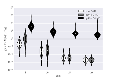
We simulate $T=50$ data-points from the model, for $d=5$, 10, 15 and 20. Figure 2 compares the following four algorithms: SMC-bootstrap, SQMC-bootstrap, SMC-guided, and SQMC-guided. The comparison is in terms of the MSE (mean square error) of the estimate of the filtering expectation of the first component of $X_{t}$, i.e. $\mathbb{E}[X_{t}(1)|Y_{0:t}=y_{0:t}]$. We use SMC-guided as the reference algorithm, and we plot for each of the three other algorithms the variations of the gain (MSE of reference algorithm divided by MSE of considered algorithm) for the $T$ estimates. (We use violin plots, which are similar to box-plots, except that the box is replaced by kernel density estimates.) A gain $g$ means that the considered algorithm would need $g$ times less particles (roughly) to provide an estimate with a similar variance (to that of the reference algorithm). Each algorithm was run with $N=10^{4}$.

Figure 2: Violin plots of the gains of the considered algorithms when estimating the filtering expectations $\mathbb{E}[X_{t}(1)|Y_{0:t}]$ for $t=0,\ldots,T=50$. (Each violin plot represents the variability of the $T$ gains for these $T$ estimates.) Gain is MSE (mean square error) of reference algorithm (guided-SMC) divided by MSE of considered algorithm.

First, we observe that guided algorithms outperforms bootstrap algorithms more and more as the dimension increases. Second, for bootstrap algorithms, the performance between SMC and SQMC is on par as soon as $d\geq 10$. (In fact, the performance is rather bad in both cases, owning to the aforementioned curse of dimensionality.) On the other hand, for guided formalisms we still observe a gain of order $\mathcal{O}(10^{1})$ (resp. $10^{0.5}$) for $d=10$ (resp. $d=20$).

The bottom line is that the amount of extra performance brought by SQMC (relative to SMC) depends strongly on the chosen Feynman-Kac formalism. If one is able to construct a Feynman-Kac formalism (for the considered problem) that leads to good performance for the corresponding SMC algorithm (meaning that the variance of the weights is low at each iteration), then one may expect significant extra performance from SQMC, even in high dimension.

3 Application to Diffusions

3.1 Dimension Reduction in SQMC

We start this section by a basic remark, which makes it possible to improve the performance of SQMC when applied to models having a certain structure. We explained in Section 2.4 that SMC amounts to performing importance sampling at every step, using as a proposal distribution:

$$\sum_{n=1}^{N}W_{t-1}^{n}\delta_{X_{t-1}^{n}}(\mathrm{d}x_{t-1})M_{t}(x_{t-1},\mathrm{d}x_{t})$$ (5)

and as a target distribution, the same distribution times $G_{t}(x_{t-1},x_{t})$ (up to a constant). We used this remark to derive SQMC as an algorithm that constructs a low-discrepancy point-set with respect to the distribution above; i.e. to construct $N$ points $\big{(}X_{t-1}^{A_{t}^{n}},X_{t}^{n}\big{)}$, the empirical distribution of which approximates well (5).

Now consider a situation where we know of a function $\Lambda:{\mathfrak{X}}\rightarrow{\mathbb{R}}^{k}$, with $k<d$, such that (a) $G_{t}$ depends only on $X_{t}$ and $\Lambda(X_{t-1})$; and Markov kernel $M_{t}(x_{t-1},\mathrm{d}x_{t})$ also depends only on $\Lambda(x_{t-1})$. (In particular, it is possible to simulate $X_{t}$ conditional on $X_{t-1}$, knowing only $\Lambda(X_{t-1})$.) In that case, one may define the same importance sampling operation on a lower-dimensional space. In particular, the new proposal distribution would be:

$$\sum_{n=1}^{N}W_{t-1}^{n}\delta_{\Lambda(X_{t-1}^{n})}(\mathrm{d}\lambda_{t-1})M_{t}^{\Lambda}(\lambda_{t-1},\mathrm{d}x_{t})$$

where $M_{t}^{\Lambda}(\lambda_{t-1},\mathrm{d}x_{t})$ is simply the Markov kernel which associates distribution $M_{t}(x_{t-1},\mathrm{d}x_{t})$ to any $x_{t-1}$ such that $\Lambda(x_{t-1})=\lambda_{t-1}$. We may use exactly the same ideas as before, i.e. generate a QMC point of dimension $d+1$, and use the first component to pick the ancestor. However, the Hilbert sorting is now applied to the $N$ points $\Lambda(X_{t-1}^{n})$, and therefore operates in a smaller dimension. Thus one may expect better performance, compared to the standard version of SQMC.

This remark is related somehow to the QMC notion of “effective dimension”: the performance of QMC may remain good in high-dimensional problems, if one is able to reformulate the problem in such a way that it depends “mostly” (or in our case, “only”) on a few dimensions of the state-space.

3.2 Filtering of Diffusion Processes

We now consider the general class of diffusion-driven state-space models:

$$\mathrm{d}\widetilde{X}_{t} =\mu_{X}(\widetilde{X}_{t})+\sigma_{X}(\widetilde{X}_{t})\mathrm{d}W_{t}^{X}$$

$$\mathrm{d}\widetilde{Y}_{t} =\mu_{Y}(\widetilde{X}_{t})+\sigma_{Y}(\widetilde{X}_{t})\mathrm{d}W_{t}^{Y}$$

where ($W_{t}^{X})_{t\geq 0}$ and ($W_{t}^{Y})_{t\geq 0}$ are possibly correlated Wiener processes. Functions $\mu_{X}$, $\mu_{Y}$, $\sigma_{X}$ and $\sigma_{Y}$ may also depend on $t$, and $\mu_{Y}$, $\sigma_{Y}$ may also depend on $Y_{t}$, but for the sake of exposition we stick to the simple notations above.

Filtering in continuous time amounts to recover the distribution of $\widetilde{X}_{t}$ conditional on trajectory $y_{[0:t]}$ (i.e. the observation of process $\{\widetilde{Y}_{t}\}$ over interval $[0,t]$). However, in most practical situations, one does not observe process $\{\widetilde{Y}_{t}\}$ continuously, but on a grid. To simplify, we assume henceforth that process $\{\widetilde{Y}_{t}\}$ is observed at times $t\in\mathbb{N}$ and we rewrite the above model as

$$\mathrm{d}\widetilde{X}_{t} =\mu_{X}(\widetilde{X}_{t})+\sigma_{X}(\widetilde{X}_{t})\mathrm{d}W_{t}^{X}$$

$$\widetilde{Y}_{t+1} =\widetilde{Y}_{t}+\int_{t}^{t+1}\mu_{Y}(\widetilde{X}_{s})\mathrm{d}s+\int_{t}^{t+1}\sigma_{Y}(\widetilde{X}_{s})\mathrm{d}W_{s}^{Y}.$$ (6)

It is typically too difficult to work directly in continuous time. Thus, as standardly done when dealing with such processes, we replace the initial process $(\widetilde{X}_{t})$ by its (Euler-) discretized version $\{X_{t}\}$, with discretisation step $\delta=1/M$, $M\geq 1$. That is, $\left\{X_{t}\right\}$ is a ${\mathbb{R}}^{M}-$valued process, where $X_{t}$ is a $M$-dimensional vector representing the original process at times $t$, $t+1/M$, …, $t+1-1/M$, which is defined as:

$$\begin{split}X_{t}(1)&=X_{t-1}(M)+\delta\mu_{X}\left(X_{t-1}(M)\right)+\sigma_{X}(X_{t-1}(M))\left\{W_{t+\delta}^{X}-W_{t}^{X}\right\}\\ &\vdots\\ X_{t}(M)&=X_{t}(M-1)+\delta\mu_{X}\left(X_{t}(M-1)\right)+\sigma_{X}(X_{t}(M-1))\left\{W_{t+1}^{X}-W_{t+1-\delta}^{X}\right\}\end{split}$$ (7)

and the resulting dicretization of (6) is given by

$$Y_{t+1}=Y_{t}+\delta\sum_{m=1}^{M}\mu_{Y}\left(X_{t}(m)\right)+\sum_{m=1}^{M}\sigma_{Y}\left(X_{t}(m)\right)\big{\{}W_{t+\delta m}^{Y}-W_{t+\delta(m-1)}^{Y}\big{\}}.$$ (8)

SQMC may be applied straightforwardly to the filtering of the discretized model defined by (7) and (8). However, the choice of the $\delta=1/M$ becomes problematic. We would like to take $M$ large, to reduce the discretization bias. But $M$ is also the dimension of the state-space, so a large $M$ may mean a degradation of performance for SQMC (relative to SMC).

Fortunately, the dimension reduction trick of the previous section applies here. For simplicity, consider the bootstrap Feynman-Kac formalism of this particular state-space model:

• $M_{t}(x_{t-1},\mathrm{d}x_{t})$ is the distribution of $X_{t}|X_{t-1}$ defined by (7); observe that it only depends on $X_{t-1}(M)$, the last component of $X_{t-1}$;

• $G_{t}(x_{t-1},x_{t})$ is the probability density of datapoint $y_{t}$ given $X_{t}=x_{t}$ and $Y_{t-1}=y_{t-1}$, induced by (7)-(8); observe that it does not depend on $x_{t-1}$ when $(W^{X}_{t})$ and $(W^{Y}_{t})$ are uncorrelated and that it depends on $x_{t-1}$ only through $x_{t-1}(M)$ when these two processes are correlated (see the next subsection).

Hence we may define $\Lambda(x_{t-1})=x_{t-1}(M)\in{\mathbb{R}}$. The Hilbert ordering step may be applied to the values $Z_{t}^{n}=X_{t-1}^{n}(M)$. In fact, since these values are scalars, there is no need to implement any Hilbert ordering, a standard sorting is enough.

3.3 QMC and Brownian Motion

We now briefly discuss how to choose $\Gamma_{t}$, the deterministic function such that $\Gamma_{t}(x_{t-1},v)$, for $x_{t-1}\in{\mathfrak{X}}$ and $v\in[0,1]^{d}$, returns a variate from kernel $M_{t}(x_{t-1},\mathrm{d}x_{t})$.

The distribution of $X_{t}|X_{t-1}$ defined in the previous section is a simple linear transform of the distribution of a Brownian path on a regular grid. Thus, defining function $\Gamma_{t}$ amounts to constructing a certain function $[0,1]^{M}\rightarrow{\mathbb{R}}^{M}$ that transforms $\mathcal{U}\left([0,1]^{M}\right)$ into the joint distribution of $(W^{X}_{t+\delta},\ldots,W^{X}_{t+1})$, conditional on $W^{X}_{t}$.

It is well known in the QMC literature (e.g. Section 8.2 of MR3289176 ) that there is more than one way to write the simulation of a Brownian path as a function of uniforms, and that the most obvious way may perform poorly when applied in conjunction with QMC. More precisely, consider the following two approaches:

1. Forward construction: simulate independently the increments $W^{X}_{t+\delta m}-W^{X}_{t+\delta(m-1)}$ from a $N(0,\delta)$ distribution.

2. Brownian bridge construction Caflisch1997 : Simulate $(W^{X}_{t+\delta},\dots,W^{X}_{t+1})$ given $W^{X}_{t}$ sequentially according to the Van der Corput sequence: $W_{t+\delta\lceil M/2\rceil}^{X}$, $W_{t+\delta\lceil M/4\rceil}^{X}$, $W_{t+\delta\lceil 3M/4\rceil}^{X}$ until all the components of vector $(W^{X}_{t+\delta},\ldots,W^{X}_{t+1})$ are simulated. For instance, for $s<t^{\prime}<u$, we use

   $$W_{t^{\prime}}^{X}|W_{s}^{X},W_{u}^{X}\sim N_{1}\left(\frac{u-t^{\prime}}{u-s}W_{s}^{X}+\frac{t^{\prime}-s}{u-s}W_{u}^{X},\frac{(u-t^{\prime})(t^{\prime}-s)}{u-s}\right)$$

   and the fact that $(W_{t}^{X})$ is a Markov process (i.e. $W_{t}^{X}|W_{s}^{X}$ does not depend on $W_{s^{\prime}}^{X}$ for $s^{\prime}<s$).

In both cases, it is easy to write the simulation of $(W^{X}_{t+\delta},\ldots,W^{X}_{t+1})$ as a function of $M$ uniform variates. However, in the first case, the obtained function depends in the same way on each of the $M$ variates, while in the second case, the function depends less and less on the successive components. This mitigates the inherent curse of dimensionality of QMC Caflisch1997 .

We shall observe the same phenomenon applies to SQMC; even so for a moderate value of $M$, interestingly. We also mention briefly the PCA (principal components analysis) construction as another interesting way to construct Brownian paths, and refer again to Section 8.2 MR3289176 for a more in-depth discussion of QMC and Brownian paths.

Lastly, although we focus on univariate diffusion processes in this section for the sake of simplicity, the above considerations also hold for multivariate models. Notably, the Brownian bridge construction is easily generalizable to the case where $(W^{X}_{t})$ is a $d$-dimensional vector of correlated Wiener processes. The dimension of the QMC point set used as input of SQMC is then of size $dM+1$ and the Hilbert ordering would operate on a $d$-dimensional space.

3.4 Numerical Experiments

To illustrate the discussion of the previous subsections we consider the following diffusion driven stochastic volatility model (e.g.Chib2004 )

$$\mathrm{d}\widetilde{X}_{t} =\Big{\{}\kappa(\mu^{X}-e^{\widetilde{X}_{t}})e^{-\widetilde{X}_{t}}-0.5\omega^{2}e^{-X_{t}}\Big{\}}\mathrm{d}t+\omega e^{-\widetilde{X}_{t}/2}\mathrm{d}W^{X}_{t}$$

$$\widetilde{Y}_{t+1} =\widetilde{Y}_{t}+\int_{t}^{t+1}\big{\{}\mu^{Y}+\beta e^{\widetilde{X}_{z}}\big{\}}\mathrm{d}z+\int_{t}^{t+1}e^{\widetilde{X}_{s}/2}\mathrm{d}W_{s}^{Y}$$

where $(W^{X}_{t})$ and $(W^{Y}_{t})$ are Wiener processes with correlation coefficient $\rho\in(-1,1)$, $\omega>0$, $\kappa>0$ while the other parameters $\mu^{Y}$, $\beta$ are in ${\mathbb{R}}$.

To fit this model into the bootstrap Feynman-Kac formalism that we consider in this section, note that, for $t\geq 0$,

$$\widetilde{Y}_{t+1}|\widetilde{Y}_{t},\widetilde{X}_{[t,t+1]}\sim N\Big{(}\widetilde{Y}_{t}+\mu^{Y}+\beta\sigma_{t+1}^{2}+\rho Z_{t+1},\,\,(1-\rho^{2})\sigma_{t+1}^{2}\Big{)}$$

with $\sigma_{t+1}^{2}=\int_{t}^{t+1}e^{\widetilde{X}_{s}}\mathrm{d}s$ and $Z_{t+1}=\int_{t}^{t+1}e^{\widetilde{X}_{s}/2}\mathrm{d}W^{X}_{s}$, and thus, as explained in Section 3.2,

$$\begin{split}G_{t}(x_{t-1},x_{t})&=\tilde{G}_{t}(x_{t-1}(M),x_{t})\\ &:=N\Big{(}\widetilde{Y}_{t+1};\widetilde{Y}_{t}+\mu^{Y}+\beta\hat{\sigma}_{t+1}^{2}(x_{t})+\rho\hat{Z}_{t+1}(x_{t-1}(M),x_{t}),\,\,(1-\rho^{2})\hat{\sigma}_{t+1}^{2}(x_{t})\Big{)}\end{split}$$

where

$$\hat{\sigma}_{t+1}^{2}(x_{t})=\frac{1}{M}\sum_{m=1}^{M}e^{x_{t}(m)},\quad\hat{Z}_{t+1}(x_{t-1}(M),x_{t})=\sum_{m=1}^{M}e^{\frac{x_{t}(m)}{2}}\big{(}W^{X}_{t+m\delta}-W^{X}_{t+(m-1)\delta}\big{)}.$$

Note that $W^{X}_{t+m\delta}-W^{X}_{t+(m-1)\delta}$ depends on $(x_{t-1}(M),x_{t})$ through (7). To complete the model we take for $\mathbb{M}_{0}(\mathrm{d}x_{0})$, the initial distribution of process $\{X_{t}\}$, the density of the $N\big{(}\mu^{X},\omega^{2}/(2\kappa)\big{)}$ distribution.

We set the parameters of the model to their estimated values for the daily return data on the closing price of the S&P 500 index from 5/5/1995 to 4/14/2003 Chib2004 and simulate observations $\{Y_{t}\}_{t=0}^{T}$ using the discretized model (7)-(8) with $M=20\,000$. The number of observations $T$ is set to $4\,000$.

Below we compare SMC with SQMC based on the forward construction and on the Brownian bridge construction of Brownian paths. In both cases, SQMC is implemented using as input a nested scrambled Owen1995 Sobol’ sequence. The performance of these three algorithms is compared, for $t=1,\dots,T$, for the estimation of (1) the filtering expectation $\mathbb{E}[X_{t}|Y_{0:t}]$ and (2) of the log-likelihood function $\log(L_{t})$.

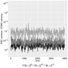
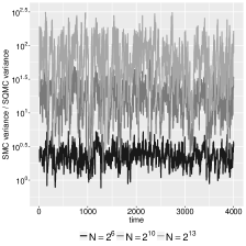
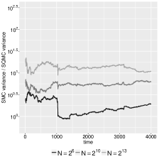
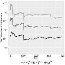
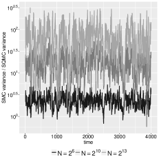
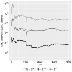
Figure 3 shows the ratio of the SMC variance over the SQMC variance for the two alternative implementations of SQMC. Results are presented for a discretization grid of size $M=5$ and for different number of particles $N$. Two observations are worth noting from this figure. First, the two versions of SQMC outperform SMC in terms of variance. Second, the variance reduction is much larger with the Brownian bridge construction than with the forward construction of Brownian paths, as expected from the discussion of the previous subsection. Note that for both versions of SQMC the ratio of variances increases with the number of particles, showing that SQMC converges faster than the $N^{-1/2}$ Monte Carlo error rate.

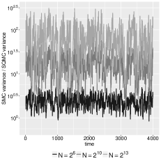
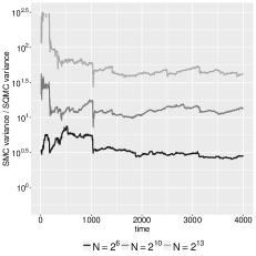
In Figure 4 we perform the same analysis than in Figure 3 but now with $M=10$ and $M=20$ discretization steps. ($M=10$ is considered as sufficient for parameter estimation by Chib2004 .) Results are presented only for the Brownian bridge construction. Despite the large dimension of the QMC point set used as input, we observe that SQMC converges much faster than the $N^{-1/2}$ Monte Carlo error rate. In particular, we observe that the gains in term of variance brought by SQMC are roughly similar whatever the choice of $M$ is. As explained above, this observation suggests that the effective dimension of the model remains low (or even constant in the present setting) even when the “true” dimension $M$ increases.

Figure 3: Estimation of $\mathbb{E}[X_{t}|Y_{0:t}=y_{0:t}]$ (top plots) and of $\log p(y_{0:t})$ for $t\in\{0,\dots,T\}$ and for different values of $N$. SQMC is implemented with the forward construction (left plots) and with the Brownian Bridge construction of Brownian paths (right plots), and $M=5$

Figure 4: Estimation of $\mathbb{E}[X_{t}|Y_{0:t}=y_{0:t}]$ (top) and of $\log p(y_{0:t})$ for $t\in\{0,\dots,T\}$ and for different values of $N$. SQMC is implemented with the Brownian Bridge construction of Brownian paths. Results are presented for $M=10$ (left plots) and for $M=20$.

Resampling

Algorithm 4 below takes as input $N$ sorted points $u^{1}\leq\ldots\leq u^{n}$, and $N$ weights $W^{n}$, and return as an output the $N$ values $\left(F^{N}\right)^{-1}(u^{n})$, where $\left(F^{N}\right)^{-1}$ is the inverse CDF relative to CDF $F^{N}(z)=\sum_{n=1}^{N}W^{n}{\mathbbold{1}}\{n\leq z\}$, $z\in{\mathbb{R}}$. Its complexity is $O(N)$.

To compute the inverse CDF corresponding to the empirical CDF of $N$ ancestors (as discussed in Section 2.6), i.e.

$$F^{N}(x)=\sum_{n=1}^{N}W^{n}{\mathbbold{1}}\left\{X^{n}\leq x\right\}$$

simply order the $N$ ancestors, and apply the same algorithm to the sorted ancestors.

Algorithm 4 Resampling Algorithm (inverse transform method)

Input: $u^{1:N}$ (such that $0\leq u^{1}\leq\ldots\leq u^{N}\leq 1$, $W^{1:N}$ (normalised weights)
Output: $a^{1:N}$ (labels in $1:N$)

$s\leftarrow 0$, $m\leftarrow 0$

for $n=1\to N$ do

repeat

$m\leftarrow m+1$

$s\leftarrow s+W^{m}$

until $s>u^{n}$

$a^{n}\leftarrow m$

end for

References

• (1) Andrieu, C., Doucet, A., Holenstein, R.: Particle Markov chain Monte Carlo methods. J. R. Stat. Soc. Ser. B Stat. Methodol. 72(3), 269–342 (2010). DOI 10.1111/j.1467-9868.2009.00736.x
• (2) Arulampalam, M.S., Maskell, S., Gordon, N., Clapp, T.: A tutorial on particle filters for online nonlinear/non-gaussian Bayesian tracking. IEEE Transactions on signal processing 50(2), 174–188 (2002)
• (3) Briers, M., Doucet, A., Maskell, S.: Smoothing algorithms for state-space models. Ann. Inst. Statist. Math. 62(1), 61–89 (2010). DOI 10.1007/s10463-009-0236-2
• (4) Caflisch, R.E., Morokoff, W.J., Owen, A.B.: Valuation of mortgage backed securities using Brownian bridges to reduce effective dimension. Department of Mathematics, University of California, Los Angeles (1997)
• (5) Chib, S., Pitt, M.K., N., S.: Likelihood-based inference for diffusion models. Tech. rep., Nuffield College, Oxford (2004)
• (6) Chopin, N.: A sequential particle filter method for static models. Biometrika 89(3), 539–551 (2002). DOI 10.1093/biomet/89.3.539
• (7) Chopin, N.: Central limit theorem for sequential Monte Carlo methods and its application to Bayesian inference. Ann. Statist. 32(6), 2385–2411 (2004). DOI 10.1214/009053604000000698
• (8) Del Moral, P.: Non-linear filtering: interacting particle resolution. Markov processes and related fields 2(4), 555–581 (1996)
• (9) Del Moral, P., Doucet, A., Jasra, A.: Sequential Monte Carlo samplers. J. R. Stat. Soc. Ser. B Stat. Methodol. 68(3), 411–436 (2006). DOI 10.1111/j.1467-9868.2006.00553.x
• (10) Del Moral, P., Guionnet, A.: Central limit theorem for nonlinear filtering and interacting particle systems. Ann. Appl. Probab. 9(2), 275–297 (1999). DOI 10.1214/aoap/1029962742
• (11) Doucet, A., de Freitas, N., Gordon, N.J.: Sequential Monte Carlo Methods in Practice. Springer-Verlag, New York (2001)
• (12) Doucet, A., Godsill, S., Andrieu, C.: On sequential Monte Carlo sampling methods for Bayesian filtering. Statist. Comput. 10(3), 197–208 (2000). DOI 10.1023/A:1008935410038
• (13) Doucet, A., Kantas, N., Singh, S.S., Maciejowski, J.M.: An overview of Sequential Monte Carlo methods for parameter estimation in general state-space models. In: Proceedings IFAC System Identification (SySid) Meeting. (2009)
• (14) Fearnhead, P.: Using random quasi-Monte-Carlo within particle filters, with application to financial time series. J. Comput. Graph. Statist. 14(4), 751–769 (2005). DOI 10.1198/106186005X77243
• (15) Gerber, M., Chopin, N.: Convergence of Sequential Quasi-Monte Carlo Smoothing Algorithms. ArXiv preprint 1506.06117 (2015)
• (16) Gerber, M., Chopin, N.: Sequential quasi Monte Carlo. J. R. Stat. Soc. Ser. B. Stat. Methodol. 77(3), 509–579 (2015). DOI 10.1111/rssb.12104
• (17) Guarniero, P., Johansen, A.M., Lee, A.: The iterated auxiliary particle filter. ArXiv e-prints (2015)
• (18) Kalman, R.E., Bucy, R.S.: New results in linear filtering and prediction theory. Trans. ASME Ser. D. J. Basic Engrg. 83, 95–108 (1961). DOI 10.1115/1.3658902
• (19) Kim, S., Shephard, N., Chib, S.: Stochastic volatility: likelihood inference and comparison with arch models. The Review of Economic Studies 65(3), 361–393 (1998)
• (20) L’Ecuyer, P., Lécot, C., Tuffin, B.: A randomized quasi-Monte Carlo simulation method for Markov chain. In: Monte-Carlo and quasi Monte-Carlo methods 2004, pp. 331–342. Springer Berlin Heidelberg (2006)
• (21) Lemieux, C.: Monte Carlo and Quasi-Monte Carlo Sampling (Springer Series in Statistics). Springer (2009)
• (22) Leobacher, G., Pillichshammer, F.: Introduction to quasi-Monte Carlo integration and applications. Compact Textbook in Mathematics. Birkhäuser/Springer, Cham (2014). DOI 10.1007/978-3-319-03425-6
• (23) Neal, R.M.: Annealed importance sampling. Stat. Comput. 11(2), 125–139 (2001). DOI 10.1023/A:1008923215028
• (24) Owen, A.B.: Randomly permuted (t,m,s)𝑡𝑚𝑠(t,m,s)-nets and (t,s)𝑡𝑠(t,s)-sequences. In: Monte Carlo and Quasi-Monte Carlo Methods in Scientific Computing. Lecture Notes in Statististics, vol. 106, pp. 299–317. Springer, New York (1995)
• (25) Pitt, M.K., Shephard, N.: Filtering via simulation: auxiliary particle filters. J. Amer. Statist. Assoc. 94(446), 590–599 (1999). DOI 10.2307/2670179
Resampling
Algorithm 4 below takes as input N𝑁N sorted points u1unsuperscript𝑢1superscript𝑢𝑛u^{1}\leq\ldots\leq u^{n}, and N𝑁N weights Wnsuperscript𝑊𝑛W^{n}, and return as an output the N𝑁N values (FN)1(un)superscriptsuperscript𝐹𝑁1superscript𝑢𝑛\left(F^{N}\right)^{-1}(u^{n}), where (FN)1superscriptsuperscript𝐹𝑁1\left(F^{N}\right)^{-1} is the inverse CDF relative to CDF FN(z)=n=1NWn1{nz}superscript𝐹𝑁𝑧superscriptsubscript𝑛1𝑁superscript𝑊𝑛1𝑛𝑧F^{N}(z)=\sum_{n=1}^{N}W^{n}{\mathbbold{1}}\{n\leq z\}, z𝑧z\in{\mathbb{R}}. Its complexity is O(N)𝑂𝑁O(N).