Solvable models of an open well and a bottomless barrier: 1-D potentials

Abstract

We present one dimensional potentials $V(x)=V_{0}[e^{2|x|/a}-1]$ as solvable models of a well $(V_{0}>0)$ and a barrier ($V_{0}<0$). Apart from being new addition to solvable models, these models are instructive for finding bound and scattering states from the analytic solutions of Schrödinger equation. The exact analytic (semi-classical and quantal) forms for bound states of the well and reflection/transmission $(R/T)$ coefficients for the barrier have been derived. Interestingly, the crossover energy $E_{c}$ where $R(E_{c})=1/2=T(E_{c})$ may occur below/above or at the barrier-top. A connection between poles of these coefficients and bound state eigenvalues of the well has also been demonstrated.

I Introduction

Solutions of Schrödinger equation arising from dimensional potentials have been enriching the understanding of microscopic world through quantum mechanics [1-5]. At the heart of Planck’s explanation of black body radiation and the Einstein’s theory of specific heat of solids there lies the harmonic oscillator potential $V(x)=\frac{1}{2}\mu\omega^{2}x^{2}$ and its discrete bound state spectrum $(n+1/2)\hbar\omega$. Transmission across a triangular potential barrier explains cold emission of electrons from metals through Fowler-Nordheim factor. Tunneling through a parabolic barrier could explain nuclear fusion cross-sections. Transmission at a simple rectangular barrier is Gamow’s model of $\alpha$ decay from nucleus. In microscopic world, the success story of one dimensional potential wells and barriers, which have one minimum and one maximum respectively is most interesting.

However, there are only few potential functions which are amenable to exact analytic solutions. Textbooks discuss potentials like Dirac-Delta [1], rectangular (square) [1-4], parabolic [4,5], triangular [5], Eckart [3,4], Fermi-step [3,4] and Rosen-Morse [6] potentials. The exact solvability of Scarf II [7] and the versatile Ginocchio’s potential [8] has come up rather late. The Exponential potential $V(x)=-V_{0}e^{x/a}$ has been suggested [10] as a simple practice problem that gives rise to the simplest forms for reflection $R(E)$ and transmission $T(E)$ coefficients. The Morse [11] and one more potential barrier [12] have been presented giving rise to simple analytic expressions for $T(E)$ and $R(E)$. Symmetric exponential [9], bi-harmonic [13] and symmetric triangular [5] potentials have been solved in terms of higher order functions, like Bessel, parabolic cylindrical and Airy functions. These models are even more welcome now, as various packages can calculate higher order functions fast and accurate. Though quick numerical algorithms of integration of Schödinger equation are also available yet handing higher order functions to extract bound and scattering states analytically or semi-analytically cannot loose its charm and importance specially when potentials diverge to $\pm\infty$ as $|x|\rightarrow\infty.$ This is so because for scattering states, asymptotic boundary conditions cannot be put unless the Schrödinger equation is analytically solvable.

The alternate quantum mechanical approaches like super symmetric methods [14,15] have furthered the pursuit of exactly solvable models remarkably. Very interesting analytic forms [16,17] of complex scattering amplitudes $r(k)$ and $t(k)$ for Scarf II have emerged from such studies. Simplified form of $T(E)$ for this case is also available [18].

In this paper, we wish to introduce the exponential potential

$$V(x)=V_{0}(e^{2|x|/a}-1),$$ (1)

When $V_{0}>0$, it is an open well which diverges to $\infty$ as $|x|\rightarrow\infty$, see Fig 1(a). When $V_{0}<0$ it represents a bottomless potential barrier (Fig. 1(b)). In the following, we discuss the extraction of bound state eigenfunctions and eigenvalues and extraction of scattering states giving rise to reflection $r(k)$ and transmission $t(k)$ amplitudes from exact analytic solutions of Schrödinger equation. We also find them by using the semi-classical approximation called WKB method. An instructive connection of bound state eigenvalues with the poles of the reflection and transmission coefficients will also be discussed.

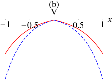
Figure 1: Plots of the exponential potentials: (a) the open well (Eq.(1), $V_{0}=1$) and (b) the bottomless barrier (Eq.(8), $U0=1)$. For the length parameter $a=1$ see red/solid lines and for $a=0.8$ see blue/dashed, for larger values of $a$ these potentials are thicker. The open well has only discrete positive energies as bound state eigenvalues. The barrier has only scattering states at both positive and negative values.

II Boundstates in the open well

We write the Schrodinger equation for (1) as

$$\frac{d^{2}\psi(x)}{dx^{2}}+[k^{2}-q^{2}e^{2|x|/a}]\psi(x)=0,\quad k=\sqrt{2\mu(E+V_{0})}/\hbar,\quad q=\sqrt{2\mu V_{0}}/\hbar.$$ (2)

By using the transformation $z=\lambda e^{|x|/a}$ [19] in (2) we can transform it to modified Bessel equation [20] as

$$z^{2}\frac{d^{2}\psi(z)}{dz^{2}}+z\frac{d\psi(z)}{dz}-(\nu^{2}+z^{2})\psi(z)=0,\quad\nu=ika,\quad\lambda=qa.$$ (3)

This second order equation is known to have two linearly dependent solutions as $I_{\nu}(z)$ and $K_{\nu}(z)$. Despite $\nu=ika$ being imaginary both $I_{\pm ika}(\lambda e^{|x|/a})$ [20] are real continuous functions of $x$. When $x$ and so $z$ is large $I_{\nu}(z)$ diverges $\sim\frac{e^{z}}{\sqrt{2\pi z}}$ but $K_{\nu}(z)$ converges to zero as $\sim\frac{e^{-z}}{\sqrt{2\pi z}}$. Thus, it is the second solution that satisfies Dirichlet condition that $\psi(\pm\infty)=0$. Since the potential (1) is symmetric, the Eq. (2,3) will have definite parity even/odd solutions. The even parity solution is

$$\psi_{e}(x)=AK_{ik_{n}a}(qae^{|x|/a}),\quad K^{\prime}_{ik_{n}a}(qa)=0,\quad n=0,2,4,...$$ (4)

The condition that $K^{\prime}_{ik_{n}a}(qa)=0$ quantizes energy $E=k^{2}_{n}$ and ensures the differentiability of $\psi(x)$ at $x=0$ despite $|x|$ being there. The odd parity solution is given as

$$\psi_{o}(x)=A~{}\mbox{sgn}(x)~{}K_{ik_{n}a}(qae^{|x|/a}),\quad K_{ik_{n}a}(qa)=0,\quad n=1,3,5,...$$ (5)

The condition that $K_{ik_{n}a}(qa)=0$ quantizes energy $E=k^{2}_{n}$ and ensures that these (odd) eigenfunction vanish essentially at $x=0$. Eqs (4) and (5) give complete spectrum of the open well which has infinite number of eigenvalues.

For a demonstration of first four bound states of the well, let us take $V_{1}=1,a=1$ in arbitrary units where $2\mu=1=\hbar^{2}$ for convenience. This choice corresponds to a particle whose mass is roughly 4 times that of mass of electron; mass/energy and length are measured in eV and $A^{0}$ (Angstrom), respectively. This choice also corresponds to a particle whose mass is roughly 20 times that of proton or neutron when mass/energy and length are measured in MeV and fm (Fermi), respectively.

We plot $K_{ik}(1)$ and $K_{ik}^{\prime}(1)$ ($qa=1$) as a function of $E$ where $k=\sqrt{E+1}$ to find that these functions pass through zero roughly around $E\sim 2,13$ and $E\sim 8,19$, respectively. Next, we find exact roots by using “FindRoot” of “mathematica” using these four rough guess values. We find the exact eigenvalues are $E_{0}=2.6759$ and $E_{2}=13.3305$ for even states with nodes as 0 and 2, respectively. The exact eigenvalues of odd states as $E_{1}=7.7766$ and $E_{3}=19.5616$ having 1 and 3 nodes, respectively. These four eigenstates are plotted in Fig. 2. Students will find it interesting to check these eigenvalues and eigenstates by using a simple one line “mathematica” program called “wag-the-dog” method (see Problem 2.54 on page 104 in Ref. [1]) for symmetric potential wells.

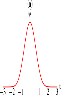
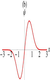
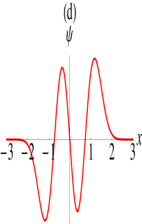
Figure 2: First four (a-d) un-normalized definite parity bound state eigenfunctions (4,5) for the open well (1) are shown. The corresponding energy eigenvalues are $E_{0}=2.6759,E_{1}=7.7766,E_{2}=13.3305$ and $E_{3}=19.5616$

III Bound state eigenvalues by semi-classical quantization

A potential well $V(x)$ having a minimum and two real classical turning points $x_{1}(E),x_{2}(E)$ at positive/negative energies may have real discrete eigenvalues provided

$$\frac{1}{\pi}\int_{x_{1}(E)}^{x_{2}(E)}\sqrt{2\mu[E-V(x)]}dx=(n+1/2)~{}\hbar,\quad n=0,1,2,3...,V(x_{1})=E=V(x_{2}).$$ (6)

Eq. (6) is known as Bohr-Sommerfeld phase space quantization ($n$ in place of $n+1/2$) later it has been derived from Schrödinger equation and it is known as WKB approximation [1-5] for bound state eigenvalues. For the potential well (1) $x_{1,2}=\pm\frac{1}{2}\log[(E+V_{0})/V_{0}]$ and the integral (6) can be performed to give

$$f(E)=\frac{2qag}{\pi}\left(\tanh^{-1}\frac{\sqrt{g^{2}-1}}{g}-\frac{\sqrt{g^{2}-1}}{g}\right)=(n+1/2),\quad g=\sqrt{(E+V_{0})/V_{0}}.$$ (7)

In Fig. 3, $f(E)$ has been plotted along with horizontal lines at $f=0.5,1.5,2.5,3.5$

Figure 3: $f(E)$ (7) plotted for $V_{0}=1$ and $a=1$, $f=0.5,1.5,2.5,3.5$ cut x-axis at $E=2.6471,7.6486,13.2651$ and $19.4743$, these semi-classical eigenvalues lie very close to the exact ones listed in Fig. 2

which cut the energy axis at $2.6471,7.6486,13.2651,19.4743$. These are first four semi classical eigenvalues which are for the case $V_{0}=1$ and $a=1$. It can be seen that they lie very close to $E_{0},E_{1},E_{2},E_{3}$ obtained above using the exact quantum condition (4,5) for bound states.

IV Scattering states in bottomless barrier

The bottomless exponential potential barrier can be written as

$$V(x)=-U_{0}(e^{2|x|/a}-1),\quad U_{0}>0,$$ (8)

see Fig 1(b). $E=0$ marks the top of the barrier so this potential has only scattering states at both positive and negative energies. The Schrödinger equation for this potential is written as

$$\frac{d^{2}\psi(x)}{dx^{2}}+[p^{2}+s^{2}e^{2|x|/a}]\psi(x)=0,\quad p=\sqrt{2\mu(E-U_{0})}/\hbar,\quad s=\sqrt{2\mu U_{0}}/\hbar.$$ (9)

Again using the transformation $z=\lambda e^{|x|/a}$ [19] in (9) we can transform it to modified Bessel equation as

$$z^{2}\frac{d^{2}\psi(z)}{dz^{2}}+z\frac{d\psi(z)}{dz}+(-\nu^{2}+z^{2})\psi(z)=0,\quad\nu=ipa,\quad\lambda=sa.$$ (10)

This cylindrical Bessel equation whose two pairs of linearly independent solutions are $J_{\pm\nu}(z)$ and the Hankel functions $H^{(1)}_{\nu}(z)$ and $H^{(2)}_{\nu}(z)$ [20], any member of these pairs can be expressed as a linear combination of other two. However the latter pair is directly useful since for large values of $x$ or $z$ the Hankel functions [20] behave as scattering states:

$$H^{(1,2)}_{\nu}(z)\sim\sqrt{2/(\pi z)}e^{\pm i(z-i\nu\pi/2-\pi/4)}.$$ (11)

For our potential barrier Fig. 1(b), when the potential is real the scattering is independent of the direction of the incidence of a particle or wave at the potential. So without a loss of generality let us choose the direction of incidence from left. Thus, for scattering from left the incident, reflected and transmitted are to be chosen from $\psi_{1}(x)=H^{(2)}_{ipa}(sae^{-x/a})$, $\psi_{2}(x)=H^{(1)}_{ipa}(sae^{-x/a})$ and $\psi_{3}(x)=H^{(1)}_{ipa}(sae^{x/a})$. For a scattering solution $\psi(x)=\alpha(x)e^{i\beta(x)}$ the time dependent state is written as $\Psi(x,t)=\alpha(x)e^{-i\Phi(x,t)}=\alpha(x)e^{i(\beta(x)-Et/\hbar)}$. Then the sign of the phase velocity $dx/dt$ determined by the condition of stationary phase $\frac{d\Phi(x,t)}{dt}=0$ at an asymptotic distance decides the relative direction of running of these waves arising from solutions $\Psi_{m}(x,t)(m=1,2,3)$. So using (11) let us write the asymptotic forms as

$$\Psi_{1}(x,t) \sim \sqrt{2/(\pi z)}e^{i[-sae^{-x}-Et/\hbar]}\Rightarrow dx/dt>0,\Psi_{2}(x,t)\sim\sqrt{2/(\pi z)}e^{i[sae^{-x}-Et/\hbar]}\Rightarrow dx/dt<0,$$

$$\Psi_{3}(x,t) \sim \sqrt{2/(\pi z)}e^{i[sae^{x}-Et/\hbar]}\Rightarrow dx/dt>0.$$ (12)

Therefore $\Psi_{1}$, $\Psi_{3}$ represent waves moving left to right to be designated as incident $\psi_{i}(x)$ and transmitted $\psi_{t}(x)$ waves, respectively. The reflected wave needs to be traveling opposite to the incident wave and also it should be time reversed (complex conjugate) form of the incident wave, so we choose $\psi_{2}(x)=H^{(1)}_{-ipa}(sa)$ (notice - sign in the subscript) as reflected $\psi_{r}(x)$ wave.

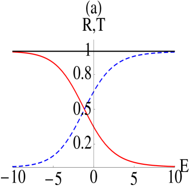
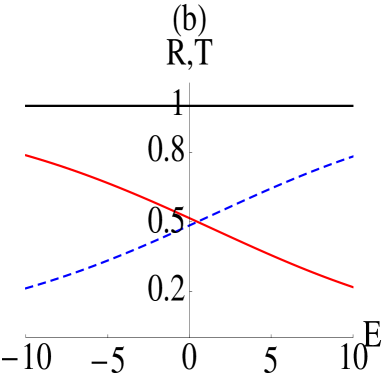
Figure 4: The reflection $R(E)$ (red/solid) and transmission $T(E)$ (blue/dashed) probabilities as a function of energy (15,19) when a particle or wave is incident on the unbounded potential barrier (8) ($U_{0}=5$ and (a): $a=1$, (b) $a=0.2$). The cross-over $R=T=1/2$ occurs at $E=-1.1487<0$. Normally this result is expected at energy equal to the top of the barrier namely $E=0$. However for low values of the effective parameter $qa$ the cross over between $R(E)$ and $T(E)$ can be made to occur at zero or positive energies for instance if $a=0.2$, the crossover occurs at $E=0.4886>0.$ See part (b).

Note that $[H^{(2)}_{i\nu}(z)]^{*}=H^{(1)}_{-i\nu}(z)$ [20]. We can now write the full solution of (9) as

$$\psi(x<0)=AH^{(2)}_{ipa}(sae^{-x/a})+BH^{(1)}_{-ipa}(sae^{-x/a}),\quad\psi(x>0)=CH^{(1)}_{ipa}(sae^{x/a}).$$ (13)

The condition of continuity and differentiability of $\psi(x)$ everywhere demands the above two pieces of solutions to be continuous and and differentiable at $x=0$. So we get

$$AH^{(2)}_{ipa}(sa)+BH^{(1)}_{-ipa}(sa)=CH^{(1)}_{ipa}(sa),\quad AH^{(2)^{\prime}}_{ipa}(sa)+BH^{(1)^{\prime}}_{-ipa}(sa)=-CH^{(1)^{\prime}}_{ipa}(sa)$$ (14)

We get expressions of A,B and C by solving (14). We get $A=2H^{(1)}_{-ipa}(sa)H^{(1)^{\prime}}_{ipa}(sa)$, $B=H^{(1)^{\prime}}_{ipa}(sa)H^{(2)}_{ipa}(sa)+H^{(1)}_{ipa}(sa)H^{(2)^{\prime}}_{ipa}(sa)$, $C=H^{(1)}_{-ipa}(sa)H^{(2)^{\prime}}_{ipa}(sa)-H^{(1)^{\prime}}_{-ipa}(sa)H^{(2)}_{ipa}(sa).$ Consequently the ratios $B/A$ and $C/A$ turns out to be are obtained as

$$\frac{B}{A} = -\frac{1}{2}e^{\pi pa}\left[\frac{H^{(2)}_{ipa}(sa)}{H^{(1)}_{ipa}(sa)}+\frac{H^{(2)^{\prime}}_{ipa}(sa)}{H^{(1)^{\prime}}_{ipa}(sa)}\right]$$

$$\frac{C}{A} = \frac{2i/(\pi sa)}{H^{(1)}_{ipa}(sa)~{}H^{(1)^{\prime}}_{ipa}(sa)}.$$ (15)

In above, we have used the properties that $H^{(1)}_{-\nu}(z)=e^{i\pi\nu}H^{(1)}_{\nu}(z)$, $H^{(2)}_{-\nu}(z)=e^{-i\pi\nu}H^{(2)}_{\nu}(z)$ and $[H^{(1)}_{\nu}(z)H^{(2)^{\prime}}_{\nu}(z)-H^{(1)^{\prime}}_{\nu}(z)H^{(2)}_{\nu}(z)]=-4i/(\pi z)[20].$ These properties also help in calculating the current density [1-5]

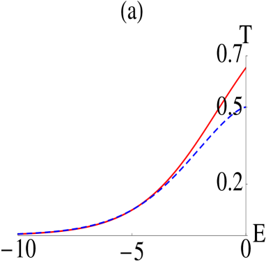
Figure 5: Exact (Eqs. (15,19), solid) and WKB (Eq.(21), dashed) transmission probabilities for (a): $U_{0}=5,a=1$, (b): $U_{0}=5,a=0.2.$ In (a) $T(0)>T_{WKB}(0)=1/2$ and in (b) $T(0)<T_{WKB}(0)=1/2.$ $E=0$, marks the barrier-top

$${\cal J}=\frac{\hbar}{2i\mu}[\psi^{*}(x)\psi^{\prime}(x)-\psi(x)\psi^{*^{\prime}}(x)]$$ (16)

easily on the left and right due to $\psi(x)$ in (13). We get when $p$ is purely imaginary

$${\cal J}_{<}={\cal J}_{0}(AA^{*}-BB^{*}),\quad\mbox{and},\quad{\cal J}_{>}={\cal J}_{0}CC^{*},\quad{\cal J}_{0}=\frac{2\hbar}{\mu a\pi},$$ (17)

on the left and the right of $x=0$. But when $p$ is real, we get

$${\cal J}_{<}={\cal J}_{0}e^{-\pi pa}(AA^{*}-BB^{*}),\quad{\cal J}>={\cal J}_{0}e^{\pi pa}CC^{*},$$ (18)

on the left and right of $x=0$. The conservation of particle flux at or continuity of current density $x=0$ is met as $1-R(E)=T(E)$, where $R(E)$ and $T(E)$ reflection and transmission probabilities of the particle incident at the barrier (8). Thus $R(E)$ and $T(E)$ for the barrier (8) can be given commonly as

$$R(E)=\left|\frac{B}{A}\right|^{2},\quad T(E)=\left|e^{\pi pa}\frac{C}{A}\right|^{2},$$ (19)

where we use the results in eq. (15). Alternatively simpler way is to calculate ${\cal J}_{i}$, ${\cal J}_{r}$ and ${\cal J}_{t}$ may be calculated using $A\psi_{i},B\psi_{r}$ and $C\psi_{t}$ in (16) individually as ${\cal J}_{i}={\cal J}_{0}AA^{*},{\cal J}_{r}=-{\cal J}_{0}BB^{*}$ and ${\cal J}_{t}={\cal J}_{0}CC^{*}$, when $p$ is imaginary. But when $p$ is real, the three current densities are ${\cal J}_{i}={\cal J}_{0}e^{-\pi pa}AA^{*}$, ${\cal J}_{r}=-{\cal J}_{0}e^{-\pi pa}BB^{*}$ and ${\cal J}_{t}={\cal J}_{0}e^{\pi pa}CC^{*}$, respectively. Next we define $R(E)=|{\cal J}_{r}/{\cal J}_{i}|$ and $T(E)=|{\cal J}_{t}/{\cal J}_{i}|$ to get (19) again.

We take $U_{0}=5$ and plot $R(E)$ and $T(E)$ using (15,19) in Fig. 4(a,b), for two cases, (a): $a=1$ and (b): $a=0.2$. The unitarity condition that $R+T=1$ is satisfied at every energy (positive or negative). This is one stringent test of consistency of the obtained results (15,19). Notice that for $a=1$ when the barrier is thicker (see fig. 1(a)) $R(E)$ and $T(E)$ cross over at enrergy $E=E_{c}=-1.1487<0$ (below the top of the barrier). But in the case of a thinner barrier $(a=0.2$) the cross-over occurs at an energy $E_{C}=0.4886>0$. One can also arrange $a>0.2$ so that the cross-over occurs almost at $E=E_{c}=0$ just at the barrier-top.

V WKB approximation for $T(E)$

The classical turning points for energies $E<0$ for the barrier (8) are given as $x_{1,2}=\pm\frac{1}{2}\log(1-E/U_{0})$. Due to non-differentiability of $V(x)$, $x_{1,2}$ for energies $0<E<U_{0}$ loose meaning as we get $|x|=\frac{1}{2}\log(1-E/U_{0})<0$. We can therefore use WKB approximation for $E<0$ (below the barrier), where we calculate $T(E)$ [1-5] as

$$F=\int_{x_{1}}^{x_{2}}\sqrt{\frac{2\mu}{\hbar^{2}}[V(x)-E]}~{}dx,\quad T_{WKB}(E)=\frac{1}{1+\exp(2F)}~{},\quad E<0$$ (20)

For the potential barrier (8) we find

$$F=2saG\left({\tanh^{-1}}\frac{\sqrt{G^{2}-1}}{G}-\frac{\sqrt{G^{2}-1}}{G}\right),\quad G=\sqrt{1-\frac{E}{U_{0}}},\quad s=\frac{\sqrt{2\mu U_{0}a^{2}}}{\hbar}.$$ (21)

In Fig. 5, we plot $T(E)$ arising due to exact (Eq. (19), solid) and WKB (Eq. (21), dashed) approximation for the exponential barrier (8). The WKB seems to work at deep sub-barrier (much beloww the barrier) energies where the barriers are thicker. Near the top of the barrier at $E=0$, the WKB method (21) under-estimates (over-estimates) transmission probability for thicker (thinner) barrier.

VI Discussion

An interesting survey of $R(E)$ and $T(E)$ of solvable potential barriers can be done with regard to the cross over energy $E_{c}$ where these two probabilities cross each other to have $R(E_{c})=1/2=T(E_{c})$. For the Dirac delta $V(x)=V_{0}\delta(x)$ [1], $E_{c}=V_{0}/4<V_{0}$, For square barrier [1-5] one can have $E_{c}=V_{0}$, when $qa=1$ and $E_{c}$ is both $>(<)$ $V_{0}$ according as $a>1(a<1)$. The same experience can be had using the exact $T(E)$ for the Eckart $V(x)=V_{0}\mbox{sech}^{2}(x/a)$ [3,4], exponential $V(x)=V_{0}e^{-|x|/a}$ [9] and the Morse [11] barriers which are bounded barriers. For the bottomless parabolic barrier $V(x)=V_{0}(1-x^{2}/a^{2})$ [4,5], $E_{c}=V_{0}$ strictly and irrespective of the values of $a$. However, for the exactly solvable triangular barrier $V(x)=V_{0}(1-|x|/a)$ [5], $T(E=V_{0})=3/4$ so $E_{c}<V_{0}$, irrespective of the values of $a$. We find that for the bottomless exponential potential, like the cases bounded barriers, all three cases could be arranged by varying the length parameter $a$. See Fig. 4(a) and 4(b) for $a=1$, $E_{c}$ is negative (below the barrier) and for $a=0.2$, $E_{c}>0$ (above the barrier). Notice that the cross-over of $T(E)$ and $R(E)$ for three bottomless barriers presents three different scenarios. This underlies the importance of studying exactly solvable cases which bring out such disparate results, more so when they diverge as $|x|\rightarrow\infty.$ Interestingly, the WKB approximation gives $R=1/2=T$ at the barrier top energy (incorrectly) in all three cases of bottomless barriers mentioned here.

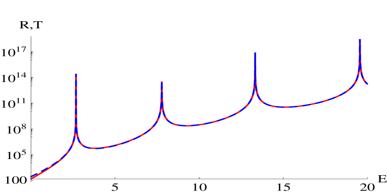
Figure 6: The poles in $R(E)$ (red/solid) and $T(E)$ (blue/dashed) at the bound state eigenvalues (see Fig. 3) of the open well, when we change $U_{0}\rightarrow-V_{0}$ in Eqs. (15,19). Here again we take $V_{0}=1$ and $a=1$.

Poles of reflection $r(k)=B/A$ and transmission $t(k)=C/A$ amplitudes, of the type $k=i\alpha$ ($\alpha=\sqrt{-E}$) are known to yield the discrete energy bound states of a potential well which converges to zero asymptotically (e.g. square well, Gaussian well). One may extend this idea to extract the bound state eigenvalues from the poles of $R(E)$ and $T(E)$. In a textbook [2], this has been done for the square well potential but unfortunately the negative energy poles of these coefficient have been shown as having $T=1$, whereas they should have been shown as much higher thin spikes representing $T=\infty$.

In Eq.(15), let us replace $U_{0}$ by $-V_{0}$, then $s\rightarrow iq$ and Hankel function $H^{(1)}_{ipa}(sa)$ converts to the modified Bessel function $K_{ipa}(qa)$ due to the property [20] that $H^{(1)}_{\nu}(iz)=-{2i}{\pi}e^{-\nu i\pi/2}K_{\nu}(z)$. In this way, the common denominator of $r(E)=B/A$ and $t(E)=C/A$ (15) yields the poles as

$$K_{ipa}(qa)~{}K^{\prime}_{ipa}(qa)=0,\quad p=\sqrt{2\mu(E+V_{0})}/\hbar$$ (22)

which is the combined bound state eigenvalue condition derived above (4,5) for the open potential well (1). Thus, if we plot $R(E)$ and $T(E)$ (15,19) by changing $U_{0}$ to $-V_{0}$ as in Fig. 5 for $V_{0}=1,a=1$, we get four poles in them at around $E\sim 2,7,13$ and 19, which are capable of yielding the correct bound state eigenvalues of the open well as mentioned in Fig. 2. It may be remarked that the thus changed expressions of $R(E)$ and $T(E)$ may not be of any use as the tunneling through open potential wells does not make any sense, however, these changed coefficients can yield the possible bound states of the well. Further, one may connect Eqs. (7) and (21) in this regard. When we change $U_{0}\rightarrow-V_{0}$ in (21), $s\rightarrow iq$, $G\rightarrow g$, $F\rightarrow f$ and $T_{WKB}(E)\rightarrow[1+e^{2if}]^{-1}$, one can readily get poles of $T_{WKB}(E)$ as $F=(n+1/2)\pi$ which is nothing but Eq. (7). We feel that such an interesting connection is often not discussed in textbooks.

VII Conclusion

Lastly, we hope that the new open well and the bottomless barrier constructed from the exponential potential will be welcome as solvable models which are rich in displaying several interesting quantum mechanical features through commonly available properties of Bessel and Hankel functions. Among the three (parabolic, triangular and exponential) analytically solvable bottomless barriers, the exponential barrier presented here has the new feature that the cross-over of the reflection and transmission probabilities can occur at the barrier-top and also either below a thicker barrier or above a thinner barrier. This is generally true for bounded potential barriers which vanish asymptotically on one or both sides. The simple WKB approximation does not yield this interesting result and the numerical integration of Schrödinger equation is not plausible due to the lack of generic asymptotic boundary conditions, it requires analytic solutions in every particular case.

References

References

- (1) Griffith D. J. 2011 Introduction to Quantum Mechanics edition (New-Delhi: Pearson)
- (2) Merzbacher E. 1970 Quantum Mechanics (John Wiley and Sons, Inc.: New York) edition
- (3) Landau L. D. and Lifshitz E. M. 1977 Quantum Mechanics (Pergamon Press, N.Y) edition.
- (4) Rapp D. 1971 Quantum Mechanics (Holt, Rinehart and Winston, Inc.: N.Y.)
- (5) Bates D. R. 1961 Quantum Theory (I Elements) (Academic Press: N.Y.) pp. 238-242.
- (6) Morse P. M. and Feshbach H. 1953 Methods of Theiretical Physics, Vol. 2 (McGraw-Hill Book Co. Inc.: N.Y) pp. 1651-1660.
- (7) Gendenshtein L. 1983 Zh. Eksp. Teor. Fiz. Pis. Red:38 299 (JETP Lett. 38 356)
- (8) Ginocchio J.N. 1984 Ann. Phys. 152 203.
- (9) Calogero F. and Degasperis A. 1982 Spectral Transform and Soliton I (North Holland, New-York) pp. 429-437.
- (10) Ahmed Z. 2006 Int. J. Mod. Phys. A 21 4439.
- (11) Ahmed Z. 1991 Phys. Lett. A 157 1.
- (12) Ahmed Z. 1993 Phys. Rev. A 1993 47 4761.
- (13) Ahmed Z. 1997 J. Phys. A: Math. Gen. 30 5243.
- (14) Dutt R., Khare A. and Sukhatme U.P. 1988 Am. J. Phys. 56 163.
- (15) Levai G. 1991 J. Phys. A: Math. Gen. 24 131.
- (16) Khare A. and Sukhatme U.P. 1988 J. Phys. A: Math. Gen. L501.
- (17) G. Levai, F. Cannata, A. Ventura 2001 J. Phys. A: Math. Gen. 34 839.
- (18) Ahmed Z. 2010 Am. J. Phys. 79 682.
- (19) D. ter Har 1964 Selected Problems in Quantum Mechanics ̵͑Academic, New York) see the solution to Problem 6, p. 360; V. I. Kogan and V. M. Galitskiy 1963 Problems in Quantum Mechanics (͑Prentice-Hall, Englewood Cliffs, NJ) pp. 334-337.
- (20) Abromowitz M., Stegun I.A 1970 Handbook of Mathematical Functions (Dover: New York) pp. 358-378.
- (21) Ahmed Z., Kumar S., Sharma M. and Sharma V. 2016 Eur. J. Phys. 37 045406.