Quantum cascade driving: Dissipatively mediated coherences

Abstract

Quantum cascaded systems offer the possibility to manipulate a target system with the quantum state of a source system. Here, we study in detail the differences between a direct quantum cascade and coherent/incoherent driving for the case of two coupled cavity-QED systems. We discuss qualitative differences between these excitations scenarios, which are particular strong for higher-order photon-photon correlations: $g^{(n)}(0)$ with $n>2$. Quantum cascaded systems show a behavior differing from the idealized cases of individual coherent/incoherent driving and allow to produce qualitatively different quantum statistics. Furthermore, the quantum cascaded driving exhibits an interesting mixture of quantum coherent and incoherent excitation dynamics. We develop a measure, where the two regimes intermix and quantify these differences via experimentally accessible higher-order photon correlations.

I Introduction

Quantum light sources are realized for many different material platforms in semiconductor, atom and molecular systems A.J.Shields (2007); Sim et al. (2012); Munoz et al. (2014); P.Lodahl et al. (2017); Strauf and Jahnke (2011) and offer an exciting testbed for nonlinear quantum dynamics Kabuss et al. (2011), including quantum ghost imaging, two-photon-spectroscopy Gonzalez-Tudela et al. (2013); Peiris et al. (2017); Dorfman et al. (2016) and quantum light spectroscopy M.Kira et al. (2011); Kira and Koch (2006a, b). Prototypical single photon emitters based on semiconductor nanostructures are produced I.Aharonovich et al. (2016); Gaisler (2009); Buckley et al. (2012) and used in quantum cryptography protocols H.J.Kimble (2008); Zoller et al. (2005); Jennewein et al. (2000) and quantum sensing Walmsley (2015). Recently, practical realization of intense and tunable thermal sources have become accessible Beach and Hartmann (1984); Strauß et al. (2016); Aßmann and Bayer (2011); Jahnke et al. (2016) and are applied experimentally for photon-statistics excitation spectroscopy Kazimierczuk et al. (2015); Strauß et al. (2016) and to read-out quantum beating of hyperfine levels via a modulation with pulse separation Beach and Hartmann (1984). Polarization-entangled photon sources, another class of quantum light sources, are electrically driven and triggered on demand A.J.Shields (2007). For highly- efficient and indistinguishable twin photon sources T.Heindel et al. (2017) this is possible as well in the context of N-photon bundle emitters Munoz et al. (2014) and on demand time-ordered photon pairs Müller et al. (2014) .

The rich variety of quantum light is accompanied by exciting proposals. Single photon excitation purifies non-classical states and suppresses fluctuations López Carreño et al. (2015) and allows for Hilbert-state addressing Carreño and Laussy (2016). Entangled photon pairs are proposed for ultrafast double-quantum-coherence spectroscopy of excitons with entangled photons Richter and Mukamel (2010) or quantum gates based on entanglement swapping protocols Troiani (2014). The Schmidt decomposition allows to analyze the material response function to obtain information about otherwise inaccessible resonances of a complex system Schlawin and Buchleitner (2015). This connects to the context of quantum optical spectroscopy Kira and Koch (2006a); Hall et al. (1989) and nonlinearity sensing via photon-statistics excitation spectroscopy Aßmann and Bayer (2011); Carmele et al. (2009).

A very convenient method to simulate quantum excitation experiments is the quantum cascade setup developed at the same time by Gardiner Gardiner (1993) and Carmichael Carmichael (1993). The quantum cascade approach allows a self-consistent mapping of the quantum excitation onto a second-system, via the quantum Langevin Gardiner (1993) or quantum stochastic Schrödinger equations Gardiner and Zoller (2000); Carmichael (2009). This mechanism is a dissipatively mediated excitation process as the output (measurement) of the source system is the input (excitation) of the target system. This excitation strategy differs strongly from a bath input (thermal equilibrium) or laser excitation, which adds coherence to the system. In contrast, the quantum cascaded driving allows a photon-statistical fine tuning in between these regimes and renders a transient regime accessible, where thermal statistics and quantum coherences coexist and intertwine via quantum emitters.

In this work, we theoretically discuss this intermixing and transition dynamics by employing a quantum cascaded system. In Sec. II, we derive the basic quantum cascaded coupling in the master equation formalism, equivalent to the method of Langevin operators Gardiner and Collett (1985); Carreño and Laussy (2016) and the quantum stochastic Schrödinger equation Carmichael (1993); Pichler and Zoller (2016). We apply this quantum cascaded coupling in Sec. III to a specific example: an incoherently pumped single quantum emitter in a cavity as the source and as the target one or two identical quantum emitters coupled to a cavity. We show that the intensity-intensity correlation $g^{(2)}(0)$ of the target system follows the intensity-intensity correlation of the source in the regime of interest, however, classically degraded due to the mediating bath. In Sec. IV, we show that the response of the target system follows not universally the output of the source system: Higher-order intensity correlations $g^{(n)}(0)$ exhibit a completely different picture. Via these higher-order correlations, we finally discuss the qualitatively different behavior of the cascaded setup in comparison to the typical excitation scenarios of coherent and incoherent pumping in Sec. V. In Sec VI, we conclude and summarize the findings.

II Quantum cascade model

To investigate the dynamics of a quantum cascaded system, we derive a master equation in the Born-Markov limit Carreño and Laussy (2016); Gardiner and Collett (1985); Collett and Gardiner (1984); *PhysRevLett.56.1917.

We will consider systems as depicted in Fig. 1 , i.e. a source quantum system with Hamiltonian $H_{s}$ coupled via a thermal bath, $H_{c}$ to target quantum system $H_{t}$. The full Hamiltonian reads: $H=H_{0}+H_{s}+H_{c}+H_{t}$, with $H_{0}$ including the free evolution dynamics of all quantities in the total system. At this point, we do not define $H_{s}$ and $H_{t}$, but focus on the coupling Hamiltonian $H_{c}$, which is given in a rotating frame in correspondence to $H_{0}$ and reads in the rotating wave approximation:

$$\frac{H_{\mathrm{c}}}{\hbar}=\int d\omega\ b(\omega)\Big{[}K^{s}_{\omega}J_{s}^{\dagger}(t)+K^{t}_{\omega}J^{\dagger}(t,\tau)\Big{]}+\text{H.c.},$$ (1)

where $\tau$ describes the finite time delay between the target and source system and $J_{s},J_{t}$ describe a single operator or a superposition in the source and target system, respectively. The coupling of the source/target system to the connecting reservoir is $K^{s/t}_{\omega}$, which we set independent of the frequency in the narrow bandwidth limit $K^{s/t}_{\omega}\equiv K^{s/t}_{0}$.

To derive the quantum cascaded couling, we employ the canonical derivation of the master equation in the Born-Markov limit with $\chi_{\mathrm{tot}}(t)=\rho(t)\rho_{B}(0)$, assuming the coupling reservoir in equilibrium and in a thermal state Breuer and Petruccione (2002); Carmichael (1999):

$$\frac{d\rho}{dt}|_{c}=-\frac{1}{\hbar^{2}}\int_{0}^{t}ds\mathrm{Tr}_{B}\left\{\left[H_{\mathrm{c}}(t),\left[H_{\mathrm{c}}(s),\rho(t)\rho_{B}\right]\right]\right\}.$$ (2)

We assume the thermal bath to be in the vacuum state and consider only contribution proportional to $\big{\langle}b(\omega)b^{\dagger}(\omega)\big{\rangle}$ and assume the commutator relations $[b(\omega),b^{\dagger}(\omega^{\prime})]=\delta(\omega-\omega^{\prime})$. Given these conditions, the double commutator can be evaluated, and we yield the following master equation after tracing out the bath degrees of freedom:

$$\frac{d\rho}{dt}|_{c} =-2\pi\sum_{i=s,t}(K^{i}_{0})^{2}\int_{0}^{t}ds\delta(s-t)$$

$$\times\left[J_{i}^{\dagger}(t)J_{i}^{\phantom{\dagger}}(s)\rho(s)-J^{\phantom{\dagger}}_{i}(t)\rho(s)J^{\dagger}_{i}(s)-J^{\phantom{\dagger}}_{i}(s)\rho(s)J^{\dagger}_{i}(s)+\rho(s)J_{i}^{\dagger}(s)J_{i}^{\phantom{\dagger}}(t)\right]$$

$$-2\pi K^{s}_{0}K^{t}_{0}\int_{0}^{t}ds\delta(s-(t-\tau))$$

$$\times\left[J_{t}^{\dagger}(t)J_{s}^{\phantom{\dagger}}(s)\rho(s)-J^{\phantom{\dagger}}_{t}(t)\rho(s)J^{\dagger}_{s}(s)-J^{\phantom{\dagger}}_{s}(s)\rho(s)J^{\dagger}_{t}(t)+\rho(s)J_{s}^{\dagger}(s)J_{t}^{\phantom{\dagger}}(t)\right]$$

$$-2\pi K^{s}_{0}K^{t}_{0}\int_{0}^{t}ds\delta(s-(t+\tau))$$

$$\times\left[J_{s}^{\dagger}(t)J_{t}^{\phantom{\dagger}}(s)\rho(s)-J^{\phantom{\dagger}}_{s}(t)\rho(s)J^{\dagger}_{t}(s)-J^{\phantom{\dagger}}_{t}(s)\rho(s)J^{\dagger}_{s}(s)+\rho(s)J_{t}^{\dagger}(s)J_{s}^{\phantom{\dagger}}(t)\right].$$ (3)

We take into account that $\int^{t}_{0}ds\delta(t-s)h(s)=h(t)/2$ and that $s\leq t$. By defining $K^{i}_{0}=\sqrt{\gamma_{i}/(2\pi)}$, where $\gamma_{i}$ are the decay rate of the subsystems that couple source and target. Then, one coupling contribution between target and source vanishes. The full master equation in the Born-Markov limit reads:

$$\frac{d\rho}{dt} =\frac{1}{i\hbar}[H_{s}+H_{t},\rho]$$

$$+\sum_{i=s,t}\frac{\gamma_{i}}{2}\left(2J^{\phantom{\dagger}}_{i}(t)\rho(t)J^{\dagger}_{i}(t)-\{J^{\dagger}_{i}(t)J^{\phantom{\dagger}}_{i}(t),\rho(t)\}\right)$$

$$-\sqrt{\gamma_{s}\gamma_{t}}\left(J_{t}^{\dagger}(t)J_{s}^{\phantom{\dagger}}(t_{D})\rho(t_{D})-J^{\phantom{\dagger}}_{t}(t)\rho(t_{D})J^{\dagger}_{s}(t_{D})\right)$$

$$-\sqrt{\gamma_{s}\gamma_{t}}\left(\rho(t_{D})J_{s}^{\dagger}(t_{D})J_{t}^{\phantom{\dagger}}(t)-J^{\phantom{\dagger}}_{s}(t_{D})\rho(t_{D})J^{\dagger}_{t}(t)\right),$$ (4)

with $t_{D}=t-\tau$. In our setup, the delay $\tau$ is small and can be set to zero safely within our Markovian approximation. Transforming back from the rotating frame, the full master equation reads:

$$\frac{d\rho}{dt} =\frac{1}{i\hbar}[H_{0}+H_{s}+H_{t},\rho]$$

$$+\sum_{i=s,t}\frac{\gamma_{i}}{2}\left(2J^{\phantom{\dagger}}_{i}\rho J^{\dagger}_{i}-\{J^{\dagger}_{i}J^{\phantom{\dagger}}_{i},\rho\}\right)$$

$$-\sqrt{\gamma_{s}\gamma_{t}}\left([J_{t}^{\dagger},J_{s}^{\phantom{\dagger}}\rho]+[\rho J^{\dagger}_{s},J^{\phantom{\dagger}}_{t}]\right).$$ (5)

Given this result, we can investigate different kinds of systems and study the particular features of a quantum cascaded driving. To characterize the cascaded driving, we choose first a specific system and then propose the photon-photon correlation functions as a measure for coherence in the system. We will see that the cascaded system(exhibits different regimes of excitation depending on the source excitation, however, the source state is not straight forwardly mapped to the target system) is remarkably much closer to a coherent driving setup, although it is of purely dissipative nature.

III Example: Coupled cQED - Systems

Figure 1: Schematic depiction of the studied setup. The source cavity, which contains a TLS, is pumped incoherently with rate $\Gamma^{P}_{s}$. The emission of the source cavity is fed into the one or two emitters contained in the target cavity.

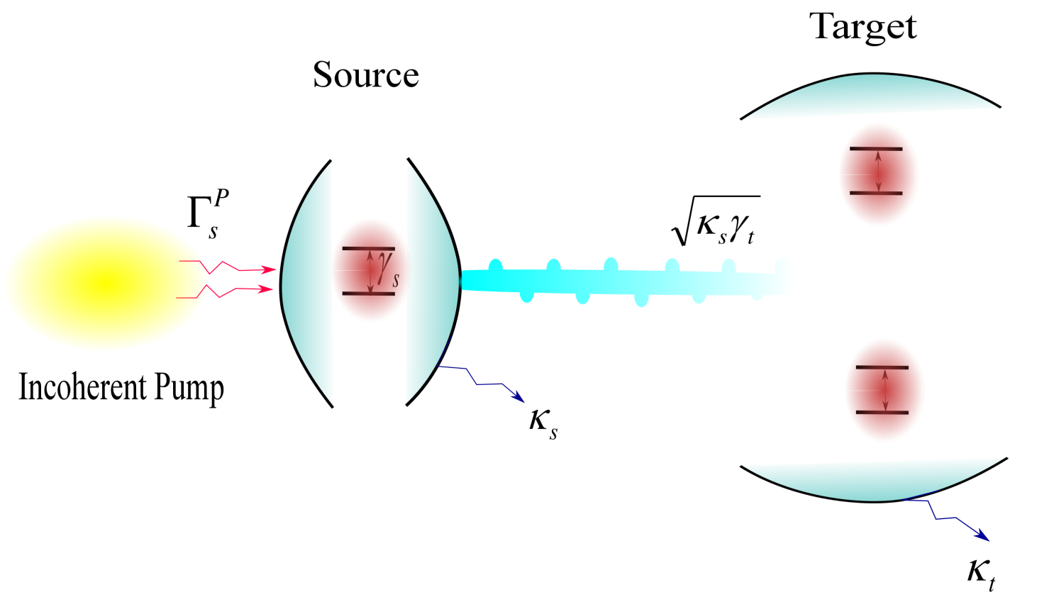
As a platform to investigate quantum excitation in comparison to coherent and incoherent driving, we focus on a coupled cavity quantum electrodynamics (cQED) system, Fig. 1. As a source system, we consider a single emitter coupled to a single cavity mode, which is the prototypical Jaynes-Cummings Hamiltonian:

$$H_{\mathrm{s}}=\hbar g_{s}\left(a_{s}^{\dagger}\sigma_{s}^{-}+\sigma_{s}^{+}a_{s}\right),$$ (6)

where $g_{s}=0.1\text{ps}^{-1}$ denotes the coupling element between the cavity field with creation(annihilation) operators $a^{(\dagger)}$ and the fermionic degrees of freedom, described via the spin Pauli matrices $\sigma_{s}^{(+/-)}$. The coupling operator from the source to the cavity is chosen to be $J_{s}:=a_{s}$. To control the source system, we assume an incoherent pumping mechanism. For far-off resonant driving, this pump mechanism can safely be described via Del Valle and Laussy (2010); *PhysRevA.84.053804

$$\mathcal{D}[\sqrt{\Gamma^{P}_{s}}\sigma^{+}_{s}]\rho:=\Gamma^{P}_{s}\left(2\sigma_{s}^{+}\rho\sigma_{s}^{-}-\{\sigma_{s}^{-}\sigma_{s}^{+},\rho\}\right),$$ (7)

assuming the transfer of excitation from the ground state to the excited state of the fermionic system, and the definition $\mathcal{D}[J]\rho:=2J\rho J^{\dagger}-\{J^{\dagger}J,\rho\}$. In the following, we will fix all parameters (cf. Tab. 1) but $\Gamma^{P}_{s}$, which is controllable via the intensity of the applied external pumping field, or even electrically steerable in semiconductor nanotechnology platforms A.J.Shields (2007); Stevenson et al. (2006); Yuan et al. (2002); Schulze et al. (2014).

parameter	value ($\mathrm{ps}^{-1}$)
$g_{s}$	0.1
$g_{t}$	0.1
$\gamma_{s}$	0.02
$\gamma_{t}$	0.5
$\kappa_{s}$	0.1
$\kappa_{t}$	0.005

Table 1: Parameters used for the cascaded setup throughout the manuscript.

The source is an incoherently pumped single emitter coupled to a single cavity mode. Depending on the pumping strength, the statistics of the output field can be tuned over a wide regime, starting for weak pumping in the single-photon, or antibunching regime $g^{(2)}(0)=\big{\langle}(a^{\dagger}_{s})^{2}(a^{\phantom{\dagger}}_{s})^{2}\big{\rangle}/\big{\langle}a^{\dagger}_{s}a^{\phantom{\dagger}}_{s}\big{\rangle}^{2}<1$ via a synchronized laser transition $g^{(2)}(0)\approx 1$ to the thermal state for a pumping parameter $\Gamma^{P}_{s}\gg g_{s}$. To complete the picture, we assume a radiative decay for the source via

$$\mathcal{D}[\sqrt{\gamma_{s}}\sigma_{s}^{-}]\rho:=\Gamma^{s}_{r}\left(2\sigma_{s}^{-}\rho\sigma_{s}^{+}-\{\sigma_{s}^{+}\sigma_{s}^{-},\rho\}\right).$$ (8)

The radiative decay amounts to $\Gamma^{s}_{r}=0.02\text{ps}^{-1}$. So, we assume not a perfect $\beta=1$ laser dynamics for the single emitter laser, as radiative decay is not fully absorbed by the cavity mode.

As a target system, we choose also the Jaynes-Cummings Hamiltonian but with two emitters:

$$H_{\mathrm{t}}=\hbar\sum_{j=1,2}g_{j,t}\left(a_{t}^{\dagger}\sigma_{j,t}^{-}+\sigma_{j,t}^{+}a_{t}\right),$$ (9)

where the emitter of the target system $\sigma_{j,t}^{-/+}$ couples to the single mode cavity with the strength of $g_{j,t}=g_{t}=0.1\text{ps}^{-1}$ and the emitters are identical. Here, the coupling operator from the target system is chosen to be $J_{i,t}:=\sigma^{-}_{i,t}$ $(i=1,2)$, i.e. the coupling to the source is individual and not in superposition. We assume an additional cavity loss for the target system via:

$$\mathcal{D}[\sqrt{\kappa_{t}}a_{t}^{\phantom{\dagger}}]\rho:=\kappa_{t}\left(2a^{\phantom{\dagger}}_{t}\rho a^{\dagger}_{t}-\{a^{\dagger}_{t}a^{\phantom{\dagger}}_{t},\rho\}\right)$$ (10)

and setting the photon life time $\kappa_{t}=0.005\text{ps}^{-1}$.

The free evolution is governed by $H_{0}$ and given as:

$$H_{0}=\hbar\omega_{0}\sum_{i=s,t}a_{i}^{\dagger}a^{\phantom{\dagger}}_{i}+\hbar\omega_{e}(\sigma_{s}^{+}\sigma_{s}^{-}+\sum_{i=1,2}\sigma_{t,i}^{+}\sigma_{t,i}^{-}),$$ (11)

We assume a resonant dynamics between cavity and the emitter $\omega_{e}=\omega_{0}$ and also in between the source and target. Therefore, the full master equation reads:

$$\frac{d\rho}{dt} =\frac{1}{i\hbar}[H_{0}+H_{s}+H_{t},\rho]$$

$$+\mathcal{D}[\sqrt{\Gamma^{P}_{s}}\sigma_{s}^{+}]\rho+\mathcal{D}[\sqrt{\gamma_{s}}\sigma_{s}^{-}]\rho+\mathcal{D}[\sqrt{\kappa_{s}}a^{\phantom{\dagger}}_{s}]\rho$$

$$+\mathcal{D}[\sqrt{\kappa_{t}}a^{\phantom{\dagger}}_{t}]\rho+\sum_{i=1,2}\mathcal{D}[\sqrt{\gamma_{t}}\sigma_{t,i}^{-}]\rho$$

$$-\sqrt{\kappa_{s}\gamma_{t}}\sum_{i=1,2}\left([\sigma^{+}_{t,i},a^{\phantom{\dagger}}_{s}\rho]+[\rho a^{\dagger}_{s},\sigma_{t,i}^{\phantom{\dagger}}]\right).$$ (12)

This master equation is numerically evaluated with a fourth-order Runge-Kutta algorithm for different values of $\Gamma^{P}_{s}$. We keep throughout the discussion all other values fixed and cast the master equation Eq. (III) into the basis $\langle e_{s},p_{s},e_{t},p_{t}|\rho|e_{s}^{\prime},p_{s}^{\prime},e_{t}^{\prime},p_{t}^{\prime}\rangle$ with $e_{i}$ emitter states and $p_{i}$ photon manifold of source and target $i=s,t$. We compute the observables for different photon manifold cut-offs $p_{i}<N_{i}$ until convergence is reached, i.e. the corresponding and discussed observable do not change by increasing the cut-off further. We restrict our discussion in the following to observables of photon manifolds $p_{i}\leq 10$.

Figure 2: Second order correlation functions $g^{(2)}(0)$ of source (red, solid) and one (blue, dashed dotted) and two (green, dashed) tLSs in the target cavity. For low pump rates the target, in contrast to the source, shows rather a bunching behavior. When increasing the pump strength,for both source and target, a transition to the thermal regime occurs.

We discuss the response of the target system with respect to the photon-statistics of the output field. The output is included via the cavity loss of the target, and can be measured in Hanbury Brown and Twiss setups via the second-order correlation function, defined in the steady state limit as Loudon (2000):

$$g^{(2)}_{\mathrm{stat}}(\tau)=\lim\limits_{t\rightarrow\infty}\frac{\left\langle a^{\dagger}_{i}(t)a^{\dagger}_{i}(t+\tau)a^{{\phantom{\dagger}}}_{i}(t+\tau)a^{{\phantom{\dagger}}}_{i}(t)\right\rangle}{\left\langle a^{\dagger}_{i}(t)a^{{\phantom{\dagger}}}_{i}(t)\right\rangle^{2}},$$ (13)

where for the source $i=s$ and for the target cavity $i=t$. We consider here only the coincidence rates for zero delay $\tau=0$, as in this limit quantum effects in the correlation are prominent.

In Fig. 2, we numerically evaluate the $g^{(2)}(0)$ for the source (red, solid) and target with one (blue, dashed dotted) and two (green, dashed) TLSs for different incoherent pumping strengths $\Gamma^{P}_{s}$:

The source can be driven into the antibunching regime $g^{(2)}<1$ for driving strengths of $\Gamma^{P}_{s}<g_{s}$, where single photons are emitted. The cavity coupling is not strong enough to produce more than one cavity photon, before the cavity loss and dissipation forces the photon to leave the resonator. The source dynamics stays antibunched for a wide range of parameters and turns coherent for a pumping strengths $\Gamma^{P}_{s}>g_{s}$ and for even larger pumping, the pumping induced dephasing adiabatically eliminates the emitter dynamics and the output field equilibrates into a thermal state Gartner (2011); Rice and Carmichael (1994); Ritter et al. (2010).

Focusing now on the target dynamics, we observe that the dissipative coupling via the reservoir leads to a more classical response for one (blue, dashed dotted) as well as two TLSs (green, dashed line). In comparison to the source statistics, even in the case of two quantum emitters, i.e., with a stronger quantum nonlinearity, the photon statistics in target cavity is less non-classical. We can explain this due to the dissipative transfer mechanism between the cavities, leading to thermal mixture and loss of coherence from the source to the target. We observe furthermore that in the regime $\Gamma^{P}_{s}>g_{s}$, the response follows the source dynamics, and we conclude that a quantum cascaded coupling does not qualitatively change the second-order photon correlation function of the target.

However, we will see that this is not the case for higher-order photon correlation functions, which we discuss in the next section.

IV Beyond the second order photon correlation

Figure 3: Correlation functions in the steady state, when the pump strength is equal to the cavity coupling ($\Gamma^{P}_{s}=g$) for source (red, solid) and target with two TLSs (green, dashed) and a single TLS (blue, dashed dotted). The solid, dashed and dash dotted gray lines present thermal, coherent and pure quantum light. The source is antibunched and in the subpoissonian regime for all orders in the correlation function. The target with a single TLS exhibits thermal light. However, the target cavity when containing two TLSs shows a transitional behavior, where it starts out in the sub-thermal regime but goes to the sub-Poissonian regime for higher orders.

Figure 4: Higher-order correlation functions of the source $g^{(n)}_{s}(0)$ and target system $g^{(n)}_{t}(0)$ for different incoherent pumping strength of the source system $\Gamma^{P}_{s}$. Remarkably, the target system exhibits a different behavior than the source system.

Experimentally, higher-order photon-correlations have become accessible Aßmann et al. (2009). They allow to characterize the quantum light field in photon detection experiments more precisely. For example, a $g^{(2)}(0)\approx 1$ is often taken to be a sign for a coherent light field (in the Glauber state), or a Fock state with a large photon number: $g^{(2)}_{\text{Fock}}(0)=1-1/N\rightarrow 1$ for $N=\big{\langle}a^{\dagger}a\big{\rangle}\gg 1$. However, only considering higher-order correlations allows for a definite characterization of the light field. These are defined for $\tau=0$ and in the steady-state as

$$g^{(n)}_{\mathrm{stat}}(0)=\frac{\left\langle a^{\dagger n}_{i}a^{{\phantom{\dagger}}n}_{i}\right\rangle}{\left\langle a^{\dagger}_{i}a^{{\phantom{\dagger}}}_{i}\right\rangle^{n}},$$ (14)

where $i=s$ for the source and $i=t$ for the target cavity. Measuring such higher-order correlations allows to discriminate output fields even in case, when the $g^{(2)}(0)$ function value is equal. For example, the Fock state higher-order correlation functions read $g^{(n)}_{\text{Fock}}(0)=N!/[N^{n}(N-n)!]$ for $n<N=\big{\langle}a^{\dagger}a\big{\rangle}$ and therefore $g^{(n)}_{\text{Fock}}(0)>g^{(n+1)}_{\text{Fock}}(0)$ in contrast to a coherent distribution, which holds $g^{(n)}_{\text{coh}}(0)=g^{(n+1)}_{\text{coh}}(0)=1$. For a thermal light field with $\bar{n}$ mean photon number, the unnormalized higher-order correlation functions read $\left\langle a^{\dagger n}a^{n}\right\rangle=n!(\bar{n})^{n}$ and are calculated from $p_{n}=(\bar{n})^{n}/(1+\bar{n})^{n+1}$. For the correlation function holds then $g^{(n)}_{\text{therm}}(0)<g^{(n+1)}_{\text{therm}}(0)=(n+1)!$. We take these three limiting cases, to visualize our quantum cascade driving setup.

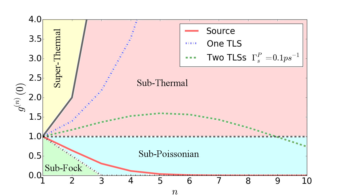
In Fig. 3, we plot the higher-order correlation functions for the source cavity (red, solid) and the target cavity with one (blue, dashed dotted) and two (green, dashed) TLSs. To illustrate regimes, we shaded the areas that distinguish between super-thermal and sub-thermal fields, and super- and sub-Fock states. The Fock state limits are taken, so that the number of Fock photons equals the order of the correlation function $N=n$. The correlations of the source $g^{(n)}_{s}(0)$ and target system $g^{(n)}_{t}(0)$ are shown for $\Gamma^{P}_{s}=0.1\text{ps}^{-1}=g$. The output field of the source shows a monotonic behavior, i.e. $g^{(n)}_{s}>g^{(m)}$ for all $n<m<10$. That is, comparing to the shaded area, very characteristic for a non-classical output field. For one TLS in the target cavity, we also see a monotonic behavior, but this time with $g^{(n)}_{s}<g^{(m)}$ for all $n<m<10$. In contrast, the output field of the target with two TLSs does not exhibit this kind of monotonous behavior, e.g. $g^{(2)}_{t}(0)<g^{(3)}_{t}$ but $g^{(2)}_{t}(0)>g^{(6)}_{t}$. Given this difference, it is clear, that the target dynamics is not a simple image of the source, the differences cannot only be traced back to dissipative degradation from the source-target transfer. In the following, we will focus on the case of two TLSs, as we find interesting photon probability distributions for this case, and also, since the target system with one emitter does not show non-monotonic behavior in the parameter regime, in which we are interested in. The quantum cascade coupling introduces an own, remarkable behavior and prevents a straightforward imprinting of the source statistics on the target quantum statistics, i.e. the $g^{(n)}_{t}(0)$ distribution.

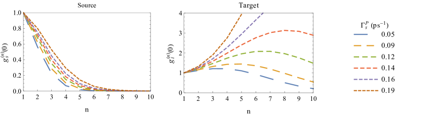
In Fig. 4, we investigate the higher-order correlation functions of the source $g^{(n)}_{s}(0)$ and target system $g^{(n)}_{t}(0)$ for different incoherent pumping strengths of the source system $\Gamma^{P}_{s}$. Interestingly, the response of the target differs strongly from the source quantum statistics. The source system shows a monotonic behavior for all pumping strengths: $g^{(n)}_{s}(0)>g^{(m)}_{s}(0)$ for all $n<m\leq 10$. Furthermore, the quantum statistics approaches lower values and reaches small values for high orders. This behavior is expected, since the incoherent driving and the cooperativity Walls and Milburn (2008) $C_{s}=g_{s}^{2}/(\Gamma_{R}\kappa_{s})$ limits the achievable photon manifold, i.e. there is always a cut-off $n_{c}$ with $p_{n_{c}}=0$ and therefore the importance of higher-order correlations decreases: $g^{(n)}_{s}(0)\rightarrow 0$ for $(n-n_{c})\rightarrow 0$.

In contrast, the target system reaches first a maximum for a certain $m$ with $g^{(m)}_{t}(0)\geq g^{(n)}_{t}(0)$ for all $n$. This maximum shifts, as expected, for higher pumping strength towards larger $m$, since the maximum number of photons also shifts to larger values. After the maximum, the $g_{t}^{(n)}(0)$ distribution follows the trend of the source system towards lower values. This behavior is stable for a wide range of pumping strengths. Due to the presence of a cut-off in the source photon manifold $n_{c}$, the target quantum distributions will also, eventually, tend to zero. However, the target system follows only for large $n$, the source quantum statistics, always after passing a maximum. This maximum, however, can shift to very large values, and in particular from a certain pumping strength on: $\Gamma^{P}_{s}=0.2\text{ps}^{-1}$ (blue, dashed line).

Figure 5: The transition observed in the system illustrated by the second order finite difference at the $g^{(2)}$-function. While the source correlations cross from an upwards to a downwards turning point, the target correlations exhibit the opposing behavior. The curves cross at the coupling strength $g=0.1\mathrm{ps}^{-1}$ common to source and target.

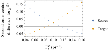
Furthermore, Fig. 4 shows a qualitative transition of the target system in the correlation functions. For low incoherent pump strengths, the curve is turning downwards. Then there is a transition towards the regime, where the curve turns upwards. We quantify this by the second order central difference defined as

$$g^{(n)\prime\prime}=\frac{g^{(n+1)}-2g^{(n)}+g^{(n-1)}}{(n+1-n)(n-(n-1))}.$$ (15)

During the transition from coherent to thermal behavior the $n$th order correlation function will flip successively up. Here, we characterize this transition by the second order difference at the $g^{(2)}$-function, which will first show the flip, so that the curve points here upwards. This is shown in Fig. 5, where we observe, that the target system goes from a downwards to an upwards turning point. At the same time the source system shows a transition from an upwards to a downwards turning point. The curves cross at the coupling strength $g=0.1\mathrm{ps}^{-1}$. Thus, even though it is not straightforwardly obvious how the source influences the target, we can illustrate the transition in the target system by a corresponding transition in the source system

To explain the origin of our results, in the next section, we compare the quantum statistics of the target system with a coherent and incoherent drive. We will see, that this maximum in the photon-correlation is not readily produced with either coherent or incoherent driving. Thus, the cascaded setup allows to create photon statistics not achievable with a reduced formulation.

V Properties of cascaded driving

Figure 6: Higher-order correlation functions of the target system with no quantum source pumping $\kappa_{t}=\Gamma^{P}_{s}=0$. Instead the target is directly pumped incoherently (left) and coherently (right) with $\Gamma^{P}_{t}=\sqrt{\gamma_{t}\kappa_{s}}$. Note the logarithmic scale for incoherent pumping, and the monotonous increase in contrast to the coherent driving induced maximum in the $g^{(n)}(0)$ distribution. The incoherent driving exhibits thermal statistics, while the coherent driving is close to coherent statistics for a wide range of pump parameters.

To characterize the quantum cascade, we compare the resulting higher-order correlation with a system that is coherently or incoherently driven. To model this situation, we switch the coupling between the source and target system off by setting $\kappa_{s}=0$. The driving of the target system is now included for the coherent driving by displacing the target’s photon operator according to $a^{\dagger}_{t}\rightarrow a^{\dagger}_{t}+\Gamma^{P}_{t}/g_{t}$ and for the incoherent driving case, we switch the operators of the incoherent pumping from $\mathcal{D}[\sqrt{\Gamma^{P}_{s}}\sigma^{+}_{s}]\rho\rightarrow\mathcal{D}[\sqrt{\Gamma^{P}_{t}}\sigma^{+}_{t}]\rho$.

Figure 7: Occupation probability of the Fock states for $\Gamma^{P}_{s}=0.1\mathrm{ps}^{-1}$ corresponding to the photon statistics shown in Fig. 3 (solid, blue). Due to the cascaded coupling the photon number distribution is exceptionally flat. This illustrates the photon statistics that deviate from the prototypical cases. For reference (dashed, orange), the coherent distribution is shown.

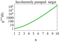
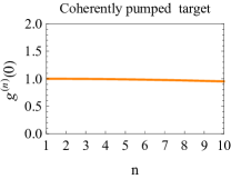
In Fig. 6, we compare the higher-order correlation functions for the case of coherent pumping (left panel) and incoherent pumping (right panel) of the target system. All parameter values are kept to allow comparison with the quantum cascaded case. Comparing the behavior of the correlation functions in the cascaded setup (cf. Fig. 4), with the incoherently and the coherently pump cases, we see a qualitatively different behavior. While, the cascaded setup exhibits a maximum in the correlation functions, the incoherently driven one exhibits thermal behavior, increasing monotonically and the coherently driven system exhibits close to coherent statistics. The form of the photon statistics for the cascaded system is distinctly different than for the other excitation scenarios. This is consistent with the findings in Ref. Carreño and Laussy (2016), where it is shown that, in principle, the target of a stationary cascaded system may access parts of the Hilbert space, that would not be accessible by other means. Here, we illustrate this finding by showing a physical system realizing this possibility.

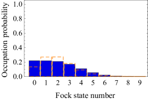
If we inspect the coupling terms, we can give some physical intuition for the observed result. While the cascaded coupling is derived using an intermediate bath and thus constitutes a dissipative coupling, the coupling preserves some properties of the source statistics in certain regimes. This becomes clear from the master equation Eq. (III). If one exchanges $\sqrt{\gamma_{t}\kappa_{s}}\rightarrow-\sqrt{\gamma_{t}\kappa_{s}}$, the system dynamics and results remain unchanged, as it is the same with $H_{t/s}\rightarrow-H_{t/s}$. This explains the part of the dynamics that preserve the source photon statistics for low pump strengths. This behavior is not expected from a dissipative coupling as the standard Lindblad form is independent of a change in the sign. For weak incoherent pumping, quantum coherences can be built up and those quantum processes are mediated via $a^{\dagger}_{s}$ to the coherences of the target system $\sigma^{+}_{t}$. In this limit, for high pumping strengths, the system becomes thermal. However, the intermediate coupling regime shows the transition, allowing for peculiar distributions by only partially imprinting the source photon statistics on the target in the high-order correlation functions. The Fock distribution corresponding to the statistics in Fig. 3 is shown in Fig. 7. Here, we observe a very flat distribution exhibiting a similar probability for the first few photon number states(solid,blue). This deviates from the coherent distribution(dashed,orange), which exhibits a maximum and the thermal distribution, which decreases monotonically. With this, we can explain the accessibility of new photon statistics by the mixture of Hamiltonian and decoherent coupling processes, mediated by the cascaded setup.

VI Conclusion

We investigated a quantum cascaded system, in which an incoherently pumped source system drives a target system with its quantum output field. As observables, we focused on higher-order photon- correlations $g^{(n)}(0)$. We find that the response of the target system differs strongly for different values of the incoherent pump parameter. For low values in comparison to the coupling constant of the target system $\Gamma^{P}_{s}<g_{t}$, the quantum statistics of the source system are imprinted on the target system. For larger values the target system’s output field resembles an incoherently driven quantum system. However, in an intermediate regime, a mixture of coherent and incoherent processes due to the coupling mechanism occurs leading to quantum statistics differing from the prototypical coherent and thermal shapes and giving rise to the possibility of producing flat photon distributions.