Base Station Selection for Massive MIMO Networks with Two-stage Precoding

Abstract

The two-stage precoding has been proposed to reduce the overhead of both the channel training and the channel state information (CSI) feedback for the massive multiple-input multiple-output (MIMO) system. But the overlap of the angle-spreading-ranges (ASR) for different user clusters may seriously degrade the performance of the two-stage precoding. In this letter, we propose one ASR overlap mitigating scheme through the base station (BS) selection. Firstly, the BS selection is formulated as a sum signal-to-interference-plus-noise ratio (SINR) maximization problem. Then, the problem is solved by a low-complex algorithm through maximizing signal-to-leakage-plus-noise ratio (SLNR). In addition, we propose one low-overhead algorithm with the lower bound on the average SLNR as the objective function. Finally, we demonstrate the efficacy of the proposed schemes through the numerical simulations.

I Introduction

The massive multiple-input multiple-output (MIMO) system has been considered as a promising technology to meet the capacity demand in the next generation wireless cellular networks [1]. In the frequency-division duplex (FDD) system where the uplink-downlink reciprocity does not exist, the CSI at the BS side should be obtained through the downlink training and the CSI feedback, which will lead to the unacceptable overheads [2]. To overcome this bottleneck, the joint spatial-division and multiplexing (JSDM) was recently proposed as one two-stage precoding scheme[3].

Several researchers followed the two-stage precoding and developed different prebeamforming methods[3, 4, 5, 6]. In [3], Adhikary et al. proposed one block diagonalization (BD) algorithm, whose main idea is projecting the channel eigenspace of the desired cluster into that for all the other clusters. In [4], an iterative prebeamforming algorithm was designed to maximize the signal-to-leakage-plus-noise ratio (SLNR). In [5], Chen and Lau developed a low-complex online iterative algorithm to track the prebeamformer. In [6], Sun et al. proposed the beam division multiplex access (BDMA) scheme to complete the optimal downlink transmission with only statistical CSI.

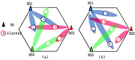
Figure 1: An downlink massive MIMO network with $L$ BSs, where clusters are randomly distributed. (a) One BS selection solution with serious ASR overlap. (b) Another BS selection solution with slight ASR overlap.

As mentioned in [3, 4, 5, 6], when the angle-spreading-ranges (ASRs) of the scattering rays for different clusters do not overlap, the orthogonal transmission can be achieved with the two-stage precoding. However, in practice, the ASRs for some clusters may overlap, which would degrade the performance of the two-stage precoding, especially in the high dense coverage scenario. Furthermore, the authors in [3, 4, 5, 6] only examined the single BS scenario and scheduled the clusters without (or with slight) ASR for transmission. In this letter, we consider one typical multiple BSs coverage scenario as shown in Figure 1, where three BSs with sector antennas of 120 degrees opening are equipped at the cell corners [7]. In such scenario, the two user clusters with serious ASR overlap at one BS may have no or slight ASR overlap at the others. For example, as shown in Figure 1, the clusters 2 and 4 have serious ASR overlap seen from BS1, but have no overlap when they are connected to BS2 or BS3. Hence, the serious ASR overlap may be mitigated through the BS selection, which can be formulated as a combinational optimization targeting at maximizing the sum SINR for all users. In [8], the authors prove that if the BS selection problems are considered together with the power control, then the optimal solution can be obtained. However, when the power is fixed, the optimal problem is NP-hard. To solve the optimization problem with low complexity, we develop one SLNR-based BS selection algorithm. It is proved that the proposed low complexity algorithm can achieve the optimal BS selection solution with the first category prebeamformers. Furthermore, we develop one low-overhead suboptimal algorithm, whose objective function is the lower bound of the average SLNR. Finally, numerical simulations are presented to validate the proposed algorithms.

II System Model and Preliminaries

II-A System Configuration and Channel Model

As shown in Figure 1, we consider a downlink massive MIMO network with $L$ BSs, where each BS employs an uniform linear array (ULA) with $N\gg 1$ antennas. It is assumed that the $K$ single-antenna users can be partitioned into $C$ clusters, where the users in the same cluster are almost co-located. We denote the set of all clusters as $\mathcal{C}=\{1,2,\cdots,C\}$. As a result, the number $K_{c}$ of the users in the cluster $c$ satisfies $\sum\limits_{c=1}^{C}K_{c}=K$. The $1\times N$ downlink channel vector from the BS $l$ to the user $k$ in the cluster $c$ is $\{\mathbf{h}_{c,k}^{l}\}^{T}$ and is assumed as block fading. We further define the $K_{c}\times N$ downlink channel matrix between the BS $l$ and the cluster $c$ as $\mathbf{H}_{c}^{l}=[\mathbf{h}_{c,1}^{l},\mathbf{h}_{c,2}^{l},,\cdots,\mathbf{h}_{c,{K_{c}}}^{l}]^{T}$.

Similar to the works [3, 5, 4, 6], the classical “one-ring” model [9] is applied to describe the channels. It can be readily checked that all the users in the same cluster share the same one-ring model parameters, which means that the users in the same cluster have the same $N\times N$ channel covariance matrix $\mathbf{R}_{c}^{l}$ at BS $l$, i.e., $\mathbb{E}\Big{\{}\mathbf{h}_{c,k}^{l}\big{[}{\mathbf{h}_{c,k}^{l}}\big{]}^{H}\Big{\}}=\mathbf{R}_{c}^{l},k=1,2,\cdots K_{c}.$ Furthermore, we can express $\mathbf{R}_{c}^{l}$ as

$$\left[\mathbf{R}_{c}^{l}\right]_{p,q}=\frac{1}{2\Delta_{c}^{l}}\int_{\theta_{c}^{l}-\Delta_{c}^{l}}^{\theta_{c}^{l}+\Delta_{c}^{l}}e^{\frac{-2i\pi(p-q)\sin(\alpha)\tau}{\lambda}}d\alpha,$$ (1)

where $\theta_{c}^{l}$ is the azimuth angle of the scatters ring, $[\theta_{c}^{l}-\Delta_{c}^{l},\theta_{c}^{l}+\Delta_{c}^{l}]$ is the ASR of the cluster $c$ at the BS $l$, $\tau$ is the antenna element spacing, and $\lambda$ is the carrier wavelength.

With eigen-decomposition, we have $\mathbf{R}_{c}^{l}=\mathbf{E}_{c}^{l}{\bm{{\Lambda}}_{c}^{l}}\big{[}\mathbf{E}_{c}^{l}\big{]}^{H}$, where the diagonal matrix ${\bm{{\Lambda}}_{c}^{l}}$ is the nonzero eigenvalue matrix, ${\mathbf{{E}}_{c}^{l}}$ contains the eigenvectors corresponding to the nonzero eigenvalues, and the rank of $\mathbf{R}_{c}^{l}$, i.e., $r_{c}^{l}$, is much smaller than $N$. Resorting to the Karhunen-Loeve representation, we can write the channel vector $\mathbf{h}_{c,k}^{l}$ as [3]

$$\mathbf{h}_{c,k}^{l}={\mathbf{E}_{c}^{l}}{\left\{\bm{{\Lambda}}_{c}^{l}\right\}}^{\frac{1}{2}}\mathbf{w}_{c,k}^{l},$$ (2)

where the entries of the $r_{c}^{l}\!\times\!\!1\!\!$ vector $\mathbf{w}_{c,k}^{l}\!$ are i.i.d. complex Gaussian distributed with zero mean and unit variance.

Let us represent the cluster set accessed to the BS $l$ as $\mathcal{C}_{l}$, which satisfies $\cup_{l=1}^{L}\mathcal{C}_{l}=\mathcal{C}$. Then, the received signal at the cluster $c$ accessed to the BS $l$ is

$$\mathbf{y}_{c\in\mathcal{C}_{l}}= \mathbf{H}_{c}^{l}\mathbf{P}_{c}^{l}\mathbf{d}_{c}^{l}+\sum_{c^{\prime}\in\mathcal{C}_{l},c^{\prime}\neq c}\mathbf{H}_{c}^{l}\mathbf{P}_{c^{\prime}}^{l}\mathbf{d}_{c^{\prime}}^{l}$$

$$~{}~{}~{}~{}~{}~{}~{}~{}~{}~{}~{}+\sum_{l^{\prime}\neq l}^{L}~{}\sum_{c^{\prime}\in\mathcal{C}_{l^{\prime}}}\mathbf{H}_{c}^{l^{\prime}}\mathbf{P}_{c^{\prime}}^{l^{\prime}}\mathbf{d}_{c^{\prime}}^{l^{\prime}}+\mathbf{n}_{c},$$ (3)

where $\mathbf{P}_{c}^{l}$ is the $N\times S_{c}$ precoding matrix for the cluster $c$ at the BS $l$, $\mathbf{d}_{c}^{l}$ with $\mathbb{E}\{\mathbf{d}_{c}^{l}(\mathbf{d}_{c}^{l})^{H}\}=\mathbf{I}$ is the $S_{c}^{l}\times 1$ data vector from BS $l$ to the cluster $c$, and the $K_{c}\times 1$ vector $\mathbf{n}_{c}\!\sim\!\mathcal{CN}(\mathbf{0},\sigma_{n}^{2}\mathbf{I}_{K_{c}})$ denotes the additive white Gaussian noise.

II-B Two-stage Precoding

As in [3, 5, 4, 6], the two-stage precoding can be written as

$$\mathbf{P}_{c}^{l}=\mathbf{B}_{c}^{l}\mathbf{V}_{c}^{l},$$ (4)

where the $N\times M_{c}^{l}$ prebeamforming matrix $\mathbf{B}_{c}^{l}$ only depends on the channel covariance matrices, and is used to eliminate the inter-cluster interferences; the $M_{c}^{l}\times S_{c}^{l}$ inner precoder $\mathbf{V}_{c}^{l}=[\mathbf{v}_{c,1}^{l},\mathbf{v}_{c,2}^{l},\cdots,\mathbf{v}_{c,K_{c}}^{l}]$, dealing with the intra-cluster interferences, can be designed with the $K_{c}\times M_{c}^{l}$ equivalent channel matrix $\overline{\mathbf{H}}_{c}^{l}={\mathbf{H}}_{c}^{l}\mathbf{B}_{c}^{l}$; $M_{c}^{l}$ is the dimension of $\overline{\mathbf{H}}_{c}^{l}$ seen by the inner precoder, and satisfies $S^{l}_{c}\leq M_{c}^{l}\leq r_{c}^{l}$. It can be found that $\overline{\mathbf{H}}_{c}^{l}$ possesses a much smaller number of unknown parameters than the original channel matrix $\mathbf{H}_{c}^{l}$.

The prebeamforming matrix designing methods can be divided into two categories according to the fact whether the inter-cluster interference is completely eliminated:

II-B1 The first category of the prebeamformers

the inter-cluster interference is eliminated completely by designing $\mathbf{B}_{c}^{l}$ to satisfy the following constraint,

$$(\mathbf{E}_{c^{\prime}}^{l})^{H}\mathbf{B}_{c}^{l}=0,\forall c^{\prime}\neq c.$$ (5)

The BD method in [3], BDMA method in [6], and DFT-based method in [10] fall into this category.

II-B2 The second category of the prebeamformers

the inter-cluster interference is not completely eliminated, which can be expressed mathematically as

$$(\mathbf{E}_{c^{\prime}}^{l})^{H}\mathbf{B}_{c}^{l}\approx 0,\forall c^{\prime}\neq c.$$ (6)

The approximate BD method in [3] and methods in [4] and [5] belong to this category.

III Proposed User Scheduling Scheme

III-A Problem Formulation

With prebeamforming, the inter-cluster interference is completely (or almost) eliminated. Without loss of generality, we assume that the intra-cluster interference is completely eliminated by the zero-forcing inner precoder $\mathbf{V}_{c}^{l}$. Then, the SINR of the user $k$ in the cluster $c\in\mathcal{C}_{l}$ can be derived from (II-A) as follow,

$$\text{SINR}_{c,k}^{l}=\frac{|(\mathbf{h}_{c,k}^{l})^{T}\mathbf{B}_{c}^{l}\mathbf{v}_{c,k}^{l}|^{2}}{\gamma_{c,k}^{l}+\sigma_{n}^{2}},$$ (7)

where

$$\gamma_{c,k}^{l}= \sum_{c^{\prime}\in\mathcal{C}_{l},c^{\prime}\neq c}~{}\sum_{k^{\prime}=1}^{K_{c^{\prime}}}|(\mathbf{h}_{c,k}^{l})^{T}\mathbf{B}_{c^{\prime}}^{l}\mathbf{v}_{c^{\prime},k^{\prime}}^{l}|^{2}$$

$$+\sum_{l^{\prime}=1,l^{\prime}\neq l}^{L}~{}\sum_{c^{\prime}\in\mathcal{C}_{l}}~{}\sum_{k^{\prime}=1}^{K_{c^{\prime}}}|(\mathbf{h}_{c,k}^{l^{\prime}})^{T}\mathbf{B}_{c^{\prime}}^{l^{\prime}}\mathbf{v}_{c^{\prime},k^{\prime}}^{l^{\prime}}|^{2}$$ (8)

is the power of the inter-cluster interference. Specifically, we get $\gamma_{c,k}^{l}=0$, if the first category prebeamforming is applied. Different from the classical user scheduling schemes [3, 4, 5, 6], we mitigate the inter-cluster interference through BS selection for each user cluster. For clear illustration, we present two examples in Fig. 1. With respect to one specific clusters distribution scenario, the BS selection scheme in Fig. 1-b suffers slighter ASR overlap than that in Fig. 1-a. Given $C$ clusters and $L$ BSs, the total number of the BS selection strategies is $L^{C}$. Since the ASR overlap decreases the desired signal power and increases the inter-cluster interference power, our task is to find the best strategy from all the possible ones to maximize the sum SINR, and the corresponding optimization problem can be formulated as

$$(\text{P}1)~{}~{}~{} \max_{\mathcal{C}_{1},\mathcal{C}_{l},\cdots,\mathcal{C}_{L}}\sum_{l=1}^{L}\sum_{c\in\mathcal{C}_{l}}\sum_{k=1}^{K_{c}}\text{SINR}_{c,k}^{l}$$ (9)

$$~{}~{}~{}~{}~{}\text{s.t.}~{}~{}\cup_{l=1}^{L}\mathcal{C}_{l}=\mathcal{C}.$$

The optimal problem (P1) is NP-hard, since the SINR of one specific cluster is closely related to the other user clusters’ BS selection strategy. Theoretically, it can be solved by the exhaustive search with the complexity $\mathcal{O}(L^{C})$, which is unacceptable for large $C$ and $L$. To reduce the complexity, we adopt SLNR as another optimization criterion.

III-B SLNR-Based BS Selection Algorithm with Low Complexity

The SLNR is defined as the ratio between the signal power to the desired receiver and total interference power to the undesired receivers, which is commonly used if the maximizing SINR problem is difficult to solve. The SLNR of the user $k$ in the cluster $c$ can be written as

$$\text{SLNR}_{c,k}^{l}= \frac{|(\mathbf{h}_{c,k}^{l})^{T}\mathbf{B}_{c}^{l}\mathbf{v}_{c,k}^{l}|^{2}}{\zeta_{c,k}^{l}+\sigma_{n}^{2}},$$ (10)

$$\text{where~{}~{}~{}~{}~{}~{}~{}~{}~{}~{} }\zeta_{c,k}^{l}= \sum_{c^{\prime}\in\mathcal{C},c^{\prime}\neq c}~{}\sum_{k^{\prime}=1}^{K_{c^{\prime}}}|(\mathbf{h}_{c^{\prime},k^{\prime}}^{l})^{T}\mathbf{B}_{c}^{l}\mathbf{v}_{c,k}^{l}|^{2}~{}~{}~{}~{}~{}~{}~{}~{}~{}~{}~{}~{}~{}~{}~{}~{}$$

is the leaked interference power. Specifically, $\zeta_{c,k}^{l}=0$, for the first category prebeamforming. Then, the BS selection problem can be reformulated as

$$(\text{P}2)~{}~{}~{} \max_{\mathcal{C}_{1},\mathcal{C}_{l},\cdots,\mathcal{C}_{L}}\sum_{l=1}^{L}\sum_{c\in\mathcal{C}_{l}}\sum_{k=1}^{K_{c}}\text{SLNR}_{c,k}^{l}$$ (11)

$$~{}~{}~{}~{}~{}\text{s.t.}~{}~{}\cup_{l=1}^{L}\mathcal{C}_{l}=\mathcal{C}.$$

The main difference between (P1) and (P2) can be summarized as follows: the SINR of one specific user depends on all other clusters’ BS selection strategies, while the SLNR is only related to its own selection decision. Thus, to achieve the optimal solution of (P2), we can separately implement the BS selection operation of each user cluster to maximize its own sum-SLNR, which is presented in Algorithm 1.

Theorem 1

When the prebeamforming methods in the first category is used, the SLNR-based BS selection algorithm achieves the optimal solution for the SINR maximization problem (P1).

Proof:

If the first category methods is applied, both $\gamma^{l}_{c,k}$ and $\zeta^{l}_{c,k}$ are zero. Therefore, the SLNR of a user is same with its SINR, which indicates that the problems (P2) and (P1) are equivalent and have the same optimal solution. ∎

In Algorithm 1, one cluster is assigned to a BS in the steps (4–7) of each iteration. Therefore, only $C$ iterations are required to complete BS selection for all $C$ clusters. Since only one BS is selected from $L$ ones in each iteration, the complexity of the Algorithm 1 is $\mathcal{O}(LC)$, which is much smaller than that of the exhaustive search. Take $C=25,L=3$ as a example, $\frac{LC}{L^{C}}=8.85\times 10^{-11}$.

Algorithm 1 SLNR-Based BS Selection Algorithm

0:   $\{(\mathbf{h}_{c,k}^{l})^{H}\mathbf{B}_{c}^{l}\}$,$\{\mathbf{V}_{c}^{l}\}$ .

0:  The clusters set that select each BS : $\mathcal{C}_{1},\mathcal{C}_{2},\cdots,\mathcal{C}_{L}$.

1:   Initialization:

2:   $\mathcal{C}_{l}=\emptyset,~{}\forall l=1,2,\cdots,L.$

3:  $c=1$.

4:  repeat

5:     $l^{*}_{c}=\arg\max_{l}\sum_{k=1}^{K_{c}}\text{SLNR}^{l}_{c,k}$, $\mathcal{C}_{l^{*}_{c}}=\mathcal{C}_{l^{*}_{c}}\cup\{c\}$.

6:      $c=c+1$.

7:  until $c>C$

8:  return  $\mathcal{C}_{1},\mathcal{C}_{2},\cdots,\mathcal{C}_{L}$.

III-C LASLNR-Based BS Selection Algorithm with Low Overhead

The previous subsection presents a low-complex BS selection algorithm. However, it requires the instant CSI of the equivalent effective channels between all the users and the BSs. Acquiring such a large amount of the equivalent channels would consume too much channel bandwidth. Therefore, we intend to give a low overhead BS selection method based on the average SLNR, which would only need the prebeamforming matrices $\{\mathbf{B}_{c}^{l}\}$ and channel covariance matrices $\{\mathbf{R}_{c}^{l}\}$. Unfortunately, it is very difficult to derive the closed-form expressions for the average SLNR. Thus, we derive a close-form lower bound on the average SLNR (LASLNR) as follows:

$$\mathbb{E}\{\text{SLNR}_{c,k}^{l}\}$$

$$\stackrel{{\scriptstyle(a)}}{{\geq}}\mathbb{E}\Bigg{\{}\frac{|(\mathbf{h}_{c,k}^{l})^{T}\mathbf{B}_{c}^{l}\mathbf{v}_{c,k}^{l}|^{2}}{P_{t}\sum_{c^{\prime}\in\mathcal{C},c^{\prime}\neq c}~{}\sum_{k^{\prime}=1}^{K_{c^{\prime}}}\|(\mathbf{h}_{c^{\prime},k^{\prime}}^{l})^{T}\mathbf{B}_{c}^{l}\|^{2}+\sigma_{n}^{2}}\Bigg{\}}$$

$$\stackrel{{\scriptstyle(b)}}{{\geq}}\frac{\mathbb{E}\big{\{}|(\mathbf{h}_{c,k}^{l})^{T}\mathbf{B}_{c}^{l}\mathbf{v}_{c,k}^{l}|^{2}\big{\}}}{\mathbb{E}\Big{\{}P_{t}\sum_{c^{\prime}\in\mathcal{C},c^{\prime}\neq c}~{}\sum_{k^{\prime}=1}^{K_{c^{\prime}}}\|(\mathbf{h}_{c^{\prime},k^{\prime}}^{l})^{T}\mathbf{B}_{c}^{l}\|^{2}+\sigma_{n}^{2}\Big{\}}}$$

$$\stackrel{{\scriptstyle(c)}}{{\geq}}\frac{\text{tr}\Big{\{}(\mathbf{B}_{c}^{l})^{H}\mathbf{R}_{c}^{l}\mathbf{B}_{c}^{l}\!\Big{\}}\!\!-\!\!(K_{c}-1)\lambda_{c}^{l}}{\sum_{c^{\prime}\in\mathcal{C},c^{\prime}\neq c}~{}\sum_{k^{\prime}=1}^{K_{c^{\prime}}}\text{tr}\Big{(}(\mathbf{B}_{c}^{l})^{H}\mathbf{R}_{c^{\prime}}^{l}\mathbf{B}_{c}^{l}\Big{)}+\sigma_{n}^{2}/P_{t}}$$

$$=\text{LASLNR}_{c,k}^{l},$$ (12)

where $\lambda_{c}^{l}$ is the largest eigenvalue of $\mathbf{R}^{l}_{c}$ and $P_{t}=\|\mathbf{v}_{c,k}^{l}\|^{2}$ is the transmitting power for each user. The derivation of (a) utilizes the matrix property equations $\|\mathbf{A}\mathbf{B}\|\leq\|\mathbf{A}\|\|\mathbf{B}\|$ and $\|\mathbf{v}^{l}_{c,k}\|=P_{t}$; (b) results from Jensen s inequality and the fact that $\mathbf{h}_{c,k}^{l}$ and $\mathbf{h}_{c^{\prime},k^{\prime}}^{l}$ are independent; (c) follows from Theorem 1 of [4].

Through replacing the step 4 in Algorithm 1 with

$$l^{*}_{c} =\arg\max_{l}\sum_{k=1}^{K_{c}}\text{LASLNR}^{l}_{c,k},$$ (13)

we can get the LASLNR-based low-overhead BS selection algorithm.

IV Numerical Results

In this section, we evaluate the performance of our proposed algorithms through numerical simulations. A typical single-cell with radius 1km is considered, where $L=3$ BSs are equipped at three cell corners. Each BS is equipped with a ULA of $N=128$ antennas. The number of the users in each cluster is set as 3. $C$ clusters are uniformly randomly distributed in the cell. The carrier frequency is $2$GHz. The massive MIMO channel is generated by (1) and (2). The variance of the noise is $\sigma_{n}^{2}=1$. The BD and the approximated BD (ABD) methods in [3] are used as the representatives for the first and second categories of the prebeamforming methods, respectively.

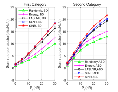
Figure 2: Sum-rate per cluster versus $P_{t}$ with $C=8,L=3$.

Figure 2 presents the curves of the sum-rate per cluster versus $P_{t}$, where the first and second categories of the prebeamforming methods are used, respectively. The proposed SLNR-based and LASLNR-based suboptimal algorithms are compared with the following methods: the exhaustive search for (P1), the scheme based on the largest energy of the channel coefficient matrix, and the random BS selection scheme. As observed from both figures, the proposed algorithms significantly outperform the randomly BS selection scheme and and the largest energy scheme. The LASLNR-based suboptimal algorithm almost achieves the same performance as the SLNR-based one. As mentioned in Theorem 1, the SLNR-based algorithm achieves the optimal solution for (P1) when the first category prebeamforming method is used, which is validated in Figure 2. Moreover, it is shown in Figure 2 that when the second category prebeamforming method is used the performance gap between SLNR-based algorithm and the optimal solution is also small.

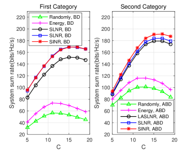
Figure 3: System sum-rate versus $C$ with $P_{t}$ = 20dB and $L=3$.

In Figure3 the impact of the number of clusters $C$ on the system sum-rate is demonstrated, where the first and second categories prebeamforming methods are used respectively. As we can see from the both figures, with the increase of $C$, the system sum-rate of all solutions increase at first and then decrease. The reason behind this is when $C$ is small, the ASR overlap is slight. Under this scenario, increasing $C$ will result in more served users and higher system sum-rate. As $C$ continues to increase, the cell becomes crowded and the ASR overlap becomes serious, which will degrade the system sum-rate. We can also see that the performance gaps between the proposed algorithms and the randomly selection solution become larger as $C$ increases. These observations indicate that the proposed scheme is effective to mitigate the ASR overlap, especially when the network is crowded.

V Conclusions

In this letter, we have proposed a BS selection scheme to mitigate ASR overlap for massive MIMO system with two-stage precoding. The BS selection problem was formulated as a combinatorial optimization problem targeting at maximizing the sum SINR. Then, we transformed the problem into a SLNR maximization optimization, which has low computational complexity. In order to further reduce the signaling overhead of SLNR maximization problem, a suboptimal solution was obtained by using the LASLNR as the objective function. The simulation results demonstrated that the proposed algorithms significantly improve the sum rate performance and the LASLNR-based algorithm achieves almost the same performance as the SLNR-based algorithm.

References

• [1] F.Β Rusek, D.Β Persson, B.Β K. Lau, E.Β G. Larsson, T.Β L. Marzetta, O.Β Edfors, and F.Β Tufvesson, β€œScaling up MIMO: Opportunities and challenges with very large arrays,” IEEE Signal Process. Mag., vol.Β 30, no.Β 1, pp. 40–60, Jan. 2013.
• [2] S.Β Noh, M.Β D. Zoltowski, and D.Β J. Love, β€œTraining sequence design for feedback assisted hybrid beamforming in massive MIMO systems,” IEEE Trans. Commun., vol.Β 64, no.Β 1, pp. 187–200, Jan. 2016.
• [3] A.Β Adhikary, J.Β Nam, J.-Y. Ahn, and G.Β Caire, β€œJoint spatial division and multiplexing the large-scale array regime,” IEEE Trans. Inf. Theory, vol.Β 59, no.Β 10, pp. 6441–6463, Oct. 2013.
• [4] D.Β Kim, G.Β Lee, and Y.Β Sung, β€œTwo-stage beamformer design for massive MIMO downlink by trace quotient formulation,” IEEE Trans. Commun., vol.Β 63, no.Β 6, pp. 2200–2211, Jun. 2015.
• [5] J.Β Chen and V.Β K.Β N. Lau, β€œTwo-tier precoding for FDD multi-cell massive MIMO time-varying interference networks,” IEEE J. Sel. Areas Commun., vol.Β 32, no.Β 6, pp. 1230–1238, Jun. 2014.
• [6] C.Β Sun, X.Β Gao, S.Β Jin, M.Β Matthaiou, Z.Β Ding, and C.Β Xiao, β€œBeam division multiple access transmission for massive MIMO communications,” IEEE Trans. Commun., vol.Β 63, no.Β 6, pp. 2170–2184, Jun. 2015.
• [7] Scanferla, D., β€œStudies on 6-sector-site deployment in downlink LTE”, Eindhoven University of Technology, Jan. 2012.
• [8] T. Van Chien, E. BjΓΆrnson and E. G. Larsson, β€œJoint power allocation and user association optimization for massive MIMO Systems,” IEEE Trans. Wireless Commun., vol. 15, no. 9, pp. 6384-6399, September 2016.
• [9] A.Β Abdi and M.Β Kaveh, β€œA space-time correlation model for multielement antenna systems in mobile fading channels,” IEEE J. Sel. Areas Commun., vol.Β 20, no.Β 3, pp. 550–560, Apr. 2002.
• [10] H. Xie, F. Gao and S. Jin, β€œAn Overview of Low-Rank Channel Estimation for Massive MIMO Systems,” IEEE Access, vol.Β 4, no., pp.Β 7313-7321, Nov. 2016.