Interference-Alignment and Soft-Space-Reuse Based Cooperative Transmission for Multi-cell Massive MIMO Networks

Abstract

As a revolutionary wireless transmission strategy, interference alignment (IA) can improve the capacity of the cell-edge users. However, the acquisition of the global channel state information (CSI) for IA leads to unacceptable overhead in the massive MIMO systems. To tackle this problem, in this paper, we propose an IA and soft-space-reuse (IA-SSR) based cooperative transmission scheme under the two-stage precoding framework. Specifically, the cell-center and the cell-edge users are separately treated to fully exploit the spatial degrees of freedoms (DoF). Then, the optimal power allocation policy is developed to maximize the sum-capacity of the network. Next, a low-cost channel estimator is designed for the proposed IA-SSR framework. Some practical issues in IA-SSR implementation are also discussed. Finally, plenty of numerical results are presented to show the efficiency of the proposed algorithm.

I Introduction

Due to its significant improvement in spectral and power efficiency, the massive multiple-input multiple-output (MIMO) system has been widely considered as a promising technology for the 5th generation (5G) cellular systems [1, 2, 3]. In order to implement the downlink precoding and the uplink detection, the base stations (BSs) of the massive MIMO networks should acquire the accurate channel state information (CSI).

In the time-division duplex (TDD) systems, the CSI at the BS sides can be obtained through the uplink training with aid of the uplink-downlink reciprocity. Under this scenario, the length of the training is proportional to the total number of the user antennas [4, 5]. However, in the frequency-division duplex (FDD) systems, the uplink-downlink reciprocity does not exist. Then, the CSI at the BS side can only be achieved through three steps, i.e., the downlink training, the channel estimation at the user side, and the CSI feedback. Correspondingly, the amount of both the training symbols and the feedback CSI are in scale with the number of the antennas at the BSs, which will lead to unacceptable overhead [6], [7].

To overcome this bottleneck, a two-stage precoding scheme called “joint spatial division and multiplexing (JSDM)” was proposed in [8]. The concept of the two-stage precoding can be summarized as follows. The users are grouped into different clusters, and each cluster corresponds to one specific channel covariance matrix; the downlink precoding is divided into two stages: the prebeamforming and the inner precoding stages. During the former stage, the prebeamforming, which only depends on the channel covariance matrices, is utilized to eliminate the inter-cluster interference, and partitions the high dimensional massive MIMO links into several independent equivalent channels of small sizes; during the latter one, each cluster separately performs the inner precoding to eliminate the intra cluster interferences. Moreover, Adhikary et al. pointed out that the two-stage precoding can effectively reduce the overhead of both the downlink training and the uplink CSI feedback [8].

Recently, several works about the JSDM have been reported. In [8], the block diagonalization (BD) algorithm was proposed to derive the prebeamforming matrix through projecting the eigenspace of channel covariance for the desired cluster onto the nullspace of the eigenspace for all the other clusters. In [9], Nam et al. extended the results in [8], addressed some practical issues, and designed a low-cost opportunistic user selection and prebeamforming algorithm to achieve the optimal sum-rate. In [10], Adhikary et al. improved the JSDM scheme that only requires statistical CSI to decrease the computational complexity. In [11], Liu and Lau designed a phase-based prebeamforming to maximize the minimum average data rate of the users. With such method, the number of the radio frequency (RF) chains can be significantly reduced. In [12], an iterative algorithm was proposed to obtain the prebeamforming to maximize the signal-to-leakage-plus-noise ratio (SLNR). In [13], Chen and Lau developed a low-complex online iterative algorithm to track the prebeamforming matrix. Sun et al. considered the users with multiple antennas, and derived the upper bound on the ergodic achievable sum-rate[14]. Then, the beam division multiplex access (BDMA) was proposed for the FDD massive MIMO system, where only the statistics of the CSI was utilized for the optimal downlink transmission.

However, the works in [8, 9, 10, 11, 13, 12, 14] only considered the single-cell scenario. If the multi-cell scenario is examined, we will face the inter-cell interference (ICI), which does not exist in the single-cell network and will degenerate the performance of the cell-edge users. To mitigate the impact of the ICI, several coordinated transmission schemes, such as the coordinated multipoint (CoMP) transmission [15] and the interference alignment (IA) [16, 17], have been proposed for the classical multi-cell MIMO networks. However, their direct extensions to the multi-cell massive MIMO are not straightforward and not feasible, since the achieving of the global CSI will consume unaffordable wireless transmission and backhaul resources if the number of antennas is large. With the two-stage precoding, a novel coordinated transmission scheme was proposed for the multi-cell networks [18, 19, 20], where the ICI is eliminated through scheduling user clusters into the non-overlapping beams. Because only the second order statistics of the CSI are shared among the cooperating BSs, the two-stage precoding based coordinated transmission scheme possesses low overhead and is well suited for the ICI mitigation in the FDD multi-cell massive MIMO networks.

However, the schemes in [18, 19, 20] simply treat all the clusters in the coordinated cells together and design prebeamforming matrices to eliminate the inter-cell and the inter-cluster interference, but do not distinguish between the cell-edge clusters and the cell-edge clusters. As a result, the following problems still exist.

I-1 The unfair service for the cell-edge clusters

In the classical cellular networks, the cell-edge users suffer from very low throughput due to their serious path loss. Under the two-stage precoding framework, the rank of the effective equivalent channel for the cell-edge cluster is smaller than that of the cell-center cluster, and the unfairness will become more serious. We will carefully analyze this point in Section II.B.

I-2 The challenges during introducing CoMP to the massive MIMO system

Through coordinating and combining signals from the multiple BSs, CoMP can turn the signal interference at the cell edge into the useful signal and help the operators optimize their networks. Hence, the cell-edge users can obtain a more consistent service experience. In the conventional MIMO system with a few antennas, it is feasible to acquire the global CSI to perform CoMP. Unfortunately, in the massive MIMO system, the dimension of the channel matrices greatly increase, and acquiring the global CSI is infeasible due to its unacceptable overhead. As a result, the existing CoMP schemes for the conventional MIMO system can not be directly adopted for the massive MIMO system.

I-3 The serious angle of departure (AoD) ranges overlap between different clusters

The two-stage precoding assigns the non-overlapping beams for the clusters with the non-overlapping AoD ranges to realize orthogonal transmission. In the multi-cell scenario, the overlap of the AoD ranges will happen with greater probability if all the clusters are considered together, which will seriously degrade the performance of the two-stage precoding.

To solve these problems, we will propose an IA-SSR based transmission scheme under the two-stage precoding framework, where different transmission schemes are applied for the cell-edge and cell-center clusters. The main ideas of the IA-SSR scheme are summarized as follows.

• To deal with the unfair service problem, we introduce the IA method to enhance the transmission for the cell-edge users. However, the achieving of the global CSI for the IA will lead to unacceptable overhead in the massive MIMO systems. Since the two-stage precoding can sufficiently reduce the dimensions of the effective equivalent channels, the combination of the IA and the two-stage precoding makes cooperative transmission possible for cell-edge users with affordable overhead.

• To address the overlap of the AoD ranges, we put forward an SSR scheme, where a low-level transmission power is allocated to the cell-center users. Since the distance between different cell-centers areas is long enough to ensure the large path loss, the mutual interference between two clusters in different cell-centers can be ignored even if they may share the same AoD range.

• To further maximize the sum-rate, we would like to develop a power allocation policy for the proposed IA-SSR scheme. Since the transmission power for the cell-center users should be limited within a lower level, the optimal power allocation solution can be obtained by the golden section search algorithm with the water-filling method in the inner loop.

• A low-cost training scheme is also developed to estimate the effective equivalent channels and the covariances of the equivalent noise.

The rest of this paper is organized as follows. The system model and problem formulation are described in Section II. Section III illustrates the main ideas of the proposed IA-SSR based transmission scheme and the optimal power allocation policy. The pilot design and the channel estimation for the IA-SSR are presented in Section IV. Some practical issues in IA-SSR implementation are discussed in Section V. The numerical results are given in Section VI, and the conclusions are drawn in Section VII.

Notations: We use lowercase (uppercase) boldface to denote vector (matrix). $(\cdot)^{T}$, $(\cdot)^{*}$, and $(\cdot)^{H}$ represent the transpose, the complex conjugate and the Hermitian transpose, respectively. $\mathbf{I}_{N}$ representes a $N\times N$ identity matrix. $\mathbb{E}\{\cdot\}$ means the expectation operator. We use $\text{tr}\{\cdot\}$, $\det\{\cdot\}$ and $\text{rank}\{\cdot\}$ to denote the trace, the determinant, and the rank of a matrix, respectively. $[\mathbf{X}]_{ij}$ is the $(i,j)$-th entry of $\mathbf{X}$. $\mathbf{n}\sim\mathcal{CN}(0,\mathbf{I}_{N})$ means that $\mathbf{n}$ is complex circularly-symmetric Gaussian distributed with zero mean and covariance $\mathbf{I}_{N}$.

II System Model

In this section, we introduce the system configuration and the spatially correlated channel model in the multi-cell massive MIMO networks.

II-A System Configuration

Consider the typical three-cell network to implement full spectrum reuse, where each cell consists of one BS at the geometric center position. Each BS is equipped with $N_{t}\gg 1$ antennas in the form of uniform linear array (ULA). The corresponding BSs are separately denoted as ${\it BS}_{1}$, ${\it BS}_{2}$, ${\it BS}_{3}$. We divide each cell into six $60^{\circ}$ sectors, which have been treated as an economically attractive solution to increase the system capacity in WCDMA and LTE networks [18, 19]. It is assumed that the sector antennas of 60 degrees opening are used such that the energy of each sector would not radiate out of its angle range. Thus, as illustrated in Figure 1, only the area consisted of the three adjacent sectors with mutual interference are analyzed for simplicity. Users, each with $N_{r}$-antennas, are partitioned into $J$ clusters, and the ones in the same cluster are almost co-located. The $k$-th user in the cluster $j$ is denoted as $UE_{j,k}$, $k=1,2,\ldots,K_{j}$, and $j=1,2,\ldots,J$, where $K_{j}$ is the number of users in the cluster $j$.

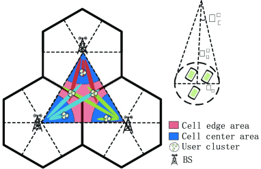
Figure 1: The Schematic of the IA-SSR based cooperative transmission scheme for the multi-cell massive MIMO systems.

II-B Spatially Correlated Channel Model in the Massive MIMO Networks

The downlink massive MIMO channels from $BS_{i}$ to the user $UE_{j,k}$ can be denoted as the $N_{r}\times N_{t}$ matrix $\mathbf{H}_{j,k}^{i}$, which are assumed to be block fading. Consider the classical “one-ring” model [22, 23], where the cluster $j$, located at $D_{j}^{i}$ meters away from ${BS}_{i}$, is surrounded by a ring of scatterers with the radius $R_{j}$. Then, for the cluster $j$, the angle spread (AS) at ${BS}_{i}$ is

$$\Delta_{j}^{i}=\arctan(R_{j}/D_{j}^{i}).$$ (1)

Similar to the works [13, 11, 12, 14], the BSs are elevated at a very high amplitude, such that there is not enough local scattering around the BS antennas. In such cases, the spatial correlation introduced by BS antennas should be considered. Furthermore, it is reasonable to assume that channel matrices of different users are independent. Then, $\mathbf{H}_{j,k}^{i}$ can be represented by [24]

$$\left[\mathbf{H}_{j,k}^{i}\right]^{T}=\sqrt{\beta_{j,k}^{i}}{\left(\mathbf{R}_{j,k}^{i}\right)}^{1/2}\mathbf{W}_{j,k}^{i}(\mathbf{\Phi}_{j,k})^{T/2},$$ (2)

where $\beta_{j,k}^{i}$ is the large-scale fading coefficient; $\mathbf{R}_{j,k}^{i}$ and $\mathbf{\Phi}_{j,k}$ are the spatial correlation matrices at $BS_{i}$ and $UE_{j,k}$, respectively; $\mathbf{W}_{j,k}^{i}$ is $r_{j}^{i}\times N_{r}$ is a random matrix, whose entries are i.i.d complex Gaussian distributed with zero mean and unit variance. It is a fact that all the users in the same cluster share the same one-ring model parameters. As a result, the spatial correlation matrix satisfies $\mathbf{R}_{j,k}^{i}=\mathbf{R}_{j}^{i}$ for all the users in the cluster $j$. Following the methods in[12], we can derive

$$\left[\mathbf{R}_{j}^{i}\right]_{p,q}=\frac{1}{2\Delta_{j}^{i}}\int_{\theta_{j}^{i}-\Delta_{j}^{i}}^{\theta_{j}^{i}+\Delta_{j}^{i}}e^{\frac{-2i\pi(p-q)\sin(\alpha)\tau}{\lambda}}d\alpha{\color[rgb]{0,0,1},}$$ (3)

where $\theta_{j}^{i}$ is the azimuth angle corresponding to the central point of scatters ring, $\tau$ is the antenna element spacing, and $\lambda$ is the carrier wavelength.

Resorting to eigen-decomposition, we can obtain

$$\mathbf{R}_{j}^{i}=\mathbf{E}_{j}^{i}{\bm{{\Lambda}}_{j}^{i}}\big{(}\mathbf{E}_{j}^{i}\big{)}^{H},$$ (4)

where ${\bm{{\Lambda}}_{j}^{i}}$ is an $r_{j}^{i}\times r_{j}^{i}$ diagonal matrix with the nonzero eigenvalues of $\mathbf{{R}}_{j}^{i}$ as the main diagonal elements, $\mathbf{E}_{j}^{i}$ is the $N_{t}\times r_{j}^{i}$ tall unitary matrix constructed by the eigenvectors of $\mathbf{R}_{j}^{i}$ corresponding to the nonzero eigenvalues, and $r_{j}^{i}$ denotes the rank of $\mathbf{R}_{j}^{i}$. With the Karhunen-Loeve representation, the matrix $\big{[}\mathbf{H}_{j,k}^{i}\big{]}^{T}$ can be re-expressed as [8]

$$\left[\mathbf{H}_{j,k}^{i}\right]^{T}=\sqrt{\beta_{j,k}^{i}}\mathbf{E}_{j}^{i}{\left(\bm{{\Lambda}}_{j}^{i}\right)}^{\frac{1}{2}}\mathbf{W}_{j,k}^{i}(\mathbf{\Phi}_{j,k})^{T/2}.$$ (5)

Moreover, we define the $N_{r}K_{j}\times N_{t}$ matrix $\mathbf{H}_{j}^{i}=\big{[}(\mathbf{H}_{j,1}^{i})^{T},(\mathbf{H}_{j,2}^{i})^{T},\cdots,(\mathbf{H}_{j,K_{j}}^{i})^{T}\big{]}^{T}$ as the downlink channel matrix from the $BS_{i}$ to the cluster $j$.

Interestingly, it can be readily checked that $\left[\mathbf{R}_{j}^{i}\right]_{p,q}=\left[\mathbf{R}_{j}^{i}\right]_{p+1,q+1}$, which means that $\mathbf{R}_{j}^{i}$ is a Toeplitz matrix. In the massive MIMO system, as $N_{t}$ approaches the infinity, $\mathbf{R}_{j}^{i}$ asymptotically tends to be a circulant matrix, and $\mathbf{E}_{j}^{i}$ can be constructed by $r_{j}^{i}$ columns of the $N_{t}\times N_{t}$ unitary discrete Fourier transform (DFT) matrix $\mathbf{F}_{N_{t}}$ as [25]

$$\!\!\mathbf{E}_{j}^{i}=\big{[}\mathbf{f}_{n}:n\in\mathcal{I}_{j}^{i}\big{]}{\color[rgb]{0,0,1},}$$ (6)

where $\mathbf{f}_{n}$ represents the $n$-th column of $\mathbf{F}_{N_{t}}$, and the index set $\mathcal{I}_{j}^{i}$ can be written as

$$\mathcal{I}_{j}^{i}= \Big{\{}n:2n/N_{t}-1\in\big{[}\frac{\tau}{\lambda}\sin({\theta_{j}^{i}\!+\Delta_{j}^{i}}).$$

$$~{}~{}~{}~{}~{}~{}~{}~{}~{}\frac{\tau}{\lambda}\sin({\theta_{j}^{i}\!-\Delta_{j}^{i}})\big{]},n=0,1,\cdots,N_{t}-1\Big{\}}$$

$$= \Big{\{}n:n\in\big{[}N_{t}\frac{\tau}{\lambda}\sin({\theta_{j}^{i}\!+\Delta_{j}^{i}})+\frac{N_{t}}{2},$$

$$N_{t}\frac{\tau}{\lambda}\sin({\theta_{j}^{i}\!-\Delta_{j}^{i}})+\frac{N_{t}}{2}\big{]},n=0,1,\cdots,N_{t}-1\Big{\}}.$$ (7)

Then, $r^{i}_{j}$ equals the cardinality of the index set $\mathcal{I}_{j}^{i}$, i.e.,

$$r_{j}^{i}= \left|N_{t}\frac{\tau}{\lambda}\sin({\theta_{j}^{i}+\Delta_{j}^{i}})-N_{t}\frac{\tau}{\lambda}\sin({\theta_{j}^{i}-\Delta_{j}^{i}})\right|$$

$$= 2N_{t}\frac{\tau}{\lambda}\left|\cos({\theta_{j}^{i}})\right|\sin({\Delta_{j}^{i}})$$

$$= 2N_{t}\frac{\tau}{\lambda}\left|\cos({\theta_{j}^{i}})\right|\sin\big{(}\arctan(R_{j}/D_{j}^{i})\big{)}.$$ (8)

Since the AS $\Delta_{j}^{i}$ is relatively small, $\mathbf{R}_{j}^{i}$ possesses low rank property, i.e., $r_{j}^{i}\ll N_{t}$.

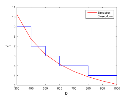
Figure 2: $r_{j}^{i}$ versus $D_{j}^{i}$ with $N_{t}=128,\theta_{j}^{i}=0^{\circ}$, and $R_{j}=25m$.

With (II-B), we can present the following theorem.

Theorem 1

In the one-ring channel model, if the parameter $R_{j}^{i}$ is fixed, the rank $r_{j}^{i}$ decreases with the increasing of the distance $D_{j}^{i}$.

To better understand Theorem 1, we present the curves of $r_{j}^{i}$ versus $D_{j}^{i}$ in Figure 2, where $N_{t}=128$, $\theta_{j}^{i}=0^{\circ}$, and $R_{j}=25m$. The red and blue curves are obtained from the closed-form expression in (II-B) and Monte Carlo numerical simulations, respectively. Figure 2 shows that the rank $r_{j}^{i}$ of $\mathbf{R}_{j}^{i}$ equals 9 for the clusters with $D_{j}^{i}=300m$, but reduces to 4 when $D_{j}^{i}$ increases to $900m$, which means that the rank of the channel covariances for the users in the cell-edge areas is obviously smaller than that for the cell-center users.

III Proposed IA-SSR Based Cooperative Transmission Scheme

In this section, the proposed transmission scheme will be presented under the two-stage precoding framework. Figure 1 shows the main idea of our proposed IA-SSR scheme. The coverage area of each sector is divided into the cell-center area and the cell-edge area. Correspondingly, the total coverage area can be partitioned into three different cell-center areas and one big cell-edge area, which consists of the edge areas of all the three sectors and is marked in red. Let us collect the clusters located in the cell-center area $i$ into the set $\mathcal{C}_{i}$, and gather the clusters within the cell-edge area into the set $\mathcal{E}$, i=1,2,3. To fully exploit the spatial DoF of the two-stage precoding, we will design different transmission schemes for the cell-edge and the cell-center clusters.

III-A IA Scheme for the Cell-edge Cluster

Obviously, the cluster in $\mathcal{E}$ has similar distance from each BS, and can be served by any of the three BSs. Hence, we let three BSs simultaneously transmit data to each cluster in $\mathcal{E}$ to enhance its data rate. For analysis simplicity, the number of the users in each cluster $j\in\mathcal{E}$ is assumed to be the same as that of BSs. Moreover, the data streams from each BS is intended for one specific user in cluster $j$. It should be pointed out that the cluster in $\mathcal{C}_{i}$ is still served only by $BS_{i}$. Under IA-SSR, the received signal of the cluster $j$ in $\mathcal{E}$ can be written as

$$\mathbf{y}_{j\in\mathcal{E}}= \sum_{i=1}^{3}\mathbf{H}_{j}^{i}\mathbf{x}^{i}+\mathbf{n}_{j}$$

$$= \sum_{i=1}^{3}\mathbf{H}_{j}^{i}\mathbf{P}_{j}^{i}\mathbf{d}_{j}^{i}+\sum_{i=1}^{3}\sum_{j^{\prime}\in\mathcal{E},j^{\prime}\neq j}\mathbf{H}_{j}^{i}\mathbf{P}_{j^{\prime}}^{i}\mathbf{d}_{j^{\prime}}^{i}$$

$$+\sum_{i=1}^{3}\sum_{j^{\prime}\in\mathcal{C}_{i}}\mathbf{H}_{j}^{i}\mathbf{P}_{j^{\prime}}^{i}\mathbf{d}_{j^{\prime}}^{i}+\mathbf{n}_{j},$$ (9)

where the $N_{t}\times 1$ vector $\mathbf{x}^{i}=\sum\limits_{j\in\mathcal{E}\cup\mathcal{C}_{i}}\mathbf{P}_{j}^{i}\mathbf{d}_{j}^{i}$ is the transmitted signal vector from $BS_{i}$, $\mathbf{d}_{j}^{i}$ is the $S^{i}_{j}\times 1$ data vector from the $BS_{i}$ to the cluster $j$, $\mathbf{P}_{j}^{i}$ is the $N_{t}\times S_{j}^{i}$ precoding matrix for the cluster $j$ at $BS_{i}$, and the $N_{r}K_{j}\times 1$ vector $\mathbf{n}_{j}\!\sim\!\mathcal{CN}(\mathbf{0},\mathbf{I}_{N_{r}K_{j}})$ is the additive complex Gaussian noise. Clearly, the first part on right hand side (RHS) of (III-A) is the superposition of the desired signals from the three BSs; the second and third parts are the inter-cluster interferences caused by the signals for other clusters in $\mathcal{E}$ and for clusters in $\mathcal{C}_{1}$ $\mathcal{C}_{2}$ and $\mathcal{C}_{3}$, respectively.

In this paper, we adopt the two-stage precoding framework, and divide the the precoding process into two stages as

$$\mathbf{P}_{j}^{i}=\mathbf{B}_{j}^{i}\mathbf{V}_{j}^{i},$$ (10)

where the $N_{t}\times M_{j}^{i}$ prebeamforming matrix $\mathbf{B}_{j}^{i}$, related to spatial correlation matrices, is utilized to eliminate the inter-cluster interferences; the $M_{j}^{i}\times S_{j}^{i}$ matrix $\mathbf{V}_{j}^{i}$ denotes the inner precoder dealing with the intra-cluster interferences, and depends on $K_{j}N_{r}\times M^{i}_{j}$ effective equivalent channel matrix $\overline{\mathbf{H}}_{j}^{i}={\mathbf{H}}_{j}^{i}\mathbf{B}^{i}_{j}$; $M_{j}^{i}$ is the rank of $\overline{\mathbf{H}}_{j}^{i}$ seen by the inner precoder, and satisfies the constraint $S_{j}^{i}\leq M_{j}^{i}\leq r_{j}^{i}$.

The design of the prebeamforming matrix $\mathbf{B}^{i}_{j}$ has been examined in [8, 9, 10, 11, 13, 12, 14]. Without loss of generality, we adopt the DFT based prebeamforming, and achieve the prebemforming matrices through concentrating the subspace $\text{span}\{\mathbf{B}^{i}_{j}\}$ into the null-space of $\text{span}\{\mathbf{\Xi}_{j}^{i}\}$, where $\mathbf{\Xi}_{j}^{i}$ is constructed by $\mathbf{E}_{j^{\prime}}^{i}$ of all but the cluster $j$ in the system as

$${\mathbf{\Xi}_{j}^{i}}=\Bigg{[}\mathbf{f}_{n}:n\in\bigcup_{j^{\prime}=1,j^{\prime}\neq j}^{J}\mathcal{I}_{j^{\prime}}^{i}\Bigg{]}.$$ (11)

With the orthogonality between any two columns of the DFT matrix, ${\mathbf{B}_{j}^{i}}$ for cluster $j$ in $\mathcal{E}$ can be derived as

$${\mathbf{B}_{j\in\mathcal{E}}^{i}}=\Bigg{[}\mathbf{f}_{n}:n\in\Bigg{(}\mathcal{I}_{j}^{i}-\bigcup_{j^{\prime}=1,j^{\prime}\neq j}^{J}\mathcal{I}_{j^{\prime}}^{i}\Bigg{)}\Bigg{]},$$ (12)

where the set $\mathcal{A}-\mathcal{B}$ contains all the elements that are in the set $\mathcal{A}$ but not in the set $\mathcal{B}$, i.e., $\mathcal{A}-\mathcal{B}=\{x:x\in\mathcal{A}\text{ and }x\notin\mathcal{B}\}$. From the computation of $\mathbf{B}_{j}^{i}$, we can obtain that $M_{j}^{i}$ equals the amount of the corresponding columns in $\mathbf{E}_{j}^{i}$ linearly independent on the ones of $\mathbf{\Xi}_{j}^{i}$ as

$$M^{i}_{j}=\text{rank}\{\mathbf{B}_{j}^{i}\}=\Bigg{|}\mathcal{I}_{j}^{i}-\bigcup_{j^{\prime}=1,j^{\prime}\neq j}^{J}\mathcal{I}_{j^{\prime}}^{i}\Bigg{|},$$ (13)

where $|\mathcal{A}|$ denotes the number of elements in the set $\mathcal{A}$. The resultant prebeamforming matrices $\mathbf{B}^{i}_{j}$ satisfy the following constraint as

$$\left\{\mathbf{E}_{j^{\prime}}^{i}\right\}^{H}{\mathbf{B}^{i}_{j}}=0,\forall j^{\prime}\neq j,$$ (14)

which means that the transmitted signal to the cluster $j\in\mathcal{E}$ will not cause interference to the other clusters. Then the inter-cluster interference terms in (III-A) are eliminated, and the received signals can be simplified as

$$\mathbf{y}_{j\in\mathcal{E}}= \sum_{i=1}^{3}\mathbf{\overline{H}}_{j}^{i}\mathbf{V}_{j}^{i}\mathbf{d}_{j}^{i}+\mathbf{n}_{j}.$$ (15)

The next task is to recover the intended data from the superimposed signals of the three BSs. We can separately present the received signal of each user as

$$\mathbf{y}_{j,1}= \overline{\mathbf{H}}_{j,1}^{1}\mathbf{V}_{j}^{1}\mathbf{d}_{j}^{1}+\sum_{i=2,3}\overline{\mathbf{H}}_{j,1}^{i}\mathbf{V}_{j}^{i}\mathbf{d}_{j}^{i}+\mathbf{n}_{j,1},$$ (16)

$$\mathbf{y}_{j,2}= \overline{\mathbf{H}}_{j,2}^{2}\mathbf{V}_{j}^{2}\mathbf{d}_{j}^{2}+\sum_{i=1,3}\overline{\mathbf{H}}_{j,2}^{i}\mathbf{V}_{j}^{i}\mathbf{d}_{j}^{i}+\mathbf{n}_{j,2},$$ (17)

$$\mathbf{y}_{j,3}= \overline{\mathbf{H}}_{j,3}^{3}\mathbf{V}_{j}^{3}\mathbf{d}_{j}^{3}+\sum_{i=1,2}\overline{\mathbf{H}}_{j,3}^{i}\mathbf{V}_{j}^{i}\mathbf{d}_{j}^{i}+\mathbf{n}_{j,3},$$ (18)

where $\mathbf{y}_{j,i}$ is the received signal of $U\!E_{j\in\mathcal{E},i}$ and contains the elements in $\mathbf{y}_{j\in\mathcal{E}}$ corresponding to $U\!E_{j\in\mathcal{E},i}$. Obviously, the first terms on the right hand side of (16)-(18) are the desired signals for each user, while the second terms represents the interference. With prebeamforming and cooperative transmission, the equivalent channel links from $BS_{1}$, $BS_{2}$ and $BS_{3}$ to the cluster $j\in\mathcal{E}$ become one three-BS three-user MIMO interference channel[26], where IA can be used to fully exploit the spatial freedoms.

Under the IA framework, the precoding matrix $\mathbf{V}_{j}^{i}$ can be carefully chosen to compact the interference into one reduced-dimensional subspace at the user side, but to keep the desired signals in another subspace. Thus, $\mathbf{V}_{j}^{i}$ should satisfy the following equation set [16]:

$$\overline{\mathbf{H}}_{j,1}^{3}\mathbf{V}_{j}^{3}= \overline{\mathbf{H}}_{j,1}^{2}\mathbf{V}_{j}^{2},$$ (19)

$$\overline{\mathbf{H}}_{j,2}^{3}\mathbf{V}_{j}^{3}= \overline{\mathbf{H}}_{j,2}^{1}\mathbf{V}_{j}^{1},$$ (20)

$$\overline{\mathbf{H}}_{j,3}^{1}\mathbf{V}_{j}^{2}= \overline{\mathbf{H}}_{j,3}^{1}\mathbf{V}_{j}^{1}.$$ (21)

Correspondingly, the columns of the decoding matrix $\mathbf{U}_{j,i}$ should be orthogonal to the subspace of the interference. Then, each user can derive $\mathbf{U}_{j,i}$ as

$$\mathbf{U}_{j,i}=\text{NULL}\left\{\sum_{k\neq i}\overline{\mathbf{H}}_{j,i}^{k}\mathbf{V}_{j}^{k}\right\},$$ (22)

where NULL$\{\mathbf{X}\}$ represents the nullspace of $\mathbf{X}$.

To ensure that IA is feasible, the following conditions should be satisfied [29].

$$\text{rank}\big{\{}(\mathbf{U}_{j,i})^{H}\overline{\mathbf{H}}_{j,i}^{i}\mathbf{V}_{j}^{i}\big{\}}=S_{j}^{i},$$ (23)

$$(\mathbf{U}_{j,i})^{H}\overline{\mathbf{H}}_{j,i}^{i^{\prime}}\mathbf{V}_{j}^{i^{\prime}}=\mathbf{0},\forall i\neq i^{\prime}.$$ (24)

After the IA operation, the interference is completely eliminated, and the received signal at the user $<\!\!j\!\!\in\!\mathcal{E},i\!>$ can be expressed as

$$\underline{\mathbf{y}}_{j\in\mathcal{E},i}=\underline{\mathbf{H}}_{j,i}^{i}\mathbf{d}_{j}^{i}+\underline{\mathbf{n}}_{j,i}{\color[rgb]{0,0,1},}$$ (25)

where $\underline{\mathbf{y}}_{j,i}=(\mathbf{U}_{j,i})^{H}{\mathbf{y}}_{j,i}$, $\underline{\mathbf{H}}_{j,i}^{i}=(\mathbf{U}_{j,i})^{H}\overline{\mathbf{H}}_{j,i}^{i}\mathbf{V}_{j}^{i}$ is the $S_{j}^{i}\times S_{j}^{i}$ full rank equivalent channel from $BS_{i}$ to the user $<\!\!j\!\!\in\!\mathcal{E},i\!>$, and the distribution characteristics of the equivalent noise $\underline{\mathbf{n}}_{j,i}=({\mathbf{U}}_{j,i})^{H}{\mathbf{n}}_{j,i}$ are the same with that of ${\mathbf{n}}_{j,i}$.

Remark 1

Under the IA based cooperative transmission, the transmitted signals from the three $BS$s to the cluster $j^{\prime}(j^{\prime}\neq j)$ are designed to avoid interference to the cluster $j\in\mathcal{E}$. Thus, it can be concluded that if the $BS_{1}$ is transmitting data to cluster $j$, $BS_{2}$ and $BS_{3}$ can also transmit data to the cluster $j$, and cause no impact on the other clusters they are serving. Therefore, the IA based cooperative transmission for the cell-edge clusters can fully exploit spatial DoF of the two-stage precoding in a multi-cell system.

Remark 2

IA is a promising interference management technology for a multi-cell cellular system. However, BS requires the global CSI, which will lead to unaffordable signaling overhead in the massive MIMO system due to its high dimensional channels. Fortunately, the two-stage precoding can significantly reduce the equivalent channel dimensions, which makes it possible to perform IA on the low dimensional equivalent channels $\overline{\mathbf{H}}_{j}^{i}$. Then, IA improves the data rate for cell-edge users under two-stage precoding. It can be concluded that the incorporation between IA and the two-stage precoding is a potential interference management technology with an affordable signal overhead over the multi-cell massive MIMO systems.

Remark 3

In contrast with existing cooperation methods [27, 28, 15], which share both CSI and user data streams among different BSs, the proposed scheme only shares CSI and can reduce the amount of signaling overhead along the backhaul links between the BSs.

To meet conditions (23) and (24), the number of the data streams should satisfy [29]

$$S^{i}_{j}\leq\min(M^{i}_{j},N_{r}),$$ (26)

$$\sum_{i=1}^{3}S^{i}_{j}(M^{i}_{j}+N_{r}-2S^{i}_{j})\geq S^{1}_{j}S^{2}_{j}+S^{2}_{j}S^{3}_{j}+S^{1}_{j}S^{3}_{j},$$ (27)

$$S^{i}_{j}+S^{i^{\prime}}_{j}\leq$$

$$\min\big{(}M^{i}_{j}+M^{i^{\prime}}_{j},2N_{r},\max(M^{i}_{j},N_{r}),\max(M^{i^{\prime}}_{j},N_{r})\big{)}.$$ (28)

Then, the optimal spatial DoF can be obtained by solving the following optimization problem:

$$(\text{P}1)~{}~{}~{}~{}~{}~{}~{}~{} \max_{S^{1}_{j},S^{2}_{j},S^{3}_{j}}S^{1}_{j}+S^{2}_{j}+S^{3}_{j}$$

$$~{}~{}{\text{s.t.}}\text{$~{}~{}~{}$\eqref{IA_constrains1}, \eqref{IA_constrains2}, \eqref{IA_constrains3}},$$

whose solution can be found the exhaustive search. The corresponding search complexity is $\prod\limits_{i=1}^{3}\big{[}\min(M^{i}_{j},N_{r})\big{]}$ and affordable.

III-B SSR Scheme for the Cell-center Cluster

In the IA-SSR, the received signal of the cluster $j$ in $\mathcal{C}_{i}$ can be written as

$${\mathbf{y}_{j\in\mathcal{C}_{i}}}=\mathbf{H}_{j}^{i}\mathbf{B}_{j}^{i}\mathbf{V}_{j}^{i}\mathbf{d}_{j}^{i}+\sum_{j^{\prime}\in\mathcal{C}_{i},j^{\prime}\neq j}\mathbf{H}_{j}^{i}\mathbf{B}_{j^{\prime}}^{i}\mathbf{V}_{j^{\prime}}^{i}\mathbf{d}_{j^{\prime}}^{i}$$

$$+\sum_{i^{\prime}=1}^{3}\sum_{j^{\prime}\in\mathcal{E}}\!\!\mathbf{H}_{j}^{i^{\prime}}\mathbf{B}_{j^{\prime}}^{i^{\prime}}\mathbf{V}_{j^{\prime}}^{i^{\prime}}\mathbf{d}_{j^{\prime}}^{i^{\prime}}+\!\!\!\!\sum_{i^{\prime}\!=1,i^{\prime}\!\neq i}^{3}\sum_{j^{\prime}\in\mathcal{C}_{i^{\prime}}}\!\!\mathbf{H}_{j}^{i^{\prime}}\mathbf{B}_{j^{\prime}}^{i^{\prime}}\mathbf{V}_{j^{\prime}}^{i^{\prime}}\mathbf{d}_{j^{\prime}}^{i^{\prime}}\!\!+\!\mathbf{n}_{j},$$ (29)

where the first part on the RHS of the above equation is the desired signal; the second and third parts are the interferences caused by the streams from $BS_{i}$ to the other clusters in $\mathcal{C}_{i}$ and from $BS_{1}$, $BS_{2}$ and $BS_{3}$ to the clusters in $\mathcal{E}$, respectively; the fourth part is the interference caused by streams for clusters in the other two cell-center areas.

The main operations of SSR can be presented as follows. The $BS_{i}$ loads one high-level power on the streams from the $BS_{i}$ to the clusters in $\mathcal{E}$, but assigns one low-level power for the streams to the clusters in $\mathcal{C}_{i}$. Since the distance between two cell-center areas is long enough to ensure the large path loss, the mutual-interference between two clusters in different cell-centers is low enough to be treated as noise.

With SSR, the data streams to one specific cluster in $\mathcal{C}_{i}$ should be optimized to avoid interference with the clusters in both $\mathcal{C}_{i}$ and $\mathcal{E}$ but not in $\mathcal{C}_{i^{\prime}}$, $i\neq i^{\prime}$. Then, for DFT based prebeamforming, the subspace $\text{span}\{\mathbf{B}_{j\in\mathcal{C}_{i}}^{i}\}$ should be orthogonal with the subspace span$\{\mathbf{\Psi}_{j}^{i}\}$ other than $\text{span}\{\mathbf{\Xi}_{j}^{i}\}$ in (11), where $\mathbf{\Psi}_{j}^{i}$ is constructed by $\mathbf{E}_{j^{\prime}}^{i}$ of all clusters but $j$ in $\mathcal{C}_{i}$ and those in $\mathcal{E}$ as

$${\mathbf{\Psi}_{j}^{i}}=\Bigg{[}\mathbf{f}_{n}:n\in\bigcup_{j^{\prime}\in\mathcal{C}_{i}\cup\mathcal{E},j^{\prime}\neq j}\mathcal{I}_{j^{\prime}}^{i}\Bigg{]}.$$ (30)

Then, we can derive the prebeamforming matrix for the cluster $j$ in $\mathcal{C}_{i}$ as

$${\mathbf{B}_{j\in\mathcal{C}_{i}}^{i}}=\Bigg{[}\mathbf{f}_{n}:n\in\Bigg{(}\mathcal{I}_{j}^{i}-\bigcup_{j^{\prime}\in\mathcal{C}_{i}\cup\mathcal{E},j^{\prime}\neq j}\mathcal{I}_{j^{\prime}}^{i}\Bigg{)}\Bigg{]}.$$ (31)

After prebeamforming, the received signal in (III-B) can be simplified as

$${\mathbf{y}_{j\in\mathcal{C}_{i}}}= \mathbf{\overline{H}}_{j}^{i}\mathbf{V}_{j}^{i}\mathbf{d}_{j}^{i}+\underline{\mathbf{n}}_{j},$$ (32)

where

$$\underline{\mathbf{n}}_{j}=\sum_{i^{\prime}\!=1,i^{\prime}\!\neq i}^{3}\sum_{j^{\prime}\in\mathcal{C}_{i^{\prime}}}\!\!\mathbf{H}_{j}^{i^{\prime}}\mathbf{B}_{j^{\prime}}^{i^{\prime}}\mathbf{V}_{j^{\prime}}^{i^{\prime}}\mathbf{d}_{j^{\prime}}^{i^{\prime}}\!\!+\!\mathbf{n}_{j}{\color[rgb]{0,0,1},}$$ (33)

denotes the equivalent noise, and its conditional covariance matrix on given $\{\mathbf{H}_{j}^{i^{\prime}}\mathbf{B}_{j^{\prime}}^{i^{\prime}}\}$ is denoted by $\mathbf{K}_{j\in\mathcal{C}_{i}}$.

For given $\mathbf{B}_{j}^{i}$, $\mathbf{\overline{H}}_{j}^{i}$ represents the traditional multiuser MIMO broadcast channel [30], and the ZF inner precoder can be utilized to deal with intra-cluster interference [31]. The detailed ZF inner precoder can be written as

$$\mathbf{V}_{j}^{i}=\zeta_{j}^{i}\mathbf{{Z}}_{j}^{i},$$ (34)

where $\mathbf{{Z}}_{j}^{i}=\big{(}\mathbf{\overline{H}}_{j}^{i}\big{)}^{H}\left(\mathbf{\overline{H}}_{j}^{i}\big{(}\mathbf{\overline{H}}_{j}^{i}\big{)}^{H}\right)^{-1}$, and $\zeta_{j}^{i}=\sqrt{\frac{S_{j}^{i}}{\text{tr}\left(\mathbf{{Z}}_{j}^{i}\left(\mathbf{{Z}}_{j}^{i}\right)^{H}\right)}}$ is a normalization factor to constrain the power gain of inner precoder.

After the ZF inner precoding, the received signal of the cell-center cluster in (32) can be rewritten as

$${\mathbf{y}_{j\in\mathbb{C}_{i}}}= \mathbf{\underline{H}}_{j}^{i}\mathbf{d}_{j}^{i}+\underline{\mathbf{n}}_{j},$$ (35)

where $\underline{\mathbf{H}}_{j}^{i}=\overline{\mathbf{H}}_{j}^{i}\mathbf{V}_{j}^{i}=\zeta_{j}^{i}\mathbf{I}_{S_{j}^{i}}$ is the $S_{j}^{i}\times S_{j}^{i}$ equivalent channel for the cluster $j$ in the $\mathcal{C}_{i}$.

Under SSR, $M_{j}^{i}$ equals the number of columns in $\mathbf{E}_{j}^{i}$ that are linearly independent on the columns of $\mathbf{\Psi}_{j}^{i}$. The number of the data streams from $BS_{i}$ to the cluster $j\in\mathcal{C}_{i}$ is given by

$$S^{i}_{j\in\mathcal{C}_{i}} =M^{i}_{j\in\mathcal{C}_{i}}=\text{rank}\{\mathbf{B}_{j}^{i}\}=\Bigg{|}\mathcal{I}_{j}^{i}-\bigcup_{j^{\prime}\in\mathcal{C}_{i}\cup\mathcal{E},j^{\prime}\neq j}\mathcal{I}_{j^{\prime}}^{i}\Bigg{|}.$$ (36)

Comparing with the scenario without SSR in (13), the number of data streams for the cell-center clusters may be significantly improved, which can be explained as follows. When SSR is not adopted, if the AoD range of the cluster $j\in\mathcal{C}_{i}$ overlaps with that of the cluster $j^{\prime}\in\mathcal{C}_{i^{\prime}}$ at $BS_{i}$, $BS_{i}$ should not transmit data streams for the cluster $j\in\mathcal{C}_{i}$ on the overlapping beams in order to avoid interference. Nonetheless, if we utilize SSR, $BS_{i}$ can transmit data streams to the cluster $j\in\mathcal{C}_{i}$, while $BS_{i^{\prime}}$ can simultaneously transmit data streams to $j^{\prime}\in\mathcal{C}_{i^{\prime}}$.

Remark 4

With the SSR scheme, the AoD range overlapping is mitigated since the mutual-interference between two clusters in different cell-centers is negligible. Thus, we do not need to treat all the clusters in the whole system as one big group anymore. However, the mutual-interference between cell-center clusters and cell-edge clusters sill exists. Therefore, for the cluster $j\in\mathcal{E}$, its prebeamforming should still be well designed to avoid interference with all the other clusters in the system.

III-C Power Allocation for IA-SSR

In this section, we will develop a power allocation policy for the proposed IA-SSR scheme to maximize the sum-capacity. Thanks to the two-stage precoding scheme, the channel links for the whole system can be decomposed into several independent equivalent channel links with reduced dimensions, as shown in (25) and (35). Let us assume that BSs have knowledge of the effective equivalent channels $\{\underline{\mathbf{H}}_{j}^{i}\}$ and the equivalent noise covariance matrices $\{\mathbf{K}_{j\in\mathcal{C}_{i}}\}$. Then, the achievable capacity of the link from $BS_{i}$ to the cluster $j$ in $\mathcal{E}$ can be expressed as [32]

$$\mathbb{C}_{j\in\mathcal{E},i}^{i}\left(\underline{\mathbf{H}}_{j,i}^{i}\right) =\log\det\Big{\{}\mathbf{I}_{S_{j}^{i}}+\left(\underline{\mathbf{H}}_{j,i}^{i}\right)\mathbf{Q}_{j}^{i}\left(\underline{\mathbf{H}}_{j,i}^{i}\right)^{H}\Big{\}}$$

$$=\sum_{s=1}^{S_{j}^{i}}\log\left\{1+\lambda_{j,s}^{i}p_{j,s}^{i}\right\},$$ (37)

where $\lambda_{j,s}^{i}$ is the $s$-th eigenvalue of $\underline{\mathbf{H}}_{j,i}^{i}(\underline{\mathbf{H}}_{j,i}^{i})^{H}$, $\mathbf{Q}_{j}^{i}=\mathbb{E}\left\{\mathbf{d}_{j}^{i}(\mathbf{d}_{j}^{i})^{H}\right\}$, and its $s$-th eigenvalue $p_{j,s}^{i}$ represents the transmitting power for the $s$-th data stream from $BS_{i}$ to the cluster $j$.

Similarly, the achievable capacity of the link from $BS_{i}$ to the cluster $j$ in $\mathcal{C}_{i}$ can be written as

$${\mathbb{C}_{j\in\mathcal{C}_{i}}^{i}}\left(\underline{\mathbf{H}}_{j}^{i}\right) =\log\det\Big{\{}\mathbf{I}+\mathbf{K}_{j}^{-1}\left(\underline{\mathbf{H}}_{j}^{i}\right)\mathbf{Q}_{j}^{i}\left(\underline{\mathbf{H}}_{j}^{i}\right)^{H}\Big{\}}$$

$$=\sum_{s=1}^{S_{j}^{i}}\log\left\{1+k_{j,s}^{-1}\left(\zeta_{j}^{i}\right)^{2}p_{j,s}^{i}\right\},$$ (38)

where $k_{j,s}$ is $s$-th eigenvalue of $\mathbf{K}_{j}$. In IA-SSR, $BS_{i}$ serves all the clusters in $\mathcal{C}_{i}$ and the $i$-th user of each cluster in $\mathcal{E}$. Then, the achievable sum-capacity of the whole system can be listed as

$$\mathbb{C}_{sum}=\sum_{i=1}^{3}\Bigg{(}\sum_{j\in\mathcal{C}_{i}}\mathbb{C}_{j}^{i}+\sum_{j\in\mathcal{E}}\mathbb{C}_{j,i}^{i}\Bigg{)}.$$ (39)

As mentioned in the above subsection, we load one low-level power $p_{cent}$ on each data stream for the cell-center clusters to avoid the mutual-interference between different cell-centers, i.e., $p_{j\in\mathcal{C}_{i},s}^{i}=p_{cent}$. To maximize the sum-capacity of the network, the optimization problem with respect to both $p_{cent}$ and ${p}_{j\in\mathcal{E},s}^{i}$ can be formulated as

$$(\text{P}2) \max_{p_{cent},~{}{p}_{j\in\mathcal{E},s}^{i}}\mathbb{C}_{sum}$$ (40)

s.t. $$\sum_{i=1}^{3}\Big{(}\sum_{j\in\mathcal{C}_{i}}\sum_{s=1}^{S_{j}^{i}}p_{cent}+\sum_{j\in\mathcal{E}}\sum_{s=1}^{S_{j}^{i}}p_{j,s}^{i}\Big{)}\leq P_{total},$$

$$p_{cent}\geq 0,$$

$$p_{j\in\mathcal{E},s}^{i}\geq 0,$$

where $P_{total}$ is the total power. Unfortunately, since the equivalent noise of the cell-center cluster is dependent on $p_{cent}$, the classical water-filling algorithm cannot be used to solve the above problem. Nonetheless, for the given $p_{cent}$, the problem (P2) can be simplified as

$$(\text{P}3)~{}~{}~{}~{}~{}~{}~{}~{}\max_{{p}_{j\in\mathcal{E},s}^{i}}\mathbb{C}_{sum,\mathcal{E}} =\sum_{i=1}^{3}\sum_{j\in\mathcal{E}}\mathbb{C}_{j,i}^{i}$$ (41)

$${\text{s.t.}}~{}~{}~{}\sum_{i=1}^{3}\sum_{j\in\mathcal{E}}\sum_{s=1}^{S_{j}^{i}}p_{j,s}^{i} \leq P_{total}-\sum_{i=1}^{3}\sum_{j\in\mathcal{C}_{i}}\sum_{s=1}^{S_{j}^{i}}p_{cent},$$

$$p_{j\in\mathcal{E},s}^{i} \geq 0.$$

With the Karush-Kuhn-Tucker condition, we can achieve the solution for (P3) as

$$p_{j\in\mathcal{E},s}^{i} =\max{\left\{0,\frac{1}{\mu}-\frac{1}{\lambda_{j,s}^{i}}\right\}},$$ (42)

where $\mu$ is the Lagrange multiplier factor and satisfies

$$\sum_{i=1}^{3}\sum_{j\in\mathcal{E}}\sum_{s=1}^{S_{j}^{i}}\max{\left\{0,\frac{1}{\mu}-\frac{1}{\lambda_{j,s}^{i}}\right\}}$$

$$~{}~{}~{}~{}~{}~{}~{}~{}~{}~{}~{}~{}~{}~{}~{}~{}=P_{total}-\sum_{i=1}^{3}\sum_{j\in\mathcal{C}_{i}}\sum_{s=1}^{S_{j}^{i}}p_{cent}.$$ (43)

According to (42) and (43), the water-filling algorithm can be adopted to perform the power allocation for the cell-edge clusters with given $p_{cent}$.

Obviously, the sum-capacity $\sum\limits_{i=1}^{3}\sum\limits_{j\in\mathcal{E}}\mathbb{C}_{j,i}^{i}$ of the cell-edge clusters always decreases with the increase of $p_{cent}$. Moreover, when $p_{cent}$ lies in a small regime, the sum-capacity of the cell-center cluster $\sum\limits_{i=1}^{3}\sum_{j\in\mathcal{C}_{i}}\mathbb{C}_{j,i}^{i}$ is proportional to $p_{cent}$. However, when $p_{cent}$ lies in a large regime, the interference between different cell-centers will be introduced, and the sum-capacity of the cell-center cluster will be limited by the interference. Therefore, with the increase of $p_{cent}$, $\mathbb{C}_{sum}$ first increases and then decreases. With this property, we will utilize the golden section method to solve the power allocation problem (P2), which is described in Algorithm 1 [33].

Algorithm 1 Power Allocation Algorithm

1:  Initialize maximum tolerance $\varepsilon$, set $p_{l}=0,p_{r}=\frac{P_{total}}{\sum_{i=1}^{3}\sum_{j\in\mathcal{C}_{i}}S_{j}^{i}}$.

2:  repeat

3:     $p_{m1}=p_{l}+0.382|p_{r}-p_{l}|$;solve problem (P3) for a given $p_{cent}=p_{m1}$ and obtain power allocation policies $\{{p}_{j\in\mathcal{E},s}^{i}\}_{1}$; calculate ${\mathbb{C}_{sum}}_{1}$ through (39).

4:     $p_{m2}=p_{l}+0.618|p_{r}-p_{l}|$;solve problem (P3) for a given $p_{cent}=p_{m2}$ and obtain power allocation policies $\{{p}_{j\in\mathcal{E},s}^{i}\}_{2}$; calculate ${\mathbb{C}_{sum}}_{2}$ through (39).

5:     if ${\mathbb{C}_{sum}}_{1}>{\mathbb{C}_{sum}}_{2}$ then

6:        $p_{l}=p_{m1}$; $p_{cent}=p_{m1};\{p_{j\in\mathcal{E},s}^{i}\}=\{{p}_{j\in\mathcal{E},s}^{i}\}_{1}$.

7:     else

8:        $p_{r}=p_{m2}$; $p_{cent}=p_{m2};\{p_{j\in\mathcal{E},s}^{i}\}=\{{p}_{j\in\mathcal{E},s}^{i}\}_{2}$.

9:     end if

10:  until $|p_{r}-p_{l}|<\varepsilon$

11:  return   $p_{cent},\{p_{j\in\mathcal{E},s}^{i}\}$

IV The Channel Estimation for IA-SSR

In order to design the prebeamforming matrices, BSs need to acquire the channel eigenspaces $\mathbf{E}_{j}^{i}$ of each cluster. From (4), we know that the spatial correlation matrix of a cluster is determined by its AoD and AS, which change slowly with respect to the channel coherent time [34]. Moreover, the uplink-downlink reciprocity exists for spatial correlation matrix even in the FDD system [35]. Hence, $\{\mathbf{E}_{j}^{i}\}$ can be tracked from the uplink training with low overhead [36]. Here, we assume that $\{\mathbf{E}_{j}^{i}\}$ is available to BSs.

In the FDD system, unlike $\{\mathbf{E}_{j}^{i}\}$, the effective equivalent channel $\{\overline{\mathbf{H}}_{j}^{i}\}$ should be obtained through the downlink training and the user feedback within each channel coherent block, which accounts for the major part of the total signaling overhead in IA-SSR. In order to estimate $\overline{\mathbf{H}}_{j}^{i}$ and $\mathbf{K}_{j\in\mathcal{C}_{i}}$ in a low-overhead way, we propose a training scheme to reuse the training matrices within each BS, where the linear least squares (LS) estimator is adopted. In our scheme, $BS_{i}$ transmits the training matrices $\mathbf{T_{e}}_{j}^{i}$ of size $M_{j}^{i}\times{T_{e}}_{j}$ and $\mathbf{T_{c}}_{i}^{j}$ of size $M_{j}^{i}\times{T_{c}}_{j}$, respectively.

IV-A The Estimation of the Effective Equivalent Channels $\{\overline{\mathbf{H}}_{j\in\mathcal{E}}^{i}\}$, $\{\overline{\mathbf{H}}_{j\in\mathcal{C}_{i}}^{i}\}$

It can be found that $\overline{\mathbf{H}}_{j}^{i}$ possesses a much smaller number of unknown parameters than the original channel matrix $\mathbf{H}_{j}^{i}$. As a result, the estimation of $\overline{\mathbf{H}}_{j}^{i}$ consumes less channel resource than estimation of $\mathbf{H}_{j}^{i}$. We first consider the estimation of $\mathbf{\overline{H}}_{j\in\mathcal{E}}^{i}$, $i=1,2,3$. Recalling the effective equivalent channel model in (15), the received training signal of the cluster $j$ in $\mathcal{E}$ is given by

$$\mathbf{Y}_{j\in\mathcal{E}}= \sum_{i=1}^{3}\mathbf{\overline{H}}_{j}^{i}\mathbf{T_{e}}_{j}^{i}+\mathbf{N}_{j}{\color[rgb]{0,0,1},}$$ (44)

where $\mathbf{N}_{j}=[{\mathbf{n}_{j}}_{1},{\mathbf{n}_{j}}_{2},\cdots,{\mathbf{n}_{j}}_{{T_{c}}_{j}}]$ contains the noise vectors of ${T_{c}}_{j}$ time slots. From the LS theory, to implement the optimal estimation of $\{\overline{\mathbf{H}}_{j\in\mathcal{E}}^{i}\}(i=1,2,3)$, the training matrices from the three BSs to a specific cluster $j$ in $\mathcal{E}$ should be orthogonal with each other, which means that

$$\mathbf{T_{e}}_{j}^{i}(\mathbf{T_{e}}_{j}^{i^{\prime}})^{H} =\mathbf{0},i\neq i^{\prime}.$$ (45)

Since the channel links from one specific BS to its served clusters are independent, the training matrices can be reused among different clusters. With this consideration, the minimal value of ${T_{e}}_{j}$ satisfying (45) is

$${T_{e}}_{j}=\sum\limits_{i=1}^{3}M_{j}^{i}.$$ (46)

Then, we focus on the estimation of $\mathbf{\overline{H}}_{j\in\mathcal{C}_{i}}^{i}$. Similarly, we can obtain the received training signal of the cluster $j$ in $\mathcal{C}_{i}$ as

$${\mathbf{Y}_{j\in\mathcal{C}_{i}}}= \mathbf{\overline{H}}_{j}^{i}\mathbf{T_{c}}_{j}^{i}+\sum_{i^{\prime}\!=1,i^{\prime}\!\neq i}^{3}\sum_{j^{\prime}\in\mathcal{C}_{i^{\prime}}}\!\!\mathbf{H}_{j}^{i^{\prime}}\mathbf{B}_{j^{\prime}}^{i^{\prime}}\mathbf{T_{c}}_{j^{\prime}}^{i^{\prime}}\!\!+\!\mathbf{N}_{j}.$$ (47)

To estimate $\overline{\mathbf{H}}_{j\in\mathcal{C}_{i}}^{i}$ in absence of interference, the training matrices for the clusters in the cell-center areas should satisfy

$$\mathbf{T_{c}}_{j}^{i}(\mathbf{T_{c}}_{j^{\prime}}^{i^{\prime}})^{H} =\mathbf{0},j\in\mathcal{C}_{i},j^{\prime}\in\mathcal{C}_{i^{\prime}},i\neq i^{\prime}.$$ (48)

Furthermore, the covariance matrix $\mathbf{K}_{j\in\mathcal{C}_{i}}$ of the equivalent noise in (33) can be achieved through estimating each interference channel $\mathbf{H}_{j}^{i^{\prime}}\mathbf{B}_{j^{\prime}}^{i^{\prime}}$, which will need large training matrices. To save training resources, we directly estimate the sum of interference channels instead of the respective channels. Then, the training resources can be reused within each BS, and only the orthogonality among training matrices from different BSs is required to satisfy (48). Therefore, the minimal dimension ${T_{c}}_{j}$ can be listed as

$${T_{c}}_{j}=\sum_{i=1}^{3}\bar{M}^{i},$$ (49)

where $\bar{M}^{i}=\max\limits_{j\in\mathcal{C}_{i}}M_{j}^{i}$. To make the proposed scheme more specific, we would like to show an example of the designed training matrices and the whole procedures of channel estimation. Here, we construct the training matrices for the cluster $j$ in $\mathcal{E}$ from the ${T_{e}}_{j}\times{T_{e}}_{j}$ DFT matrix $\mathbf{F}_{e}$ as

$$\mathbf{T_{e}}_{j}^{1}=\big{[}\mathbf{F}_{e}\big{]}_{1:M_{j}^{1},}$$ (50)

$$\mathbf{T_{e}}_{j}^{2}=\big{[}\mathbf{F}_{e}\big{]}_{M_{j}^{1}+1:(M_{j}^{1}+M_{j}^{2}),}$$ (51)

$$\mathbf{T_{e}}_{j}^{3}=\big{[}\mathbf{F}_{e}\big{]}_{M_{j}^{1}+M_{j}^{2}+1:(M_{j}^{1}+M_{j}^{2}+M_{j}^{3}),}$$ (52)

where $[\mathbf{A}]_{m:n}$ denotes the submatrix formed by the columns of $\mathbf{A}$ with indices from $m$ to $n$. Correspondingly, the training matrices for the cluster $j$ in $\mathcal{C}_{i}$ can be achieved from the ${T_{c}}_{j}\times{T_{c}}_{j}$ DFT matrix $\mathbf{F}_{c}$ as

$$\mathbf{T_{c}}_{j}^{i}=\big{[}\mathbf{F}_{c}^{i}\big{]}_{1:M_{j}^{i},}$$ (53)

where $\mathbf{F}_{c}^{i}$ is defined as

$$\mathbf{F}_{c}^{i}=\big{[}\mathbf{F}_{c}\big{]}_{1:\bar{M}^{1},}$$ (54)

$$\mathbf{F}_{c}^{2}=\big{[}\mathbf{F}_{c}\big{]}_{(\bar{M}^{1}+1):(\bar{M}^{1}+\bar{M}^{2}),}$$ (55)

$$\mathbf{F}_{c}^{3}=\big{[}\mathbf{F}_{c}\big{]}_{(\bar{M}^{1}+\bar{M}^{2}+1):(\bar{M}^{1}+\bar{M}^{2}+\bar{M}^{3}).}$$ (56)

Then, the LS estimation of $\overline{\mathbf{H}}_{j}^{i}$ can be formed as

$$\widehat{\overline{\mathbf{H}}}_{j\in\mathcal{E}}^{i} =\mathbf{Y}_{j\in\mathcal{E}}\{\mathbf{T_{e}}_{j}^{i}\}^{H}=\mathbf{\overline{H}}_{j\in\mathcal{E}}^{i}+\mathbf{N}_{j}\{\mathbf{T_{e}}_{j}^{i}\}^{H},$$ (57)

$$\widehat{\overline{\mathbf{H}}}_{j\in\mathcal{C}_{i}}^{i} =\mathbf{Y}_{j\in\mathcal{C}_{i}}\{\mathbf{T_{c}}_{j}^{i}\}^{H}=\mathbf{\overline{H}}_{j\in\mathcal{C}_{i}}^{i}+\mathbf{N}_{j}\{\mathbf{T_{c}}_{j}^{i}\}^{H},$$ (58)

where the equations (45), (48), and the properties $\mathbf{T_{e}}_{j}^{i}(\mathbf{T_{e}}_{j}^{i})^{H}=\mathbf{I}$, $\mathbf{T_{c}}_{j}^{i}(\mathbf{T_{c}}_{j}^{i})^{H}=\mathbf{I}$ are utilized.

IV-B The Recovering of the Covariance Matrices $\mathbf{K}_{j\in\mathcal{C}_{i}}$

We give the procedures for the estimation of $\mathbf{K}_{j\in\mathcal{C}_{i}}$ in this subsection. Multiplying $\mathbf{Y}_{j\in\mathcal{C}_{i}}$ by $\{\mathbf{F}_{c}^{i^{\prime}}\}^{H}$, we can obtain

$$\mathbf{\Upsilon}_{j\in\mathcal{C}_{i}} =\sum_{i^{\prime}\!=1,i^{\prime}\!\neq i}^{3}\mathbf{Y}_{j\in\mathcal{C}_{i}}\{\mathbf{F}_{c}^{i^{\prime}}\}^{H}$$

$$=\sum_{i^{\prime}\!=1,i^{\prime}\!\neq i}^{3}\mathbf{N}_{j}\{\mathbf{F}_{c}^{i^{\prime}}\}^{H}$$

$$~{}~{}~{}+\sum_{i^{\prime}\!=1,i^{\prime}\neq i}^{3}\sum_{j^{\prime}\in\mathcal{C}_{i^{\prime}}}\!\!\!\mathbf{H}_{j}^{i^{\prime}}\mathbf{B}_{j^{\prime}}^{i^{\prime}}\!\left[\mathbf{I}_{M_{j}^{i}},\!\mathbf{0}_{M_{j}^{i}\!\times(\bar{M}^{i}\!-\!M_{j}^{i})}\right],$$ (59)

where the facts that $\mathbf{T_{c}}_{j}^{i}\mathbf{F}_{c}^{i^{\prime}}=\mathbf{0}$ and $\mathbf{T_{c}}_{j}^{i}\mathbf{F}_{c}^{i}=[\mathbf{I}_{M_{j}^{i}},\mathbf{0}_{M_{j}^{i}\times(\bar{M}^{i}-M_{j}^{i})}]$ are utilized in the above derivation.

Resorting to the properties $\mathbf{N}_{j}(\mathbf{N}_{j})^{H}=\sum_{t=1}^{{T_{c}}_{j}}{{\mathbf{n}_{j}}_{t}}{\mathbf{n}_{j}}_{t}^{H}\approx{T_{c}}_{j}\mathbf{I}$, and $\left[\mathbf{I}_{M_{j}^{i}},\!\mathbf{0}_{M_{j}^{i}\!\times(\bar{M}^{i}\!-\!M_{j}^{i})}\right]\left[\mathbf{I}_{M_{j}^{i}},\!\mathbf{0}_{M_{j}^{i}\!\times(\bar{M}^{i}\!-\!M_{j}^{i})}\right]^{H}=\mathbf{I}_{M_{j}^{i}}$, we can derive

$$\mathbf{\Upsilon}_{j}(\mathbf{\Upsilon}_{j})^{H}$$

$$\!\!\approx\!\!2{T_{c}}_{j}\mathbf{I}+\underbrace{\!\!{\left(\sum_{i^{\prime}\!=1,i^{\prime}\!\neq i}^{3}\sum_{j^{\prime}\in\mathcal{C}_{i^{\prime}}}\!\!\!\mathbf{H}_{j}^{i^{\prime}}\mathbf{B}_{j^{\prime}}^{i^{\prime}}\right)\!\!\!\!\left(\sum_{i^{\prime}\!=1,i^{\prime}\!\neq i}^{3}\sum_{j^{\prime}\in\mathcal{C}_{i^{\prime}}}\!\!\!\mathbf{H}_{j}^{i^{\prime}}\mathbf{B}_{j^{\prime}}^{i^{\prime}}\right)^{H}}\!\!}_{\mathbf{\Sigma}_{j}}.$$

where ${\mathbf{\Sigma}_{j}}$ is the covariance matrix for the sum of all the interference channels. Since the power of each data stream for the cell-center cluster is $p_{cent}$, the covariance matrix of the equivalent noise $\underline{\mathbf{n}}_{i}$ in data transmission stage can be given by

$$\widehat{\mathbf{K}}_{j}=\mathbf{I} +p_{cent}\mathbf{\Sigma}_{j}$$

$$=\mathbf{I} +p_{cent}\big{(}\mathbf{\Upsilon}_{j}(\mathbf{\Upsilon}_{j})^{H}-2{T_{c}}_{j}\mathbf{I}\big{)}{\color[rgb]{0,0,1}.}$$ (60)

Remark 5

The proposed channel estimation scheme for IA-SSR requires low dimensional training matrices. Hence, our scheme eliminates the the pilot contamination [37], which hinders the performance of multi-cell massive MIMO systems.

V The Discussion about the Implementation of IA-SSR

V-A The Overhead Analysis

In the IA-SSR scheme, each cell-center cluster and each cell-edge cluster needs to feedback $M_{j}^{i}K_{j}N_{r}$ and $\sum\limits_{i=1}^{3}M_{j}^{i}K_{j}N_{r}$, respectively. Let us assume that each complex channel coefficient is quantized into $Q$ bits, the channel coherent block length is $T$, and the rate of the feedback channel is $F$ bits per symbol. Taking into consideration of the overhead of both the training and the feedback, we can separately derive the effective sum-rates for the cell-center cluster and the cell-edge cluster as

$$\mathbb{R}_{j\in\mathcal{C}_{i}}=\alpha_{j\in\mathcal{C}_{i}}\mathbb{C}_{j\in\mathcal{C}_{i}},~{}~{}~{}~{}~{}\mathbb{R}_{j\in\mathcal{E}}\!=\alpha_{j\in\mathcal{E}}\mathbb{C}_{j\in\mathcal{E}},$$ (61)

where

$$\alpha_{j\in\mathcal{C}_{i}} =\max\left\{1-\frac{{T_{c}}_{j}}{T}-\frac{M_{j}^{i}K_{j}N_{r}Q}{FT},0\right\},$$ (62)

$$\alpha_{j\in\mathcal{E}} =\max\left\{1-\frac{{T_{e}}_{j}}{T}-\frac{\sum_{i=1}^{3}M_{j}^{i}K_{j}N_{r}Q}{FT},0\right\}.$$ (63)

V-B Cluster division for IA-SSR

In the proposed transmission scheme, it is critical to divide the user clusters into the cell-­edge clusters and cell-­center cluster. To achieve a better performance, we would like to develop a adaptive clustering method. Theoretically, for a specific cluster $j$, we can separately derive its achievable capacity under two cases. The first one is that the cluster $j$ belongs to the cell-edge area, and the second one is that the cluster $j$ lies in the cell-center area. The capacity for the former case is denoted as $\mathbb{C}_{j\in\mathcal{E}}$ in (III-C), while that for the latter one is $\mathbb{C}_{j\in\mathcal{C}_{i}}$ in (III-C). Then, we can formulate the clustering method to maximize the achievable capacity of the whole system as

$$\left\{\begin{array}[]{ll}j\in\mathcal{E},~{}~{}\text{if}~{}\mathbb{C}_{j\in\mathcal{E}}>\mathbb{C}_{j\in\mathcal{C}_{i}};\\ j\in\mathcal{C}_{i^{*}},i^{*}=\arg\max\limits_{i}{\mathbb{C}_{j\in\mathcal{C}_{i}}},~{}~{}\text{otherwise}.\end{array}\right.$$ (66)

However, this scheme requires to estimate and feed back the equivalent channels $\{\underline{\mathbf{H}}_{j}^{i}\}$ between all the clusters and the three BSs, which would seriously degrade the effective system sum-rate. To deal with this challenges, we will develop a low-overhead cluster division criterion.

Recalling the optimal problem (P1), we list some examples of the optimal $({S^{1}_{j},S^{2}_{j},S^{3}_{j}})$ in Table I.

TABLE I: Optimal $S^{1}_{j},S^{2}_{j},S^{3}_{j}$ with Given $M^{1}_{j}$ , $M^{2}_{j}$ , $M^{3}_{j}$ and $N_{r}$.

($M^{1}_{j}$ , $M^{2}_{j}$ , $M^{3}_{j}$ , $N_{r}$)	$\sum_{i=1}^{3}{S^{i}_{j}}$	$(S^{1}_{j},S^{2}_{j},S^{3}_{j})$	IA efficient?
(2 , 2 , 2 , 2)	3	(1,1,1)	yes
(3 , 3 , 3 , 2)	4	(2,1,1)	yes
(5 , 3 , 3 , 2)	4	(2,1,1)	no
(4 , 4 , 4 , 4)	6	(2,2,2)	yes
(5 , 4 , 4 , 4)	6	(2,2,2)	yes
(7 , 4 , 4 , 4)	6	(2,2,2)	no

As observed from Table I, the IA-based cooperative transmission has many advantages, but it is not always suitable for all the clusters. Obviously, IA is efficient if the following condition holds,

$$S^{1}_{j}+S^{2}_{j}+S^{3}_{j}>\max(M^{1}_{j},M^{2}_{j},M^{3}_{j}),$$ (67)

which means that the IA-based cooperative transmission provides more data streams than the transmission from a single BS. Otherwise, the cluster $j$ should be served by $BS_{i}$ with maximal $M^{i}_{j}$ exclusively.

Generally, IA is efficient if $M^{1}_{j},M^{2}_{j}$ and $M^{3}_{j}$ is roughly same. According to Theorem 1, $M^{i}_{j}$ is closely related to the distance from $BS_{i}$ to the cluster $j$. With this result, we can achieve that IA is efficient for the cell-edge cluster, which have similar distance from each BS. However, $M^{i}_{j}$ is obviously greater than $M^{i^{\prime}}_{j}$ for the cluster $j$ in the cell-center area $i$, $i^{\prime}\neq i$. In this case, $BS_{i}$ exclusively provides more data streams for cluster $j$ than IA. Based on this observation, we can partition the clusters into sets $\mathcal{C}_{1},\mathcal{C}_{2},\mathcal{C}_{3}$ and $\mathcal{E}$ by following criterion.

$$\left\{\begin{array}[]{ll}j\in\mathcal{E},~{}~{}\text{if }S^{1}_{j}+S^{2}_{j}+S^{3}_{j}>\max(M^{1}_{j},M^{2}_{j},M^{3}_{j});\\ j\in\mathcal{C}_{i^{*}},i^{*}=\arg\max\limits_{i}{M^{i}_{j}},~{}~{}\text{otherwise}.\end{array}\right.$$ (70)

Since the cell-edge cluster consumes much more training resources to acquire the CSI than the cell-center cluster, we can further modify the above criterion through taking into consideration the overhead as follows.

Theorem 2

For the IA-SSR scheme, the maximal effective spatial DoF is obtained by partitioning the clusters into sets $\mathcal{C}_{1},\mathcal{C}_{2},\mathcal{C}_{3}$ and $\mathcal{E}$ according to the following criterion:

$$\left\{\begin{array}[]{ll}\!\!\!\!\!j\!\in\!\mathcal{E},\text{if }\alpha_{{}_{j\in\mathcal{E}}}(S^{1}_{j}\!\!+\!\!S^{2}_{j}\!\!+\!\!S^{3}_{j})\!\!>\!\!\max(\!\alpha_{{}_{j\in\!\mathcal{C}_{1}}}\!M^{1}_{j}\!,\alpha_{{}_{j\in\!\mathcal{C}_{2}}}\!M^{2}_{j},\!\alpha_{{}_{j\in\!\mathcal{C}_{3}}}\!M^{3}_{j});\\ \!\!\!\!\!j\in\mathcal{C}_{i^{*}},i^{*}=\arg\max\limits_{i}(\alpha_{{}_{j\in\mathcal{C}_{i}}}{M^{i}_{j}}),~{}~{}\text{otherwise}.\end{array}\right.$$ (73)

V-C Extension of IA-SSR to some general scenarios

In this subsection, we discuss some practical aspects about the implementation of the proposed transmission scheme.

V-C1 Extension to the general multi­cell networks

In the previous sections, for the sake of clarity, we have focused on the core concepts of the proposed scheme in a three-cell scenario. Nevertheless, the proposed scheme can be applied to the general multi-cell networks. As shown in Figure 3, the whole coverage area can be partitioned into several coordinated areas (CAs), and each CA refers to the three adjacent sectors. To avoid interference among CAs, we can assign orthogonal resources to the adjacent CAs. It can be checked from Figure 3 that only two orthogonal resources are enough. Therefore, we can equally divide the total bandwidth into two subbands and separately assign them to the cell-edge areas of the adjacent CAs. Since the distance between two cell-center areas is long enough to ensure the large path loss, the mutual-interference between different cell-center areas is low enough to be treated as noise. Such that the cell-center users can use all the total bandwidth. Under this frequency allocation scenario, the proposed transmission scheme can be effectively implemented in each CAs, and no coordination is required between the CAs.

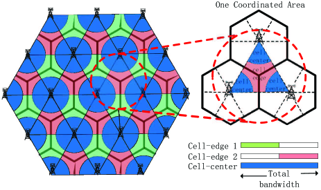
Figure 3: Implementation of the proposed transmission scheme over the general multi-cell network.

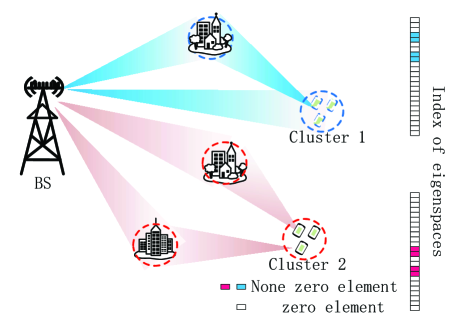
Figure 4: The scenario with multiple scattering rings.

V-C2 Beyond the one-ring model

For mathematical convenience, the one-ring scattering model is used in the previous sections. Nevertheless, the proposed scheme can be also applicable for the practical scenarios with multiple scattering rings, which is shown in Figure 4. The main differences between the one-ring and the multiple-ring models can be summarized as follows. Under the multiple-ring model, the index set $\mathcal{I}_{j}^{i}$ is a composition of multiple contiguous sequences, while that for the single-ring is just one contiguous sequences.

V-C3 Implementation in TDD system

The proposed transmission scheme is proposed to reduce the overhead for the CSI acquiring in the FDD system. Nonetheless, the proposed scheme can be directly utilized for the TDD system without changing any components. Moreover, the proposed scheme can also gain advantage in the TDD system, such as improving the performance of the cell-edge clusters.

For completeness, the detailed IA-SSR based cooperative transmission scheme is outlined in Algorithm 2.

Algorithm 2 IA-SSR based Cooperative Transmission Scheme for the Multi-cell Massive MIMO system

1:  Initialize $\mathcal{E}=\emptyset$, $\mathcal{C}_{i}=\emptyset$.

2:  for $j=1:J$ do

3:     Calculate $\mathbf{B}^{i}_{j}$ for cluster $j$ by (12).

4:     Solve problem (P1).

5:     if $\alpha_{{}_{j\in\mathcal{E}}}(S^{1}_{j}\!\!+\!\!S^{2}_{j}\!\!+\!\!S^{3}_{j})>\max(\!\alpha_{{}_{j\in\!\mathcal{C}_{1}}}\!M^{1}_{j}\!,\alpha_{{}_{j\in\!\mathcal{C}_{2}}}\!M^{2}_{j},\!\alpha_{{}_{j\in\!\mathcal{C}_{3}}}\!M^{3}_{j})$ then

6:        $\mathcal{E}=\mathcal{E}\cup\{j\}$

7:     else

8:        $i=\arg\max_{i}(\alpha_{{}_{j\in\mathcal{C}_{i}}}{M^{i}_{j}}),\mathcal{C}_{i}=\mathcal{C}_{i}\cup\{j\}$

9:     end if

10:  end for

11:  Recalculate $\{\mathbf{B}^{i}_{j}\}$ for clusters in $\mathcal{C}_{i}$ by (31).

12:  Design training matrices $\{\mathbf{T_{e}}_{j}^{i}\}$ and $\{\mathbf{T_{c}}_{j}^{i}\}$ with (50)-(53). Estimate the effective equivalent channels $\{\mathbf{H}_{j}^{i}\}$ and the channel covariances $\{\mathbf{K}_{j}\}$ with (57),(58) and (60).

13:   Calculate the inner precoder $\mathbf{V}_{j}^{i}$ for the cell-center cluster with (34).

14:   Calculate the inner precoder $\mathbf{V}_{j}^{i}$ for the cell-edge cluster by solving the equations set (19)-(21).

15:  Calculate the decoding matrix $\mathbf{U}_{j,i}$ for the cell-edge cluster through (22).

16:  Perform the power allocation through Algorithm 1.

17:  Implement thedownlink data transmission with two-stage precoder $\mathbf{P}_{j}^{i}=\mathbf{B}_{j}^{i}\mathbf{V}_{j}^{i}$.

VI Numerical Results and Discussion

In this section, we evaluate the proposed IA-SSR based cooperative transmission scheme through numerical simulations. We consider a three-cell cellular system with 2 clusters in each cell-center area and 3 clusters in the cell-edge area. The number of users in each cluster is $3$. The radius of the cell is 1 kilometer. The distance between cell-center clusters and BS is 350 meters and the distance between cell-edge clusters and BS is 900 meters. Each BS possesses $N_{t}=128$ antennas, and each user has $N_{r}=2$ antennas. The BS antenna element spacing is equal to the half wavelength. The carrier frequency is 2GHz. We generate the massive MIMO channel according to (3) and (5). The free-space path loss (FSPL) is considered. The variance of the noise is 1, and the signal-to-noise ratio (SNR) is defined as SNR $=\beta_{j\in\mathcal{C}_{i}}^{i}{P_{total}}$, which is the total transmit power normalized by the path loss of cell-center clusters. The performance of the proposed IA-SSR scheme is compared with the directly extended two-stage precoding scheme (DE scheme) for multi-cell massive MIMO network in [18] and the CoMP scheme with full CSIT in [15].

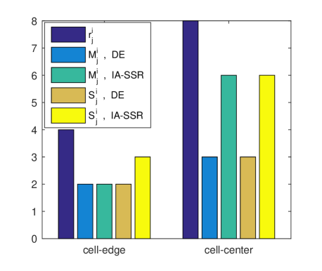
Figure 5: Comparison of the rank of channel covariance matrix, the rank of effective equivalent channel, and number of data streams in IA-SSR scheme and that in DE scheme.

Figure 5 shows the rank of the spatial correlation matrix $r_{j}^{i}$, the rank of the effective equivalent channel $M_{j}^{i}$, and the number of data streams $S_{j}^{i}$ of both DE and IA-SSR schemes, respectively. In DE scheme, we get $M_{j\in\mathcal{E}}^{i}=2$ and $M_{j\in\mathcal{C}_{i}}^{i}=3$ , which are much smaller than $r_{j\in\mathcal{E}}^{i}=4$ and $r_{j\in\mathcal{C}_{i}}^{i}=8$ due to the AoD range overlap. In this case, $S_{j\in\mathcal{E}}^{i}=2$ is smaller than the user number. As a result, one user is blocked. Whereas, $M_{j\in\mathcal{C}_{i}}^{i}=6$ in IA-SSR, which doubles that in DE scheme. The $M_{j\in\mathcal{E}}^{i}$ remains unimproved in IA-SSR, which agrees with Remark 3. But IA improves the number $S_{j\in\mathcal{E}}^{i}$ of data streams for the cell-edge cluster to 3, which is $3/2$ times of that of DE scheme.

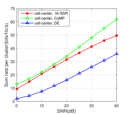
Figure 6: Sum-rate per cell-center cluster in IA-SSR scheme, DE scheme and CoMP scheme.

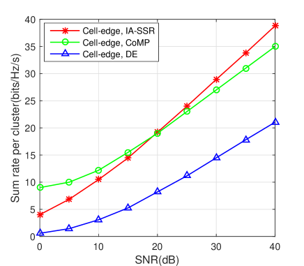
Figure 7: Sum-rate per cell-edge cluster in IA-SSR scheme, DE scheme and CoMP scheme.

Figure 6/Figure 7 compares the sum-rate per cell-center/cell-edge cluster of IA-SSR scheme against that of DE scheme and CoMP scheme. The simulation results show that the sum-rate of both the cell-center and cell-edge cluster in IA-SSR scheme is obviously higher than that of DE scheme. The sum-rate of the cell-edge cluster is almost doubled. Whereas, the improvement for the cell-center cluster is not that significant. This phenomenon may look strange as the number of data streams for the cell-center cluster is doubled, while that for the cell-edge cluster increases $3/2$ times. It can be explained as follows: in IA-SSR scheme, the transmission power for the cell-center cluster is limited to avoid interference between different cell-centers. We can also see that the performance of the proposed IA-SSR scheme is close to that of CoMP scheme with full CSIT. In high SNR regime, the sum-rate of cell-edge cluster in the IA-SSR scheme is even a little higher than that of CoMP scheme as IA provides more spatial DoF.

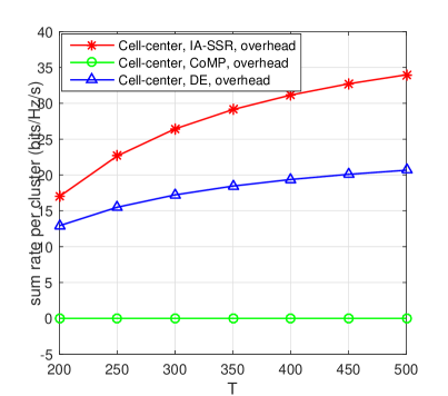
Figure 8: Effective sum-rate per cell-center cluster versus channel coherent block length $T$ (SNR = 30dB, $F=4,Q=16$).

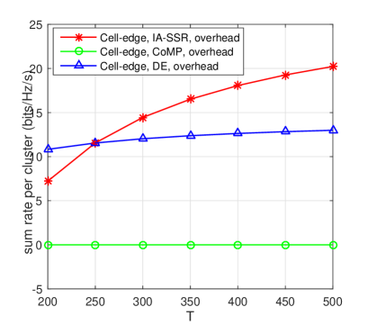
Figure 9: Effective sum-rate per cell-edge cluster versus channel coherent block length $T$ (SNR = 30dB, $F=4,Q=16$).

To uncover the overhead of our designed channel training scheme and CSI feedback, we present a numerical example of effective sum-rate in Figure 8 and Figure 9. The effective sum-rate of the IA-SSR scheme is computed according to (61), where SNR = 30dB, $F=4$ and $Q=16$ . The effective sum-rate of the DE scheme and CoMP scheme is computed in a similar approach. From Figure 8 and Figure 9, we can observe that the performance gap between IA-SSR scheme and DE scheme decreases as $T$ decreases. The sum-rate of cell-center cluster in IA-SSR scheme is always higher than that in DE scheme. Whereas, the sum-rate of the cell-edge cluster in IA-SSR scheme becomes lower than that in DE scheme when $T$ is small. The reason behind this is that the amount of needed cell-edge clusters’ CSI for IA is 3 times of that for DE scheme. We can also see that the effective sum-rate of CoMP scheme in considered $T$ is zero, due to the fact that in FDD mode all the channel resource is used for pilot transmission and full CSI feedback. Such that the CoMP scheme is only suited for TDD mode.

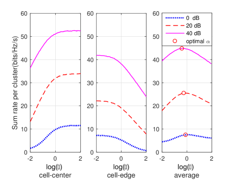
Figure 10: Sum-rate per cluster of cell-center cluster, cell-edge cluster, and their average versus $\log_{10}(\alpha)$ at SNR = 0dB, SNR = 20dB, and SNR = 40dB.

In order to evaluate the proposed power allocation policy, we define the power splitting factor as

$$\alpha=\frac{p_{cent}}{p_{edge}},$$

where $p_{edge}$ is the average power allocated to each data stream for cell-edge cluster. Figure 10 presents the sum-rate per cell-center cluster, the sum-rate per cell-edge cluster, and their average versus the power splitting factor $\alpha$ (in $\log$ form), respectively. Three different SNRs, i.e., 0 dB, 20 dB, and 40 dB are adopted here. Figure 10 shows the same results with that we analyzed in section III.C. In small $\alpha$ regimes, the sum-rate of the cell-center cluster increases significantly as $\alpha$ grows, which results in an increase of the average sum-rate. Whereas, in large $\alpha$ regimes, the sum-rate increase of the cell-center cluster is not obvious, but the sum-rate of the cell-edge cluster decreases seriously. As a result, the average sum-rate decreases. Furthermore, the optimal $\alpha$ (marked by red circle) obtained by our designed Algorithm 1 perfectly matches the peak point of average sum-rate of simulation, which verifies the efficiency our power allocation algorithm. We can also see that the optimal $\alpha$ is always smaller than 1. It means that the power of cell-center cluster is limited within a lower level than that of cell-edge cluster. By comparing the optimal $\alpha$ of three different SNRs, we realize that the optimal $\alpha$ decreases with the increase of SNR. The reason lies behind this is the interference dominates the interference plus noise at a high SNR regime, which makes the sum-rate of cell-center cluster is sensitive to interference. Therefore, the power for the cell-center cluster should be limited more strictly to avoid interference between different cell-centers at high SNR.

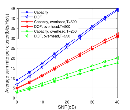
Figure 11: Comparison of the proposed effective DoF maximizing cluster division criterion and the capacity maximizing criterion.

Figure 11 compares the achievable sum rate of the effective DoF maximizing criterion with that of the achievable capacity maximizing criterion. In this example, three clusters are randomly distributed in each cell. From Figure 11, we observe that, if the overhead of CSI acquiring is ignored, the effective DoF maximizing criterion results in a slight performance loss in the low and middle SNR regimes. However, if the overhead is considered, the effective sum-rate for the effective DoF maximizing criterion is higher than that of the capacity maximizing criterion, especially under the scenario with small coherent time.

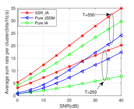
Figure 12: A performance comparison of the proposed IA-SSR scheme, the pure JSDM scheme and pure IA scheme.

In order to better appreciate the gains of the proposed IA-SSR scheme, the effective sum-rate of the proposed IA-SSR scheme is compared with those of the pure JSDM scheme and the pure IA scheme in Figure 12. The channel coherent block length $T$ is set as 250 and 550, respectively. The results show that the sum-rate of the pure JSDM scheme is higher than that of the pure IA scheme when $T$ is small. Contrarily, the pure IA scheme achieves better performance when $T$ is large. The reason behind this is that the IA scheme provides greater DoF than the JSDM scheme, but it consumes more time blocks to obtain global CSI. Since the proposed IA-SSR scheme adaptively makes a tradeoff between the IA scheme and the JSDM scheme, it always outperforms the pure IA scheme and the pure SSR scheme.

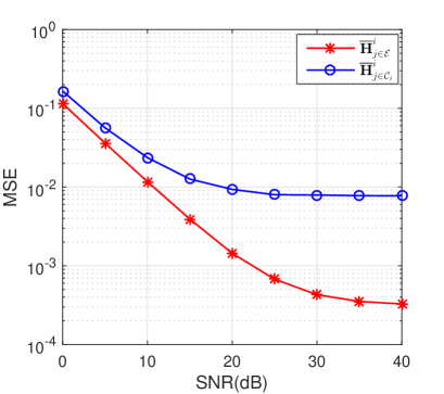
Figure 13: MSE performance of the proposed the channel training scheme.

Figure 13 evaluates the performance of our proposed channel estimation scheme in terms of MSEs. It can be seen that the MSE for the cell-center clusters is higher than that of the cell-edge clusters. The reason behind this is the cell-center clusters suffer the interference from the other cell-center areas. With the SNR increasing, the MSEs for both the cell-center clusters and the cell-edge clusters have error floors. This phenomenon can be explained as follows. The complete orthogonality of channels for different users is impossible and the slight inter-cluster interference may arise when the practical number of antennas at BS are considered.

VII Conclusions

In this paper, we investigated the two-stage precoding for the multi-cell massive MIMO systems, where multi-antennas at user side was considered. First, we proposed an IA-SSR based cooperative transmission scheme to efficiently apply the two-stage precoding for the multi-cell scenario. Then, the optimal power allocation and the low overhead channel training framework were developed for the IA-SSR scheme. Finally, the numerical simulation results showed that the proposed IA-SSR scheme yields significant performance gain over the existing methods.

References

• [1] F. Rusek, D. Persson, B. K. Lau, E. G. Larsson, T. L. Marzetta, O. Edfors, and F. Tufvesson, “Scaling up MIMO: Opportunities and challenges with very large arrays,” IEEE Signal Process. Mag., vol. 30, no. 1, pp. 40–60, Jan. 2013.
• [2] V. Jungnickel, K. Manolakis, W. Zirwas, B. Panzner, V. Braun, M. Lossow, M. Sternad, R. Apelfrojd, and T. Svensson, “The role of small cells, coordinated multipoint, and massive MIMO in 5G,” IEEE Commun. Mag., vol. 52, no. 5, pp. 44–51, May 2014.
• [3] F. Boccardi, R. W. Heath, A. Lozano, T. L. Marzetta, and P. Popovski, “Five disruptive technology directions for 5G,” IEEE Commun. Mag., vol. 52, no. 2, pp. 74–80, Feb. 2014.
• [4] J. Hoydis, S. Ten Brink, and M. Debbah, “Massive MIMO in the UL/DL of cellular networks: How many antennas do we need?” IEEE J. Sel. Areas Commun., vol. 31, no. 2, pp. 160–171, Feb. 2013.
• [5] N. Jindal, “MIMO broadcast channels with finite-rate feedback,” IEEE Trans. Inf. Theory, vol. 52, no. 11, pp. 5045–5060, Nov. 2006.
• [6] J. Choi, D. J. Love, and P. Bidigare, “Downlink training techniques for FDD massive MIMO systems: Open-loop and closed-loop training with memory,” IEEE J. Sel. Topics Signal Process., vol. 8, no. 5, pp. 802–814, Oct. 2014.
• [7] S. Noh, M. D. Zoltowski, and D. J. Love, “Training sequence design for feedback assisted hybrid beamforming in massive MIMO systems,” IEEE Trans. Commun., vol. 64, no. 1, pp. 187–200, Jan. 2016.
• [8] A. Adhikary, J. Nam, J.-Y. Ahn, and G. Caire, “Joint spatial division and multiplexing the large-scale array regime,” IEEE Trans. Inf. Theory, vol. 59, no. 10, pp. 6441–6463, Oct. 2013.
• [9] J. Nam, A. Adhikary, J. Y. Ahn, and G. Caire, “Joint spatial division and multiplexing: Opportunistic beamforming, user grouping and simplified downlink scheduling,” IEEE J. Sel. Topics Signal Process., vol. 8, no. 5, pp. 876–890, Oct. 2014.
• [10] A. Adhikary, E. A. Safadi, M. K. Samimi, R. Wang, G. Caire, T. S. Rappaport, and A. F. Molisch, “Joint spatial division and multiplexing for mm-Wave channels,” IEEE J. Sel. Areas Commun., vol. 32, no. 6, pp. 1239–1255, Jun. 2014.
• [11] A. Liu and V. Lau, “Phase only RF precoding for massive MIMO systems with limited RF chains,” IEEE Trans. Signal Process., vol. 62, no. 17, pp. 4505–4515, Sept. 2014.
• [12] D. Kim, G. Lee, and Y. Sung, “Two-stage beamformer design for massive MIMO downlink by trace quotient formulation,” IEEE Trans. Commun., vol. 63, no. 6, pp. 2200–2211, Jun. 2015.
• [13] J. Chen and V. K. N. Lau, “Two-tier precoding for FDD multi-cell massive MIMO time-varying interference networks,” IEEE J. Sel. Areas Commun., vol. 32, no. 6, pp. 1230–1238, Jun. 2014.
• [14] C. Sun, X. Gao, S. Jin, M. Matthaiou, Z. Ding, and C. Xiao, “Beam division multiple access transmission for massive MIMO communications,” IEEE Trans. Commun., vol. 63, no. 6, pp. 2170–2184, Jun. 2015.
• [15] O. Somekh, O. Simeone, Y. Bar-Ness, A. M. Haimovich and S. Shamai, “Cooperative multicell zero-forcing beamforming in cellular downlink channels,” IEEE Trans. Inf. Theory, vol. 55, no. 7, pp. 3206–3219, July 2009.
• [16] V. R. Cadambe and S. A. Jafar, “Interference alignment and degrees of freedom of the-user interference channel,” IEEE Trans. Inf. Theory, vol. 54, no. 8, pp. 3425–3441, Aug. 2008.
• [17] N. Zhao, F. R. Yu, M. Jin, Q. Yan, and V. C. M. Leung, “Interference alignment and its applications: A survey, research issues and challenges,” IEEE Commun. Surveys Tuts., to appear.
• [18] M. Kurras, L. Thiele and G. Caire, “Multi-stage beamforming for interference coordination in massive MIMO networks,” in Proc. 2015 49th Asilomar Conference on Signals, Systems and Computers, Pacific Grove, CA, pp. 700–703, 2015.
• [19] A. Adhikary and G. Caire, “JSDM and multi-cell networks: Handling inter-cell interference through long-term antenna statistics,” in Proc. 2014 48th Asilomar Conference on Signals, Systems and Computers, Pacific Grove, CA, pp. 649–655, 2014.
• [20] A. Liu and V. K. N. Lau, “Two-stage subspace constrained precoding in massive MIMO cellular systems,” IEEE Trans. on Wireless Commun., vol. 14, no. 6, pp. 3271–3279, June 2015.
• [21] L.-C. Wang and K. K. Leung, “A high-capacity wireless network by quad-sector cell and interleaved channel assignment,” IEEE J. Sel. Areas Commun., vol. 18, no. 3, pp. 472–480, Mar. 2000.
• [22] A. Abdi and M. Kaveh, “A space-time correlation model for multielement antenna systems in mobile fading channels,” IEEE J. Sel. Areas Commun., vol. 20, no. 3, pp. 550–560, Apr. 2002.
• [23] M. Zhang, P. Smith, and M. Shafi, “An extended one-ring MIMO channel model,” IEEE Trans. Wireless Commun., vol. 6, no. 8, pp. 2759–2764, Aug. 2007.
• [24] A. Forenza, D. J. Love and R. W. Heath, “Simplified Spatial Correlation Models for Clustered MIMO Channels With Different Array Configurations,” IEEE Trans. Veh. Technol., vol. 56, no. 4, pp. 1924–1934, Jul. 2007.
• [25] H. Xie, F. Gao, S. Zhang, S. Jin, “A unified transmission strategy for TDD/FDD massive MIMO systems with spatial basis expansion model,” IEEE Trans. Veh. Technol., vol. PP, no. 99, pp. 1–1, Jul. 2016.
• [26] X. Chen, C. Yuen, “On interference alignment with imperfect CSI: characteriazations of outage probability, ergodic rate and SER,” IEEE Trans. Veh. Technol., vol. 65, no. 1, pp. 47–58, Jan. 2016.
• [27] Q. Wang, D. Jiang, J. Jin, G. Liu, Z. Yan and D. Yang, “Application of BBU+RRU Based Comp System to LTE-Advanced,“ in Proc. 2009 IEEE International Conference on Communications Workshops, Dresden, 2009, pp. 1–5.
• [28] M. Sawahashi, Y. Kishiyama, A. Morimoto, D. Nishikawa and M. Tanno, “Coordinated multipoint transmission/reception techniques for LTE-advanced,” IEEE Trans. Wireless Commun., vol. 17, no. 3, pp. 26–34, June 2010.
• [29] H. Gao, T. Lv, D. Fang, S. Yang and C. Yuen, “Limited feedback-based interference alignment for interfering multi-access channels,” IEEE Commun. Lett, vol. 18, no. 4, pp. 540–543, Apr. 2014.
• [30] G. Caire and S. Shamai, “On the achievable throughput of a multiantenna Gaussian broadcast channel,” IEEE Trans. Inf. Theory, vol. 49, no. 7, pp. 1691–1706, Jul. 2003.
• [31] P. W. Baier, W. Qiu, H. Troger, C. A. Jotten, and M. Meurer, “Modelling and optimization of receiver oriented multi-user MIMO downlinks for frequency selective channels,” in Proc. 2003 Int. Conf., Telecommunications, pp. 1547–1554, Feb. 2003.
• [32] D. Tse and P. Viswanath, Fundamentals of wireless communication, Cambridge university press, 2005.
• [33] W. Sun and Y.-X. Yuan, Optimization theory and methods: nonlinear programming. Springer Science & Business Media, vol. 1, 2006.
• [34] Z. Gao, L. Dai, W. Dai, B. Shim, Z. Wang, “Structured compressive sensing-based spatio-temporal joint channel estimation for FDD massive MIMO,” IEEE Trans. Commun., vol. 64, no. 2, pp. 601–617, Feb. 2016.
• [35] H. Xie, B. Wang, F. Gao and S. Jin, ”A Full-Space Spectrum-Sharing Strategy for Massive MIMO Cognitive Radio Systems,” IEEE J. Sel. Areas Commun., vol. 34, no. 10, pp. 2537–2549, Oct. 2016.
• [36] H. Xie, F. Gao and S. Jin, ”An Overview of Low-Rank Channel Estimation for Massive MIMO Systems,” IEEE Access, vol. 4, no. , pp. 7313–7321, Nov. 2016.
• [37] W. Xu, X. Wu, X. Dong, H. Zhang, X. You, “Dual-polarized massive MIMO systems under multi-Cell pilot contamination,” IEEE Access, vol. 4, pp. 5998–6013, Sept. 2016.