On M-ary Distributed Detection for Power Constraint Wireless Sensor Networks

Zahra Hajibabaei, Jalil Modares, , Azadeh Vosoughi Z. Hajibabaei and J. Modares are with the EE Department, University at Buffalo, Buffalo, NY, e-mail: zahrahaj@buffalo.edu, jmod@buffalo.edu.A. Vosoughi is with the EECS Department, University of Central Florida, Orlando, FL, e-mail:azadeh@ucf.edu.
Abstract

We consider a wireless sensor network (WSN), consisting of several sensors and a fusion center (FC), which is tasked with solving an M-ary hypothesis testing problem. Sensors make M-ary decisions and transmit their digitally modulated decisions over orthogonal channels, which are subject to Rayleigh fading and noise, to the FC. Adopting Bayesian optimality criterion, we consider training and non-training based distributed detection systems and investigate the effect of imperfect channel state information (CSI) on the optimal maximum a posteriori probability (MAP) fusion rules and optimal power allocation between sensors, when the sum of training and data symbol transmit powers is fixed. We consider J-divergence criteria to do power allocation between sensors. The theoretical results show that J-divergence for coherent reception will be maximized if total training power be half of total power, however for non coherent reception, optimal training power which maximize J-divergence is zero. The simulated results also show that probability of error will be minimized if training power be half of total power for coherent reception and zero for non coherent reception.

Index Terms:
M-ary distributed detection, Wireless sensor networks, Power allocation, Channel estimation, Coherent and non coherent reception.

I Introduction

We consider a wireless sensor network (WSN), consisting a set of spatially distributed sensors and a fusion center (FC), that is tasked with solving an M𝑀M-ary distributed detection problem. In particular, we consider the problem of distributed classification of M𝑀M independent Gaussian sources with identical variances and different means. Sensors make local decisions individually and transmit their digitally modulated decisions to the FC, over orthogonal fading channels. The FC is tasked with fusing all the received signals from the sensors directly, via applying the optimal fusion rule, and making the final decision.
Channel-aware binary distributed detection for fusion of binary decisions transmitted over fading channels was first discussed in [1], where the FC fuses the received signals from the sensors directly (without demodulating the transmitted symbols). They considered different schemes to improve detection performance in distributed detction systems. In [2], massive MIMO has been investigated in WSN’s for coherent channel. In [3], They consider a censoring sensor network scheme and show that by adding artificial noise, the system performs very closely to the exact copula-based GLRT. In [4], they showed that using only one transmission, the detection error can be made as small as desired. In [5], they considered the problem of designing binary sensor quantizers that maximize the Kullback-Leibler (KL) divergence at the fusion center (FC) The works on channel-aware binary distributed detection are mainly built on the assumption that perfect knowledge of phase or amplitude of the fading channel coefficients are available at the FC [6, 7]. Today’s wireless communication systems with coherent reception rely upon training in order to facilitate channel estimation at the receiver. In fact, quantifying the effect of imperfect channel state information (CSI) and channel estimation error on the design and performance of wireless communication systems is a challenging problem, that has attracted the attention of researchers over the past decade [8]. Recently, channel-aware binary distributed detection with imperfect CSI was studied in [9, 10, 11].In [11], when sensors amplify and forward their observation, the performance of system under different knowledge of channel has been investigated. Sensors can send their information to the FC over Multiaccess channels or parallel access channels. In [12], the performance of system MAC Vs PAC for Non coherent reception has been studied. in [13], the performance of system when channel is non coherent has been investigated and it has been shown on-off keying scheme is the most energy efficient modulation scheme when the channel is subject to Rayleigh fading. In [14], the optimality of the received energy test in scenarios with correlated sensor decisions and non identical sensors has been verified. In [15], they proposed cooperative fusion architecture which enhance detection performance. All of these works are for the case that we have just two hypotheses and the FC should make decision between two hypotheses. channel-aware M𝑀M-ary distributed detection when the communication channels are modeled as additive white Gaussian noise (AWGN) [16] and Rayleigh fading with perfect CSI available at the FC has been studied in [16, 17, 18]. In [17] the impact of imperfect CSI on the design and performance of channel-aware M𝑀M-ary distributed detection systems has been investigated.
Due to limitation of power in WSN’s, it has been attempted to improve the performance of system by optimal power allocation between sensors. In [19], Sensors share the quantized data of their observation and it has been shown power consumption is 50 percent less than unquantized conventional methods. In [20], sensors transmit different linear combinations of their measurements through a multiple access channel (MAC) to FC and show their scheme save energy in the low signal-to-noise ratio regime. In [21], Sensors are selected based on satisfying the average global probability of detection and minimizing the energy consumption. In [6], the power allocation between sensors for binary hypotheses and known channel fading coefficients based on cost function J divergence has been done. In [22], power allocation based on maximization of deflection coefficient for partial coherent and channel statistic has been done. In [23], local power control strategy for multi-hypotheses has been introduced.The works on power allocation in distributed detection are mainly built on the assumption that perfect knowledge of the fading channel coefficients are available at the FC and power allocation for channel estimation has not been considered.In [25] power allocation for data and training of distributed estimation has been studied. In [25] power allocation of data and training of distributed estimation of a source when sensors amplify and forward their observation over MAC. In [26], power allocation between sensors when sensors amplify and forward their spatially corrolated date to FC when we have perfect channel or estimation of channel gain. To the best of our knowledge, there is no work in distributed detection for power allocation of data and training between sensors. In order to do power allocation between sensors, we need a cost function. Deriving probability of error at the FC is hard even for the case when we know complete information about the amplitude and phase of channel. We choose J divergence as our optimality criterion. [23] established a lower bound on pairwise sum of the individual error probabilities between two hypotheses, where the lower bound is a constant (determined by the a priori probabilities of the hypotheses) minus Jtotsubscript𝐽𝑡𝑜𝑡J_{tot}. Hence, by maximizing Jtotsubscript𝐽𝑡𝑜𝑡J_{tot} we minimize the lower bound on the error probability.”

In this work, we address the following questions: how should the power allocated between sensors to improve performance? how can we mitigate the negative impact of channel estimation error via optimizing transmit power allocation between data and training symbols? how do the answers to the above questions change as the reception mode at the FC and modulation scheme at the sensors vary? For non coherent reception, how does the power allocation differ for training and non-training based systems, where the sensors do not transmit training symbols (for estimating channel amplitudes) and the FC only relies on the knowledge of the channel statistics? To answer these questions we consider the following three cases, assuming Rayleigh block fading channel model: (i𝑖i) the FC is equipped with a coherent receiver and a training based channel estimator, sensors employ M𝑀M-PSK modulation for transmitting their data and training symbols, (ii𝑖𝑖ii) the FC is equipped with a non coherent receiver and a training based channel amplitude estimator, the sensors employ M𝑀M-FSK modulation for transmitting their data and training symbols, (iii𝑖𝑖𝑖iii) the FC is equipped with a non coherent receiver without a channel estimator (the FC only has the channel statistics), the sensors employ M𝑀M-FSK modulation for transmitting their data symbols. The organization of the paper follows: Section II introduces the system model. Sections III and IV derive the optimal power allocation for cases (i𝑖i),(ii𝑖𝑖ii),(iii𝑖𝑖𝑖iii) explained above. Section V includes our numerical results. Section VI concludes the paper.

II System Model and Problem Statement

We consider the problem of testing which of the M2𝑀2M\geq 2 hypotheses {m}m=1Msuperscriptsubscriptsubscript𝑚𝑚1𝑀\left\{\mathcal{H}_{m}\right\}_{m=1}^{M} has been occurred, assuming πmsubscript𝜋𝑚\pi_{m} is the a priori probability that hypothesis msubscript𝑚\mathcal{H}_{m} occurs. Our system model consists of a FC and N𝑁N spatially distributed sensors, which is tasked with solving this M𝑀M-ary hypothesis testing problem. Let 𝒙ksubscript𝒙𝑘\boldsymbol{x}_{k} denote the local observation at sensor k𝑘k during an observation period. We assume that 𝒙ksubscript𝒙𝑘\boldsymbol{x}_{k}’s are independent across sensors, conditioned on a particular hypothesis, i.e., f(𝒙1,𝒙2,,𝒙N|m)=k=1Nf(𝒙k|m)𝑓subscript𝒙1subscript𝒙2conditionalsubscript𝒙𝑁subscript𝑚superscriptsubscriptproduct𝑘1𝑁𝑓conditionalsubscript𝒙𝑘subscript𝑚f(\boldsymbol{x}_{1},\boldsymbol{x}_{2},...,\boldsymbol{x}_{N}|\mathcal{H}_{m})=\prod_{k=1}^{N}f(\boldsymbol{x}_{k}|\mathcal{H}_{m}) for m=1,,M𝑚1𝑀m=1,...,M, where f(.)f(.) denotes the probability density function (pdf). Suppose 𝒙ksubscript𝒙𝑘\boldsymbol{x}_{k} at sensor k𝑘k under hypothesis msubscript𝑚\mathcal{H}_{m} is:

m:𝒙k=𝒛mk+𝝂k,m=1,,M,k=1,,N,:subscript𝑚formulae-sequencesubscript𝒙𝑘superscriptsubscript𝒛𝑚𝑘subscript𝝂𝑘formulae-sequence𝑚1𝑀𝑘1𝑁\mathcal{H}_{m}:\boldsymbol{x}_{k}=\boldsymbol{z}_{m}^{k}+\boldsymbol{\nu}_{k},~{}~{}~{}~{}m=1,...,M,k=1,...,N, (1)

where 𝒛mksubscriptsuperscript𝒛𝑘𝑚\boldsymbol{z}^{k}_{m}’s are Gaussian signal sources with different means and equal variances, i.e., 𝒛mkN(ηmk,σz2)similar-tosuperscriptsubscript𝒛𝑚𝑘𝑁superscriptsubscript𝜂𝑚𝑘superscriptsubscript𝜎𝑧2\boldsymbol{z}_{m}^{k}\!\sim\!N(\eta_{m}^{k},\sigma_{z}^{2}), 𝝂ksubscript𝝂𝑘\boldsymbol{\nu}_{k}’s are Gaussian measurement noises 𝝂kN(0,σν2)similar-tosubscript𝝂𝑘𝑁0superscriptsubscript𝜎𝜈2\boldsymbol{\nu}_{k}\sim N(0,\sigma_{\nu}^{2}), and 𝒛mk,𝝂ksuperscriptsubscript𝒛𝑚𝑘subscript𝝂𝑘\boldsymbol{z}_{m}^{k},\boldsymbol{\nu}_{k} are all mutually uncorrelated. Each sensor applies a local rule to decide which of the M𝑀M hypotheses has occurred, such that the error probability at the sensor is minimized, i.e., the local detector of sensor k𝑘k finds lk=argminm|𝒙kηmk|subscript𝑙𝑘subscript𝑚subscript𝒙𝑘superscriptsubscript𝜂𝑚𝑘l_{k}=\arg\min_{m}|\boldsymbol{x}_{k}-\eta_{m}^{k}| and decides hypothesis ksubscript𝑘\mathcal{H}_{k}. Let pimksuperscriptsubscript𝑝𝑖𝑚𝑘p_{im}^{k} denote the probability that sensor k𝑘k decides on isubscript𝑖\mathcal{H}_{i}, given that the true hypothesis is msubscript𝑚\mathcal{H}_{m}. For the sensing model in (1), one can verify that pimksuperscriptsubscript𝑝𝑖𝑚𝑘p_{im}^{k} is:

pimk={Q(ηik+ηi1k2ηmk2(σν2+σz2))Q(ηik+ηi+1k2ηmk2(σν2+σz2))i1,M1Q(η1k+η2k2ηmk2(σν2+σz2))i=1Q(ηMk+ηM1k2ηmk2(σν2+σz2))i=Msuperscriptsubscript𝑝𝑖𝑚𝑘cases𝑄superscriptsubscript𝜂𝑖𝑘subscriptsuperscript𝜂𝑘𝑖12subscriptsuperscript𝜂𝑘𝑚2superscriptsubscript𝜎𝜈2superscriptsubscript𝜎𝑧2𝑄superscriptsubscript𝜂𝑖𝑘subscriptsuperscript𝜂𝑘𝑖12subscriptsuperscript𝜂𝑘𝑚2superscriptsubscript𝜎𝜈2superscriptsubscript𝜎𝑧2𝑖1𝑀1𝑄superscriptsubscript𝜂1𝑘subscriptsuperscript𝜂𝑘22subscriptsuperscript𝜂𝑘𝑚2superscriptsubscript𝜎𝜈2superscriptsubscript𝜎𝑧2𝑖1𝑄subscriptsuperscript𝜂𝑘𝑀subscriptsuperscript𝜂𝑘𝑀12subscriptsuperscript𝜂𝑘𝑚2superscriptsubscript𝜎𝜈2superscriptsubscript𝜎𝑧2𝑖𝑀\displaystyle p_{im}^{k}=\begin{cases}Q(\frac{\eta_{i}^{k}+\eta^{k}_{i-1}-2\eta^{k}_{m}}{2(\sigma_{\nu}^{2}+\sigma_{z}^{2})})-Q(\frac{\eta_{i}^{k}+\eta^{k}_{i+1}-2\eta^{k}_{m}}{2(\sigma_{\nu}^{2}+\sigma_{z}^{2})})&i\neq 1,M\\ 1-Q(\frac{\eta_{1}^{k}+\eta^{k}_{2}-2\eta^{k}_{m}}{2(\sigma_{\nu}^{2}+\sigma_{z}^{2})})&i=1\\ Q(\frac{\eta^{k}_{M}+\eta^{k}_{M-1}-2\eta^{k}_{m}}{2(\sigma_{\nu}^{2}+\sigma_{z}^{2})})&i=M\end{cases} (2)

where the Q𝑄Q-function is defined as Q(x)=12πxet2/2𝑑t𝑄𝑥12𝜋superscriptsubscript𝑥superscript𝑒superscript𝑡22differential-d𝑡Q(x)=\frac{1}{\sqrt{2\pi}}\int_{x}^{\infty}e^{-t^{2}/2}dt. Sensor k𝑘k employs an M𝑀M-ary digital modulator to map its M𝑀M-ary decision to a symbol and transmits this symbol with power Pdksubscript𝑃𝑑𝑘P_{dk}. We consider M𝑀M-PSK and M𝑀M-FSK modulation at the sensors. Let 𝒖ksubscript𝒖𝑘\boldsymbol{u}_{k} and 𝒖¯ksubscript¯𝒖𝑘\underline{\boldsymbol{u}}_{k} denote the modulated symbol at sensor k𝑘k corresponding to M𝑀M-PSK and M𝑀M-FSK modulation, respectively, where scalar 𝒖k{ej2πi1M,i=1,,M}\boldsymbol{u}_{k}\in\{e^{j2\pi\frac{i-1}{M}},i=1,...,M\}, M×1𝑀1M\times 1 vector 𝒖¯k{e¯i,i=1,,M}\underline{\boldsymbol{u}}_{k}\in\{\underline{e}_{i},i=1,...,M\} and e¯isubscript¯𝑒𝑖\underline{e}_{i} is an M×1𝑀1M\times 1 canonical vector whose all elements except the i𝑖i-th one are zeros. We refer to the modulated symbols 𝒖ksubscript𝒖𝑘\boldsymbol{u}_{k}, 𝒖¯ksubscript¯𝒖𝑘\underline{\boldsymbol{u}}_{k} as data symbols and Pdksubscript𝑃𝑑𝑘P_{dk} as data symbol transmit power corresponding to sensor k𝑘k. Assuming the data symbols are sent over orthogonal channels between sensors and the FC, we represent the channel output at the FC upon the reception of data symbols as a N×1𝑁1N\times 1 vector 𝒚¯d=[𝒚d1;;𝒚dk;;𝒚dN]subscript¯𝒚𝑑subscript𝒚𝑑1subscript𝒚𝑑𝑘subscript𝒚𝑑𝑁\underline{\boldsymbol{y}}_{d}=\left[\boldsymbol{y}_{d1};...;\boldsymbol{y}_{dk};...;\boldsymbol{y}_{dN}\right] for M𝑀M-PSK modulation and MN×1𝑀𝑁1MN\times 1 𝒚¯d=[𝒚¯d1;;𝒚¯dk;;𝒚¯dN]subscript¯𝒚𝑑subscript¯𝒚𝑑1subscript¯𝒚𝑑𝑘subscript¯𝒚𝑑𝑁\underline{\boldsymbol{y}}_{d}=\left[\underline{\boldsymbol{y}}_{d1};...;\underline{\boldsymbol{y}}_{dk};...;\underline{\boldsymbol{y}}_{dN}\right] for M𝑀M-FSK modulation. In particular, the channel output corresponding to sensor k𝑘k is:

𝒚dksubscript𝒚𝑑𝑘\displaystyle\boldsymbol{y}_{dk} =Pdk𝒉k𝒖k+𝒏dk,k=1,,NM-PSK,formulae-sequenceabsentsubscript𝑃𝑑𝑘subscript𝒉𝑘subscript𝒖𝑘subscript𝒏𝑑𝑘𝑘1𝑁𝑀-PSK\displaystyle=\sqrt{P_{dk}}\boldsymbol{h}_{k}\boldsymbol{u}_{k}+\boldsymbol{n}_{dk},~{}~{}~{}~{}k=1,...,N~{}~{}M\mbox{-PSK},
𝒚¯dksubscript¯𝒚𝑑𝑘\displaystyle\underline{\boldsymbol{y}}_{dk} =Pdkhk𝒖¯k+𝒏¯dk,k=1,,NM-FSK.formulae-sequenceabsentsubscript𝑃𝑑𝑘subscript𝑘subscript¯𝒖𝑘subscript¯𝒏𝑑𝑘𝑘1𝑁𝑀-FSK\displaystyle=\sqrt{P_{dk}}{h}_{k}\underline{\boldsymbol{u}}_{k}+\underline{\boldsymbol{n}}_{dk},~{}~{}~{}~{}k=1,...,N~{}~{}M\mbox{-FSK}. (3)

The communication channel noises, denoted as scalar 𝒏dksubscript𝒏𝑑𝑘\boldsymbol{n}_{dk} and M×1𝑀1M\times 1 vector 𝒏¯dksubscript¯𝒏𝑑𝑘\underline{\boldsymbol{n}}_{dk}, are identically distributed zero mean complex Gaussian 𝒏dkCN(0,σn2)similar-tosubscript𝒏𝑑𝑘𝐶𝑁0superscriptsubscript𝜎𝑛2\boldsymbol{n}_{dk}\sim CN(0,\sigma_{n}^{2}), 𝒏¯dkCN(0,σn2I)similar-tosubscript¯𝒏𝑑𝑘𝐶𝑁0superscriptsubscript𝜎𝑛2𝐼\underline{\boldsymbol{n}}_{dk}\sim CN(0,\sigma_{n}^{2}I), where I𝐼I is an M×M𝑀𝑀M\times M identity matrix. We assume that the channel outputs conditioned on the channel inputs, are independent across the sensors. The complex channel coefficient 𝒉ksubscript𝒉𝑘\boldsymbol{h}_{k} in (II) is modeled as 𝒉kCN(0,σhk2)similar-tosubscript𝒉𝑘𝐶𝑁0subscriptsuperscript𝜎2subscript𝑘\boldsymbol{h}_{k}\sim CN(0,\sigma^{2}_{h_{k}}) where 𝒉k=αkejϕksubscript𝒉𝑘subscript𝛼𝑘superscript𝑒𝑗subscriptitalic-ϕ𝑘\boldsymbol{h}_{k}=\mathbf{\alpha}_{k}e^{j\mathbf{\phi}_{k}}, the amplitude αksubscript𝛼𝑘\mathbf{\alpha}_{k} and the phase ϕksubscriptitalic-ϕ𝑘\mathbf{\phi}_{k}, have Rayleigh and uniform distributions, respectively. To enable training based channel estimation, we assume that the channel coefficients are fixed for two consecutive symbol intervals, and each sensor sends a training symbol with power Ptksubscript𝑃𝑡𝑘P_{tk} along with its data symbol. We refer to the symbols utsubscript𝑢𝑡u_{t}, u¯tsubscript¯𝑢𝑡\underline{u}_{t} as training symbols and Ptksubscript𝑃𝑡𝑘P_{tk} as training symbol transmit power corresponding to sensor k𝑘k. Without loss of generality, we assume ut=1subscript𝑢𝑡1u_{t}\!=\!1 and u¯t=e¯1subscript¯𝑢𝑡subscript¯𝑒1\underline{u}_{t}\!=\!\underline{e}_{1}, respectively, when the sensors employ M𝑀M-PSK and M𝑀M-FSK modulation schemes. Training symbols are also sent over orthogonal channels between sensors and the FC, prior to sending data symbols. The channel output corresponding to sensor k𝑘k at the FC upon the reception of training symbol is:

𝒚tksubscript𝒚𝑡𝑘\displaystyle\boldsymbol{y}_{tk} =Ptk𝒉kut+𝒏tk,k=1,,NM-PSK,formulae-sequenceabsentsubscript𝑃𝑡𝑘subscript𝒉𝑘subscript𝑢𝑡subscript𝒏𝑡𝑘𝑘1𝑁𝑀-PSK\displaystyle=\sqrt{P_{tk}}\boldsymbol{h}_{k}u_{t}+\boldsymbol{n}_{tk},~{}~{}~{}~{}k=1,...,N~{}~{}M\mbox{-PSK},
𝒚¯tksubscript¯𝒚𝑡𝑘\displaystyle\underline{\boldsymbol{y}}_{tk} =Ptk𝒉ku¯t+𝒏¯tk,k=1,,NM-FSK,formulae-sequenceabsentsubscript𝑃𝑡𝑘subscript𝒉𝑘subscript¯𝑢𝑡subscript¯𝒏𝑡𝑘𝑘1𝑁𝑀-FSK\displaystyle=\sqrt{P_{tk}}\boldsymbol{h}_{k}\underline{u}_{t}+\underline{\boldsymbol{n}}_{tk},~{}~{}~{}~{}k=1,...,N~{}~{}M\mbox{-FSK}, (4)

where the identically distributed zero mean complex Gaussian noises 𝒏tkCN(0,σn2)similar-tosubscript𝒏𝑡𝑘𝐶𝑁0superscriptsubscript𝜎𝑛2\boldsymbol{n}_{tk}\sim CN(0,\sigma_{n}^{2}), 𝒏¯tkCN(0,σn2I)similar-tosubscript¯𝒏𝑡𝑘𝐶𝑁0superscriptsubscript𝜎𝑛2𝐼\underline{\boldsymbol{n}}_{tk}\sim CN(0,\sigma_{n}^{2}I) are independent from 𝒏dksubscript𝒏𝑑𝑘\boldsymbol{n}_{dk} and 𝒏¯dksubscript¯𝒏𝑑𝑘\underline{\boldsymbol{n}}_{dk} in (3). We consider both coherent and non-coherent receivers. The unknown channel parameters to be estimated depend on the receiver structure. For a coherent receiver with a training based channel estimator and a non-coherent receiver with a training based channel amplitude estimator, the unknown parameters are 𝒉ksubscript𝒉𝑘\boldsymbol{h}_{k} and 𝜶ksubscript𝜶𝑘\boldsymbol{\alpha}_{k}, respectively. We model these as 𝒉k=𝒉^k+𝒉~ksubscript𝒉𝑘subscriptbold-^𝒉𝑘subscriptbold-~𝒉𝑘\boldsymbol{h}_{k}=\boldsymbol{\hat{h}}_{k}+\boldsymbol{\tilde{h}}_{k} and 𝜶k=𝜶^k+𝜶~ksubscript𝜶𝑘subscriptbold-^𝜶𝑘subscriptbold-~𝜶𝑘\boldsymbol{\alpha}_{k}=\boldsymbol{\hat{\alpha}}_{k}+\boldsymbol{\tilde{\alpha}}_{k}, where 𝒉^ksubscriptbold-^𝒉𝑘\boldsymbol{\hat{h}}_{k} and 𝜶^ksubscriptbold-^𝜶𝑘\boldsymbol{\hat{\alpha}}_{k} are the estimates based on 𝒚tksubscript𝒚𝑡𝑘\boldsymbol{y}_{tk} and 𝒗tk=|𝒚tk1|2subscript𝒗𝑡𝑘superscriptsuperscriptsubscript𝒚𝑡𝑘12\boldsymbol{v}_{tk}=|\boldsymbol{y}_{tk}^{1}|^{2} in (II) respectively, and 𝒉~ksubscriptbold-~𝒉𝑘\boldsymbol{\tilde{h}}_{k} and 𝜶~ksubscriptbold-~𝜶𝑘\boldsymbol{\tilde{\alpha}}_{k} are the estimation errors111As we mentioned in Section I, the sensors employ M𝑀M-FSK modulation when the FC is equipped with a non-coherent receiver and a training based channel amplitude estimator. Since u¯t=e¯1subscript¯𝑢𝑡subscript¯𝑒1\underline{u}_{t}=\underline{e}_{1}, the estimator only employs the first entry of vector 𝒚¯tksubscript¯𝒚𝑡𝑘\underline{\boldsymbol{y}}_{tk}, denoted as 𝒚tk1superscriptsubscript𝒚𝑡𝑘1\boldsymbol{y}_{tk}^{1}, for channel amplitude estimation.. Suppose there is a constraint on the network transmit power, i.e., k=1NPkPtotsuperscriptsubscript𝑘1𝑁subscript𝑃𝑘subscript𝑃𝑡𝑜𝑡\sum_{k=1}^{N}P_{k}\leq P_{tot}, where Pk=Pdk+Ptksubscript𝑃𝑘subscript𝑃𝑑𝑘subscript𝑃𝑡𝑘P_{k}=P_{dk}+P_{tk} is total transmit power for sending data and training symbols at sensor k𝑘k. This modeling allows us to consider the energy cost of channel estimation in network power allocation. Let Pd=k=1NPdksubscript𝑃𝑑superscriptsubscript𝑘1𝑁subscript𝑃𝑑𝑘P_{d}=\sum_{k=1}^{N}P_{dk} be the total power devoted for sending all data symbols to FC and, Pt=k=1NPtksubscript𝑃𝑡superscriptsubscript𝑘1𝑁subscript𝑃𝑡𝑘P_{t}=\sum_{k=1}^{N}P_{tk} be the total power devoted for sending all training symbols to the FC. With this notation, we find Pd+PtPtotsubscript𝑃𝑑subscript𝑃𝑡subscript𝑃𝑡𝑜𝑡P_{d}+P_{t}\leq P_{tot}. We define r=Pd/Ptot𝑟subscript𝑃𝑑subscript𝑃𝑡𝑜𝑡r=P_{d}/P_{tot} as the fraction of the power assigned to all data symbols and rk=Pdk/Pksubscript𝑟𝑘subscript𝑃𝑑𝑘subscript𝑃𝑘r_{k}=P_{dk}/P_{k} for k=1,,N𝑘1𝑁k=1,...,N as the fraction of the power assigned to the data symbol at sensor k𝑘k where r,rk[0,1]𝑟subscript𝑟𝑘01r,r_{k}\in[0,1].
Our goal is to derive J-divergence in closed form expression. For M𝑀M-ary hypothesis testing, [23] defined J-divergence as weighted pairwise J-divergence between hypothesis isubscript𝑖\mathcal{H}_{i} and jsubscript𝑗\mathcal{H}_{j}, that is Jtot|𝑮^=(1/2)i=1Mj=1MπiπjJijsubscript𝐽conditional𝑡𝑜𝑡bold-^𝑮12superscriptsubscript𝑖1𝑀superscriptsubscript𝑗1𝑀subscript𝜋𝑖subscript𝜋𝑗subscript𝐽𝑖𝑗J_{tot|\boldsymbol{\hat{G}}}=(1/2)\sum_{i=1}^{M}\sum_{j=1}^{M}\pi_{i}\pi_{j}J_{ij} where Jij=J(f(𝒚¯d|i,𝑮^),f(𝒚¯d|j,𝑮^))subscript𝐽𝑖𝑗𝐽𝑓conditionalsubscriptbold-¯𝒚𝑑subscript𝑖bold-^𝑮𝑓conditionalsubscriptbold-¯𝒚𝑑subscript𝑗bold-^𝑮J_{ij}=J(f(\boldsymbol{\underline{y}}_{d}|\mathcal{H}_{i},\boldsymbol{\hat{G}}),f(\boldsymbol{\underline{y}}_{d}|\mathcal{H}_{j},\boldsymbol{\hat{G}})), where 𝑮^=diag{𝒉^1,,𝒉^N}bold-^𝑮𝑑𝑖𝑎𝑔subscriptbold-^𝒉1subscriptbold-^𝒉𝑁\boldsymbol{\hat{G}}\!=diag\{\boldsymbol{\hat{h}}_{1},...,\boldsymbol{\hat{h}}_{N}\} for coherent receiver, 𝑮^=diag{𝜶^1,,𝜶^N}bold-^𝑮𝑑𝑖𝑎𝑔subscriptbold-^𝜶1subscriptbold-^𝜶𝑁\boldsymbol{\hat{G}}\!=\!diag\left\{\boldsymbol{\hat{\alpha}}_{1},...,\boldsymbol{\hat{\alpha}}_{N}\right\} for non-coherent receiver with a training based channel amplitude estimator, and 𝑮^bold-^𝑮\boldsymbol{\hat{G}} is null for non-coherent receiver without a channel estimator, in order to incorporate the knowledge of the FC about the channel parameters, and the average J-divergence Javg=𝔼𝑮^{Jtot|𝑮^}subscript𝐽𝑎𝑣𝑔subscript𝔼bold-^𝑮subscript𝐽conditional𝑡𝑜𝑡bold-^𝑮J_{avg}=\mathbb{E}_{\boldsymbol{\hat{G}}}\{J_{tot|\boldsymbol{\hat{G}}}\}.

III Optimal fusion rules

In this section, we adopt the Bayesian criterion to find the optimal fusion rule at the FC, in order to make a global decision u0{1,2,..,M}u_{0}\in\left\{\mathcal{H}_{1},\mathcal{H}_{2},..,\mathcal{H}_{M}\right\}. The optimal fusion rule is u0=argmaxmπmΘmsubscript𝑢0subscript𝑚subscript𝜋𝑚subscriptΘ𝑚u_{0}=\arg\max_{m}\pi_{m}\Theta_{m} where ΘmsubscriptΘ𝑚\Theta_{m} varies, depending on the receiver structure and the modulation scheme. Note that the channel outputs are independent across sensors. When sensors employ M𝑀M-PSK and the receiver is coherent we find:

ΘmsubscriptΘ𝑚\displaystyle\!\!\!\!\!\!\!\!\!\Theta_{m}\!\! =\displaystyle\!\!=\!\! k=1Nf(𝒚dk|m)=k=1Ni=1Mpimkf(𝒚dk|𝒖k(i),𝑮^(k)).superscriptsubscriptproduct𝑘1𝑁𝑓conditionalsubscript𝒚𝑑𝑘subscript𝑚superscriptsubscriptproduct𝑘1𝑁superscriptsubscript𝑖1𝑀superscriptsubscript𝑝𝑖𝑚𝑘𝑓conditionalsubscript𝒚𝑑𝑘subscript𝒖𝑘𝑖bold-^𝑮𝑘\displaystyle\!\!\prod_{k=1}^{N}f(\boldsymbol{y}_{dk}|\mathcal{H}_{m})\!=\!\prod_{k=1}^{N}\sum_{i=1}^{M}p_{im}^{k}f(\boldsymbol{y}_{dk}|\boldsymbol{u}_{k}(i),\boldsymbol{\hat{G}}(k)). (5)

When sensors employ M𝑀M-FSK and the receiver is non-coherent we obtain:

ΘmsubscriptΘ𝑚\displaystyle\Theta_{m}\!\! =\displaystyle\!\!=\!\! k=1Ni=1Mpimkf(𝒚¯dk|𝒖¯k(i),𝑮^(k)),superscriptsubscriptproduct𝑘1𝑁superscriptsubscript𝑖1𝑀superscriptsubscript𝑝𝑖𝑚𝑘𝑓conditionalsubscript¯𝒚𝑑𝑘subscript¯𝒖𝑘𝑖bold-^𝑮𝑘\displaystyle\!\!\prod_{k=1}^{N}\sum_{i=1}^{M}p_{im}^{k}f(\underline{\boldsymbol{y}}_{dk}|\underline{\boldsymbol{u}}_{k}(i),\boldsymbol{\hat{G}}(k)), (6)

where 𝑮^(k)bold-^𝑮𝑘\boldsymbol{\hat{G}}(k) is the k𝑘k-th diagonal entry of 𝑮^bold-^𝑮\boldsymbol{\hat{G}}, 𝒖k(i)subscript𝒖𝑘𝑖\boldsymbol{u}_{k}(i), 𝒖¯k(i)subscript¯𝒖𝑘𝑖\underline{\boldsymbol{u}}_{k}(i) in (5), (6) are the transmitted data symbols of sensor k𝑘k corresponding to the decision of isubscript𝑖\mathcal{H}_{i} and pimksuperscriptsubscript𝑝𝑖𝑚𝑘p_{im}^{k} is obtained from (2).

III-A Coherent Reception with Imperfect CSI

For the linear signal model in (II), the minimum mean square error (MMSE) of channel estimation 𝒉ksubscript𝒉𝑘\boldsymbol{h}_{k} given 𝒚tksubscript𝒚𝑡𝑘\boldsymbol{y}_{tk} is 𝒉^k=𝔼{𝒉k|𝒚tk}=σhk2Ptkσhk2Ptk+σn2𝒚tksubscriptbold-^𝒉𝑘𝔼conditional-setsubscript𝒉𝑘subscript𝒚𝑡𝑘superscriptsubscript𝜎subscript𝑘2subscript𝑃𝑡𝑘subscriptsuperscript𝜎2subscript𝑘subscript𝑃𝑡𝑘superscriptsubscript𝜎𝑛2subscript𝒚𝑡𝑘\boldsymbol{\hat{h}}_{k}=\mathbb{E}\left\{\boldsymbol{h}_{k}|\boldsymbol{y}_{tk}\right\}=\frac{\sigma_{h_{k}}^{2}\sqrt{P_{tk}}}{\sigma^{2}_{h_{k}}P_{tk}+\sigma_{n}^{2}}\boldsymbol{y}_{tk}. Considering (4), we observe that 𝒚tkCN(0,Ptkσhk2+σn2)similar-tosubscript𝒚𝑡𝑘𝐶𝑁0subscript𝑃𝑡𝑘subscriptsuperscript𝜎2subscript𝑘subscriptsuperscript𝜎2𝑛\boldsymbol{y}_{tk}\sim CN(0,P_{tk}\sigma^{2}_{h_{k}}+\sigma^{2}_{n}). Let γtk=Ptk/σn2subscript𝛾𝑡𝑘subscript𝑃𝑡𝑘subscriptsuperscript𝜎2𝑛\gamma_{tk}=P_{tk}/\sigma^{2}_{n}. Since 𝒉^ksubscriptbold-^𝒉𝑘\boldsymbol{\hat{h}}_{k} is a linear function of 𝒚tksubscript𝒚𝑡𝑘\boldsymbol{y}_{tk}, we have 𝒉^kCN(0,σhk4γtk1+σhk2γtk)similar-tosubscriptbold-^𝒉𝑘𝐶𝑁0subscriptsuperscript𝜎4subscript𝑘subscript𝛾𝑡𝑘1subscriptsuperscript𝜎2subscript𝑘subscript𝛾𝑡𝑘\boldsymbol{\hat{h}}_{k}\sim CN(0,\frac{\sigma^{4}_{h_{k}}\gamma_{tk}}{1+\sigma^{2}_{h_{k}}\gamma_{tk}}) and 𝒉~kCN(0,σhk21+σhk2γtk)similar-tosubscriptbold-~𝒉𝑘𝐶𝑁0subscriptsuperscript𝜎2subscript𝑘1subscriptsuperscript𝜎2subscript𝑘subscript𝛾𝑡𝑘\boldsymbol{\tilde{h}}_{k}\sim CN(0,\frac{\sigma^{2}_{h_{k}}}{1+\sigma^{2}_{h_{k}}\gamma_{tk}}) [9]. To find f(𝒚dk|𝒖k(i),𝒉^k)𝑓conditionalsubscript𝒚𝑑𝑘subscript𝒖𝑘𝑖subscriptbold-^𝒉𝑘f(\boldsymbol{y}_{dk}|\boldsymbol{u}_{k}(i),\boldsymbol{\hat{h}}_{k}) in (5), we realize that given 𝒖k(i)subscript𝒖𝑘𝑖\boldsymbol{u}_{k}(i) and 𝒉^ksubscriptbold-^𝒉𝑘\boldsymbol{\hat{h}}_{k}, we have 𝒚dkCN(Pdk𝒉^k𝒖k(i),σwk2)similar-tosubscript𝒚𝑑𝑘𝐶𝑁subscript𝑃𝑑𝑘subscriptbold-^𝒉𝑘subscript𝒖𝑘𝑖subscriptsuperscript𝜎2subscript𝑤𝑘\boldsymbol{y}_{dk}\sim CN(\sqrt{P_{dk}}\boldsymbol{\hat{h}}_{k}\boldsymbol{u}_{k}(i),\sigma^{2}_{w_{k}}) where σwk2=Pdkσh~k2+σn2subscriptsuperscript𝜎2subscript𝑤𝑘subscript𝑃𝑑𝑘subscriptsuperscript𝜎2subscript~𝑘subscriptsuperscript𝜎2𝑛\sigma^{2}_{w_{k}}=P_{dk}\sigma^{2}_{{\tilde{h}}_{k}}+\sigma^{2}_{n}. Therefore, one can write the conditional pdf f(𝒚dk|𝒖k(i),𝒉^k)𝑓conditionalsubscript𝒚𝑑𝑘subscript𝒖𝑘𝑖subscriptbold-^𝒉𝑘f(\boldsymbol{y}_{dk}|\boldsymbol{u}_{k}(i),\boldsymbol{\hat{h}}_{k}) and find ΘmsubscriptΘ𝑚\Theta_{m}. After eliminating the terms that are independent of m𝑚m, the fusion rule reduces to u0=argmaxmπmΘmsubscript𝑢0subscript𝑚subscript𝜋𝑚subscriptΘ𝑚u_{0}=\arg\max_{m}\pi_{m}\Theta_{m} where ΘmsubscriptΘ𝑚\Theta_{m} is:

Θm=k=1Ni=1Mpimkexp(2PdkRe(ej2π(i1)M𝒚dk𝒉^k)σwk2).subscriptΘ𝑚superscriptsubscriptproduct𝑘1𝑁superscriptsubscript𝑖1𝑀superscriptsubscript𝑝𝑖𝑚𝑘2subscript𝑃𝑑𝑘𝑅𝑒superscript𝑒𝑗2𝜋𝑖1𝑀subscript𝒚𝑑𝑘superscriptsubscriptbold-^𝒉𝑘superscriptsubscript𝜎subscript𝑤𝑘2\!\!\!\!\Theta_{m}=\prod_{k=1}^{N}\sum_{i=1}^{M}p_{im}^{k}\exp\left(\frac{2\sqrt{P_{dk}}Re(e^{\frac{-j2\pi(i-1)}{M}}\boldsymbol{y}_{dk}\boldsymbol{\hat{h}}_{k}^{*})}{\sigma_{w_{k}}^{2}}\right). (7)

Note that the optimal fusion rule depends on Pk,rksubscript𝑃𝑘subscript𝑟𝑘P_{k},r_{k} (through Pdk,σwk2subscript𝑃𝑑𝑘superscriptsubscript𝜎subscript𝑤𝑘2P_{dk},\sigma_{w_{k}}^{2}), channel outputs 𝒚dksubscript𝒚𝑑𝑘\boldsymbol{y}_{dk}, channel estimates 𝒉^ksubscriptbold-^𝒉𝑘\boldsymbol{\hat{h}}_{k}, and local sensor performance indices pimksuperscriptsubscript𝑝𝑖𝑚𝑘p_{im}^{k}. For the special case of M=2𝑀2M\!=\!2, the optimal fusion rule reduces to:

k=1Nlog(p22k+(1p22k)e4Pdkσwk2Re(𝒚dk𝒉^k)p21k+(1p21k)e4Pdkσwk2Re(𝒚dk𝒉^k))H0H1log(π0π1).superscriptsubscript𝑘1𝑁superscriptsubscript𝑝22𝑘1superscriptsubscript𝑝22𝑘superscript𝑒4subscript𝑃𝑑𝑘subscriptsuperscript𝜎2subscript𝑤𝑘𝑅𝑒subscript𝒚𝑑𝑘superscriptsubscriptbold-^𝒉𝑘superscriptsubscript𝑝21𝑘1superscriptsubscript𝑝21𝑘superscript𝑒4subscript𝑃𝑑𝑘subscriptsuperscript𝜎2subscript𝑤𝑘𝑅𝑒subscript𝒚𝑑𝑘superscriptsubscriptbold-^𝒉𝑘subscript𝐻1subscript𝐻0greater-than-or-equals-or-less-thansubscript𝜋0subscript𝜋1\!\!\!\sum_{k=1}^{N}{\log\left(\frac{p_{22}^{k}+(1-p_{22}^{k})e^{-\frac{4\sqrt{P_{dk}}}{\sigma^{2}_{w_{k}}}Re({\boldsymbol{y}_{dk}}\boldsymbol{\hat{h}}_{k}^{*})}}{p_{21}^{k}+(1-p_{21}^{k})e^{-\frac{4\sqrt{P_{dk}}}{\sigma^{2}_{w_{k}}}Re({\boldsymbol{y}_{dk}}\boldsymbol{\hat{h}}_{k}^{*})}}\right)}\overset{H_{1}}{\underset{H_{0}}{\gtreqqless}}{\log\left(\frac{\pi_{0}}{\pi_{1}}\right)}.

III-B Non-coherent Reception with Imperfect Channel Amplitude

The MMSE estimate of the channel amplitude 𝜶ksubscript𝜶𝑘\boldsymbol{\alpha}_{k} given 𝒗tk=|𝒚tk1|2subscript𝒗𝑡𝑘superscriptsubscriptsuperscript𝒚1𝑡𝑘2\boldsymbol{v}_{tk}=|\boldsymbol{y}^{1}_{tk}|^{2} is 𝜶^k=𝔼{𝜶k|𝒗tk}=αkf(αk|𝒗tk)𝑑αksubscriptbold-^𝜶𝑘𝔼conditional-setsubscript𝜶𝑘subscript𝒗𝑡𝑘subscript𝛼𝑘𝑓conditionalsubscript𝛼𝑘subscript𝒗𝑡𝑘differential-dsubscript𝛼𝑘\boldsymbol{\hat{\alpha}}_{k}=\mathbb{E}\left\{\boldsymbol{\alpha}_{k}|\boldsymbol{v}_{tk}\right\}=\int\alpha_{k}f(\alpha_{k}|\boldsymbol{v}_{tk})d\alpha_{k}, where the conditional pdf f(𝜶k|𝒗tk)𝑓conditionalsubscript𝜶𝑘subscript𝒗𝑡𝑘f(\boldsymbol{\alpha}_{k}|\boldsymbol{v}_{tk}) is [9]:

f(𝜶k|𝒗tk)=2𝜶k(1+γtk)exp(γtk𝒗tk(1+γtk)σn2(1+γtk𝜶k2))×I0(2𝜶kγtk𝒗tkσn2),𝑓conditionalsubscript𝜶𝑘subscript𝒗𝑡𝑘2subscript𝜶𝑘1subscript𝛾𝑡𝑘subscript𝛾𝑡𝑘subscript𝒗𝑡𝑘1subscript𝛾𝑡𝑘subscriptsuperscript𝜎2𝑛1subscript𝛾𝑡𝑘subscriptsuperscript𝜶2𝑘subscript𝐼02subscript𝜶𝑘subscript𝛾𝑡𝑘subscript𝒗𝑡𝑘subscriptsuperscript𝜎2𝑛\begin{split}f(\boldsymbol{\alpha}_{k}|\boldsymbol{v}_{tk})=&2\boldsymbol{\alpha}_{k}(1+\gamma_{tk})\exp(\frac{\gamma_{tk}\boldsymbol{v}_{tk}}{(1+\gamma_{tk})\sigma^{2}_{n}}-(1+\gamma_{tk}\boldsymbol{\alpha}^{2}_{k}))\\ &\times I_{0}(2\boldsymbol{\alpha}_{k}\sqrt{\gamma_{tk}\frac{\boldsymbol{v}_{tk}}{\sigma^{2}_{n}}}),\\ \end{split}

and I0(.)I_{0}(.) is the modified Bessel functin of the first kind with order zero. Given 𝒗tksubscript𝒗𝑡𝑘\boldsymbol{v}_{tk}, we have 𝜶kRice(ν,s2)similar-tosubscript𝜶𝑘Rice𝜈superscript𝑠2\boldsymbol{\alpha}_{k}\sim\mathrm{Rice}(\nu,s^{2}) where ν=1γtk+1γtk𝒗tkσn2𝜈1subscript𝛾𝑡𝑘1subscript𝛾𝑡𝑘subscript𝒗𝑡𝑘subscriptsuperscript𝜎2𝑛\nu=\frac{1}{\gamma_{tk}+1}\sqrt{\gamma_{tk}\frac{\boldsymbol{v}_{tk}}{\sigma^{2}_{n}}} and s2=1γtk+1superscript𝑠21subscript𝛾𝑡𝑘1s^{2}=\frac{1}{\gamma_{tk}+1}. Therefore, 𝜶^ksubscriptbold-^𝜶𝑘\boldsymbol{\hat{\alpha}}_{k} is [9]:

𝜶^k=πs22F1(12,1;ν2s2),subscriptbold-^𝜶𝑘𝜋superscript𝑠22subscript𝐹1121superscript𝜈2superscript𝑠2\boldsymbol{\hat{\alpha}}_{k}=\frac{\sqrt{\pi s^{2}}}{2}F_{1}(\frac{-1}{2},1;\frac{-\nu^{2}}{s^{2}}),

where F1(.,.;.)F_{1}(.,.;.) is the Kummer confluent hyper-geometric function and F1(12,1;x)=ex2(xI1(x2)(x1)I0(x2))subscript𝐹1121𝑥superscript𝑒𝑥2𝑥subscript𝐼1𝑥2𝑥1subscript𝐼0𝑥2F_{1}(\frac{-1}{2},1;x)=e^{\frac{x}{2}}(xI_{1}(\frac{x}{2})-(x-1)I_{0}(\frac{x}{2})), I1(.)I_{1}(.) is the modified Bessel function of the first kind with order one. Furthermore, the variance of estimation error can be computed as below [9]:

σα~k2=1π41γtk+1𝔼{F1(12,1;ν2s2)2}.subscriptsuperscript𝜎2subscript~𝛼𝑘1𝜋41subscript𝛾𝑡𝑘1𝔼subscript𝐹1superscript121superscript𝜈2superscript𝑠22\sigma^{2}_{\tilde{\alpha}_{k}}=1-\frac{\pi}{4}\frac{1}{\gamma_{tk}+1}\mathbb{E}\left\{F_{1}(\frac{-1}{2},1;\frac{-\nu^{2}}{s^{2}})^{2}\right\}. (8)

Substituting 𝜶^ksubscriptbold-^𝜶𝑘\boldsymbol{\hat{\alpha}}_{k} in (3), we have:

𝒚¯dk=Pdk𝜶^kejϕk𝒖¯k+𝒘¯k,where𝒘¯k=Pdk𝜶~kejϕk𝒖¯k+𝒏¯dk.formulae-sequencesubscript¯𝒚𝑑𝑘subscript𝑃𝑑𝑘subscriptbold-^𝜶𝑘superscript𝑒𝑗subscriptbold-italic-ϕ𝑘subscript¯𝒖𝑘subscript¯𝒘𝑘wheresubscript¯𝒘𝑘subscript𝑃𝑑𝑘subscriptbold-~𝜶𝑘superscript𝑒𝑗subscriptbold-italic-ϕ𝑘subscript¯𝒖𝑘subscript¯𝒏𝑑𝑘\underline{\boldsymbol{y}}_{dk}=\sqrt{P_{dk}}\boldsymbol{\hat{\alpha}}_{k}e^{j\boldsymbol{\phi}_{k}}\underline{\boldsymbol{u}}_{k}+\underline{\boldsymbol{w}}_{k},~{}\mbox{where}~{}\underline{\boldsymbol{w}}_{k}=\sqrt{P_{dk}}\boldsymbol{\tilde{\alpha}}_{k}e^{j\boldsymbol{\phi}_{k}}\underline{\boldsymbol{u}}_{k}+\underline{\boldsymbol{n}}_{dk}.

To find f(𝒚¯dk|𝒖¯k(i),𝜶^k)𝑓conditionalsubscript¯𝒚𝑑𝑘subscript¯𝒖𝑘𝑖subscriptbold-^𝜶𝑘f(\underline{\boldsymbol{y}}_{dk}|\underline{\boldsymbol{u}}_{k}(i),\boldsymbol{\hat{\alpha}}_{k}) we write f(𝒚¯dk|𝒖¯k(i),𝜶^k)=f(𝒚¯dk|𝒖¯k(i),𝜶^k,ϕk)f(ϕk)𝑑ϕk𝑓conditionalsubscript¯𝒚𝑑𝑘subscript¯𝒖𝑘𝑖subscriptbold-^𝜶𝑘𝑓conditionalsubscript¯𝒚𝑑𝑘subscript¯𝒖𝑘𝑖subscriptbold-^𝜶𝑘subscriptitalic-ϕ𝑘𝑓subscriptitalic-ϕ𝑘differential-dsubscriptitalic-ϕ𝑘f(\underline{\boldsymbol{y}}_{dk}|\underline{\boldsymbol{u}}_{k}(i),\boldsymbol{\hat{\alpha}}_{k})=\int f(\underline{\boldsymbol{y}}_{dk}|\underline{\boldsymbol{u}}_{k}(i),\boldsymbol{\hat{\alpha}}_{k},\phi_{k})f(\phi_{k})d\phi_{k}. However, to express f(𝒚¯dk|𝒖¯k(i),𝜶^k,ϕk)𝑓conditionalsubscript¯𝒚𝑑𝑘subscript¯𝒖𝑘𝑖subscriptbold-^𝜶𝑘subscriptitalic-ϕ𝑘f(\underline{\boldsymbol{y}}_{dk}|\underline{\boldsymbol{u}}_{k}(i),\boldsymbol{\hat{\alpha}}_{k},\phi_{k}) we need the conditional pdf f(𝒘¯k|𝒖¯k(i),𝜶^k,ϕk)𝑓conditionalsubscript¯𝒘𝑘subscript¯𝒖𝑘𝑖subscriptbold-^𝜶𝑘subscriptitalic-ϕ𝑘f(\underline{\boldsymbol{w}}_{k}|\underline{\boldsymbol{u}}_{k}(i),\boldsymbol{\hat{\alpha}}_{k},\phi_{k}). Unfortunately, this conditional pdf depends on the pdf f(𝜶^k)𝑓subscriptbold-^𝜶𝑘f(\boldsymbol{\hat{\alpha}}_{k}) and finding its closed form expression is mathematically intractable. However, our simulation results suggest that, conditional 𝒘¯ksubscript¯𝒘𝑘\underline{\boldsymbol{w}}_{k} can be approximated as a zero-mean complex Gaussian vector with a covariance matrix 𝑪w¯ksubscript𝑪subscript¯𝑤𝑘\boldsymbol{C}_{\underline{w}_{k}} whose entries are 𝑪w¯k(j,j)=σn2subscript𝑪subscript¯𝑤𝑘𝑗𝑗subscriptsuperscript𝜎2𝑛\boldsymbol{C}_{\underline{w}_{k}}(j,j)=\sigma^{2}_{n} for ji𝑗𝑖j\neq i and 𝑪w¯k(j,j)=σwk2=Pdkσα~k2+σn2subscript𝑪subscript¯𝑤𝑘𝑗𝑗subscriptsuperscript𝜎2subscript𝑤𝑘subscript𝑃𝑑𝑘subscriptsuperscript𝜎2subscript~𝛼𝑘subscriptsuperscript𝜎2𝑛\boldsymbol{C}_{\underline{w}_{k}}(j,j)=\sigma^{2}_{w_{k}}=P_{dk}\sigma^{2}_{{\tilde{\alpha}}_{k}}+\sigma^{2}_{n} for j=i𝑗𝑖j=i. Consequently, given 𝒖¯k(i),𝜶^ksubscript¯𝒖𝑘𝑖subscriptbold-^𝜶𝑘\underline{\boldsymbol{u}}_{k}(i),\boldsymbol{\hat{\alpha}}_{k} and ϕksubscriptitalic-ϕ𝑘\phi_{k}, we can approximate 𝒚¯dkCN(Pdk𝜶^kejϕk𝒖¯k(i),𝑪wk)similar-tosubscript¯𝒚𝑑𝑘𝐶𝑁subscript𝑃𝑑𝑘subscriptbold-^𝜶𝑘superscript𝑒𝑗subscriptitalic-ϕ𝑘subscript¯𝒖𝑘𝑖subscript𝑪subscript𝑤𝑘\underline{\boldsymbol{y}}_{dk}\sim CN(\sqrt{P_{dk}}\boldsymbol{\hat{\alpha}}_{k}e^{j\phi_{k}}\underline{\boldsymbol{u}}_{k}(i),\boldsymbol{C}_{w_{k}}). With this approximation, we proceed with finding f(𝒚¯dk|𝒖¯k(i),𝜶^k)𝑓conditionalsubscript¯𝒚𝑑𝑘subscript¯𝒖𝑘𝑖subscriptbold-^𝜶𝑘f(\underline{\boldsymbol{y}}_{dk}|\underline{\boldsymbol{u}}_{k}(i),\boldsymbol{\hat{\alpha}}_{k}). One can verify the following:

f(𝒚¯dk|𝒖¯k(i),𝜶^k)𝑓conditionalsubscript¯𝒚𝑑𝑘subscript¯𝒖𝑘𝑖subscriptbold-^𝜶𝑘\displaystyle f(\underline{\boldsymbol{y}}_{dk}|\underline{\boldsymbol{u}}_{k}(i),\boldsymbol{\hat{\alpha}}_{k}) (9)
=c1c2(|𝒚dki|)2π02πexp(2PdkRe(𝒚dki𝜶^kejϕk)σwk2)𝑑ϕkabsentsubscript𝑐1subscript𝑐2superscriptsubscript𝒚𝑑𝑘𝑖2𝜋superscriptsubscript02𝜋2subscript𝑃𝑑𝑘𝑅𝑒superscriptsubscript𝒚𝑑𝑘𝑖subscriptbold-^𝜶𝑘superscript𝑒𝑗subscriptitalic-ϕ𝑘subscriptsuperscript𝜎2subscript𝑤𝑘differential-dsubscriptitalic-ϕ𝑘\displaystyle=\frac{c_{1}c_{2}(|\boldsymbol{y}_{dk}^{i}|)}{2\pi}\int_{0}^{2\pi}\exp\left(\frac{2\sqrt{P_{dk}}Re\left(\boldsymbol{y}_{dk}^{i}\boldsymbol{\hat{\alpha}}_{k}e^{-j\phi_{k}}\right)}{\sigma^{2}_{w_{k}}}\right)d\phi_{k}
=𝑎c1c2(|𝒚dki|)2π02πexp(2Pdk𝜶^k|𝒚dki|cos(ϕkθ)σwk2)𝑑ϕk𝑎subscript𝑐1subscript𝑐2superscriptsubscript𝒚𝑑𝑘𝑖2𝜋superscriptsubscript02𝜋2subscript𝑃𝑑𝑘subscriptbold-^𝜶𝑘superscriptsubscript𝒚𝑑𝑘𝑖subscriptitalic-ϕ𝑘𝜃subscriptsuperscript𝜎2subscript𝑤𝑘differential-dsubscriptitalic-ϕ𝑘\displaystyle\overset{a}{=}\frac{c_{1}c_{2}(|\boldsymbol{y}_{dk}^{i}|)}{2\pi}\int_{0}^{2\pi}\exp\left(\frac{2\sqrt{P_{dk}}\boldsymbol{\hat{\alpha}}_{k}|\boldsymbol{y}_{dk}^{i}|\cos(\phi_{k}-\theta)}{\sigma^{2}_{w_{k}}}\right)d\phi_{k}
=c1c2(|𝒚dki|)I0(2Pdk𝜶^kσwk2|𝒚dki|),absentsubscript𝑐1subscript𝑐2superscriptsubscript𝒚𝑑𝑘𝑖subscript𝐼02subscript𝑃𝑑𝑘subscriptbold-^𝜶𝑘subscriptsuperscript𝜎2subscript𝑤𝑘superscriptsubscript𝒚𝑑𝑘𝑖\displaystyle=c_{1}c_{2}\left(|\boldsymbol{y}_{dk}^{i}|\right)I_{0}\left(\frac{2\sqrt{P_{dk}}\boldsymbol{\hat{\alpha}}_{k}}{\sigma^{2}_{w_{k}}}|\boldsymbol{y}_{dk}^{i}|\right),

in which c1=exp(Pdk|𝜶^k|2σwk2)(π)M(σn2)M1σwk2exp(j=1N|𝒚dkj|2σn2)subscript𝑐1subscript𝑃𝑑𝑘superscriptsubscriptbold-^𝜶𝑘2subscriptsuperscript𝜎2subscript𝑤𝑘superscript𝜋𝑀superscriptsubscriptsuperscript𝜎2𝑛𝑀1subscriptsuperscript𝜎2subscript𝑤𝑘superscriptsubscript𝑗1𝑁superscriptsuperscriptsubscript𝒚𝑑𝑘𝑗2subscriptsuperscript𝜎2𝑛c_{1}\!=\!\frac{\exp{(\frac{-P_{dk}|\boldsymbol{\hat{\alpha}}_{k}|^{2}}{\sigma^{2}_{w_{k}}})}}{\sqrt{(\pi)^{M}(\sigma^{2}_{n})^{M-1}\sigma^{2}_{w_{k}}}}{\exp(-\sum_{j=1}^{N}\frac{|\boldsymbol{y}_{dk}^{j}|^{2}}{\sigma^{2}_{n}})}, c2(|𝒚dki|)=exp(Pdkσα~k2|𝒚dki|2σn2σwk2)subscript𝑐2superscriptsubscript𝒚𝑑𝑘𝑖subscript𝑃𝑑𝑘subscriptsuperscript𝜎2subscript~𝛼𝑘superscriptsuperscriptsubscript𝒚𝑑𝑘𝑖2subscriptsuperscript𝜎2𝑛subscriptsuperscript𝜎2subscript𝑤𝑘c_{2}(|\boldsymbol{y}_{dk}^{i}|)\!=\!\exp(\frac{P_{dk}\sigma^{2}_{{\tilde{\alpha}}_{k}}|\boldsymbol{y}_{dk}^{i}|^{2}}{\sigma^{2}_{n}\sigma^{2}_{w_{k}}}). To obtain (a), we let 𝒚dki=|𝒚dki|ejθsuperscriptsubscript𝒚𝑑𝑘𝑖superscriptsubscript𝒚𝑑𝑘𝑖superscript𝑒𝑗𝜃\boldsymbol{y}_{dk}^{i}=|\boldsymbol{y}_{dk}^{i}|e^{j\theta}. After substituting f(𝒚¯dk|𝒖¯k(i),𝜶^k)𝑓conditionalsubscript¯𝒚𝑑𝑘subscript¯𝒖𝑘𝑖subscriptbold-^𝜶𝑘f(\underline{\boldsymbol{y}}_{dk}|\underline{\boldsymbol{u}}_{k}(i),\boldsymbol{\hat{\alpha}}_{k}) in (6) and eliminating c1subscript𝑐1c_{1} due to its irrelevance to m𝑚m, the optimal fusion rule reduces to u0=argmaxmπmΘmsubscript𝑢0subscript𝑚subscript𝜋𝑚subscriptΘ𝑚u_{0}=\arg\max_{m}\pi_{m}\Theta_{m} where ΘmsubscriptΘ𝑚\Theta_{m} is:

Θm=k=1Ni=1Mpimkc2(|𝒚dki|)I0(2Pdk𝜶^kσwk2|𝒚dki|)=F(|𝒚dki|).subscriptΘ𝑚superscriptsubscriptproduct𝑘1𝑁superscriptsubscript𝑖1𝑀superscriptsubscript𝑝𝑖𝑚𝑘subscriptsubscript𝑐2superscriptsubscript𝒚𝑑𝑘𝑖subscript𝐼02subscript𝑃𝑑𝑘subscriptbold-^𝜶𝑘subscriptsuperscript𝜎2subscript𝑤𝑘superscriptsubscript𝒚𝑑𝑘𝑖absent𝐹superscriptsubscript𝒚𝑑𝑘𝑖\Theta_{m}=\prod_{k=1}^{N}\sum_{i=1}^{M}p_{im}^{k}\underbrace{c_{2}\left(|\boldsymbol{y}_{dk}^{i}|\right)I_{0}\left(\frac{2\sqrt{P_{dk}}\boldsymbol{\hat{\alpha}}_{k}}{\sigma^{2}_{w_{k}}}|\boldsymbol{y}_{dk}^{i}|\right)}_{=F(|\boldsymbol{y}_{dk}^{i}|)}. (10)

Note that the optimal fusion rule depends on Pk,rksubscript𝑃𝑘subscript𝑟𝑘P_{k},r_{k} (through Pdk,σwk2subscript𝑃𝑑𝑘superscriptsubscript𝜎subscript𝑤𝑘2P_{dk},\sigma_{w_{k}}^{2}), magnitude of channel outputs |𝒚dki|superscriptsubscript𝒚𝑑𝑘𝑖|\boldsymbol{y}_{dk}^{i}|, channel amplitude estimates 𝜶^ksubscriptbold-^𝜶𝑘\boldsymbol{\hat{\alpha}}_{k}, and local sensor performance indices pimksuperscriptsubscript𝑝𝑖𝑚𝑘p_{im}^{k}. For the special case of M=2𝑀2M\!=\!2 the optimal fusion rule reduces to:

k=1Nlog((1p22k)F(𝒚dk1)+p22kF(𝒚dk2)(1p21k)F(𝒚dk1)+p21kF(𝒚dk2))H0H1log(π0π1).superscriptsubscript𝑘1𝑁1superscriptsubscript𝑝22𝑘𝐹subscriptsuperscript𝒚1𝑑𝑘superscriptsubscript𝑝22𝑘𝐹subscriptsuperscript𝒚2𝑑𝑘1superscriptsubscript𝑝21𝑘𝐹subscriptsuperscript𝒚1𝑑𝑘superscriptsubscript𝑝21𝑘𝐹subscriptsuperscript𝒚2𝑑𝑘subscript𝐻1subscript𝐻0greater-than-or-equals-or-less-thansubscript𝜋0subscript𝜋1\sum_{k=1}^{N}\log\left(\frac{(1-p_{22}^{k})F(\boldsymbol{y}^{1}_{dk})+p_{22}^{k}F(\boldsymbol{y}^{2}_{dk})}{(1-p_{21}^{k})F(\boldsymbol{y}^{1}_{dk})+p_{21}^{k}F(\boldsymbol{y}^{2}_{dk})}\right)\overset{H_{1}}{\underset{H_{0}}{\gtreqless}}\log\left(\frac{\pi_{0}}{\pi_{1}}\right). (11)

III-C Non-coherent Reception with Channel Statistics

In the absence of training, we have Pdk=Pksubscript𝑃𝑑𝑘subscript𝑃𝑘P_{dk}=P_{k} and Ptk=0subscript𝑃𝑡𝑘0P_{tk}=0. To find f(𝒚¯dk|𝒖¯k(i))𝑓conditionalsubscript¯𝒚𝑑𝑘subscript¯𝒖𝑘𝑖f(\underline{\boldsymbol{y}}_{dk}|\underline{\boldsymbol{u}}_{k}(i)) in (6), we realize that given 𝒖¯k(i)subscript¯𝒖𝑘𝑖\underline{\boldsymbol{u}}_{k}(i), we have 𝒚¯dkCN(0,𝑪uk(i))similar-tosubscript¯𝒚𝑑𝑘𝐶𝑁0subscript𝑪subscript𝑢𝑘𝑖\underline{\boldsymbol{y}}_{dk}\sim CN(0,\boldsymbol{C}_{u_{k}(i)}) where 𝑪uk(i)subscript𝑪subscript𝑢𝑘𝑖\boldsymbol{C}_{u_{k}(i)} is a diagonal matrix whose entries are 𝑪uk(i)(j,j)=σn2subscript𝑪subscript𝑢𝑘𝑖𝑗𝑗subscriptsuperscript𝜎2𝑛\boldsymbol{C}_{u_{k}(i)}(j,j)\!=\!\sigma^{2}_{n} for ji𝑗𝑖j\!\neq\!i and 𝑪uk(i)(j,j)=Pdkσhk2+σn2subscript𝑪subscript𝑢𝑘𝑖𝑗𝑗subscript𝑃𝑑𝑘superscriptsubscript𝜎subscript𝑘2subscriptsuperscript𝜎2𝑛\boldsymbol{C}_{u_{k}(i)}(j,j)\!=\!P_{dk}\sigma_{h_{k}}^{2}+\sigma^{2}_{n} for j=i𝑗𝑖j\!=\!i. We can verify that f(𝒚¯dk|𝒖¯k(i))𝑓conditionalsubscript¯𝒚𝑑𝑘subscript¯𝒖𝑘𝑖f(\underline{\boldsymbol{y}}_{dk}|\underline{\boldsymbol{u}}_{k}(i)) equals to:

βexp(Pdkσhk2|𝒚dki|2σn2(σn2+Pdkσhk2))j=1Mexp(|𝒚dkj|2σn2).𝛽subscript𝑃𝑑𝑘superscriptsubscript𝜎subscript𝑘2superscriptsuperscriptsubscript𝒚𝑑𝑘𝑖2subscriptsuperscript𝜎2𝑛subscriptsuperscript𝜎2𝑛subscript𝑃𝑑𝑘superscriptsubscript𝜎subscript𝑘2superscriptsubscriptproduct𝑗1𝑀superscriptsuperscriptsubscript𝒚𝑑𝑘𝑗2subscriptsuperscript𝜎2𝑛\beta\exp\left(\frac{P_{dk}\sigma_{h_{k}}^{2}|\boldsymbol{y}_{dk}^{i}|^{2}}{\sigma^{2}_{n}\left(\sigma^{2}_{n}+P_{dk}\sigma_{h_{k}}^{2}\right)}\right)\prod_{j=1}^{M}\exp\left(-\frac{|\boldsymbol{y}_{dk}^{j}|^{2}}{\sigma^{2}_{n}}\right).

After substituting f(𝒚¯dk|𝒖¯k(i))𝑓conditionalsubscript¯𝒚𝑑𝑘subscript¯𝒖𝑘𝑖f(\underline{\boldsymbol{y}}_{dk}|\underline{\boldsymbol{u}}_{k}(i)) in (6) and eliminating
j=1Mexp(|𝒚dkj|2σn2)superscriptsubscriptproduct𝑗1𝑀superscriptsuperscriptsubscript𝒚𝑑𝑘𝑗2subscriptsuperscript𝜎2𝑛\prod_{j=1}^{M}\exp(-\frac{|\boldsymbol{y}_{dk}^{j}|^{2}}{\sigma^{2}_{n}}) due to its irrelevance to m𝑚m, the optimal fusion rule reduces to u0=argmaxmπmΘmsubscript𝑢0subscript𝑚subscript𝜋𝑚subscriptΘ𝑚u_{0}=\arg\max_{m}\pi_{m}\Theta_{m} where ΘmsubscriptΘ𝑚\Theta_{m} is:

Θm=k=1Ni=1Mpimkexp(Pdkσhk2|𝒚dki|2σn2(σn2+Pdkσhk2))=H(|𝒚dki|).subscriptΘ𝑚superscriptsubscriptproduct𝑘1𝑁superscriptsubscript𝑖1𝑀superscriptsubscript𝑝𝑖𝑚𝑘subscriptsubscript𝑃𝑑𝑘superscriptsubscript𝜎subscript𝑘2superscriptsuperscriptsubscript𝒚𝑑𝑘𝑖2subscriptsuperscript𝜎2𝑛subscriptsuperscript𝜎2𝑛subscript𝑃𝑑𝑘superscriptsubscript𝜎subscript𝑘2absent𝐻superscriptsubscript𝒚𝑑𝑘𝑖\Theta_{m}=\prod_{k=1}^{N}\sum_{i=1}^{M}p_{im}^{k}\underbrace{\exp\left(\frac{P_{dk}\sigma_{h_{k}}^{2}|\boldsymbol{y}_{dk}^{i}|^{2}}{\sigma^{2}_{n}\left(\sigma^{2}_{n}+P_{dk}\sigma_{h_{k}}^{2}\right)}\right)}_{=H(|\boldsymbol{y}_{dk}^{i}|)}. (12)

Different from (10), (12) does not depend on channel amplitude estimates and only depends on the channel statistics. For the special case of M=2𝑀2M=2, the optimal fusion rule is similar to (11) with the difference that F(𝒚dki)𝐹superscriptsubscript𝒚𝑑𝑘𝑖F(\boldsymbol{y}_{dk}^{i}) needs to be replaced with H(|𝒚dki|)𝐻superscriptsubscript𝒚𝑑𝑘𝑖H(|\boldsymbol{y}_{dk}^{i}|) defined in (12).

IV Optimal Power allocations

In this section, we drive J-divergence for different receivers. Then, we optimize power allocation between sensors based on J-divergence.

IV-A Coherent Reception with Imperfect CSI

In order to compute conditional J-divergence for coherent reception, we need the distribution of f(𝒚¯d|𝑮^,i)𝑓conditionalsubscriptbold-¯𝒚𝑑bold-^𝑮subscript𝑖f(\boldsymbol{\underline{y}}_{d}|\boldsymbol{\hat{G}},\mathcal{H}_{i}) and f(𝒚¯d|𝑮^,j)𝑓conditionalsubscriptbold-¯𝒚𝑑bold-^𝑮subscript𝑗f(\boldsymbol{\underline{y}}_{d}|\boldsymbol{\hat{G}},\mathcal{H}_{j}). The pdf of the received signals 𝒚¯dsubscriptbold-¯𝒚𝑑\boldsymbol{\underline{y}}_{d} at the FC given the transmitted signals 𝒖¯=[𝒖1;;𝒖N]bold-¯𝒖subscript𝒖1subscript𝒖𝑁\boldsymbol{\underline{u}}=[\boldsymbol{u}_{1};...;\boldsymbol{u}_{N}] from the sensors is:

f(𝒚¯d|𝒖¯,𝑮^)=1|2π𝑹|12exp[12(𝒚¯d𝑮^A𝒖¯)T𝑹1(𝒚¯d𝑮^A𝒖¯)],𝑓conditionalsubscriptbold-¯𝒚𝑑bold-¯𝒖^𝑮1superscript2𝜋𝑹1212superscriptsubscriptbold-¯𝒚𝑑^𝑮𝐴bold-¯𝒖𝑇superscript𝑹1subscriptbold-¯𝒚𝑑^𝑮𝐴bold-¯𝒖\!\!\!f\left(\boldsymbol{\underline{y}}_{d}|\boldsymbol{\underline{u}},\hat{\boldsymbol{G}}\right)\!=\!\frac{1}{|2\pi\boldsymbol{R}|^{\frac{1}{2}}}\exp\left[-\frac{1}{2}\left(\boldsymbol{\underline{y}}_{d}-\hat{\boldsymbol{G}}{A}\boldsymbol{\underline{u}}\right)^{T}\!\!\boldsymbol{R}^{-1}\!\!\left(\boldsymbol{\underline{y}}_{d}-\hat{\boldsymbol{G}}{A}\boldsymbol{\underline{u}}\right)\right], (13)

where A=diag{Pd1,,PdN}𝐴𝑑𝑖𝑎𝑔subscript𝑃𝑑1subscript𝑃𝑑𝑁A=diag\left\{\sqrt{P_{d1}},...,\sqrt{P_{dN}}\right\} and 𝑹=diag{σw12,,σwN2}𝑹𝑑𝑖𝑎𝑔subscriptsuperscript𝜎2subscript𝑤1subscriptsuperscript𝜎2subscript𝑤𝑁\boldsymbol{R}=diag\left\{\sigma^{2}_{w_{1}},...,\sigma^{2}_{w_{N}}\right\} are diagonal matrices. The conditional pdf of 𝒚¯dsubscriptbold-¯𝒚𝑑\boldsymbol{\underline{y}}_{d} given the two hypotheses are:

f(𝒚¯d|𝑮^,i)=𝒖¯f(𝒖¯|i)f(𝒚¯d|𝑮^,𝒖¯).𝑓conditionalsubscriptbold-¯𝒚𝑑^𝑮subscript𝑖subscriptbold-¯𝒖𝑓conditionalbold-¯𝒖subscript𝑖𝑓conditionalsubscriptbold-¯𝒚𝑑^𝑮bold-¯𝒖f\left(\boldsymbol{\underline{y}}_{d}|\hat{\boldsymbol{G}},\mathcal{H}_{i}\right)=\sum_{\boldsymbol{\underline{u}}}f\left(\boldsymbol{\underline{u}}|\mathcal{H}_{i}\right)f\left(\boldsymbol{\underline{y}}_{d}|\hat{\boldsymbol{G}},\boldsymbol{\underline{u}}\right). (14)

As we can see, Both distributions f(𝒚¯d|𝑮^,i)𝑓conditionalsubscriptbold-¯𝒚𝑑^𝑮subscript𝑖f(\boldsymbol{\underline{y}}_{d}|\hat{\boldsymbol{G}},\mathcal{H}_{i}) and f(𝒚¯d|𝑮^,j)𝑓conditionalsubscriptbold-¯𝒚𝑑^𝑮subscript𝑗f(\boldsymbol{\underline{y}}_{d}|\hat{\boldsymbol{G}},\mathcal{H}_{j}) have Gaussian mixture distributions. Unfortunately, the J-divergence between two Gaussian mixture densities does not have a general closed-form expression [6]. We observe that when 𝔼{Tr(AT𝑮^T𝑹1𝑮^A)}0𝔼𝑇𝑟superscript𝐴𝑇superscript^𝑮𝑇superscript𝑹1^𝑮𝐴0\mathbb{E}\left\{Tr\left(A^{T}\hat{\boldsymbol{G}}^{T}\boldsymbol{R}^{-1}\hat{\boldsymbol{G}}A\right)\right\}\rightarrow 0 and 𝔼{Tr(AT𝑮^T𝑹1𝑮^A)2}0𝔼𝑇𝑟superscriptsuperscript𝐴𝑇superscript^𝑮𝑇superscript𝑹1^𝑮𝐴20\mathbb{E}\left\{Tr\left(A^{T}\hat{\boldsymbol{G}}^{T}\boldsymbol{R}^{-1}\hat{\boldsymbol{G}}A\right)^{2}\right\}\rightarrow 0 , f(𝒚¯d|𝑮^,i)𝑓conditionalsubscriptbold-¯𝒚𝑑^𝑮subscript𝑖f(\boldsymbol{\underline{y}}_{d}|\hat{\boldsymbol{G}},\mathcal{H}_{i}) can be approximated by a Gaussian distribution with mean vector μisubscript𝜇𝑖\mu_{i} and covariance matrix ΣisubscriptΣ𝑖{\Sigma}_{i}. We find μisubscript𝜇𝑖\mu_{i} and 𝚺isubscript𝚺𝑖\boldsymbol{\Sigma}_{i} using moment matching Markov properties.

μisubscript𝜇𝑖\displaystyle\mu_{i} =\displaystyle= 𝒚¯d𝒚¯df(𝒚¯d|𝑮^,i)𝑑𝒚¯dsubscriptsubscriptbold-¯𝒚𝑑subscriptbold-¯𝒚𝑑𝑓conditionalsubscriptbold-¯𝒚𝑑^𝑮subscript𝑖differential-dsubscriptbold-¯𝒚𝑑\displaystyle\int_{\boldsymbol{\underline{y}}_{d}}\boldsymbol{\underline{y}}_{d}f(\boldsymbol{\underline{y}}_{d}|\hat{\boldsymbol{G}},\mathcal{H}_{i})d\boldsymbol{\underline{y}}_{d} (15)
=\displaystyle= 𝒚¯d𝒚¯d𝒖¯f(𝒚¯d|𝑮^,𝒖¯)f(𝒖¯|i)d𝒚¯dsubscriptsubscriptbold-¯𝒚𝑑subscriptbold-¯𝒚𝑑subscriptbold-¯𝒖𝑓conditionalsubscriptbold-¯𝒚𝑑^𝑮bold-¯𝒖𝑓conditionalbold-¯𝒖subscript𝑖𝑑subscriptbold-¯𝒚𝑑\displaystyle\int_{\boldsymbol{\underline{y}}_{d}}\boldsymbol{\underline{y}}_{d}\sum_{\boldsymbol{\underline{u}}}f\left(\boldsymbol{\underline{y}}_{d}|\hat{\boldsymbol{G}},\boldsymbol{\underline{u}}\right)f\left(\boldsymbol{\underline{u}}|\mathcal{H}_{i}\right)d\boldsymbol{\underline{y}}_{d} (16)
=\displaystyle= 𝒖¯f(𝒖¯|i)𝒚¯d𝒚¯df(𝒚¯d|𝒖¯)𝑑𝒚¯dsubscriptbold-¯𝒖𝑓conditionalbold-¯𝒖subscript𝑖subscriptsubscriptbold-¯𝒚𝑑subscriptbold-¯𝒚𝑑𝑓conditionalsubscriptbold-¯𝒚𝑑bold-¯𝒖differential-dsubscriptbold-¯𝒚𝑑\displaystyle\sum_{\boldsymbol{\underline{u}}}f\left(\boldsymbol{\underline{u}}|\mathcal{H}_{i}\right)\int_{\boldsymbol{\underline{y}}_{d}}\boldsymbol{\underline{y}}_{d}f\left(\boldsymbol{\underline{y}}_{d}|\boldsymbol{\underline{u}}\right)d\boldsymbol{\underline{y}}_{d} (17)

Recall that f(𝒚¯d|𝒖¯,𝑮^)𝑓conditionalsubscriptbold-¯𝒚𝑑bold-¯𝒖^𝑮f(\boldsymbol{\underline{y}}_{d}|\boldsymbol{\underline{u}},\hat{\boldsymbol{G}}) is a Gaussian density with mean 𝑮^A𝒖¯^𝑮𝐴bold-¯𝒖\hat{\boldsymbol{G}}{A}\boldsymbol{\underline{u}}, as shown in (35), hence:

μisubscript𝜇𝑖\displaystyle\mu_{i} =\displaystyle= 𝒖¯𝑮^A𝒖¯f(𝒖¯|i)=𝑮^Aβ¯isubscriptbold-¯𝒖^𝑮𝐴bold-¯𝒖𝑓conditionalbold-¯𝒖subscript𝑖^𝑮𝐴subscript¯𝛽𝑖\displaystyle\sum_{\boldsymbol{\underline{u}}}\hat{\boldsymbol{G}}{A}\boldsymbol{\underline{u}}f\left(\boldsymbol{\underline{u}}|\mathcal{H}_{i}\right)=\hat{\boldsymbol{G}}{A}\underline{\beta}_{i} (18)

Where β¯isubscript¯𝛽𝑖\underline{\beta}_{i} is a 1×N1𝑁1\times N vector and equals to:

β¯i=𝒖¯𝒖¯f(𝒖¯|i)β¯i(k)=l=1Mej2πl1Mplik,k=1,,Nformulae-sequencesubscript¯𝛽𝑖subscriptbold-¯𝒖bold-¯𝒖𝑓conditionalbold-¯𝒖subscript𝑖subscript¯𝛽𝑖𝑘superscriptsubscript𝑙1𝑀superscript𝑒𝑗2𝜋𝑙1𝑀superscriptsubscript𝑝𝑙𝑖𝑘𝑘1𝑁\begin{split}\underline{\beta}_{i}&=\sum_{\boldsymbol{\underline{u}}}\boldsymbol{\underline{u}}f(\boldsymbol{\underline{u}}|\mathcal{H}_{i})\\ \underline{\beta}_{i}(k)&=\sum_{l=1}^{M}e^{j2\pi\frac{l-1}{M}}p_{li}^{k},\ k=1,...,N\\ \end{split} (19)

Similarly, we can compute 𝚺isubscript𝚺𝑖\boldsymbol{\Sigma}_{i} as below:

Σi=𝒚¯d[𝒚¯dμi][𝒚¯dμi]Tf(𝒚¯d|𝑮^,i)subscriptΣ𝑖subscriptsubscriptbold-¯𝒚𝑑delimited-[]subscriptbold-¯𝒚𝑑subscript𝜇𝑖superscriptdelimited-[]subscriptbold-¯𝒚𝑑subscript𝜇𝑖𝑇𝑓conditionalsubscriptbold-¯𝒚𝑑^𝑮subscript𝑖\displaystyle{\Sigma}_{i}=\int_{\boldsymbol{\underline{y}}_{d}}\left[\boldsymbol{\underline{y}}_{d}-\mu_{i}\right]\left[\boldsymbol{\underline{y}}_{d}-\mu_{i}\right]^{T}f\left(\boldsymbol{\underline{y}}_{d}|\hat{\boldsymbol{G}},\mathcal{H}_{i}\right)
=[𝒚¯dμi][𝒚¯dμi]T𝒖¯f(𝒚¯d|𝑮^,𝒖¯)f(𝒖¯|i)absentdelimited-[]subscriptbold-¯𝒚𝑑subscript𝜇𝑖superscriptdelimited-[]subscriptbold-¯𝒚𝑑subscript𝜇𝑖𝑇subscriptbold-¯𝒖𝑓conditionalsubscriptbold-¯𝒚𝑑^𝑮bold-¯𝒖𝑓conditionalbold-¯𝒖subscript𝑖\displaystyle=\left[\boldsymbol{\underline{y}}_{d}-\mu_{i}\right]\left[\boldsymbol{\underline{y}}_{d}-\mu_{i}\right]^{T}\sum_{\boldsymbol{\underline{u}}}f\left(\boldsymbol{\underline{y}}_{d}|\hat{\boldsymbol{G}},\boldsymbol{\underline{u}}\right)f\left(\boldsymbol{\underline{u}}|\mathcal{H}_{i}\right)
=𝒖¯f(𝒖¯|i)𝒚¯d[𝒚¯d𝑮^A𝒖¯+𝑮^A𝒖¯μi]absentsubscriptbold-¯𝒖𝑓conditionalbold-¯𝒖subscript𝑖subscriptsubscriptbold-¯𝒚𝑑delimited-[]subscriptbold-¯𝒚𝑑^𝑮𝐴bold-¯𝒖^𝑮𝐴bold-¯𝒖subscript𝜇𝑖\displaystyle=\sum_{\boldsymbol{\underline{u}}}f\left(\boldsymbol{\underline{u}}|\mathcal{H}_{i}\right)\int_{\boldsymbol{\underline{y}}_{d}}\left[\boldsymbol{\underline{y}}_{d}-\hat{\boldsymbol{G}}A\boldsymbol{\underline{u}}+\hat{\boldsymbol{G}}A\boldsymbol{\underline{u}}-\mu_{i}\right]
×[𝒚¯d𝑮^A𝒖¯+𝑮^A𝒖¯μi]Tf(𝒚¯d|𝒖¯)d𝒚¯dabsentsuperscriptdelimited-[]subscriptbold-¯𝒚𝑑^𝑮𝐴bold-¯𝒖^𝑮𝐴bold-¯𝒖subscript𝜇𝑖𝑇𝑓conditionalsubscriptbold-¯𝒚𝑑bold-¯𝒖𝑑subscriptbold-¯𝒚𝑑\displaystyle\times\left[\boldsymbol{\underline{y}}_{d}-\hat{\boldsymbol{G}}A\boldsymbol{\underline{u}}+\hat{\boldsymbol{G}}A\boldsymbol{\underline{u}}-\mu_{i}\right]^{T}f(\boldsymbol{\underline{y}}_{d}|\boldsymbol{\underline{u}})d\boldsymbol{\underline{y}}_{d}
=𝑹+𝒖¯f(𝒖¯|i)[𝑮^A𝒖¯μi][𝑮^A𝒖¯μi]T.absent𝑹subscriptbold-¯𝒖𝑓conditionalbold-¯𝒖subscript𝑖delimited-[]^𝑮𝐴bold-¯𝒖subscript𝜇𝑖superscriptdelimited-[]^𝑮𝐴bold-¯𝒖subscript𝜇𝑖𝑇\displaystyle=\boldsymbol{R}+\sum_{\boldsymbol{\underline{u}}}f\left(\boldsymbol{\underline{u}}|\mathcal{H}_{i}\right)\left[\hat{\boldsymbol{G}}A\boldsymbol{\underline{u}}-\mu_{i}\right]\left[\hat{\boldsymbol{G}}A\boldsymbol{\underline{u}}-\mu_{i}\right]^{T}. (20)

The last step follows because f(𝒚¯d|𝑮^,𝒖¯)𝑓conditionalsubscriptbold-¯𝒚𝑑^𝑮bold-¯𝒖f(\boldsymbol{\underline{y}}_{d}|\hat{\boldsymbol{G}},\boldsymbol{\underline{u}}) is a Gaussian density with mean 𝑮^A𝒖¯^𝑮𝐴bold-¯𝒖\hat{\boldsymbol{G}}A\boldsymbol{\underline{u}} and covariance matrix 𝑹𝑹\boldsymbol{R}. Applying (18), and after some algebra, we obtain:

𝚺i=𝑹+𝑮^ABiAT𝑮^T,subscript𝚺𝑖𝑹^𝑮𝐴subscript𝐵𝑖superscript𝐴𝑇superscript^𝑮𝑇\boldsymbol{\Sigma}_{i}=\boldsymbol{R}+\hat{\boldsymbol{G}}AB_{i}A^{T}\hat{\boldsymbol{G}}^{T}, (21)

where the diagonal matrix Bisubscript𝐵𝑖B_{i} is the covariance matrix of f(𝒖¯|i)𝑓conditionalbold-¯𝒖subscript𝑖f(\boldsymbol{\underline{u}}|\mathcal{H}_{i}) and equals Bi=cov(𝒖¯|i)=diag{cov(𝒖1|i),,cov(𝒖N|i)}subscript𝐵𝑖𝑐𝑜𝑣conditionalbold-¯𝒖subscript𝑖𝑑𝑖𝑎𝑔𝑐𝑜𝑣conditionalsubscript𝒖1subscript𝑖𝑐𝑜𝑣conditionalsubscript𝒖𝑁subscript𝑖B_{i}\!\!\!=\!\!\!cov(\boldsymbol{\underline{u}}|\mathcal{H}_{i})=diag\{cov(\boldsymbol{u}_{1}|\mathcal{H}_{i}),...,cov(\boldsymbol{u}_{N}|\mathcal{H}_{i})\} and cov(𝒖k|i)=1β¯i(k)𝑐𝑜𝑣conditionalsubscript𝒖𝑘subscript𝑖1subscript¯𝛽𝑖𝑘cov(\boldsymbol{u}_{k}|\mathcal{H}_{i})=1-\underline{\beta}_{i}(k). Next, based on J-divergence between two Guassian distribution, Jij|𝑮^subscript𝐽conditional𝑖𝑗^𝑮J_{ij|\hat{\boldsymbol{G}}} becomes:

Jij|𝑮^subscript𝐽conditional𝑖𝑗^𝑮\displaystyle J_{ij|\hat{\boldsymbol{G}}} =12Tr[𝚺i𝚺j1+𝚺j𝚺i1\displaystyle=\frac{1}{2}Tr\left[\boldsymbol{\Sigma}_{i}\boldsymbol{\Sigma}_{j}^{-1}+\boldsymbol{\Sigma}_{j}\boldsymbol{\Sigma}_{i}^{-1}\right.
(𝚺i1+𝚺j1)(μiμj)(μiμj)T]N.\displaystyle\left.\left(\boldsymbol{\Sigma}_{i}^{-1}+\boldsymbol{\Sigma}_{j}^{-1}\right)\left(\mu_{i}-\mu_{j}\right)\left(\mu_{i}-\mu_{j}\right)^{T}\right]-N.

Using μisubscript𝜇𝑖\mu_{i} and 𝚺isubscript𝚺𝑖\boldsymbol{\Sigma}_{i} in (18) and (IV-A), and after some algebra, Jtot|𝑮^subscript𝐽conditional𝑡𝑜𝑡^𝑮J_{tot|\hat{\boldsymbol{G}}} divergence will become:

Jtot|𝑮^subscript𝐽conditional𝑡𝑜𝑡^𝑮\displaystyle\!\!\!\!\!\!\!J_{tot|\hat{\boldsymbol{G}}} =\displaystyle\!\!=\!\! 12i=1Mj=1Mk=1N𝒈^kPdkγjik+σwk2𝒈^kPdkBi(k)+σwk212superscriptsubscript𝑖1𝑀superscriptsubscript𝑗1𝑀superscriptsubscript𝑘1𝑁subscript^𝒈𝑘subscript𝑃𝑑𝑘superscriptsubscript𝛾𝑗𝑖𝑘subscriptsuperscript𝜎2subscript𝑤𝑘subscript^𝒈𝑘subscript𝑃𝑑𝑘subscript𝐵𝑖𝑘subscriptsuperscript𝜎2subscript𝑤𝑘\displaystyle\frac{1}{2}\sum_{i=1}^{M}\sum_{j=1}^{M}\sum_{k=1}^{N}\frac{\hat{\boldsymbol{g}}_{k}P_{dk}\gamma_{ji}^{k}+\sigma^{2}_{w_{k}}}{\hat{\boldsymbol{g}}_{k}P_{dk}B_{i}(k)+\sigma^{2}_{w_{k}}}
+𝒈^kPdkγijk+σwk2𝒈^kPdkBj(k)+σwk2N,subscript^𝒈𝑘subscript𝑃𝑑𝑘superscriptsubscript𝛾𝑖𝑗𝑘subscriptsuperscript𝜎2subscript𝑤𝑘subscript^𝒈𝑘subscript𝑃𝑑𝑘subscript𝐵𝑗𝑘subscriptsuperscript𝜎2subscript𝑤𝑘𝑁\displaystyle+\frac{\hat{\boldsymbol{g}}_{k}P_{dk}\gamma_{ij}^{k}+\sigma^{2}_{w_{k}}}{\hat{\boldsymbol{g}}_{k}P_{dk}B_{j}(k)+\sigma^{2}_{w_{k}}}-N,

where γijk=Bi(k)+|μi(k)μj(k)|2superscriptsubscript𝛾𝑖𝑗𝑘subscript𝐵𝑖𝑘superscriptsubscript𝜇𝑖𝑘subscript𝜇𝑗𝑘2\gamma_{ij}^{k}=B_{i}(k)+|\mu_{i}(k)-\mu_{j}(k)|^{2} and γjik=Bj(k)+|μi(k)μj(k)|2superscriptsubscript𝛾𝑗𝑖𝑘subscript𝐵𝑗𝑘superscriptsubscript𝜇𝑖𝑘subscript𝜇𝑗𝑘2\gamma_{ji}^{k}=B_{j}(k)+|\mu_{i}(k)-\mu_{j}(k)|^{2} and 𝒈^k=|𝒉^k|2subscript^𝒈𝑘superscriptsubscript^𝒉𝑘2\hat{\boldsymbol{g}}_{k}=|\hat{\boldsymbol{h}}_{k}|^{2}. The average J-divergence for coherent reception has been calculated in (IV-A).

Javgsubscript𝐽𝑎𝑣𝑔\displaystyle\!\!\!\!\!J_{avg} =𝔼(Jtot|𝑮^)=12i=1Mj=1Mk=1N𝒈^kPdkγjik+σwk2𝒈^kPdkBi(k)+σwk2+𝒈^kPdkγijk+σwk2𝒈^kPdkBj(k)+σwk2f(𝒈^k)d𝒈^kNabsent𝔼subscript𝐽conditional𝑡𝑜𝑡^𝑮12superscriptsubscript𝑖1𝑀superscriptsubscript𝑗1𝑀superscriptsubscript𝑘1𝑁subscript^𝒈𝑘subscript𝑃𝑑𝑘superscriptsubscript𝛾𝑗𝑖𝑘subscriptsuperscript𝜎2subscript𝑤𝑘subscript^𝒈𝑘subscript𝑃𝑑𝑘subscript𝐵𝑖𝑘subscriptsuperscript𝜎2subscript𝑤𝑘subscript^𝒈𝑘subscript𝑃𝑑𝑘superscriptsubscript𝛾𝑖𝑗𝑘subscriptsuperscript𝜎2subscript𝑤𝑘subscript^𝒈𝑘subscript𝑃𝑑𝑘subscript𝐵𝑗𝑘subscriptsuperscript𝜎2subscript𝑤𝑘𝑓subscript^𝒈𝑘𝑑subscript^𝒈𝑘𝑁\displaystyle=\mathbb{E}\left(J_{tot|\hat{\boldsymbol{G}}}\right)=\int\frac{1}{2}\sum_{i=1}^{M}\sum_{j=1}^{M}\sum_{k=1}^{N}\frac{\hat{\boldsymbol{g}}_{k}P_{dk}\gamma_{ji}^{k}+\sigma^{2}_{w_{k}}}{\hat{\boldsymbol{g}}_{k}P_{dk}B_{i}(k)+\sigma^{2}_{w_{k}}}+\frac{\hat{\boldsymbol{g}}_{k}P_{dk}\gamma_{ij}^{k}+\sigma^{2}_{w_{k}}}{\hat{\boldsymbol{g}}_{k}P_{dk}B_{j}(k)+\sigma^{2}_{w_{k}}}f\left(\hat{\boldsymbol{g}}_{k}\right)d{\hat{\boldsymbol{g}}}_{k}-N
=i=1Mj=1Mk=1NγjikBi(k)+γijkBj(k)+1γjikBi(k)𝒈^kPdkγjikσwk2+1+1γijkBj(k)𝒈^kPdkγijkσwk2+1f(𝒈^k)d𝒈^kNabsentsuperscriptsubscript𝑖1𝑀superscriptsubscript𝑗1𝑀superscriptsubscript𝑘1𝑁superscriptsubscript𝛾𝑗𝑖𝑘subscript𝐵𝑖𝑘superscriptsubscript𝛾𝑖𝑗𝑘subscript𝐵𝑗𝑘1superscriptsubscript𝛾𝑗𝑖𝑘subscript𝐵𝑖𝑘subscript^𝒈𝑘subscript𝑃𝑑𝑘superscriptsubscript𝛾𝑗𝑖𝑘subscriptsuperscript𝜎2subscript𝑤𝑘11superscriptsubscript𝛾𝑖𝑗𝑘subscript𝐵𝑗𝑘subscript^𝒈𝑘subscript𝑃𝑑𝑘superscriptsubscript𝛾𝑖𝑗𝑘subscriptsuperscript𝜎2subscript𝑤𝑘1𝑓subscript^𝒈𝑘𝑑subscript^𝒈𝑘𝑁\displaystyle=\sum_{i=1}^{M}\sum_{j=1}^{M}\sum_{k=1}^{N}\frac{\gamma_{ji}^{k}}{B_{i}(k)}+\frac{\gamma_{ij}^{k}}{B_{j}(k)}+\int\frac{1-{\frac{\gamma_{ji}^{k}}{B_{i}(k)}}}{\frac{\hat{\boldsymbol{g}}_{k}P_{dk}\gamma_{ji}^{k}}{\sigma^{2}_{w_{k}}}+1}+\frac{1-{\frac{\gamma_{ij}^{k}}{B_{j}(k)}}}{\frac{\hat{\boldsymbol{g}}_{k}P_{dk}\gamma_{ij}^{k}}{\sigma^{2}_{w_{k}}}+1}f(\hat{\boldsymbol{g}}_{k})d\hat{\boldsymbol{g}}_{k}-N (22)
=i=1Mj=1Mk=1NγjikBi(k)+(1γjikBi(k))xkBi(k)exkBi(k)E1(xkBi(k))+γijkBj(k)+(1γijkBj(k))xkBj(k)exkBj(k)E1(xkBj(k))Nabsentsuperscriptsubscript𝑖1𝑀superscriptsubscript𝑗1𝑀superscriptsubscript𝑘1𝑁superscriptsubscript𝛾𝑗𝑖𝑘subscript𝐵𝑖𝑘1superscriptsubscript𝛾𝑗𝑖𝑘subscript𝐵𝑖𝑘subscript𝑥𝑘subscript𝐵𝑖𝑘superscript𝑒subscript𝑥𝑘subscript𝐵𝑖𝑘subscript𝐸1subscript𝑥𝑘subscript𝐵𝑖𝑘superscriptsubscript𝛾𝑖𝑗𝑘subscript𝐵𝑗𝑘1superscriptsubscript𝛾𝑖𝑗𝑘subscript𝐵𝑗𝑘subscript𝑥𝑘subscript𝐵𝑗𝑘superscript𝑒subscript𝑥𝑘subscript𝐵𝑗𝑘subscript𝐸1subscript𝑥𝑘subscript𝐵𝑗𝑘𝑁\displaystyle=\sum_{i=1}^{M}\sum_{j=1}^{M}\sum_{k=1}^{N}\frac{\gamma_{ji}^{k}}{B_{i}(k)}+\left(1-\frac{\gamma_{ji}^{k}}{B_{i}(k)}\right)\frac{x_{k}}{B_{i}(k)}e^{\frac{x_{k}}{B_{i}(k)}}E_{1}\left(\frac{x_{k}}{B_{i}(k)}\right)+\frac{\gamma_{ij}^{k}}{B_{j}(k)}+\left(1-\frac{\gamma_{ij}^{k}}{B_{j}(k)}\right)\frac{x_{k}}{B_{j}(k)}e^{\frac{x_{k}}{B_{j}(k)}}E_{1}\left(\frac{x_{k}}{B_{j}(k)}\right)-N

In (IV-A) xksubscript𝑥𝑘x_{k} is:

xk=1rk(1rk)(1σk2/σn2Pk+(1σk2/σn2Pk)2)subscript𝑥𝑘1subscript𝑟𝑘1subscript𝑟𝑘1subscriptsuperscript𝜎2𝑘subscriptsuperscript𝜎2𝑛subscript𝑃𝑘superscript1subscriptsuperscript𝜎2𝑘subscriptsuperscript𝜎2𝑛subscript𝑃𝑘2x_{k}=\frac{1}{r_{k}(1-r_{k})}(\frac{1}{\sigma^{2}_{k}/\sigma^{2}_{n}P_{k}}+(\frac{1}{\sigma^{2}_{k}/\sigma^{2}_{n}P_{k}})^{2})

E1(x)=xett𝑑tsubscript𝐸1𝑥superscriptsubscript𝑥superscript𝑒𝑡𝑡differential-d𝑡E_{1}(x)=\int_{x}^{\infty}\frac{e^{-t}}{t}dt is the exponential integral. Defining sk=σhk2Pkσn2subscript𝑠𝑘subscriptsuperscript𝜎2subscript𝑘subscript𝑃𝑘subscriptsuperscript𝜎2𝑛s_{k}=\frac{\sigma^{2}_{h_{k}}P_{k}}{\sigma^{2}_{n}} as the recieved SNR of sensor k at the FC, We can see that xksubscript𝑥𝑘x_{k} is a function of recieved SNR’s of sensors at the fusion center. Let D(x)=xexE1(x)𝐷𝑥𝑥superscript𝑒𝑥subscript𝐸1𝑥D(x)=xe^{x}E_{1}(x), then average J-divergence will reduce to:

Javgsubscript𝐽𝑎𝑣𝑔\displaystyle J_{avg} =\displaystyle= C+k=1Ni=1Mj=1M(1γjikBi(k))D(xkBi(k))𝐶superscriptsubscript𝑘1𝑁superscriptsubscript𝑖1𝑀superscriptsubscript𝑗1𝑀1superscriptsubscript𝛾𝑗𝑖𝑘subscript𝐵𝑖𝑘𝐷subscript𝑥𝑘subscript𝐵𝑖𝑘\displaystyle C+\sum_{k=1}^{N}\sum_{i=1}^{M}\sum_{j=1}^{M}\left(1-\frac{\gamma_{ji}^{k}}{B_{i}(k)}\right)D\left(\frac{x_{k}}{B_{i}(k)}\right)
+(1γijkBj(k))D(xkBj(k))1superscriptsubscript𝛾𝑖𝑗𝑘subscript𝐵𝑗𝑘𝐷subscript𝑥𝑘subscript𝐵𝑗𝑘\displaystyle+\left(1-\frac{\gamma_{ij}^{k}}{B_{j}(k)}\right)D\left(\frac{x_{k}}{B_{j}(k)}\right)

Where C𝐶C is:

C=12i=1Mj=1Mk=1NγjikBi(k)+γijkBj(k)N.𝐶12superscriptsubscript𝑖1𝑀superscriptsubscript𝑗1𝑀superscriptsubscript𝑘1𝑁superscriptsubscript𝛾𝑗𝑖𝑘subscript𝐵𝑖𝑘superscriptsubscript𝛾𝑖𝑗𝑘subscript𝐵𝑗𝑘𝑁C=\frac{1}{2}\sum_{i=1}^{M}\sum_{j=1}^{M}\sum_{k=1}^{N}\frac{\gamma_{ji}^{k}}{B_{i}(k)}+\frac{\gamma_{ij}^{k}}{B_{j}(k)}-N.

Optimal power allocation based on Jtot|G^subscript𝐽conditional𝑡𝑜𝑡^𝐺J_{tot|\hat{\boldsymbol{G}}}: The formulation of optimization problem will be as below:

(𝓟1):max(Pd1,Pt1),,(PdN,PtN)Jtot|𝑮^(Pd1,,PdN):subscript𝓟1subscriptsubscript𝑃𝑑1subscript𝑃𝑡1subscript𝑃𝑑𝑁subscript𝑃𝑡𝑁subscript𝐽conditional𝑡𝑜𝑡^𝑮subscript𝑃𝑑1subscript𝑃𝑑𝑁\displaystyle({\boldsymbol{\cal P}}_{1}):\max_{\left(P_{d1},P_{t1}\right),...,\left(P_{dN},P_{tN}\right)}J_{tot|\hat{\boldsymbol{G}}}(P_{d1},...,P_{dN}) (23)
s.t.k=1NPdkPd,k=1NPtkPt,Pdk,Ptk0,Pd+PtPtotformulae-sequences.t.superscriptsubscript𝑘1𝑁subscript𝑃𝑑𝑘subscript𝑃𝑑formulae-sequencesuperscriptsubscript𝑘1𝑁subscript𝑃𝑡𝑘subscript𝑃𝑡subscript𝑃𝑑𝑘formulae-sequencesubscript𝑃𝑡𝑘0subscript𝑃𝑑subscript𝑃𝑡subscript𝑃𝑡𝑜𝑡\displaystyle\mbox{s.t.}\sum_{k=1}^{N}P_{dk}\leq P_{d},\sum_{k=1}^{N}P_{tk}\leq P_{t},P_{dk},P_{tk}\geq 0,P_{d}+P_{t}\leq P_{tot}

As we can see from our cost function,The objective function is fully decoupled, a direct result of the orthogonal channels between the sensors and the FC.
Lemma 1: The first order derivative of the objective function Jtot|𝑮^(P1,···,PdN)subscript𝐽conditional𝑡𝑜𝑡^𝑮subscript𝑃1···subscript𝑃𝑑𝑁J_{tot|\hat{\boldsymbol{G}}}(P_{1},\textperiodcentered\textperiodcentered\textperiodcentered,P_{dN}) with respect to Pdjsubscript𝑃𝑑𝑗P_{dj} and Ptjsubscript𝑃𝑡𝑗P_{tj} is always nonnegative at any valid power allocation point Pdk0subscript𝑃𝑑𝑘0P_{dk}\geq 0. That is

PdjJtot|𝑮^(Pd1,···,PdN)|Pdk00PtjJtot|𝑮^(Pt1,···,PtN)|Pdk00.evaluated-atsubscript𝑃𝑑𝑗subscript𝐽conditional𝑡𝑜𝑡^𝑮subscript𝑃𝑑1···subscript𝑃𝑑𝑁subscript𝑃𝑑𝑘0evaluated-at0subscript𝑃𝑡𝑗subscript𝐽conditional𝑡𝑜𝑡^𝑮subscript𝑃𝑡1···subscript𝑃𝑡𝑁subscript𝑃𝑑𝑘00\begin{split}\frac{\partial}{\partial P_{dj}}J_{tot|\hat{\boldsymbol{G}}}(P_{d1},\textperiodcentered\textperiodcentered\textperiodcentered,P_{dN})|_{P_{dk}\geq 0}\geq 0\\ \frac{\partial}{\partial P_{tj}}J_{tot|\hat{\boldsymbol{G}}}(P_{t1},\textperiodcentered\textperiodcentered\textperiodcentered,P_{tN})|_{P_{dk}\geq 0}\geq 0.\end{split} (24)

This lemma has been proved in Appendix A.
Lemma 1 tells us that the objective function in (23) is nondecreasing with increasing power budget Ptotsubscript𝑃𝑡𝑜𝑡P_{tot}. Since we are maximizing a nondecreasing function, the optimal point is always at the constraint boundary, i.e.,k=1NPdk+Ptk=Ptotsuperscriptsubscript𝑘1𝑁subscript𝑃𝑑𝑘subscript𝑃𝑡𝑘subscript𝑃𝑡𝑜𝑡\sum_{k=1}^{N}P_{dk}+P_{tk}=P_{tot}. This result is intuitively plausible since it makes full use of the power budget. However, its not obvious what portion of total power should be devoted to Pdsubscript𝑃𝑑P_{d} and the remaining to Ptsubscript𝑃𝑡P_{t}. In this case, we assume we know r𝑟r. Therefore, the optimization will be broken to two different parts: one for determining Pdjsubscript𝑃𝑑𝑗P_{dj} and the other part for determining Ptjsubscript𝑃𝑡𝑗P_{tj}.
For Data power allocation, the optimization problem reduces to the solution to the following optimization problem,

maxPd1,,PdNJtot|𝑮^(Pd1,,PdN)s.tk=1NPdkPd,Pdk0formulae-sequencesubscriptsubscript𝑃𝑑1subscript𝑃𝑑𝑁subscript𝐽conditional𝑡𝑜𝑡^𝑮subscript𝑃𝑑1subscript𝑃𝑑𝑁𝑠formulae-sequence𝑡superscriptsubscript𝑘1𝑁subscript𝑃𝑑𝑘subscript𝑃𝑑subscript𝑃𝑑𝑘0\begin{split}\max_{P_{d1},...,P_{dN}}&J_{tot|\hat{\boldsymbol{G}}}(P_{d1},...,P_{dN})\\ s.t&\sum_{k=1}^{N}P_{dk}\leq P_{d},\ P_{dk}\geq 0\\ \end{split} (25)

Similar to lemma 1, we can prove the second order derivative of the objective function Jtot|𝑮^(P1,···,PdN)subscript𝐽conditional𝑡𝑜𝑡^𝑮subscript𝑃1···subscript𝑃𝑑𝑁J_{tot|\hat{\boldsymbol{G}}}(P_{1},\textperiodcentered\textperiodcentered\textperiodcentered,P_{dN}) with respect to Pdksubscript𝑃𝑑𝑘P_{dk} is always non positive at any valid power allocation point Pdk0subscript𝑃𝑑𝑘0P_{dk}\geq 0. That is

2Pdj2Jtot|𝑮^|Pdj00.evaluated-atsuperscript2superscriptsubscript𝑃𝑑𝑗2subscript𝐽conditional𝑡𝑜𝑡^𝑮subscript𝑃𝑑𝑗00\frac{\partial^{2}}{\partial P_{dj}^{2}}J_{tot|\hat{\boldsymbol{G}}}|_{P_{dj}\geq 0}\leq 0. (26)

The Lagrangian associated with the constrained optimization problem in (25) is

L(Pd1,,PdN)=𝐿subscript𝑃𝑑1subscript𝑃𝑑𝑁absent\displaystyle L(P_{d1},...,P_{dN})=
12i=1Mj=1Mk=1N𝒈^kPdkγjik+σwk2𝒈^kPdkBi(k)+σwk2+𝒈^kPdkγijk+σwk2𝒈^kPdkBj(k)+σwk212superscriptsubscript𝑖1𝑀superscriptsubscript𝑗1𝑀superscriptsubscript𝑘1𝑁subscript^𝒈𝑘subscript𝑃𝑑𝑘superscriptsubscript𝛾𝑗𝑖𝑘subscriptsuperscript𝜎2subscript𝑤𝑘subscript^𝒈𝑘subscript𝑃𝑑𝑘subscript𝐵𝑖𝑘subscriptsuperscript𝜎2subscript𝑤𝑘subscript^𝒈𝑘subscript𝑃𝑑𝑘superscriptsubscript𝛾𝑖𝑗𝑘subscriptsuperscript𝜎2subscript𝑤𝑘subscript^𝒈𝑘subscript𝑃𝑑𝑘subscript𝐵𝑗𝑘subscriptsuperscript𝜎2subscript𝑤𝑘\displaystyle\frac{1}{2}\sum_{i=1}^{M}\sum_{j=1}^{M}\sum_{k=1}^{N}\frac{\hat{\boldsymbol{g}}_{k}P_{dk}\gamma_{ji}^{k}+\sigma^{2}_{w_{k}}}{\hat{\boldsymbol{g}}_{k}P_{dk}B_{i}(k)+\sigma^{2}_{w_{k}}}+\frac{\hat{\boldsymbol{g}}_{k}P_{dk}\gamma_{ij}^{k}+\sigma^{2}_{w_{k}}}{\hat{\boldsymbol{g}}_{k}P_{dk}B_{j}(k)+\sigma^{2}_{w_{k}}}
λ(k=1NPdkPd)+k=1NνdkPdk𝜆superscriptsubscript𝑘1𝑁subscript𝑃𝑑𝑘subscript𝑃𝑑superscriptsubscript𝑘1𝑁subscript𝜈𝑑𝑘subscript𝑃𝑑𝑘\displaystyle-\lambda(\sum_{k=1}^{N}P_{dk}-P_{d})+\sum_{k=1}^{N}\nu_{dk}P_{dk}

There is no closed form solution for Pdksubscript𝑃𝑑𝑘P_{dk}’s and the optimal values can be obtained through general convex optimization techniques. However, its obvious that Pdjsuperscriptsubscript𝑃𝑑𝑗P_{dj}^{*} is a function of performance of sensors, channel estimation coefficients and channel estimation errors.
For training power allocation, the optimization problem reduces to the solution to the following optimization problem,

maxPt1,,PtNJtot|𝑮^(Pt1,,PtN)s.tk=1NPtkPt,Ptk0formulae-sequencesubscriptsubscript𝑃𝑡1subscript𝑃𝑡𝑁subscript𝐽conditional𝑡𝑜𝑡^𝑮subscript𝑃𝑡1subscript𝑃𝑡𝑁𝑠formulae-sequence𝑡superscriptsubscript𝑘1𝑁subscript𝑃𝑡𝑘subscript𝑃𝑡subscript𝑃𝑡𝑘0\begin{split}\max_{P_{t1},...,P_{tN}}&J_{tot|\hat{\boldsymbol{G}}}(P_{t1},...,P_{tN})\\ s.t&\sum_{k=1}^{N}P_{tk}\leq P_{t},\ P_{tk}\geq 0\\ \end{split} (27)

This cost function is a function of Pdksuperscriptsubscript𝑃𝑑𝑘P_{dk}^{*}. Therefore , Ptksuperscriptsubscript𝑃𝑡𝑘P_{tk}^{*} is a function of Pdksuperscriptsubscript𝑃𝑑𝑘P_{dk}^{*}. As a result, we can not determine Ptksuperscriptsubscript𝑃𝑡𝑘P_{tk}^{*} from conditional J-divergence and we distribute training power uniformly between sensors.
Power allocation based on Javgsubscript𝐽𝑎𝑣𝑔\boldsymbol{J}_{avg}: In the previous section, we optimized data power between sensors based on Jtot|𝑮^subscript𝐽conditional𝑡𝑜𝑡^𝑮J_{tot|\hat{\boldsymbol{G}}}. We could not derive theoretically r𝑟r based on Jtot|𝑮^subscript𝐽conditional𝑡𝑜𝑡^𝑮J_{tot|\hat{\boldsymbol{G}}} cost function and training power allocation since Jtot|𝑮^subscript𝐽conditional𝑡𝑜𝑡^𝑮J_{tot|\hat{\boldsymbol{G}}} is a function of 𝑮^^𝑮\hat{\boldsymbol{G}}. So, we need a cost function to determine how distribute data and training power between sensors. Therefore, we choose Javgsubscript𝐽𝑎𝑣𝑔J_{avg} for power allocation. The power allocation for coherent reception based on average J-divergence reduces to the solution to the following optimization problem,

maxP1,,Pk,r1,,rkJavg(P1,,Pk,r1,,rk),given in (IV-A)s.tk=1NPkPtot,Pk0, 0rk1formulae-sequencesubscriptsubscript𝑃1subscript𝑃𝑘subscript𝑟1subscript𝑟𝑘subscript𝐽𝑎𝑣𝑔subscript𝑃1subscript𝑃𝑘subscript𝑟1subscript𝑟𝑘given in (IV-A)𝑠formulae-sequence𝑡superscriptsubscript𝑘1𝑁subscript𝑃𝑘subscript𝑃𝑡𝑜𝑡formulae-sequencesubscript𝑃𝑘0 0subscript𝑟𝑘1\begin{split}\max_{P_{1},...,P_{k},r_{1},...,r_{k}}&J_{avg}(P_{1},...,P_{k},r_{1},...,r_{k}),\text{given in (\ref{conditional_j})}\\ s.t&\sum_{k=1}^{N}P_{k}\leq P_{tot},\ P_{k}\geq 0,\ 0\leq r_{k}\leqslant 1\\ \end{split} (28)

In order to solve this optimization problem, at first we assume we know each Pksubscript𝑃𝑘P_{k} and obtain optimal rksubscript𝑟𝑘r_{k}.
Lemma 2: If we allocate each sensor power Pksubscript𝑃𝑘P_{k} for sending training and data symbol, The optimal power for training and data based on maximizing Javgsubscript𝐽𝑎𝑣𝑔J_{avg} is Ptk=Pdk=Pk/2subscript𝑃𝑡𝑘subscript𝑃𝑑𝑘subscript𝑃𝑘2P_{tk}=P_{dk}=P_{k}/2. Subsequently, we can conclude r=rk=12𝑟subscript𝑟𝑘12r=r_{k}=\frac{1}{2}.
This lemma has been proved in Appendix B.This lemma tell us if we want to maximize Javgsubscript𝐽𝑎𝑣𝑔J_{avg}, each sensor should equally distribute the power between training and data or r=rk=12𝑟subscript𝑟𝑘12r=r_{k}=\frac{1}{2}. In lemma 2, we determined optimal rksubscript𝑟𝑘r_{k}. In the next step, we determine optimal Pksubscript𝑃𝑘P_{k}.
Lemma 3: The first order derivative of the objective function Javg(P1,,PN,12,,12)subscript𝐽𝑎𝑣𝑔subscript𝑃1subscript𝑃𝑁1212J_{avg}(P_{1},...,P_{N},\frac{1}{2},...,\frac{1}{2}) with respect to Pksubscript𝑃𝑘P_{k} is always nonnegative at any valid power allocation point Pk0subscript𝑃𝑘0P_{k}\geq 0. That is

PkJavg(P1,,PN)|Pi00.evaluated-atsubscript𝑃𝑘subscript𝐽𝑎𝑣𝑔subscript𝑃1subscript𝑃𝑁subscript𝑃𝑖00\frac{\partial}{\partial P_{k}}J_{avg}(P_{1},...,P_{N})|_{P_{i}\geq 0}\geq 0. (29)


This lemma has been proved in Appendix C. From this lemma, we can conclude that k=1NPk=Ptotsuperscriptsubscript𝑘1𝑁subscript𝑃𝑘subscript𝑃𝑡𝑜𝑡\sum_{k=1}^{N}P_{k}=P_{tot}. The second order derivative of Javgsubscript𝐽𝑎𝑣𝑔J_{avg} is not always negative. Therefore, Javgsubscript𝐽𝑎𝑣𝑔J_{avg} is not a concave function. So, We only obtain the local maximum for these function through general constrained optimization techniques such as interior point method.

IV-B Non Coherent Reception with Imperfect Channel Amplitude

For the non coherent reception, if we want to compute Jtot|𝑮^subscript𝐽conditional𝑡𝑜𝑡bold-^𝑮J_{tot|\boldsymbol{\hat{G}}}, we need to derive J-divergence between two distributions f(𝒚¯d|𝑮^,i)𝑓conditionalsubscriptbold-¯𝒚𝑑^𝑮subscript𝑖f(\boldsymbol{\underline{y}}_{d}|\hat{\boldsymbol{G}},\mathcal{H}_{i}) and f(𝒚¯d|𝑮^,j)𝑓conditionalsubscriptbold-¯𝒚𝑑^𝑮subscript𝑗f(\boldsymbol{\underline{y}}_{d}|\hat{\boldsymbol{G}},\mathcal{H}_{j}). Unfortunately there is not a closed form solution for the distance between these distributions. Thus, we will derive Jtot|𝑮^,Φsubscript𝐽conditional𝑡𝑜𝑡bold-^𝑮ΦJ_{tot|\boldsymbol{\hat{G}},\Phi} where Φ=diag{ϕ1,,ϕN}Φ𝑑𝑖𝑎𝑔subscriptitalic-ϕ1subscriptitalic-ϕ𝑁\Phi=diag\left\{\phi_{1},...,\phi_{N}\right\}. In order to compute conditional J-divergence for non coherent reception, we need to compute distance between the distribution of f(𝒚¯d|𝑮^,Φ,i)𝑓conditionalsubscriptbold-¯𝒚𝑑^𝑮Φsubscript𝑖f(\boldsymbol{\underline{y}}_{d}|\hat{\boldsymbol{G}},{\Phi},\mathcal{H}_{i}) and f(𝒚¯d|𝑮^,Φ,j)𝑓conditionalsubscriptbold-¯𝒚𝑑^𝑮Φsubscript𝑗f(\boldsymbol{\underline{y}}_{d}|\hat{\boldsymbol{G}},\Phi,\mathcal{H}_{j}). The conditional density function of the received signals 𝒚¯dsubscriptbold-¯𝒚𝑑\boldsymbol{\underline{y}}_{d} at the FC given the transmitted signals 𝒖¯bold-¯𝒖\boldsymbol{\underline{u}} from the sensors and 𝑮^,Φ^𝑮Φ\hat{\boldsymbol{G}},{\Phi} is

f(𝒚¯d|𝒖¯,𝑮^,Φ)=1|2π𝑪w¯|12𝑓conditionalsubscriptbold-¯𝒚𝑑bold-¯𝒖bold-^𝑮Φ1superscript2𝜋subscript𝑪¯𝑤12\displaystyle f\left(\boldsymbol{\underline{y}}_{d}|\boldsymbol{\underline{u}},\boldsymbol{\hat{G}},\Phi\right)=\frac{1}{|2\pi{\boldsymbol{C}_{\underline{w}}}|^{\frac{1}{2}}}
exp[12(𝒚¯dΦ𝑮^A𝒖¯)T𝑪w¯1(𝒚¯dΦ𝑮^A𝒖¯)]𝑒𝑥𝑝delimited-[]12superscriptsubscriptbold-¯𝒚𝑑Φbold-^𝑮𝐴bold-¯𝒖𝑇superscriptsubscript𝑪¯𝑤1subscriptbold-¯𝒚𝑑Φbold-^𝑮𝐴bold-¯𝒖\displaystyle exp\left[-\frac{1}{2}\left(\boldsymbol{\underline{y}}_{d}-\Phi\boldsymbol{\hat{G}}{A}\boldsymbol{\underline{u}}\right)^{T}{\boldsymbol{C}_{\underline{w}}}^{-1}\left(\boldsymbol{\underline{y}}_{d}-\Phi\boldsymbol{\hat{G}}{A}\boldsymbol{\underline{u}}\right)\right] (30)

where 𝑪w¯=diag{Cw1,,CwN}subscript𝑪¯𝑤𝑑𝑖𝑎𝑔subscript𝐶𝑤1subscript𝐶𝑤𝑁{\boldsymbol{C}_{\underline{w}}}=diag\left\{C_{w1},...,C_{wN}\right\}. The conditional density functions of the received signals given the two hypotheses are

f(𝒚¯d|𝑮^,Φ,i)=𝒖¯f(𝒚¯d|𝑮^,Φ,𝒖¯)f(𝒖¯|i)𝑓conditionalsubscriptbold-¯𝒚𝑑bold-^𝑮Φsubscript𝑖subscriptbold-¯𝒖𝑓conditionalsubscriptbold-¯𝒚𝑑bold-^𝑮Φbold-¯𝒖𝑓conditionalbold-¯𝒖subscript𝑖f\left(\boldsymbol{\underline{y}}_{d}|\boldsymbol{\hat{G}},\Phi,\mathcal{H}_{i}\right)=\sum_{\boldsymbol{\underline{u}}}f\left(\boldsymbol{\underline{y}}_{d}|\boldsymbol{\hat{G}},\Phi,\boldsymbol{\underline{u}}\right)f\left(\boldsymbol{\underline{u}}|\mathcal{H}_{i}\right) (31)

As we can see similar to coherent reception, Both f(𝒚¯d|𝑮^,Φ,i)𝑓conditionalsubscriptbold-¯𝒚𝑑bold-^𝑮Φsubscript𝑖f(\boldsymbol{\underline{y}}_{d}|\boldsymbol{\hat{G}},\Phi,\mathcal{H}_{i}) and f(𝒚¯d|𝑮^,Φ,j)𝑓conditionalsubscriptbold-¯𝒚𝑑bold-^𝑮Φsubscript𝑗f(\boldsymbol{\underline{y}}_{d}|\boldsymbol{\hat{G}},\Phi,\mathcal{H}_{j}) are Gaussian mixture distributions. Unfortunately, the J-divergence between two Gaussian mixture densities does not have a general closed-form expression [6]. Similar to coherent reception, when 𝔼{Tr(AT𝑮^T𝑪w¯1𝑮^A)}0𝔼𝑇𝑟superscript𝐴𝑇superscript^𝑮𝑇superscriptsubscript𝑪¯𝑤1^𝑮𝐴0\mathbb{E}\left\{Tr\left(A^{T}\hat{\boldsymbol{G}}^{T}{\boldsymbol{C}_{\underline{w}}}^{-1}\hat{\boldsymbol{G}}A\right)\right\}\rightarrow 0 and 𝔼{Tr(AT𝑮^T𝑪w¯1𝑮^A)2}0𝔼𝑇𝑟superscriptsuperscript𝐴𝑇superscript^𝑮𝑇superscriptsubscript𝑪¯𝑤1^𝑮𝐴20\mathbb{E}\left\{Tr\left(A^{T}\hat{\boldsymbol{G}}^{T}{\boldsymbol{C}_{\underline{w}}}^{-1}\hat{\boldsymbol{G}}A\right)^{2}\right\}\rightarrow 0, the conditional distribution function f(𝒚¯d|𝑮^,i)𝑓conditionalsubscriptbold-¯𝒚𝑑bold-^𝑮subscript𝑖f(\boldsymbol{\underline{y}}_{d}|\boldsymbol{\hat{G}},\mathcal{H}_{i}) can be approximated by a Gaussian distribution with mean vector μisubscript𝜇𝑖\mu_{i} and covariance matrix 𝚺isubscript𝚺𝑖\boldsymbol{\Sigma}_{i}. We find μisubscript𝜇𝑖\mu_{i} and 𝚺isubscript𝚺𝑖\boldsymbol{\Sigma}_{i} using moment matching Markov properties.

μ¯isubscript¯𝜇𝑖\displaystyle\underline{\mu}_{i} =𝒚¯d𝒚¯df(𝒚¯d|𝑮^,Φ,i)𝑑𝒚¯dabsentsubscriptsubscriptbold-¯𝒚𝑑subscriptbold-¯𝒚𝑑𝑓conditionalsubscriptbold-¯𝒚𝑑bold-^𝑮Φsubscript𝑖differential-dsubscriptbold-¯𝒚𝑑\displaystyle=\int_{\boldsymbol{\underline{y}}_{d}}\boldsymbol{\underline{y}}_{d}f(\boldsymbol{\underline{y}}_{d}|\boldsymbol{\hat{G}},\Phi,\mathcal{H}_{i})d\boldsymbol{\underline{y}}_{d}
=𝒚¯d𝒚¯d𝒖¯f(𝒚¯d|𝑮^,Φ,𝒖¯)f(𝒖¯|i)d𝒚¯dabsentsubscriptsubscriptbold-¯𝒚𝑑subscriptbold-¯𝒚𝑑subscriptbold-¯𝒖𝑓conditionalsubscriptbold-¯𝒚𝑑bold-^𝑮Φbold-¯𝒖𝑓conditionalbold-¯𝒖subscript𝑖𝑑subscriptbold-¯𝒚𝑑\displaystyle=\int_{\boldsymbol{\underline{y}}_{d}}\boldsymbol{\underline{y}}_{d}\sum_{\boldsymbol{\underline{u}}}f\left(\boldsymbol{\underline{y}}_{d}|\boldsymbol{\hat{G}},\Phi,\boldsymbol{\underline{u}}\right)f\left(\boldsymbol{\underline{u}}|\mathcal{H}_{i}\right)d\boldsymbol{\underline{y}}_{d} (32)
=𝒖¯f(𝒖¯|i)𝒚¯d𝒚¯df(𝒚¯d|𝑮^,Φ,𝒖¯)𝑑𝒚¯dabsentsubscriptbold-¯𝒖𝑓conditionalbold-¯𝒖subscript𝑖subscriptsubscriptbold-¯𝒚𝑑subscriptbold-¯𝒚𝑑𝑓conditionalsubscriptbold-¯𝒚𝑑bold-^𝑮Φbold-¯𝒖differential-dsubscriptbold-¯𝒚𝑑\displaystyle=\sum_{\boldsymbol{\underline{u}}}f\left(\boldsymbol{\underline{u}}|\mathcal{H}_{i}\right)\int_{\boldsymbol{\underline{y}}_{d}}\boldsymbol{\underline{y}}_{d}f\left(\boldsymbol{\underline{y}}_{d}|\boldsymbol{\hat{G}},\Phi,\boldsymbol{\underline{u}}\right)d\boldsymbol{\underline{y}}_{d}

Recall that f(𝒚¯d|𝑮^,Φ,𝒖¯)𝑓conditionalsubscriptbold-¯𝒚𝑑^𝑮Φbold-¯𝒖f\left(\boldsymbol{\underline{y}}_{d}|\hat{\boldsymbol{G}},\Phi,\boldsymbol{\underline{u}}\right) is a Gaussian density with mean 𝑮^ΦA𝒖¯^𝑮Φ𝐴bold-¯𝒖\hat{\boldsymbol{G}}\Phi{A}\boldsymbol{\underline{u}}, as shown in (IV-B), so

μ¯i=𝒖¯Φ𝑮^A𝒖¯f(𝒖¯|i)=Φ𝑮^Aβ¯isubscript¯𝜇𝑖subscriptbold-¯𝒖Φ^𝑮𝐴bold-¯𝒖𝑓conditionalbold-¯𝒖subscript𝑖Φ^𝑮𝐴subscript¯𝛽𝑖\displaystyle\underline{\mu}_{i}=\sum_{\boldsymbol{\underline{u}}}\Phi\hat{\boldsymbol{G}}{A}\boldsymbol{\underline{u}}f\left(\boldsymbol{\underline{u}}|\mathcal{H}_{i}\right)=\Phi\hat{\boldsymbol{G}}{A}\underline{\beta}_{i}

Where β¯i=𝒖¯𝒖¯f(𝒖¯|i)=[β¯i(1),,β¯i(N)]subscript¯𝛽𝑖subscriptbold-¯𝒖bold-¯𝒖𝑓conditionalbold-¯𝒖subscript𝑖subscript¯𝛽𝑖1subscript¯𝛽𝑖𝑁\underline{\beta}_{i}=\sum_{\boldsymbol{\underline{u}}}\boldsymbol{\underline{u}}f(\boldsymbol{\underline{u}}|\mathcal{H}_{i})=\left[\underline{\beta}_{i}(1),...,\underline{\beta}_{i}(N)\right] is a 1×MN1𝑀𝑁1\times MN and β¯i(k)subscript¯𝛽𝑖𝑘\underline{\beta}_{i}(k) equals

β¯i(k)=𝒖¯k𝒖¯kf(𝒖¯k|i)=[p1ik,,pMik],k=1,,Nformulae-sequencesubscript¯𝛽𝑖𝑘subscriptsubscriptbold-¯𝒖𝑘subscriptbold-¯𝒖𝑘𝑓conditionalsubscriptbold-¯𝒖𝑘subscript𝑖superscriptsubscript𝑝1𝑖𝑘superscriptsubscript𝑝𝑀𝑖𝑘𝑘1𝑁\begin{split}\underline{\beta}_{i}(k)&=\sum_{\boldsymbol{\underline{u}}_{k}}\boldsymbol{\underline{u}}_{k}f(\boldsymbol{\underline{u}}_{k}|\mathcal{H}_{i})\\ &=\left[p_{1i}^{k},...,p_{Mi}^{k}\right],k=1,...,N\\ \end{split} (33)

Similarly, we can compute 𝚺isubscript𝚺𝑖\boldsymbol{\Sigma}_{i}

𝚺isubscript𝚺𝑖\displaystyle\boldsymbol{\Sigma}_{i} =\displaystyle= 𝒚¯d[𝒚¯dμi][𝒚¯dμi]Tf(𝒚¯d|i)𝑑𝒚¯dsubscriptsubscriptbold-¯𝒚𝑑delimited-[]subscriptbold-¯𝒚𝑑subscript𝜇𝑖superscriptdelimited-[]subscriptbold-¯𝒚𝑑subscript𝜇𝑖𝑇𝑓conditionalsubscriptbold-¯𝒚𝑑subscript𝑖differential-dsubscriptbold-¯𝒚𝑑\displaystyle\int_{\boldsymbol{\underline{y}}_{d}}\left[\boldsymbol{\underline{y}}_{d}-\mu_{i}\right]\left[\boldsymbol{\underline{y}}_{d}-\mu_{i}\right]^{T}f\left(\boldsymbol{\underline{y}}_{d}|\mathcal{H}_{i}\right)d\boldsymbol{\underline{y}}_{d}
=\displaystyle= [𝒚¯dμi][𝒚¯dμi]T𝒖¯f(𝒚¯d|𝒖¯)f(𝒖¯|i)d𝒚¯ddelimited-[]subscriptbold-¯𝒚𝑑subscript𝜇𝑖superscriptdelimited-[]subscriptbold-¯𝒚𝑑subscript𝜇𝑖𝑇subscriptbold-¯𝒖𝑓conditionalsubscriptbold-¯𝒚𝑑bold-¯𝒖𝑓conditionalbold-¯𝒖subscript𝑖𝑑subscriptbold-¯𝒚𝑑\displaystyle\left[\boldsymbol{\underline{y}}_{d}-\mu_{i}\right]\left[\boldsymbol{\underline{y}}_{d}-\mu_{i}\right]^{T}\sum_{\boldsymbol{\underline{u}}}f\left(\boldsymbol{\underline{y}}_{d}|\boldsymbol{\underline{u}}\right)f\left(\boldsymbol{\underline{u}}|\mathcal{H}_{i}\right)d\boldsymbol{\underline{y}}_{d}
=\displaystyle= 𝒖¯f(𝒖¯|i)𝒚¯d[𝒚¯dΦ𝑮^A𝒖¯+Φ𝑮^A𝒖¯μi]subscriptbold-¯𝒖𝑓conditionalbold-¯𝒖subscript𝑖subscriptsubscriptbold-¯𝒚𝑑delimited-[]subscriptbold-¯𝒚𝑑Φbold-^𝑮𝐴bold-¯𝒖Φbold-^𝑮𝐴bold-¯𝒖subscript𝜇𝑖\displaystyle\sum_{\boldsymbol{\underline{u}}}f\left(\boldsymbol{\underline{u}}|\mathcal{H}_{i}\right)\int_{\boldsymbol{\underline{y}}_{d}}\left[\boldsymbol{\underline{y}}_{d}-\Phi\boldsymbol{\hat{G}}A\boldsymbol{\underline{u}}+\Phi\boldsymbol{\hat{G}}A\boldsymbol{\underline{u}}-\mu_{i}\right]
.[𝒚¯dΦ𝑮^A𝒖¯+Φ𝑮^A𝒖¯μi]Tf(𝒚¯d|𝒖¯)d𝒚¯d,\displaystyle.\left[\boldsymbol{\underline{y}}_{d}-\Phi\boldsymbol{\hat{G}}A\boldsymbol{\underline{u}}+\Phi\boldsymbol{\hat{G}}A\boldsymbol{\underline{u}}-\mu_{i}\right]^{T}f\left(\boldsymbol{\underline{y}}_{d}|\boldsymbol{\underline{u}}\right)d\boldsymbol{\underline{y}}_{d},
=\displaystyle= 𝑪w¯+𝒖¯f(𝒖¯|i)[Φ𝑮^A𝒖¯μi][Φ𝑮^A𝒖¯μi]T.subscript𝑪¯𝑤subscriptbold-¯𝒖𝑓conditionalbold-¯𝒖subscript𝑖delimited-[]Φbold-^𝑮𝐴bold-¯𝒖subscript𝜇𝑖superscriptdelimited-[]Φbold-^𝑮𝐴bold-¯𝒖subscript𝜇𝑖𝑇\displaystyle{\boldsymbol{C}_{\underline{w}}}+\sum_{\boldsymbol{\underline{u}}}f\left(\boldsymbol{\underline{u}}|\mathcal{H}_{i}\right)\left[\Phi\boldsymbol{\hat{G}}A\boldsymbol{\underline{u}}-\mu_{i}\right]\left[\Phi\boldsymbol{\hat{G}}A\boldsymbol{\underline{u}}-\mu_{i}\right]^{T}.

The last step follows because f(𝒚¯d|𝑮^,𝒖¯)𝑓conditionalsubscriptbold-¯𝒚𝑑^𝑮bold-¯𝒖f(\boldsymbol{\underline{y}}_{d}|\hat{\boldsymbol{G}},\boldsymbol{\underline{u}}) is a Gaussian density with mean Φ𝑮^A𝒖¯Φbold-^𝑮𝐴bold-¯𝒖\Phi\boldsymbol{\hat{G}}A\boldsymbol{\underline{u}} and covariance matrix 𝑪w¯subscript𝑪¯𝑤{\boldsymbol{C}_{\underline{w}}}. Applying (IV-B), and after some algebra, we obtain:

𝚺i=𝑪w¯+𝑮^ABiATDT,subscript𝚺𝑖subscript𝑪¯𝑤bold-^𝑮𝐴subscript𝐵𝑖superscript𝐴𝑇superscript𝐷𝑇\boldsymbol{\Sigma}_{i}={\boldsymbol{C}_{\underline{w}}}+\boldsymbol{\hat{G}}AB_{i}A^{T}D^{T}, (34)

where Bi=cov(𝒖¯|i)=diag{cov(𝒖¯1|i),,cov(𝒖¯N|i)}subscript𝐵𝑖𝑐𝑜𝑣conditionalbold-¯𝒖subscript𝑖𝑑𝑖𝑎𝑔𝑐𝑜𝑣conditionalsubscriptbold-¯𝒖1subscript𝑖𝑐𝑜𝑣conditionalsubscriptbold-¯𝒖𝑁subscript𝑖B_{i}\!\!\!=cov(\boldsymbol{\underline{u}}|\mathcal{H}_{i})=diag\{cov(\boldsymbol{\underline{u}}_{1}|\mathcal{H}_{i}),...,cov(\boldsymbol{\underline{u}}_{N}|\mathcal{H}_{i})\} is a NM×NM𝑁𝑀𝑁𝑀NM\times NM diagonal matrix and cov(𝒖¯k|i)𝑐𝑜𝑣conditionalsubscriptbold-¯𝒖𝑘subscript𝑖cov(\boldsymbol{\underline{u}}_{k}|\mathcal{H}_{i}) is an M×M𝑀𝑀M\times M diagonal matrix and its lth𝑙𝑡lth diagonal element is plik(1plik)superscriptsubscript𝑝𝑙𝑖𝑘1superscriptsubscript𝑝𝑙𝑖𝑘p_{li}^{k}(1-p_{li}^{k}), k=1,..,N,l=0,,M1k=1,..,N,l=0,...,M-1.
Next, based on J-divergence between two Guassian distribution, Jij|𝑮^,Φsubscript𝐽conditional𝑖𝑗^𝑮ΦJ_{ij|\hat{\boldsymbol{G}},\Phi} will become:

Jij|𝑮^,Φsubscript𝐽conditional𝑖𝑗^𝑮Φ\displaystyle J_{ij|\hat{\boldsymbol{G}},\Phi} =12Tr[𝚺i𝚺j1+𝚺j𝚺i1\displaystyle=\frac{1}{2}Tr\left[\boldsymbol{\Sigma}_{i}\boldsymbol{\Sigma}_{j}^{-1}+\boldsymbol{\Sigma}_{j}\boldsymbol{\Sigma}_{i}^{-1}\right.
(𝚺i1+𝚺j1)(μiμj)(μiμj)T]N.\displaystyle\left.\left(\boldsymbol{\Sigma}_{i}^{-1}+\boldsymbol{\Sigma}_{j}^{-1}\right)\left(\mu_{i}-\mu_{j}\right)\left(\mu_{i}-\mu_{j}\right)^{T}\right]-N.

Using μisubscript𝜇𝑖\mu_{i} and 𝚺isubscript𝚺𝑖\boldsymbol{\Sigma}_{i} in (IV-B) and (IV-B), and after some algebra, Jtot|𝑮^,Φsubscript𝐽conditional𝑡𝑜𝑡^𝑮ΦJ_{tot|\hat{\boldsymbol{G}},\Phi} will become:

Jtot|𝑮^subscript𝐽conditional𝑡𝑜𝑡^𝑮\displaystyle\!\!\!\!\!\!\!J_{tot|\hat{\boldsymbol{G}}} =\displaystyle\!\!=\!\! 12i=1Mj=1Mk=1N𝒈^kPdkγjik+σwk2𝒈^kPdkBi(k)+σwk212superscriptsubscript𝑖1𝑀superscriptsubscript𝑗1𝑀superscriptsubscript𝑘1𝑁subscript^𝒈𝑘subscript𝑃𝑑𝑘superscriptsubscript𝛾𝑗𝑖𝑘subscriptsuperscript𝜎2subscript𝑤𝑘subscript^𝒈𝑘subscript𝑃𝑑𝑘subscript𝐵𝑖𝑘subscriptsuperscript𝜎2subscript𝑤𝑘\displaystyle\frac{1}{2}\sum_{i=1}^{M}\sum_{j=1}^{M}\sum_{k=1}^{N}\frac{\hat{\boldsymbol{g}}_{k}P_{dk}\gamma_{ji}^{k}+\sigma^{2}_{w_{k}}}{\hat{\boldsymbol{g}}_{k}P_{dk}B_{i}(k)+\sigma^{2}_{w_{k}}}
+𝒈^kPdkγijk+σwk2𝒈^kPdkBj(k)+σwk2N,subscript^𝒈𝑘subscript𝑃𝑑𝑘superscriptsubscript𝛾𝑖𝑗𝑘subscriptsuperscript𝜎2subscript𝑤𝑘subscript^𝒈𝑘subscript𝑃𝑑𝑘subscript𝐵𝑗𝑘subscriptsuperscript𝜎2subscript𝑤𝑘𝑁\displaystyle+\frac{\hat{\boldsymbol{g}}_{k}P_{dk}\gamma_{ij}^{k}+\sigma^{2}_{w_{k}}}{\hat{\boldsymbol{g}}_{k}P_{dk}B_{j}(k)+\sigma^{2}_{w_{k}}}-N,

Where 𝒈^k=𝜶^k2subscript^𝒈𝑘superscriptsubscript^𝜶𝑘2\hat{\boldsymbol{g}}_{k}=\hat{\boldsymbol{\alpha}}_{k}^{2}. As we can see, the conditional J-divergence for non coherent receiver is the same as coherent reception and it does not depend on phase of channel coefficients.
Optimal power allocation based on conditional J-divergence: As we can see, conditional J-divergence for non coherent reception with amplitude estimation is similar to coherent reception. Thus, data power allocation of non coherent reception is similar to coherent reception. Similarly, for training power allocation between sensors we allocate training power uniformly between sensors.

IV-C Non-Coherent Reception with Channel Statistics

In order to compute total J-divergence for non coherent reception without training, we need the distribution of f(𝒚¯d|i)𝑓conditionalsubscriptbold-¯𝒚𝑑subscript𝑖f(\boldsymbol{\underline{y}}_{d}|\mathcal{H}_{i}) and f(𝒚¯d|j)𝑓conditionalsubscriptbold-¯𝒚𝑑subscript𝑗f(\boldsymbol{\underline{y}}_{d}|\mathcal{H}_{j}). The pdf of the received signals 𝒚¯dsubscriptbold-¯𝒚𝑑\boldsymbol{\underline{y}}_{d} at the FC given the transmitted signals 𝒖¯=[𝒖¯1,,𝒖¯N]bold-¯𝒖subscriptbold-¯𝒖1subscriptbold-¯𝒖𝑁\boldsymbol{\underline{u}}=[\boldsymbol{\underline{u}}_{1},...,\boldsymbol{\underline{u}}_{N}] from the sensors is

f(𝒚¯d|𝒖¯)=1|2π𝑪u¯|12exp[12𝒚¯dT𝑪u¯1𝒚¯d],𝑓conditionalsubscriptbold-¯𝒚𝑑bold-¯𝒖1superscript2𝜋subscript𝑪¯𝑢1212superscriptsubscriptbold-¯𝒚𝑑𝑇superscriptsubscript𝑪¯𝑢1subscriptbold-¯𝒚𝑑\!\!\!f(\boldsymbol{\underline{y}}_{d}|\boldsymbol{\underline{u}})\!=\!\frac{1}{|2\pi\boldsymbol{C}_{\underline{u}}|^{\frac{1}{2}}}\exp\left[-\frac{1}{2}\boldsymbol{\underline{y}}_{d}^{T}\boldsymbol{C}_{\underline{u}}^{-1}\boldsymbol{\underline{y}}_{d}\right], (35)

where 𝑪u¯=diag{𝑪u1,,𝑪uN}subscript𝑪¯𝑢𝑑𝑖𝑎𝑔subscript𝑪subscript𝑢1subscript𝑪subscript𝑢𝑁\boldsymbol{C}_{\underline{u}}=diag\{\boldsymbol{C}_{u_{1}},...,\boldsymbol{C}_{u_{N}}\}. The conditional pdf of 𝒚¯dsubscriptbold-¯𝒚𝑑\boldsymbol{\underline{y}}_{d} given the hypothesise is:

f(𝒚¯d|i)=𝒖¯f(𝒖¯|i)f(𝒚¯d|𝒖¯).𝑓conditionalsubscriptbold-¯𝒚𝑑subscript𝑖subscriptbold-¯𝒖𝑓conditionalbold-¯𝒖subscript𝑖𝑓conditionalsubscriptbold-¯𝒚𝑑bold-¯𝒖f(\boldsymbol{\underline{y}}_{d}|\mathcal{H}_{i})=\sum_{\boldsymbol{\underline{u}}}f\left(\boldsymbol{\underline{u}}|\mathcal{H}_{i}\right)f(\boldsymbol{\underline{y}}_{d}|\boldsymbol{\underline{u}}). (36)

As we can see, distribution f(𝒚¯d|i)𝑓conditionalsubscriptbold-¯𝒚𝑑subscript𝑖f(\boldsymbol{\underline{y}}_{d}|\mathcal{H}_{i}) has Gaussian mixture distribution.Approximating this Gaussian mixture with a Gaussian distribution, f(𝒚¯d|i)CN(0,𝚺i)similar-to𝑓conditionalsubscript¯𝒚𝑑subscript𝑖𝐶𝑁0subscript𝚺𝑖f(\underline{\boldsymbol{y}}_{d}|\mathcal{H}_{i})\sim CN(0,\boldsymbol{\Sigma}_{i}) where 𝚺isubscript𝚺𝑖\boldsymbol{\Sigma}_{i} is:

𝚺isubscript𝚺𝑖\displaystyle\boldsymbol{\Sigma}_{i} =\displaystyle= 𝒚¯d𝒚¯d𝒚¯dTf(𝒚¯d|i)𝑑𝒚¯dsubscriptsubscriptbold-¯𝒚𝑑subscriptbold-¯𝒚𝑑superscriptsubscriptbold-¯𝒚𝑑𝑇𝑓conditionalsubscriptbold-¯𝒚𝑑subscript𝑖differential-dsubscriptbold-¯𝒚𝑑\displaystyle\int_{\boldsymbol{\underline{y}}_{d}}\boldsymbol{\underline{y}}_{d}\boldsymbol{\underline{y}}_{d}^{T}f\left(\boldsymbol{\underline{y}}_{d}|\mathcal{H}_{i}\right)d\boldsymbol{\underline{y}}_{d}
=\displaystyle= 𝒖¯f(𝒖¯|i)𝒚¯d𝒚¯d𝒚¯dTf(𝒚¯d|𝒖¯)𝑑𝒚¯dsubscriptbold-¯𝒖𝑓conditionalbold-¯𝒖subscript𝑖subscriptsubscriptbold-¯𝒚𝑑subscriptbold-¯𝒚𝑑superscriptsubscriptbold-¯𝒚𝑑𝑇𝑓conditionalsubscriptbold-¯𝒚𝑑bold-¯𝒖differential-dsubscriptbold-¯𝒚𝑑\displaystyle\sum_{\boldsymbol{\underline{u}}}f\left(\boldsymbol{\underline{u}}|\mathcal{H}_{i}\right)\int_{\boldsymbol{\underline{y}}_{d}}\boldsymbol{\underline{y}}_{d}\boldsymbol{\underline{y}}_{d}^{T}f\left(\boldsymbol{\underline{y}}_{d}|\boldsymbol{\underline{u}}\right)d\boldsymbol{\underline{y}}_{d}
=\displaystyle= 𝒖¯f(𝒖¯|i)𝑪u¯subscriptbold-¯𝒖𝑓conditionalbold-¯𝒖subscript𝑖subscript𝑪¯𝑢\displaystyle\sum_{\boldsymbol{\underline{u}}}f\left(\boldsymbol{\underline{u}}|\mathcal{H}_{i}\right)\boldsymbol{C}_{\underline{u}}
=\displaystyle= diag{𝒖¯𝟏f(𝒖¯𝟏|i)𝑪u¯1,,𝒖¯𝑵f(𝒖¯𝑵|i)𝑪u¯N}𝑑𝑖𝑎𝑔subscriptsubscriptbold-¯𝒖1𝑓conditionalsubscriptbold-¯𝒖1subscript𝑖subscript𝑪subscript¯𝑢1subscriptsubscriptbold-¯𝒖𝑵𝑓conditionalsubscriptbold-¯𝒖𝑵subscript𝑖subscript𝑪subscript¯𝑢𝑁\displaystyle diag\{\sum_{\boldsymbol{\underline{u}_{1}}}f\left(\boldsymbol{\underline{u}_{1}}|\mathcal{H}_{i}\right)\boldsymbol{C}_{\underline{u}_{1}},...,\sum_{\boldsymbol{\underline{u}_{N}}}f\left(\boldsymbol{\underline{u}_{N}}|\mathcal{H}_{i}\right)\boldsymbol{C}_{\underline{u}_{N}}\}

where 𝒖¯f(𝒖¯|i)𝑪u¯subscriptbold-¯𝒖𝑓conditionalbold-¯𝒖subscript𝑖subscript𝑪¯𝑢\sum_{\boldsymbol{\underline{u}}}f\left(\boldsymbol{\underline{u}}|\mathcal{H}_{i}\right)\boldsymbol{C}_{\underline{u}} is a M×M𝑀𝑀M\times M diagonal matrix and its l𝑙lth element is σn2+plikPdkσhk2subscriptsuperscript𝜎2𝑛subscriptsuperscript𝑝𝑘𝑙𝑖subscript𝑃𝑑𝑘subscriptsuperscript𝜎2subscript𝑘\sigma^{2}_{n}+p^{k}_{li}P_{dk}\sigma^{2}_{h_{k}}.After replacing the distance between two Gaussian distribution in total J-divergence, the total J-divergence will become:

Jtot=i,j,k,l=1Mπiπj[σn2+plikPdkσhk2σn2+pljkPdkσhk2+σn2+plikPdkσhk2σn2+pljkPdkσhk2].subscript𝐽𝑡𝑜𝑡superscriptsubscript𝑖𝑗𝑘𝑙1𝑀subscript𝜋𝑖subscript𝜋𝑗delimited-[]subscriptsuperscript𝜎2𝑛subscriptsuperscript𝑝𝑘𝑙𝑖subscript𝑃𝑑𝑘subscriptsuperscript𝜎2subscript𝑘subscriptsuperscript𝜎2𝑛subscriptsuperscript𝑝𝑘𝑙𝑗subscript𝑃𝑑𝑘subscriptsuperscript𝜎2subscript𝑘subscriptsuperscript𝜎2𝑛subscriptsuperscript𝑝𝑘𝑙𝑖subscript𝑃𝑑𝑘subscriptsuperscript𝜎2subscript𝑘subscriptsuperscript𝜎2𝑛subscriptsuperscript𝑝𝑘𝑙𝑗subscript𝑃𝑑𝑘subscriptsuperscript𝜎2subscript𝑘\displaystyle J_{tot}\!=\!\sum_{i,j,k,l=1}^{M}\pi_{i}\pi_{j}\left[\frac{\sigma^{2}_{n}+p^{k}_{li}P_{dk}\sigma^{2}_{h_{k}}}{\sigma^{2}_{n}+p^{k}_{lj}P_{dk}\sigma^{2}_{h_{k}}}+\frac{\sigma^{2}_{n}+p^{k}_{li}P_{dk}\sigma^{2}_{h_{k}}}{\sigma^{2}_{n}+p^{k}_{lj}P_{dk}\sigma^{2}_{h_{k}}}\right]. (37)

Power allocation based on total J-divergence: The first order derivative of Jtotsubscript𝐽𝑡𝑜𝑡J_{tot} respect to Pdksubscript𝑃𝑑𝑘P_{dk} is positive which means k=1NPdk=Pdsuperscriptsubscript𝑘1𝑁subscript𝑃𝑑𝑘subscript𝑃𝑑\sum_{k=1}^{N}P_{dk}=P_{d}. The second order derivative of these cost functions respect to Pdksubscript𝑃𝑑𝑘P_{dk} is positive. Thus, we are maximizing a convex function. We use the following theorem for computation of optimal power allocation based on our cost function.
Theorem: Let S𝑆S be a non empty compact polyhedral set on Rnsuperscript𝑅𝑛R^{n} and let f:SR:𝑓𝑆𝑅f:S\rightarrow R be convex on S𝑆S. An optimal solution xx* to the problem maxxSf(x)𝑚𝑎subscript𝑥𝑥𝑆𝑓𝑥max_{x\in{S}}f(x) exists where xsuperscript𝑥x^{*} is an extreme point of S𝑆S [24].
Based on above theorem, The optimal power (Pd1,,PdN)subscriptsuperscript𝑃𝑑1subscriptsuperscript𝑃𝑑𝑁(P^{*}_{d1},...,P^{*}_{dN}) is an extreme point. So, we obtain all extreme points and choose the one that maximize our cost functions as the optimal point.

V Numerical results
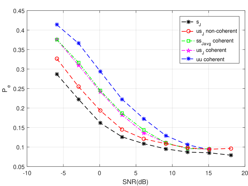
Refer to caption

(i)

Refer to caption

(ii)

Refer to caption

(iii)

Refer to caption

(iv)

Figure 1: Probability of error vs SNR when sensors closer to FC have less probability of error (i) M=2, N=5, (ii) M=2, N=10, iii) M=4, N=5, iv) M=4, N=10.
Refer to caption

(i)

Refer to caption

(ii)

Refer to caption

(iii)

Refer to caption

(iv)

Figure 2: Probability of error vs SNR when sensors farther from FC have less probability of error (i) M=2, N=5, (ii) M=2, N=10, iii) M=4, N=5, iv) M=4, N=10.
Refer to caption

(i)

Refer to caption

(ii)

Refer to caption

(iii)

Refer to caption

(iv)

Figure 3: Probability of error vs SNR when sensors are situated in equal distance from FC with different performance, (i) M=2, N=5, (ii) M=2, N=10 iii) M=4, N=5, iv) M=4, N=10.
Refer to caption

(i)

Refer to caption

(ii)

Refer to caption

(iii)

Refer to caption

(iv)

Figure 4: Probability of error vs SNR when sensors have equal probability of error but in different distance from sensors (i) M=2, N=5 (ii) M=2, N=10 iii) M=4, N=5, iv) M=4, N=10.
Refer to caption

(i)

Refer to caption

(iii)

Figure 5: Probability of error vs rdsubscript𝑟𝑑r_{d} for M=2𝑀2M=2 when sensors closer to FC have less probability of error, (i) N=5 (ii) N=10.
Refer to caption

(i)

Refer to caption

(iii)

Figure 6: Probability of error vs rdsubscript𝑟𝑑r_{d} for M=2𝑀2M=2 and different receptions when sensors farther from FC have less probability of error, (i) N=5 (ii N=10.
Refer to caption

(i)

Refer to caption

(ii)

Figure 7: Probability of error vs rdsubscript𝑟𝑑r_{d} for M=2𝑀2M=2 and different receptions when sensors are situated in equal distance from FC with different performance, (i) N=5, (ii) N=10.
Refer to caption

(i)

Refer to caption

(ii)

Figure 8: Probability of error vs rdsubscript𝑟𝑑r_{d} for M=2𝑀2M=2 when sensors have equal probability of error but in different distance from FC (i) N=5 (ii) N=10.

In this section, numerical results are provided to illustrate the power allocation scheme developed in this paper. In the simulations, we consider the following settings. There are N𝑁N sensors scattered around a FC and the distances from the sensors to the FC are {dk}k=1Nsuperscriptsubscriptsubscript𝑑𝑘𝑘1𝑁\left\{d_{k}\right\}_{k=1}^{N} which we consider to be dk=2+2(k1)subscript𝑑𝑘22𝑘1d_{k}=2+2(k-1) for N=5𝑁5N=5 and dk=ksubscript𝑑𝑘𝑘d_{k}=k for N=10𝑁10N=10. The path loss of signal power at the FC from sensor k follows the Motley-Keenan path loss model (expressed in dB) without the wall and floor attenuation factor [27]: PLk=PL0+10nlog10(dk/d0)𝑃subscript𝐿𝑘𝑃subscript𝐿010𝑛𝑙𝑜𝑔10subscript𝑑𝑘𝑑0PL_{k}=PL_{0}+10nlog10(d_{k}/d0) where PL0𝑃subscript𝐿0PL_{0} is a constant set to 555555dB, and d0subscript𝑑0d_{0} is also a constant set to 1m1𝑚1m in the simulations. Here, n𝑛n is the path loss exponent, which is set to 222 for free space propagation. The variance of channel from sensor k𝑘k to FC is σhk2=PLksubscriptsuperscript𝜎2subscript𝑘𝑃𝐿𝑘\sigma^{2}_{h_{k}}=-PLk. The noise variance from sensors to FC is σn2=30dBmsubscriptsuperscript𝜎2𝑛30𝑑𝐵𝑚\sigma^{2}_{n}=−30dBm dBm. We define the SNR as SNR=10log10Ptot×kσhk2N2σn2𝑆𝑁𝑅10𝑙𝑜subscript𝑔10subscript𝑃𝑡𝑜𝑡subscript𝑘superscriptsubscript𝜎subscript𝑘2superscript𝑁2superscriptsubscript𝜎𝑛2SNR=10log_{10}\frac{P_{tot}\times\sum_{k}\sigma_{h_{k}}^{2}}{N^{2}\sigma_{n}^{2}}. The FC make the final decision rule based on Bayesian criterion rule which depends on the performance of sensors and their quality of channels. The performance of sensors may vary according to their local observation qualities. We will consider three receivers: 1) Coherent reception with channel estimation . 2) Non coherent reception with amplitude estimation. 3) Non coherent reception with channel statistic. In general, We will investigate 4 different cases:
Case V-A1: Sensors closer to FC have less probability of error.
Case V-A2: Sensors farther from FC have less probability of error.
Case V-A3: All Sensors have the same distance from FC.
Case V-A4: All Sensors have the same probability of error but in different distance from FC.
The probability of error for decision of sensor k𝑘k after its observation is: Pes(k)superscriptsubscript𝑃𝑒𝑠𝑘P_{e}^{s}(k): m=1Mim1iMπmpimksuperscriptsubscript𝑚1𝑀subscript𝑖𝑚1𝑖𝑀subscript𝜋𝑚superscriptsubscript𝑝𝑖𝑚𝑘\sum_{m=1}^{M}\sum_{\begin{subarray}{c}i\neq m\\ 1\leq i\leq M\end{subarray}}\pi_{m}p_{im}^{k}. If N=5𝑁5N=5, we consider Pes=[0.5,0.5,0.4,0.3,0.1]superscriptsubscript𝑃𝑒𝑠0.50.50.40.30.1P_{e}^{s}=[0.5,0.5,0.4,0.3,0.1]. If N=10,M=2formulae-sequence𝑁10𝑀2N=10,M=2 Pes=[0.5,0.5,0.48,0.46,0.4,0.35,0.3,0.2,0.15,0.1]superscriptsubscript𝑃𝑒𝑠0.50.50.480.460.40.350.30.20.150.1P_{e}^{s}=[0.5,0.5,0.48,0.46,0.4,0.35,0.3,0.2,0.15,0.1] and For M=4,N=10formulae-sequence𝑀4𝑁10M=4,N=10, Pes=[0.75,0.74,0.7,0.68,0.6,0.55,0.45,0.3,0.2,0.1]superscriptsubscript𝑃𝑒𝑠0.750.740.70.680.60.550.450.30.20.1P_{e}^{s}=[0.75,0.74,0.7,0.68,0.6,0.55,0.45,0.3,0.2,0.1]. Fig. 1 represents probability of error vs SNR when sensors closer to fusion center have less probability of error. As we can see, in coherent reception, we can reduce total power 2dB to have the same probability of error with power allocation based on total J divergence or based on average J divergence. Also, we can see probability of error for two systems: power allocation based on average J divergence and power allocation based on conditional J divergence are approximately the same which means even though we get feedback from FC to sensors to become aware of channel coefficients for power allocation, the performance will not be changed. So, we can do power allocation without feedback. In non coherent reception with channel estimation, with our power allocation, the amount of power will be reduced around 5dB and 7dB for non coherent reception with amplitude estimation and non coherent reception statistic, respectively. As we can see in the figure, in non coherent statistic receiver, for SNR’s greater than 8dB, the probability of error is less for uniform power allocation. Regarding comparing which receiver perform better, The result in this case shows that non coherent statistic perform better for N=5. For N=10, in SNR’s less than 8dB non coherent statistic receiver with power allocation based on total J divergence perform better. In higher SNR’s, coherent receiver and non coherent statistic receiver with uniform power allocation have the best performance. Fig. 2 and Fig. 3 represents probability of error vs SNR for the cases when sensors farther from FC perform better and the case when sensors are situated in equal distance from FC(2m). In these case, we can see similar results to the case when sensors closer to FC perform better. One difference is that in this case the probability of error for coherent reception and power allocation based on average J divergence is worth than power allocation based on conditional J divergence. Fig 4. Represents probability of error vs SNR for the case when sensors have equal performance but they are in different distance from FC. As we can see, our scheme for power allocation, its performance is close to uniform power allocation which indicates the dependency of power allocation to performance of sensors. Fig.5 through Fig.8 represent probability of error vs rtsubscript𝑟𝑡r_{t} for four different cases. The results show that the optimal rtsubscript𝑟𝑡r_{t} for coherent reception is 0.5 and 1 for non coherent reception which means in coherent reception, we should divide power equally between data and training and in non coherent reception, we should devote all power to data.

VI Conclusion

In summary, we considered a distributed detection wireless system that is tasked with solving an M-ary hypothesis testing problem. We studied the effect of wireless channel uncertainty, due to channel estimation error, on the design and performance of this system, assuming the sum of transmit powers of training and data symbols is fixed. In particular, we provided the optimal MAP fusion rules for training and non-training based systems. Then, we have developed a power allocation scheme to distribute the total training and data power budget among the sensors so that the probability of error at the FC is minimized in terms of the conditional J-divergence and average divergence for different receivers. Our analytic results show that average divergence for coherent reception will be maximized when the transmit power is equally distributed between training and data symbols. The simulation results also show that the error probability of this system is minimized when the transmit power is equally distributed between training and data symbols.However, when the sensors employ PSK modulation along with coherent reception at the FC the error probability is minimized when the transmit power is equally distributed between training and data symbols.

Appendix A

The proof of lemma 1 is as below:

PdkJtot|𝑮^subscript𝑃𝑑𝑘subscript𝐽conditional𝑡𝑜𝑡^𝑮\displaystyle\frac{\partial}{\partial P_{dk}}\!\!\!J_{tot|\hat{\boldsymbol{G}}} =i=1Mj=1M𝒈^kσn2(γijkBk(j))(σn2+σh~k2Pdk+𝒈^PdkBi(k))2absentsuperscriptsubscript𝑖1𝑀superscriptsubscript𝑗1𝑀subscript^𝒈𝑘subscriptsuperscript𝜎2𝑛superscriptsubscript𝛾𝑖𝑗𝑘subscript𝐵𝑘𝑗superscriptsubscriptsuperscript𝜎2𝑛subscriptsuperscript𝜎2subscript~𝑘subscript𝑃𝑑𝑘^𝒈subscript𝑃𝑑𝑘subscript𝐵𝑖𝑘2\displaystyle=\sum_{i=1}^{M}\sum_{j=1}^{M}\frac{\hat{\boldsymbol{g}}_{k}\sigma^{2}_{n}\left(\gamma_{ij}^{k}-B_{k}\left(j\right)\right)}{\left(\sigma^{2}_{n}+\sigma^{2}_{\tilde{h}_{k}}P_{dk}+\hat{\boldsymbol{g}}P_{dk}B_{i}\left(k\right)\right)^{2}}
+𝒈^kσn2(γjikBk(i))(σn2+σh~k2Pdk+𝒈^kPdkBj(k))2subscript^𝒈𝑘subscriptsuperscript𝜎2𝑛superscriptsubscript𝛾𝑗𝑖𝑘subscript𝐵𝑘𝑖superscriptsubscriptsuperscript𝜎2𝑛subscriptsuperscript𝜎2subscript~𝑘subscript𝑃𝑑𝑘subscript^𝒈𝑘subscript𝑃𝑑𝑘subscript𝐵𝑗𝑘2\displaystyle+\frac{\hat{\boldsymbol{g}}_{k}\sigma^{2}_{n}\left(\gamma_{ji}^{k}-B_{k}\left(i\right)\right)}{\left(\sigma^{2}_{n}+\sigma^{2}_{\tilde{h}_{k}}P_{dk}+\hat{\boldsymbol{g}}_{k}P_{dk}B_{j}\left(k\right)\right)^{2}}

After some calculation, the term inside the sum will become:

σn2𝒈^k(Bk(j)Bk(i))2(2σn2+2σh~k2Pdk+𝒈^kPdk(Bj(j)+Bk(i)))(σn2+σh~k2Pdk+𝒈^kPdkBj(k))2(σn2+σh~k2Pdk+𝒈^kPdkBi(k))2subscriptsuperscript𝜎2𝑛subscript^𝒈𝑘superscriptsubscript𝐵𝑘𝑗subscript𝐵𝑘𝑖22subscriptsuperscript𝜎2𝑛2subscriptsuperscript𝜎2subscript~𝑘subscript𝑃𝑑𝑘subscript^𝒈𝑘subscript𝑃𝑑𝑘subscript𝐵𝑗𝑗subscript𝐵𝑘𝑖superscriptsubscriptsuperscript𝜎2𝑛subscriptsuperscript𝜎2subscript~𝑘subscript𝑃𝑑𝑘subscript^𝒈𝑘subscript𝑃𝑑𝑘subscript𝐵𝑗𝑘2superscriptsubscriptsuperscript𝜎2𝑛subscriptsuperscript𝜎2subscript~𝑘subscript𝑃𝑑𝑘subscript^𝒈𝑘subscript𝑃𝑑𝑘subscript𝐵𝑖𝑘2\displaystyle\!\!\!\frac{\sigma^{2}_{n}\hat{\boldsymbol{g}}_{k}\left(B_{k}(j)-B_{k}(i)\right)^{2}\left(2\sigma^{2}_{n}+2\sigma^{2}_{\tilde{h}_{k}}P_{dk}+\hat{\boldsymbol{g}}_{k}P_{dk}\left(B_{j}(j)+B_{k}(i)\right)\right)}{\left(\sigma^{2}_{n}+\sigma^{2}_{\tilde{h}_{k}}P_{dk}+\hat{\boldsymbol{g}}_{k}P_{dk}B_{j}\left(k\right)\right)^{2}\left(\sigma^{2}_{n}+\sigma^{2}_{\tilde{h}_{k}}P_{dk}+\hat{\boldsymbol{g}}_{k}P_{dk}B_{i}\left(k\right)\right)^{2}}
+|Bi(k)Bj(k)|2(σn2+σh~k2Pdk+𝒈^kPdkBi(k))2+|Bi(k)Bj(k)|2(σn2+σh~k2Pdk+𝒈^kPdkBj(k))20superscriptsubscript𝐵𝑖𝑘subscript𝐵𝑗𝑘2superscriptsubscriptsuperscript𝜎2𝑛subscriptsuperscript𝜎2subscript~𝑘subscript𝑃𝑑𝑘subscript^𝒈𝑘subscript𝑃𝑑𝑘subscript𝐵𝑖𝑘2superscriptsubscript𝐵𝑖𝑘subscript𝐵𝑗𝑘2superscriptsubscriptsuperscript𝜎2𝑛subscriptsuperscript𝜎2subscript~𝑘subscript𝑃𝑑𝑘subscript^𝒈𝑘subscript𝑃𝑑𝑘subscript𝐵𝑗𝑘20\displaystyle\!\!\!+\frac{|B_{i}(k)-B_{j}(k)|^{2}}{\left(\sigma^{2}_{n}+\sigma^{2}_{\tilde{h}_{k}}P_{dk}+\hat{\boldsymbol{g}}_{k}P_{dk}B_{i}\left(k\right)\right)^{2}}+\frac{|B_{i}(k)-B_{j}(k)|^{2}}{\left(\sigma^{2}_{n}+\sigma^{2}_{\tilde{h}_{k}}P_{dk}+\hat{\boldsymbol{g}}_{k}P_{dk}B_{j}\left(k\right)\right)^{2}}\geq 0

Therefore PdjJtot|𝑮^(Pd1,···,PdN)|Pdk00evaluated-atsubscript𝑃𝑑𝑗subscript𝐽conditional𝑡𝑜𝑡^𝑮subscript𝑃𝑑1···subscript𝑃𝑑𝑁subscript𝑃𝑑𝑘00\frac{\partial}{\partial P_{dj}}J_{tot|\hat{\boldsymbol{G}}}(P_{d1},\textperiodcentered\textperiodcentered\textperiodcentered,P_{dN})|_{P_{dk}\geq 0}\geq 0.
The first order derivative of objective function respect to Ptjsubscript𝑃𝑡𝑗P_{tj} is Jtot|𝑮^Ptj=Jtot|𝑮^𝒈^k𝒈^kPtj+Jtot|𝑮^σwk2σwk2Ptjsubscript𝐽conditional𝑡𝑜𝑡^𝑮subscript𝑃𝑡𝑗subscript𝐽conditional𝑡𝑜𝑡^𝑮subscriptbold-^𝒈𝑘subscriptbold-^𝒈𝑘subscript𝑃𝑡𝑗subscript𝐽conditional𝑡𝑜𝑡^𝑮superscriptsubscript𝜎subscript𝑤𝑘2superscriptsubscript𝜎subscript𝑤𝑘2subscript𝑃𝑡𝑗\frac{\partial J_{tot|\hat{\boldsymbol{G}}}}{\partial P_{tj}}=\frac{\partial J_{tot|\hat{\boldsymbol{G}}}}{\partial\boldsymbol{\hat{g}}_{k}}\frac{\partial\boldsymbol{\hat{g}}_{k}}{\partial P_{tj}}+\frac{\partial J_{tot|\hat{\boldsymbol{G}}}}{\partial\sigma_{w_{k}}^{2}}\frac{\partial\sigma_{w_{k}}^{2}}{\partial P_{tj}}. Similarly, we can prove that Jtot|𝑮^𝒈^k0subscript𝐽conditional𝑡𝑜𝑡^𝑮subscriptbold-^𝒈𝑘0\frac{\partial J_{tot|\hat{\boldsymbol{G}}}}{\partial\boldsymbol{\hat{g}}_{k}}\geq 0 and Jtot|𝑮^σwk20subscript𝐽conditional𝑡𝑜𝑡^𝑮superscriptsubscript𝜎subscript𝑤𝑘20\frac{\partial J_{tot|\hat{\boldsymbol{G}}}}{\partial\sigma_{w_{k}}^{2}}\leq 0. Since 𝒈^kPtj0subscriptbold-^𝒈𝑘subscript𝑃𝑡𝑗0\frac{\partial\boldsymbol{\hat{g}}_{k}}{\partial P_{tj}}\geq 0 and σwk2Ptj0superscriptsubscript𝜎subscript𝑤𝑘2subscript𝑃𝑡𝑗0\frac{\partial\sigma_{w_{k}}^{2}}{\partial P_{tj}}\leq 0, we can conclude Jtot|𝑮^Ptj0subscript𝐽conditional𝑡𝑜𝑡^𝑮subscript𝑃𝑡𝑗0\frac{\partial J_{tot|\hat{\boldsymbol{G}}}}{\partial P_{tj}}\geq 0.

Appendix B

The proof of lemma 2 is as below:
The first order derivative of Javgsubscript𝐽𝑎𝑣𝑔J_{avg} respect to rksubscript𝑟𝑘r_{k} is:

Javgrksubscript𝐽𝑎𝑣𝑔subscript𝑟𝑘\displaystyle\frac{\partial J_{avg}}{\partial r_{k}} =\displaystyle= i=1Mj=1M(1γjikBi(k))xkrkD(xkBi(k))xksuperscriptsubscript𝑖1𝑀superscriptsubscript𝑗1𝑀1superscriptsubscript𝛾𝑗𝑖𝑘subscript𝐵𝑖𝑘subscript𝑥𝑘subscript𝑟𝑘𝐷subscript𝑥𝑘subscript𝐵𝑖𝑘subscript𝑥𝑘\displaystyle\sum_{i=1}^{M}\sum_{j=1}^{M}\left(1-\frac{\gamma_{ji}^{k}}{B_{i}(k)}\right)\frac{\partial x_{k}}{\partial r_{k}}\frac{\partial D\left(\frac{x_{k}}{B_{i}(k)}\right)}{\partial x_{k}}
+(1γijkBj(k))xkrkD(xkBi(k))xk1superscriptsubscript𝛾𝑖𝑗𝑘subscript𝐵𝑗𝑘subscript𝑥𝑘subscript𝑟𝑘𝐷subscript𝑥𝑘subscript𝐵𝑖𝑘subscript𝑥𝑘\displaystyle+\left(1-\frac{\gamma_{ij}^{k}}{B_{j}(k)}\right)\frac{\partial x_{k}}{\partial r_{k}}\frac{\partial D\left(\frac{x_{k}}{B_{i}(k)}\right)}{\partial x_{k}}

Now, We prove that D(x)𝐷𝑥D(x) is an increasing function of x𝑥x. We show that D(x2)D(x1)𝐷subscript𝑥2𝐷subscript𝑥1D(x_{2})\geq D(x_{1}) if x2x1subscript𝑥2subscript𝑥1x_{2}\geq x_{1}.

D(x2)D(x1)𝐷subscript𝑥2𝐷subscript𝑥1\displaystyle D(x_{2})-D(x_{1}) =\displaystyle= x2ex2x2ett𝑑tx1ex1x1ett𝑑tsubscript𝑥2superscript𝑒subscript𝑥2superscriptsubscriptsubscript𝑥2superscript𝑒𝑡𝑡differential-d𝑡subscript𝑥1superscript𝑒subscript𝑥1superscriptsubscriptsubscript𝑥1superscript𝑒𝑡𝑡differential-d𝑡\displaystyle x_{2}e^{x_{2}}\int_{x_{2}}^{\infty}\frac{e^{-t}}{t}dt-x_{1}e^{x_{1}}\int_{x_{1}}^{\infty}\frac{e^{-t}}{t}dt
0et(x2t+x2x1t+x2)𝑑tsuperscriptsubscript0superscript𝑒𝑡subscript𝑥2𝑡subscript𝑥2subscript𝑥1𝑡subscript𝑥2differential-d𝑡\displaystyle\int_{0}^{\infty}e^{-t}\left(\frac{x_{2}}{t+x_{2}}-\frac{x_{1}}{t+x_{2}}\right)dt
0et(tx2tx1(t+x2)(t+x1))𝑑t0superscriptsubscript0superscript𝑒𝑡𝑡subscript𝑥2𝑡subscript𝑥1𝑡subscript𝑥2𝑡subscript𝑥1differential-d𝑡0\displaystyle\int_{0}^{\infty}e^{-t}\left(\frac{tx_{2}-tx_{1}}{\left(t+x_{2}\right)\left(t+x_{1}\right)}\right)dt\geq 0

Therefore, D(x)x0𝐷𝑥𝑥0\frac{\partial D(x)}{\partial x}\geq 0.
Based on the assumption of (1γjikBi(k))<01superscriptsubscript𝛾𝑗𝑖𝑘subscript𝐵𝑖𝑘0\left(1-\frac{\gamma_{ji}^{k}}{B_{i}(k)}\right)<0 and xkrksubscript𝑥𝑘subscript𝑟𝑘\frac{\partial x_{k}}{\partial r_{k}}, we will have:

{Javgrk>0,ifrk<12Javgrk=0,ifrk=12Javgrk<0,ifrk>12casessubscript𝐽𝑎𝑣𝑔subscript𝑟𝑘0ifsubscript𝑟𝑘12subscript𝐽𝑎𝑣𝑔subscript𝑟𝑘0ifsubscript𝑟𝑘12subscript𝐽𝑎𝑣𝑔subscript𝑟𝑘0ifsubscript𝑟𝑘12\begin{cases}\frac{\partial J_{avg}}{\partial r_{k}}>0,&\text{if}\ r_{k}<\frac{1}{2}\\ \frac{\partial J_{avg}}{\partial r_{k}}=0,&\text{if}\ r_{k}=\frac{1}{2}\\ \frac{\partial J_{avg}}{\partial r_{k}}<0,&\text{if}\ r_{k}>\frac{1}{2}\end{cases}

Based on above relationship, when rk<12subscript𝑟𝑘12r_{k}<\frac{1}{2}, Javgsubscript𝐽𝑎𝑣𝑔J_{avg} is an increasing function of rksubscript𝑟𝑘r_{k} and for rk>12subscript𝑟𝑘12r_{k}>\frac{1}{2}, Javgsubscript𝐽𝑎𝑣𝑔J_{avg} is a decreasing function of rksubscript𝑟𝑘r_{k}. Therefore, we can conclude the optimal rk=0.5superscriptsubscript𝑟𝑘0.5r_{k}^{*}=0.5.

Appendix C

The proof of lemma 3 is as below:
The first derivative of Javgsubscript𝐽𝑎𝑣𝑔J_{avg} respect to Pksubscript𝑃𝑘P_{k} is

i=1Mj=1MfkxkxkPk=i=1Mj=1M(fk1xk+fk2xk)xkPksuperscriptsubscript𝑖1𝑀superscriptsubscript𝑗1𝑀subscript𝑓𝑘subscript𝑥𝑘subscript𝑥𝑘subscript𝑃𝑘superscriptsubscript𝑖1𝑀superscriptsubscript𝑗1𝑀superscriptsubscript𝑓𝑘1subscript𝑥𝑘superscriptsubscript𝑓𝑘2subscript𝑥𝑘subscript𝑥𝑘subscript𝑃𝑘\sum_{i=1}^{M}\sum_{j=1}^{M}\frac{\partial f_{k}}{\partial x_{k}}\frac{\partial x_{k}}{\partial P_{k}}=\sum_{i=1}^{M}\sum_{j=1}^{M}\left(\frac{\partial f_{k}^{1}}{\partial x_{k}}+\frac{\partial f_{k}^{2}}{\partial x_{k}}\right)\frac{\partial x_{k}}{\partial P_{k}} (38)

Where fksubscript𝑓𝑘f_{k} is:

fk=i=1Mj=1M[γjikBi(k)+(1γjikBi(k))D(xkBi(k))]subscript𝑓𝑘superscriptsubscript𝑖1𝑀superscriptsubscript𝑗1𝑀delimited-[]superscriptsubscript𝛾𝑗𝑖𝑘subscript𝐵𝑖𝑘1superscriptsubscript𝛾𝑗𝑖𝑘subscript𝐵𝑖𝑘𝐷subscript𝑥𝑘subscript𝐵𝑖𝑘\displaystyle\!\!\!\!\!\!\!\!\!\!\!f_{k}=\sum_{i=1}^{M}\sum_{j=1}^{M}\left[\frac{\gamma_{ji}^{k}}{B_{i}(k)}+\left(1-\frac{\gamma_{ji}^{k}}{B_{i}(k)}\right)D(\frac{x_{k}}{B_{i}(k)})\right]
[i=1Mj=1M+γijkBj(k)+(1γijkBj(k))D(xkBj(k))]delimited-[]superscriptsubscript𝑖1𝑀superscriptsubscript𝑗1𝑀superscriptsubscript𝛾𝑖𝑗𝑘subscript𝐵𝑗𝑘1superscriptsubscript𝛾𝑖𝑗𝑘subscript𝐵𝑗𝑘𝐷subscript𝑥𝑘subscript𝐵𝑗𝑘\displaystyle\left[\sum_{i=1}^{M}\sum_{j=1}^{M}+\frac{\gamma_{ij}^{k}}{B_{j}(k)}+\left(1-\frac{\gamma_{ij}^{k}}{B_{j}(k)}\right)D(\frac{x_{k}}{B_{j}(k)})\right]

The derivative of first bracket respect to Pksubscript𝑃𝑘P_{k} become:

i=1Mj=1M(1γjikBi(k))DxkxkPksuperscriptsubscript𝑖1𝑀superscriptsubscript𝑗1𝑀1superscriptsubscript𝛾𝑗𝑖𝑘subscript𝐵𝑖𝑘𝐷subscript𝑥𝑘subscript𝑥𝑘subscript𝑃𝑘\sum_{i=1}^{M}\sum_{j=1}^{M}\left(1-\frac{\gamma_{ji}^{k}}{B_{i}(k)}\right)\frac{\partial D}{\partial x_{k}}\frac{\partial x_{k}}{\partial P_{k}} (39)

Since D(x)/(x)0𝐷𝑥𝑥0\partial D(x)/\partial(x)\geq 0, 1γjikBi(k)<01superscriptsubscript𝛾𝑗𝑖𝑘subscript𝐵𝑖𝑘01-\frac{\gamma_{ji}^{k}}{B_{i}(k)}<0, xk/Pk0subscript𝑥𝑘subscript𝑃𝑘0\partial x_{k}/\partial P_{k}\leq 0, we conclude that The derivative of first bracket is non negative. Similarly, We can see that derivative of second bracket in (C) is non negative. Therefore, We conclude that Javg/Pk0subscript𝐽𝑎𝑣𝑔subscript𝑃𝑘0\partial J_{avg}/\partial P_{k}\geq 0.

References

  • [1] Ruixin Niu, Biao Chen, and P.K. Varshney. Fusion of decisions transmitted over rayleigh fading channels in wireless sensor networks. Signal Processing, IEEE Transactions on, 54(3):1018–1027, March 2006.
  • [2] F. Jiang, J. Chen, A. L. Swindlehurst, and J. A. López-Salcedo. Massive mimo for wireless sensing with a coherent multiple access channel. IEEE Transactions on Signal Processing, 63(12):3005–3017, June 2015.
  • [3] H. He and P. K. Varshney. Fusing censored dependent data for distributed detection. IEEE Transactions on Signal Processing, 63(16):4385–4395, Aug 2015.
  • [4] P. Braca, S. Marano, and V. Matta. Single-transmission distributed detection via order statistics. IEEE Transactions on Signal Processing, 60(4):2042–2048, April 2012.
  • [5] V. S. S. Nadendla and P. K. Varshney. Design of binary quantizers for distributed detection under secrecy constraints. IEEE Transactions on Signal Processing, 64(10):2636–2648, May 2016.
  • [6] Xin Zhang, H.V. Poor, and Mung Chiang. Optimal power allocation for distributed detection over mimo channels in wireless sensor networks. Signal Processing, IEEE Transactions on, 56(9):4124–4140, Sept 2008.
  • [7] M.K. Banavar, A.D. Smith, C. Tepedelenlioglu, and A. Spanias. On the effectiveness of multiple antennas in distributed detection over fading macs. Wireless Communications, IEEE Transactions on, 11(5):1744–1752, May 2012.
  • [8] A. Vosoughi and Yupeng Jia. How does channel estimation error affect average sum-rate in two-way amplify-and-forward relay networks? Wireless Communications, IEEE Transactions on, 11(5):1676–1687, May 2012.
  • [9] H.R. Ahmadi and A. Vosoughi. Impact of wireless channel uncertainty upon distributed detection systems. Wireless Communications, IEEE Transactions on, 12(6):2566–2577, June 2013.
  • [10] H.R. Ahmadi and A. Vosoughi. Impact of channel estimation error on decentralized detection in bandwidth constrained wireless sensor networks. In Military Communications Conference, 2008. MILCOM 2008. IEEE, pages 1–7, Nov 2008.
  • [11] I. Nevat, G.W. Peters, and I.B. Collings. Distributed detection in sensor networks over fading channels with multiple antennas at the fusion center. Signal Processing, IEEE Transactions on, 62(3):671–683, Feb 2014.
  • [12] C. R. Berger, M. Guerriero, S. Zhou, and P. Willett. Pac vs. mac for decentralized detection using noncoherent modulation. IEEE Transactions on Signal Processing, 57(9):3562–3575, Sept 2009.
  • [13] F. Li, J. S. Evans, and S. Dey. Decision fusion over noncoherent fading multiaccess channels. IEEE Transactions on Signal Processing, 59(9):4367–4380, Sept 2011.
  • [14] D. Ciuonzo, G. Romano, and P. Salvo Rossi. Optimality of received energy in decision fusion over rayleigh fading diversity mac with non-identical sensors. IEEE Transactions on Signal Processing, 61(1):22–27, Jan 2013.
  • [15] N. Maleki, A. Vosoughi, and N. Rahnavard. Distributed binary detection over fading channels: Cooperative and parallel architectures. IEEE Transactions on Vehicular Technology, 65(9):7090–7109, Sept 2016.
  • [16] Jayesh H. Kotecha, V. Ramachandran, and A.M. Sayeed. Distributed multitarget classification in wireless sensor networks. Selected Areas in Communications, IEEE Journal on, 23(4):703–713, April 2005.
  • [17] N. Maleki and A. Vosoughi. Channel-aware m-ary distributed detection: Optimal and suboptimal fusion rules. In Statistical Signal Processing Workshop (SSP), 2012 IEEE, pages 644–647, Aug 2012.
  • [18] A. Jeremic, Kon Max Wong, and Bin Liu. Optimal distributed detection of multiple hypotheses using blind algorithm. In Acoustics, Speech and Signal Processing, 2009. ICASSP 2009. IEEE International Conference on, pages 2241–2244, April 2009.
  • [19] E. Nurellari, D. McLernon, and M. Ghogho. Distributed two-step quantized fusion rules via consensus algorithm for distributed detection in wireless sensor networks. IEEE Transactions on Signal and Information Processing over Networks, 2(3):321–335, Sept 2016.
  • [20] J. A. Maya, L. Rey Vega, and C. G. Galarza. Optimal resource allocation for detection of a gaussian process using a mac in wsns. IEEE Transactions on Signal Processing, 63(8):2057–2069, April 2015.
  • [21] M. Najimi, A. Ebrahimzadeh, S. M. H. Andargoli, and A. Fallahi. Energy-efficient sensor selection for cooperative spectrum sensing in the lack or partial information. IEEE Sensors Journal, 15(7):3807–3818, July 2015.
  • [22] Z. Xu, J. Huang, and Q. Zhang. Power constrained partially coherent distributed detection over fading multiaccess channels. IEEE Sensors Journal, 13(7):2729–2736, July 2013.
  • [23] Hyoung-Soo Kim and N.A. Goodman. Power control strategy for distributed multiple-hypothesis detection. Signal Processing, IEEE Transactions on, 58(7):3751–3764, July 2010.
  • [24] Mokhtar S. Bazaraa. Nonlinear Programming: Theory and Algorithms. Wiley Publishing, 3rd edition, 2013.
  • [25] H. Senol and C. Tepedelenlioglu. Performance of distributed estimation over unknown parallel fading channels. IEEE Transactions on Signal Processing, 56(12):6057–6068, Dec 2008.
  • [26] Muhammad Hafeez Chaudhary and Luc Vandendorpe. Adaptive power allocation in wireless sensor networks with spatially correlated data and analog modulation: Perfect and imperfect csi. EURASIP J. Wirel. Commun. Netw., 2010:12:1–12:14, January 2010.
  • [27] A. J. Motley and J. M. P. Keenan. Personal communication radio coverage in buildings at 900 MHz and 1700 MHz. Electronics Letters., vol. 24, no. 12, pp. 763-764, 9 June 1988.