Finite-temperature phase transition to a Kitaev spin liquid phase
on a hyperoctagon lattice: A large-scale quantum Monte Carlo study

Abstract

The quantum spin liquid is an enigmatic quantum state in insulating magnets, in which conventional long-range order is suppressed by strong quantum fluctuations. Recently, an unconventional phase transition was reported between the low-temperature quantum spin liquid and the high-temperature paramagnet in the Kitaev model on a three-dimensional hyperhoneycomb lattice. Here, we show that a similar “liquid-gas” transition takes place in another three-dimensional lattice, the hyperoctagon lattice. We investigate the critical phenomena by adopting the Green-function based Monte Carlo technique with the kernel polynomial method, which enables systematic analysis of up to $2048$ sites. The critical temperature is lower than that in the hyperhoneycomb case, reflecting the smaller flux gap. We also discuss the transition on the basis of an effective model in the anisotropic limit.

I Introduction

The quantum spin liquid (QSL) is an exotic magnetic state of matter in solids, in which long-range ordering is suppressed by strong quantum fluctuations even in the ground state Anderson (1973); Fazekas and Anderson (1974); Balents (2010). As a consequence of intensive study over several decades, substantial progress has been recently made in experimental search for QSLs Kanoda and Kato (2011); Gingras and McClarty (2014); Okamoto et al. (2007); Coldea et al. (2003); Hiroi et al. (2001); Shores et al. (2005); Okamoto et al. (2009); Han et al. (2014). In such experiments, however, QSLs are usually identified by the absence of any phase transition to a long-range ordered state. In other words, it is supposed that the low-temperature ($T$) QSL is adiabatically connected to the high-$T$ paramagnetic state. This common belief relies on the magnetic analog of liquid helium $3$ which remains as a liquid down to the lowest $T$ due to strong quantum fluctuations Anderson (1973). Nonetheless, in conventional fluids, gas and liquid can be distinguished by a phase transition. Hence, a similar phase transition can also be expected in the case of magnetic states of matter, namely, between the “spin gas” (paramagnet) and “spin liquid” (QSL). However, the thermodynamics of QSLs remains elusive, despite the crucial importance for understanding of existing and forthcoming experiments.

Recently, an exotic finite-$T$ phase transition between the low-$T$ QSL and the high-$T$ paramagnet was reported for an extension of the Kitaev model defined on a three-dimensional (3D) hyperhoneycomb lattice as well as its anisotropic limit Nasu et al. (2014a, b). The Kitaev model is an exactly-soluble quantum spin model, whose ground state provides a canonical example of QSLs Kitaev (2006), and has attracted attention as it might describe the magnetism in some spin-orbit entangled Mott insulatorsJackeli and Khaliullin (2009). The finding of the exotic phase transition was brought by a newly-developed quantum Monte Carlo (QMC) method based on a Majorana fermion representation, which is free from the negative sign problem. This phase transition is not accompanied by any symmetry breaking, but can be explained by a proliferation of loops for excited $Z_{2}$ fluxes Kimchi et al. (2014); Nasu et al. (2014b, a). The emergent loop degree of freedom is specific to 3D; the finite-$T$ phase transition is absent and turns into a crossover in two dimensions Nasu et al. (2015). The surprising result urges reconsideration of both experimental and theoretical quests for QSLs.

As demonstrated in the hyperhoneycomb case Mandal and Surendran (2009), the Kitaev model can be extended to any tri-coordinate lattices Yang et al. (2007); O’Brien et al. (2016); Hermanns and Trebst (2014); Yao and Kivelson (2007). Although all the extensions retain the QSL nature Baskaran et al. (2007), the exact ground state (the spatial configuration of $Z_{2}$ fluxes) is obtained for some limited cases because Lieb’s theorem is not applicable to generic tri-coordinate lattices Lieb (1994). Moreover, finite-$T$ properties have not been studied in most cases. As there are a variety of 3D tri-coordinate lattices O’Brien et al. (2016); Wells (1977), it is interesting to investigate such 3D models for clarifying the universal aspects of the phase transition between the QSL and the paramagnet and for exploring further exotic phase transitions.

In this paper, we investigate finite-$T$ properties in the Kitaev model on another 3D lattice, the hyperoctagon lattice Hermanns and Trebst (2014) (see Fig. 1). For this model, the exact solution is not available, as Lieb’s theorem cannot be applied. Improving the QMC method by employing the Green function technique with the kernel polynomial method (KPM), we compute much larger systems compared to the previous studies. From the systematic analysis of clusters up to $2048$ sites, we find that the hyperoctagon model exhibits another example of finite-$T$ phase transitions between the QSL and the paramagnet. We find that the critical temperature estimated from the careful analysis of the finite-size effects is lower than that for the hyperhoneycomb case, reflecting the smaller flux gap O’Brien et al. (2016); Kimchi et al. (2014). In addition, we show that the anisotropic limit of the hyperoctagon model becomes equivalent to that of the hyperhoneycomb one, which supports the common origin of the phase transition on two lattices.

The paper is structured as follows. In Sec. II, we introduce the Kitaev model on a hyperoctagon lattice, and briefly describe the numerical method used in the previous studies to analyze the finite-$T$ properties of the Kitaev model. Then we introduce the improved QMC method by using the Green-function based KPM (GFb-KPM) and present the benchmark results. In Sec. III, we present numerical results. We identify the finite-$T$ phase transition and estimate the critical temperature from careful analyses of finite-size effects for three different physical quantities. In Sec. IV, we discuss the origin of the phase transition on the hyperoctagon lattice, with a consideration of the anisotropic limit of the model in comparison with that for the hyperhoneycomb case. We also discuss a correlation between the critical temperature and the flux gap, with a brief comment on the ground state. Finally, Sec. V is devoted to the summary.

II Model and Method

We study an extension of the Kitaev model Kitaev (2006) to a 3D hyperoctagon lattice shown in Fig. 1 Hermanns and Trebst (2014). The Hamiltonian is given by

$$\mathcal{H}=-J_{x}\sum_{\langle i,j\rangle_{x}}\sigma_{i}^{x}\sigma_{j}^{x}-J_{y}\sum_{\langle i,j\rangle_{y}}\sigma_{i}^{y}\sigma_{j}^{y}-J_{z}\sum_{\langle i,j\rangle_{z}}\sigma_{i}^{z}\sigma_{j}^{z},$$ (1)

where $\sigma_{i}^{x}$, $\sigma_{i}^{y}$, and $\sigma_{i}^{z}$ are the Pauli matrices describing a spin-$1/2$ state at site $i$. The sum $\langle i,j\rangle_{\gamma}$ is taken over the nearest-neighbor (NN) sites on the three different types of bonds, which are shown by red ($\gamma=x$), green ($y$), and blue ($z$) in Fig. 1; $J_{\gamma}$ is the exchange constant for each bond. Similar to the original Kitaev model on a honeycomb lattice Kitaev (2006), the hyperoctagon model has a $Z_{2}$ conserved quantity called the fluxes for each ten-site plaquette $p$ (see Fig. 1), $W_{p}=\prod_{\langle i,j\rangle_{\gamma}\in p}\sigma_{i}^{\gamma}\sigma_{j}^{\gamma}=\pm 1$, where the product is taken for all the bonds comprising the plaquette. While the ground state of this model is not exactly obtained, it was deduced to be a flux-free state, where all $W_{p}$ are $+1$ Hermanns and Trebst (2014), similar to the honeycomb Kitaev (2006) and hyperhoneycomb cases Mandal and Surendran (2009).

We investigate thermodynamic properties of the model in Eq. (1) by the QMC simulation based on a Majorana fermion representation Nasu et al. (2014a). In this technique, the lattice is regarded as an assembly of one-dimensional chains composed of two types of bonds and the Jordan-Wigner transformation is applied to each chain Chen and Hu (2007); Feng et al. (2007); Chen and Nussinov (2008). By taking such chains along the ${\bf{a}}_{1}$ direction composed of the red and green bonds as in Fig. 1, the Kitaev Hamiltonian in Eq. (1) is rewritten by two types of Majorana fermions $c$ and $\bar{c}$ as

$$\mathcal{H}=iJ_{x}\sum_{(w,b)_{x}}c_{w}c_{b}+iJ_{y}\sum_{(w,b)_{y}}c_{w}c_{b}+iJ_{z}\sum_{(w,b)_{z}}\eta_{r}c_{w}c_{b},$$ (2)

where $\eta_{r}=i\bar{c}_{b}\bar{c}_{w}$ is a local conserved quantity taking $\pm 1$ ($r$ is the index for the $z$ bond); it satisfies $W_{p}=\prod_{r\in p}\eta_{r}$, where the product is taken for all the $z$ bonds included in the ten-site loop. The sum of $(w,b)_{\gamma}$ is taken for the NN sites on the $\gamma$ bonds with $w>b$ ($b>w$) if the chain begins with $b$ ($w$) (see Fig. 1). From the form of Eq. (2), the system is regarded as free Majorana fermions coupled with the $Z_{2}$ variables $\eta_{r}$. Hence, one can compute thermodynamic properties by Monte Carlo (MC) sampling over the configurations $\{\eta_{r}\}$ with the statistical weight $P(\{\eta_{r}\})=\exp[-\beta F(\{\eta_{r}\})]$, where $F(\{\eta_{r}\})$ is the free energy of the Majorana fermions $\{c\}$ for a configuration $\{\eta_{r}\}$, and $\beta=1/T$ is the inverse temperature (we set the Boltzmann constant $k_{\rm B}=1$). As $P(\{\eta_{r}\})$ is positive definite, the QMC simulation is free from the negative sign problem Nasu et al. (2014a); Nasu and Motome (2015); Nasu et al. (2015, 2016).

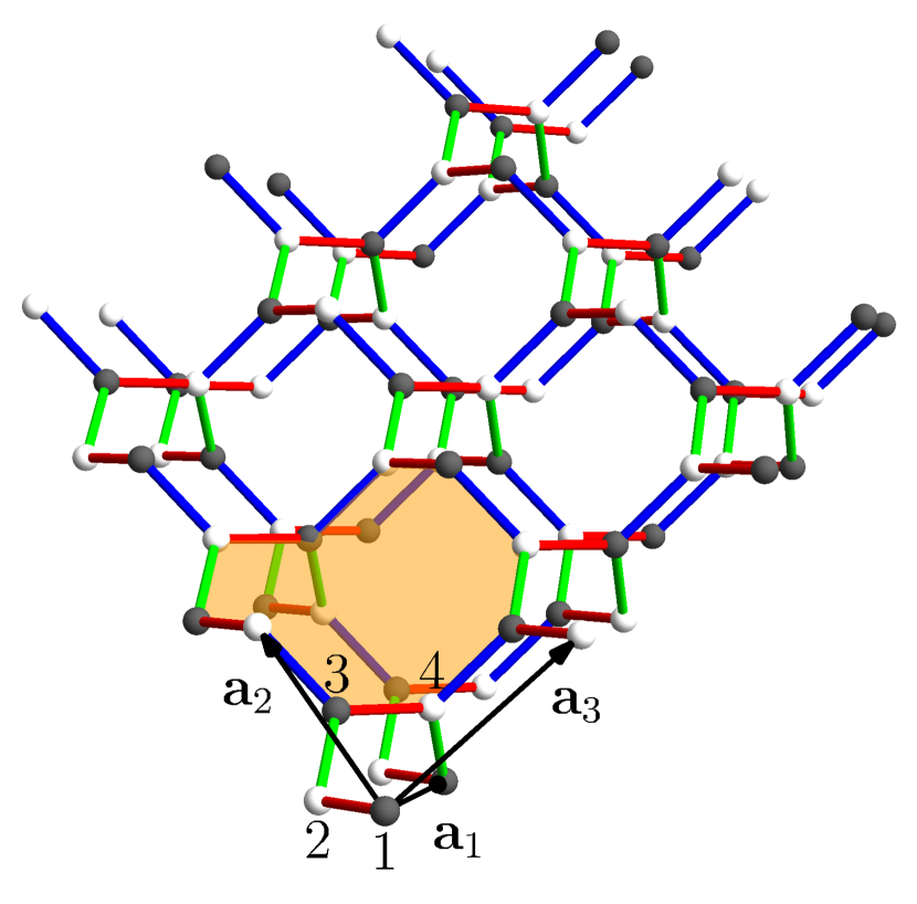
Figure 1: Schematic picture of the hyperoctagon lattice. The spheres represent the lattice sites on which the spin-$1/2$ degrees of freedom are defined in Eq. (1). The sites $1$-$4$ represent the four-site unit cell, and ${\bf{a}}_{\mu}$ ($\mu=1,2,3$) represent the lattice translation vectors. The red, green, and blue bonds denote the $x$, $y$, and $z$ bonds in Eq. (1), respectively. The hyperoctagon lattice is bipartite, and the black $b$ and white $w$ spheres identify the sublattices; see Eq. (2). The orange shade denotes an example of a ten-site plaquette on which the $Z_{2}$ flux $W_{p}$ is defined.

In the previous studies Nasu et al. (2014a); Nasu and Motome (2015); Nasu et al. (2015, 2016), $F(\{\eta_{r}\})$ was calculated by the exact diagonalization (ED), which leads to the computational cost of $\mathcal{O}(N^{4})$ for one MC sweep where $N$ is the number of spins. This has limited the reachable system size $N$ to less than $10^{3}$ in a reasonable computational time. In order to reduce the computational cost and enable systematic analysis of up to larger $N$, in the present study, we apply the GFb-KPM to estimate $F(\{\eta_{r}\})$ Weiße (2009). In this method, a change of the Majorana fermion density of states in a MC update is directly computed from a small number of Green functions obtained by the KPM Weiße et al. (2006), which reduces the computational cost to $\mathcal{O}(N^{2})$.

Let us describe the method briefly. Suppose if the one-body Majorana Hamiltonian for a given configuration $\{\eta_{r}\}$, $\mathcal{H}(\{\eta_{r}\})$, is modified to $\mathcal{H}(\{\eta_{r}\})+\Delta$ by a local flip of $\eta_{r}$, then the energy spectrum is given by the solution of $\mathcal{D}(E)=\mathrm{det}\{\mathbb{I}+G(E)\Delta\}=0$, where $G(E)$ is the Green function satisfying $G(E)\{\mathcal{H}(\{\eta_{r}\})-E\mathbb{I}\}=\mathbb{I}$ ($\mathbb{I}$ is the unit matrix). By extending $\mathcal{D}(E)$ to a complex function by $E\rightarrow E+i\epsilon$, the difference in the free energy by the local flip is given by

$$F(\{\eta_{r}^{\prime}\})-F(\{\eta_{r}\})$$

$$=-\frac{N}{\pi}\int_{0}^{\infty}\lim_{\epsilon\to 0}\operatorname{Im}\ln\{\mathcal{D}(E+i\epsilon)\}\frac{1}{2}\tanh\left(\frac{\beta E}{2}\right)dE.$$ (3)

$\mathcal{D}(E+i\epsilon)$ can be calculated in a compact manner by using a few components of Green’s functions Weiße et al. (2006). The Green functions are obtained by using the KPM with Chebyshev polynomials. For instance, the onsite component is obtained as

$$G_{j,j}(E+i\epsilon)=i\frac{{\mu_{0}}+2\sum_{m=1}^{M-1}{\mu_{m}}\mathrm{exp}\{-im~{}\mathrm{arccos}(E/s)\}}{\sqrt{s^{2}-E^{2}}},$$ (4)

where $\mu_{m}$ is the $j$th diagonal element of the $m$th Chebyshev moment of $\mathcal{H}(\{\eta_{r}\})$ rescaled by a factor of $s$ to fit the eigenvalues in the range of $[-1:1]$, and $M$ is the cutoff of the expansion Weiße (2009). $\mu_{m}$ is calculated efficiently by sparse matrix-vector multiplications Weiße et al. (2006).

In the following calculations, we focus on the isotropic case and set the energy unit as $J_{x}=J_{y}=J_{z}=1/3$. We consider the clusters from $32$ ($2^{3}$ unit cells) to $2048$ sites ($8^{3}$ unit cells) with the open boundary condition in the ${\bf{a}}_{1}$ direction and the periodic ones in the remaining two directions. We typically perform ten independent MC runs with $500$ MC steps for measurements after $3500$ to $5500$ steps for thermalization. In addition to MC sweeps by a single flip of $\eta_{r}$, we adopt the replica exchange MC technique Hukushima and Nemoto (1996).

Figure 2 shows the benchmark of the GFb-KPM method. We compare the QMC data of the specific heat per site, $C_{v}$, computed by the ED method and the GFb-KPM method for the $4\times 4^{3}=256$-site cluster. For the GFb-KPM calculations, we present the data with a different cutoff of the Chebyshev expansion, $M$, from $M=64$ to $512$. Figure 2(a) shows $T$ dependence of $C_{v}$. We find that the GFb-KPM data well converge to the ED ones, even for the smallest $M=64$, except for the low-$T$ region around the low-$T$ peak of $C_{v}$. Figure 2(b) shows the convergence of the GFb-KPM data in terms of $M$ in the low-$T$ region: the symbols indicate the GFb-KPM data for each $M$, while the horizontal lines the ED ones (the dashed lines indicate the statistical errorbars). We find that the GFb-KPM results quickly converge to the ED ones while increasing $M$. On the basis of this benchmark as well as the fact that the GFb-KPM converges faster for larger system sizes Weiße et al. (2006), we take $M=512$ for the $576$-site cluster and $M=256$ for larger clusters in the following GFb-KPM calculations .

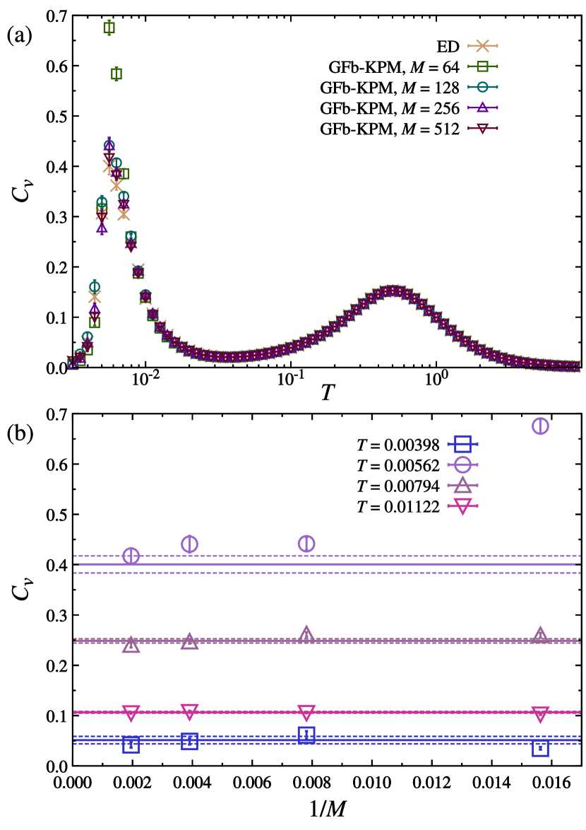
Figure 2: (a) Comparison of the QMC results for the $T$ dependence of the specific heat per site, $C_{v}$, obtained by the update scheme with the ED and GFb-KPM. In the GFb-KPM calculations, the Green functions are obtained by the Chebyshev expansion up to $M=512$. (b) $M$ dependence of $C_{v}$ at several temperatures in the low-$T$ region around the low-$T$ peak in (a). The horizontal solid lines represent the ED results with errorbars indicated by the dashed lines. The calculations are done for the isotropic case $J_{x}=J_{y}=J_{z}=1/3$ in Eq. (1) on the $4\times 4^{3}=256$-site cluster.

III Results

Figure 3(a) shows the QMC results of the specific heat per site, $C_{v}$. Similar to the hyperhoneycomb case Nasu et al. (2014a), $C_{v}$ exhibits two peaks. The higher-$T$ peak is closely related with the development of NN spin correlations $S^{zz}=2\sum_{\langle i,j\rangle_{z}}\langle\sigma_{i}^{z}\sigma_{j}^{z}\rangle/N$ shown in Fig. 3(c), which corresponds to the lowering of the kinetic energy of the itinerant Majorana fermions Nasu et al. (2015, 2014a). On the other hand, the lower-$T$ peak in $C_{v}$ is associated with the coherent alignment of the $Z_{2}$ variables $W_{p}$ Nasu et al. (2015, 2014a); see the thermal average $\bar{W}_{p}=\langle\sum_{p}W_{p}\rangle/N_{p}$ plotted in Fig. 3(c) ($N_{p}$ is the number of ten-site plaquettes in the system). Figure 3(b) shows the results of the entropy per site, $S=\ln 2+\beta\langle\mathcal{H}\rangle/N-\int_{0}^{\beta}\langle\mathcal{H}\rangle d\beta/N$. At each peak of $C_{v}$, a half of $\ln 2$ entropy is released; the higher-$T$ release comes from itinerant Majorana fermions and the lower one comes from $Z_{2}$ variables $W_{p}$. Similar behavior was reported for the Kitaev models on the honeycomb and hyperhoneycomb lattices Nasu et al. (2015, 2014a). This is the common feature in the Kitaev QSLs called thermal fractionalization of quantum spins Nasu et al. (2015).

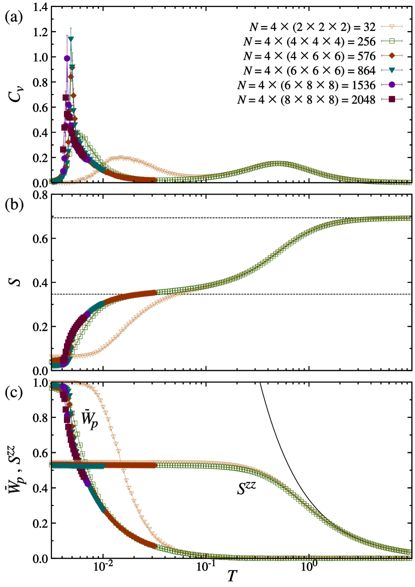
Figure 3: Temperature dependence of (a) $C_{v}$, (b) the entropy per site $S$, and (c) the average of the $Z_{2}$ variables $W_{p}$, $\bar{W}_{p}$, and the NN spin correlation on the $z$ bonds, $S^{zz}$. The calculations were performed for the isotropic case in Eq. (1) on several clusters whose sizes are indicated in the figure. The dashed horizontal lines in (b) indicate $(1/2)\ln 2$ and $\ln 2$. The black curve in (c) represents the high-$T$ asymptotic Curie behavior $1/(3T)$.

In Fig. 3(a), while the high-$T$ peak of $C_{v}$ is almost system-size independent, the low-$T$ peak exhibits significant system-size dependence: the peak becomes sharper and shifts to lower $T$ while increasing the system size. The enlarged view of the low-$T$ part is shown in Fig. 4(a). The system-size dependence is indicative of a phase transition, as in the hyperhoneycomb case Nasu et al. (2014a). We note that the height of the peaks does not show systematic behavior, which is presumably due to the different shapes of clusters. We find similar critical behavior in thermal fluctuations of $W_{p}$, defined by

$$\Delta W_{p}=\frac{(\sum_{\gamma}J_{\gamma})^{2}}{N_{p}T^{2}}\Big{[}\big{\langle}\big{(}\sum_{p}W_{p}\big{)}^{2}\big{\rangle}-\big{\langle}\sum_{p}W_{p}\big{\rangle}^{2}\Big{]}.$$ (5)

As shown in Fig. 4(b), $\Delta W_{p}$ shows a similar peak to $C_{v}$. We note that this quantity gives a measure of the specific heat in the case of the anisotropic limit of the Kitaev model where the Hamiltonian is described by $W_{p}$ only; namely, $\Delta W_{p}$ gives a measure of energy fluctuations related to $W_{p}$. Thus, the common critical behavior between $C_{v}$ and $\Delta W_{p}$ indicates that the phase transition is driven by the $Z_{2}$ variables $W_{p}$.

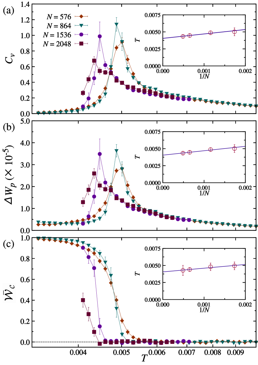
Figure 4: Enlarged views of the low-$T$ region: (a) $C_{v}$, (b) fluctuations of $W_{p}$, $\Delta W_{p}$, and (c) the Wilson loop $\bar{\mathcal{W}}_{c}$. The insets show the system-size extrapolation of the peak $T$ of (a) $C_{v}$ and (b) $\Delta W_{p}$, and (c) the inflection point of $T$ dependence of $\bar{\mathcal{W}}_{c}$.

In order to characterize the phase transition, following the previous study for the hyperhoneycomb case Nasu et al. (2014a), we also measure the Wilson loop $\bar{\mathcal{W}}_{c}$ on a plane perpendicular to one of the periodic boundaries. As shown in Fig. 4(c), $\bar{\mathcal{W}}_{c}$ is zero at high $T$ and grows rapidly in well accordance with the peaks of $C_{v}$ and $\Delta W_{p}$. This behavior is in contrast to the gradual growth of $\bar{W}_{p}$ in Fig. 3(c). The result indicates that the global quantity $\bar{\mathcal{W}}_{c}$ acts as an order parameter for the unconventional phase transition, as in the hyperhoneycomb case Nasu et al. (2014a).

From the critical behaviors of $C_{v}$, $\Delta W_{p}$, and $\bar{\mathcal{W}}_{c}$, we estimate the critical temperature $T_{c}$. The insets in Fig. 4 present the system-size extrapolation of the peak $T$ of $C_{v}$ and $\Delta W_{p}$ and the inflection point of $T$ dependence of $\bar{\mathcal{W}}_{c}$. The extrapolated values to $N\to\infty$ well coincide with each other: $T_{c}=0.00405(10)$ by $C_{v}$, $0.00405(10)$ by $\Delta W_{p}$, and $0.00406(8)$ by $\bar{\mathcal{W}}_{c}$ (the numbers in the parentheses represent the errors in the last digits). This good agreement indicates the validity of our numerical simulation and the system-size analysis.

IV Discussion

From the comparison to the previous study for the hyperhoneycomb model Nasu et al. (2014a), we conclude that the phase transition on the hyperoctagon lattice is another realization of the “liquid-gas” phase transition between the low-$T$ QSL and the high-$T$ paramagnet. Similar to the hyperhoneycomb case, we do not observe any indication of discontinuity in the transition . In the hyperhoneycomb case, the origin of the phase transition is ascribed to a proliferation of closed loops formed by flipped $W_{p}$ Nasu et al. (2014a). Such loop excitations are commonly seen in the 3D systems including the hyperoctagon case Kimchi et al. (2014); Hermanns and Trebst (2014). Our result suggests that the phase transition takes place universally in the 3D Kitaev models once the low-energy physics is described by closed loops of $W_{p}$.

The common phase transition between the hyperoctagon and hyperhoneycomb cases is also inferred by considering the anisotropic limit of the models, $J_{z}\gg J_{x}$ and $J_{y}$. For both cases, the low-energy effective model is obtained by the similar perturbation theory to that used for the derivation of the toric code from the Kitaev model in Ref. Kitaev, 2006. In the perturbation theory, the original Hilbert space is projected onto the low-energy subspace where each dimer made of two spins connected by the strong $z$ bond, say $\sigma_{1}$ and $\sigma_{2}$, takes only two states out of four; these two states are represented by a pseudospin $|\tau^{z}_{ij}=\pm 1\rangle=|\sigma^{z}_{i}=\sigma^{z}_{j}=\pm 1\rangle$. When one defines the pseudospins at the centers of $z$ bonds, the lattice is reduced to the diamond lattice for both hyperoctagon and hyperhoneycomb cases. For the hyperhoneycomb case, the low-energy effective model was obtained in Ref. Mandal and Surendran, 2009 by considering the eighth-order perturbation. The effective model is described by the projected $Z_{2}$ fluxes $B_{p}=\pm 1$ that are defined for each six-site plaquette in the diamond lattice, and has the form of $\mathcal{H}_{\rm eff}=-\sum_{p}J^{p}_{\rm eff}B_{p}$, where $J^{p}_{\rm eff}$ is either $7J_{x}^{4}J_{y}^{2}/256J_{z}^{5}$ or $7J_{y}^{4}J_{x}^{2}/256J_{z}^{5}$ depending on the number of $x$ bond included in the plaquette $p$. It was numerically demonstrated that the effective model exhibits a finite-$T$ phase transition between the high-$T$ paramagnet and the low-$T$ QSL Nasu et al. (2014b). Performing the similar procedure, we find that the low-energy effective model for the hyperoctagon case has the same form, except for the sign of the coupling constant $J^{p}_{\rm eff}$. As the opposite sign does not cause any difference in the thermodynamics, the effective model shows the same finite-$T$ phase transition as in the hyperhoneycomb case. Although this correspondence is only in the anisotropic limit, it strongly suggests a common mechanism of the finite-$T$ phase transition between the two models even in the isotropic case.

On the other hand, we note that our estimate of $T_{c}$ for the hyperoctagon model is lower than that for the hyperhoneycomb case, as shown in Table 1 Nasu et al. (2014a). As the phase transition is caused by the loop proliferation, $T_{c}$ is closely related with the loop tension Kimchi et al. (2014). The loop tension is determined by the flux gap $\Delta$, which is defined by the minimum excitation energy for flipping $W_{p}$ from the ground state. The flux gap is estimated as $\Delta=0.030(3)$ for the hyperoctagon lattice and $\Delta=0.043(3)$ for the hyperhoneycomb lattice O’Brien et al. (2016). The values of $T_{c}$ and $\Delta$ summarized in Table 1 indicate a good correlation between $T_{c}$ and $\Delta$.

Finally, let us briefly comment on the ground state. As shown in Fig. 3(c), our QMC data for $\bar{W}_{p}$ converge to $+1$ at low $T$. This suggests that the system is likely to be in the flux-free state with all $W_{p}=+1$ when $T\to 0$, as deduced by variational arguments in the previous study Hermanns and Trebst (2014).

Lattice	Critical temperature $T_{c}$	Flux gap $\Delta$
Hyperoctagon	0.00405(10)	0.030(3)
Hyperhoneycomb	0.00519(9)	0.043(3)

Table 1: Comparison between the critical temperature $T_{c}$ obtained by the QMC simulations and the magnitude of the flux gap $\Delta$ estimated at $T=0$ for the hyperhoneycomb and hyperoctagon cases. $T_{c}$ for the hyperhoneycomb system is taken from Ref. Nasu et al., 2014a, while $\Delta$ from Ref. O’Brien et al., 2016.

V Summary

In summary, we have investigated the “liquid-gas” phase transition from the low-$T$ QSL to the high-$T$ paramagnet on the extension of the Kitaev model to the 3D hyperoctagon lattice. Using an improved QMC method by the Green function technique with the KPM, we successfully dealt with much larger-size systems compared to the previous studies. From the systematic analysis of clusters up to $2048$ sites, we found a finite-$T$ phase transition similar to the previous hyperhoneycomb case. The result was also supported by considering the anisotropic limit of the model on two lattices. We also showed that the critical temperature on the hyperoctagon lattice is lower than in the hyperhoneycomb case, reflecting the smaller flux gap in the former case. It will be interesting to extend the present study to other 3D Kitaev models for an exploration of further exotic phase transitions.