Is cosmic acceleration proven by local cosmological probes?

Abstract

Context. The cosmological concordance model ($\Lambda$CDM) matches the cosmological observations exceedingly well. This model has become the standard cosmological model with the evidence for an accelerated expansion provided by the type Ia supernovae (SNIa) Hubble diagram. However, the robustness of this evidence has been addressed recently with somewhat diverging conclusions.

Aims. The purpose of this paper is to assess the robustness of the conclusion that the Universe is indeed accelerating if we rely only on low-redshift ($z\lesssim 2$) observations, that is to say with SNIa, baryonic acoustic oscillations, measurements of the Hubble parameter at different redshifts, and measurements of the growth of matter perturbations.

Methods. We used the standard statistical procedure of minimizing the $\chi^{2}$ function for the different probes to quantify the goodness of fit of a model for both $\Lambda$CDM and a simple nonaccelerated low-redshift power law model. In this analysis, we do not assume that supernovae intrinsic luminosity is independent of the redshift, which has been a fundamental assumption in most previous studies that cannot be tested.

Results. We have found that, when SNIa intrinsic luminosity is not assumed to be redshift independent, a nonaccelerated low-redshift power law model is able to fit the low-redshift background data as well as, or even slightly better, than $\Lambda$CDM. When measurements of the growth of structures are added, a nonaccelerated low-redshift power law model still provides an excellent fit to the data for all the luminosity evolution models considered.

Conclusions. Without the standard assumption that supernovae intrinsic luminosity is independent of the redshift, low-redshift probes are consistent with a nonaccelerated universe.

1 Introduction

The cosmological concordance model ($\Lambda$CDM) framework offers a simple description of the properties of the Universe reproducing noticeably well a wealth of high quality observations. However, we do not know the true nature of the dark components of the $\Lambda$CDM model, which form about 95% of the energy content of the Universe. The $\Lambda$CDM model has become the standard cosmological model with the evidence for an accelerated expansion provided by the type Ia supernovae (SNIa) Hubble diagram [Riess et al. (1998); Perlmutter et al. (1999)]. However, there has recently been an important discussion in the literature concerning the ability of SNIa data alone to prove the accelerated expansion of the Universe [Nielsen et al. (2016); Shariff et al. (2016); Rubin & Hayden (2016); Ringermacher & Mead (2016)].

In this paper we examine whether the accelerated nature of the expansion can be firmly established based not only on SNIa data, but also on the other low-redshift cosmological probes: the baryon acoustic oscillations (BAO), the Hubble parameter as a function of the redshift ($H(z)$), and measurements of the growth of structures ($f\sigma_{8}(z)$). Moreover, we do not assume that the intrinsic luminosity of supernovae is independent of the redshift; therefore, we consider a nuisance parameter accounting for some luminosity evolution of SNIa with redshift, and we consider a large variety of luminosity evolution models to be as general as possible. We discard high-redshift data, such as cosmic microwave background (CMB), because they are sensitive to the early Universe physics and because our goal is just to assess whether measurements of the local Universe are sufficient to prove the accelerated expansion of the Universe, which, at least in the standard cosmological model, appears at low redshift. In order to do this, we consider a simple nonaccelerated model based on a power law cosmology [Dolgov (1997); Dolgov et al. (2014); Kaplinghat et al. (1999, 2000); Shafer (2015); Rani et al. (2015); Tutusaus et al. (2016)], but we focus here on a cosmological model that behaves like a power law cosmology only at low redshift, while the model behavior at high redshift is irrelevant for the cosmological probes considered in this work. We denote this model by NALPL (nonaccelerated local power law). The power law cosmology states that the scale factor, $a(t)$, evolves proportionally to some power of time, $a(t)\propto t^{n}$. Since we are interested in proving the acceleration of the Universe, we limit $n\leq 1$ to deal with a nonaccelerating universe at late time.

In Sec. 2 we briefly describe the cosmological models under consideration. In Sec. 3 we present the statistical tool used to determine the goodness of fit of the models to the data. In Sec. 4 we present the low-redshift probes used in this study: SNIa, BAO, $H(z)$ and $f\sigma_{8}(z)$, as well as the different luminosity evolution models considered. We provide the results in Sec. 5 and we conclude in Sec. 6.

2 Models

In this section we present the two models used in this analysis: the $\Lambda$CDM model and the nonaccelerated low-redshift power law cosmology (NALPL).

2.1 Cosmological concordance model

The flat $\Lambda$CDM model is the current standard model in cosmology thanks to its ability to fit the main cosmological data, SNIa [Betoule et al. (2014)], BAO [Anderson et al. (2014)], and the CMB [Planck Collaboration et al. (2016)]. This model assumes a flat Robertson-Walker metric together with Friedmann-Lemaître dynamics leading to the comoving angular diameter distance,

$$r(z)=c\int_{0}^{z}\frac{\text{d}z^{\prime}}{H(z^{\prime})}\,,$$ (1)

and the Friedmann-Lemaître equation,

$$H(z)=H_{0}\sqrt{\Omega_{r}(1+z)^{4}+\Omega_{m}(1+z)^{3}+(1-\Omega_{r}-\Omega_{m})}\,,$$ (2)

where $H_{0}$ is the Hubble constant and $\Omega_{i}$ is the energy density parameter of the fluid $i$. We follow Planck Collaboration et al. (2016) in computing the radiation contribution as

$$\Omega_{r}=\Omega_{\gamma}\left[1+N_{\text{eff}}\frac{7}{8}\left(\frac{4}{11}\right)^{4/3}\right]\,,$$ (3)

where $\Omega_{\gamma}$ represents the photon contribution and is given by

$$\Omega_{\gamma}=4\cdot 5.6704\times 10^{-8}\frac{T_{\text{CMB}}^{4}}{c^{3}}\frac{8\pi G}{3H_{0}^{2}}\,.$$ (4)

We fix the effective number of neutrino-like relativistic degrees of freedom, $N_{\text{eff}}=3.04$ [Planck Collaboration et al. (2016)], $H_{0}=67.74\,\text{km}\,\text{s}^{-1}\,\text{Mpc}^{-1}$ [Planck Collaboration et al. (2016)], and the temperature of the CMB today, $T_{\text{CMB}}=2.725$ [Fixsen (2009)]. For simplicity, we fix $H_{0}$ only for the radiation contribution in the $\Lambda$CDM model. This parameter is left free in the rest of the work.

2.2 Nonaccelerated low-redshift power law model

The local power law cosmology is formulated in such a way that the scale factor is related to the proper time through a power law relation,

$$a(t)=\left(\frac{t}{t_{0}}\right)^{n}\,,$$ (5)

at late time. The Friedmann-Lemaître equation reads

$$H(z)=H_{0}(1+z)^{1/n}\,,$$ (6)

so that the comoving angular diameter distance yields

$$r(z)=\frac{c}{H_{0}}\times\left\{\begin{array}[]{cc}\frac{(1+z)^{1-1/n}-1}{1-1/n},&n\neq 1\,,\\ \ln(1+z),&n=1\,.\end{array}\right.$$ (7)

We limit the cosmological parameter $n$ to be smaller or equal to 1 to have a nonaccelerated universe.

3 Method

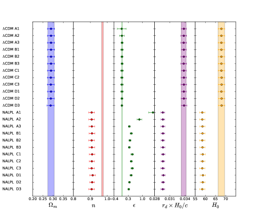
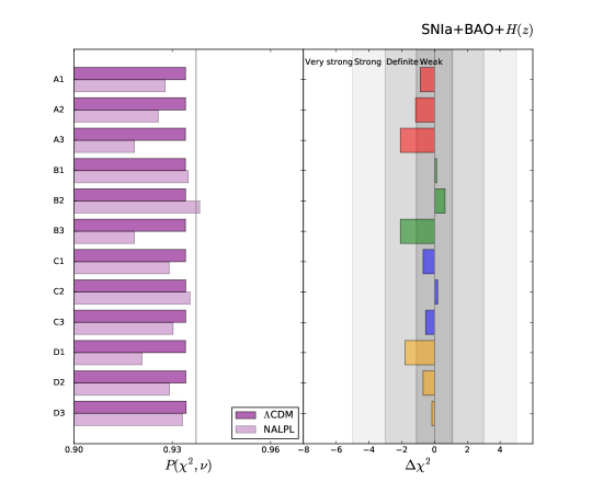
Figure 1: Results obtained from low-redshift background probes. Top panel: Best-fit values for $\Omega_{m}$, $n$, $\epsilon$, $r_{d}\times H_{0}/c,$ and $H_{0}$ parameters for all the cosmological and luminosity evolution models under consideration. The values for these parameters when no luminosity evolution is allowed are represented with bands as a reference. Bottom panel: Goodness of fit statistics and difference of the $\chi^{2}$ values, $\Delta\chi^{2}=\chi^{2}_{\Lambda\text{CDM}}-\chi^{2}_{\text{NALPL}}$, for the luminosity evolution models under study. The vertical solid line in the left plot illustrates the goodness of fit statistics for the standard $\Lambda$CDM imposing no luminosity evolution. The various gray bands in the right plot show the strength of $\Delta\chi^{2}$ given by the Jeffrey scale (see the text for details).

In this section we review the statistical tool used to determine the ability of a model to fit the cosmological data.

To quantify the goodness of a fit we minimize the $\chi^{2}$ function given by

$$\chi^{2}=(\textbf{u}-\textbf{u}_{\text{data}})^{T}C^{-1}(\textbf{u}-\textbf{u}_{\text{data}})\,,$$ (8)

where u stands for the model prediction, while $\textbf{u}_{\text{data}}$ and $C$ hold for the observables and their covariance matrix, respectively. In order to perform the minimization and find the errors on the parameters, we use the MIGRAD application from the iminuit Python package. This package is the Python implementation of the former MINUIT Fortran code [James & Roos (1975)].

We also compute the probability that a higher value for the $\chi^{2}$ occurs for a fit with $\nu=N-k$ degrees of freedom, where $N$ is the number of data points and $k$ is the number of parameters of the model,

$$P(\chi^{2},\nu)=\frac{\Gamma\left(\frac{\nu}{2},\frac{\chi^{2}}{2}\right)}{\Gamma\left(\frac{\nu}{2}\right)}\,,$$ (9)

where $\Gamma(t,x)$ is the upper incomplete gamma function and $\Gamma(t)=\Gamma(t,0)$ the complete gamma function. We use this value as a goodness of fit statistic. A probability close to 1 indicates that it is likely to obtain higher $\chi^{2}$ values than the minimum found, pointing to a good fit by the model.

When combining probes, we minimize the sum of the individual $\chi^{2}$ functions, i.e., we assume that we are dealing with statistically independent probes. Equation (9) is only valid for $N$ data points coming from $N$ independent random variables with Gaussian distributions. In this work we use the correlations within probes; therefore, our data points no longer come from independent Gaussian random variables. However, it has been shown in Tutusaus et al. (2016), through Monte Carlo simulations, that the impact of the correlations we are dealing with is negligible in Eq. (9).

4 Data samples

In this section we present the low-redshift probes, SNIa, BAO, $H(z),$ and $f\sigma_{8}(z)$, and the specific data samples used in this work.

4.1 Type Ia supernovae

Type Ia supernovae are considered standardizable candles useful to measure cosmological distances and break some degeneracies present in other probes, providing us precise cosmological measurements. The standard observable used in SNIa measurements is the distance modulus,

$$\mu(z)=5\log_{10}\left(\frac{H_{0}}{c}d_{L}(z)\right)\,,$$ (10)

where $d_{L}(z)=(1+z)r(z)$ is the luminosity distance.

The standardization of SNIa is based on empirical observation that they form a homogeneous class whose variability can be characterized by two parameters [Tripp (1998)]: the time stretching of the light curve $(X_{1})$ and the supernova color at maximum brightness $(C)$. In this work we use the joint light-curve analysis for SNIa from Betoule et al. (2014). Given the assumption of the authors that supernovae with identical color, shape, and galactic environment have on average the same intrinsic luminosity for all redshifts, the distance modulus can be expressed as

$$\mu_{\text{obs}}=m_{B}^{*}-(M_{B}-\alpha X_{1}+\beta C)\,,$$ (11)

where $m_{B}^{*}$ corresponds to the observed peak magnitude in the B-band rest-frame and $\alpha$ and $\beta$ are nuisance parameters related to the time stretching and the supernova color, respectively. The $M_{B}$ nuisance parameter takes into account the supernova dependence on host galaxy properties and is given by

$$M_{B}=\left\{\begin{array}[]{cl}M_{B}^{1}\,,&\text{if}\,\,M_{\text{stellar}}<10^{10}M_{\odot}\,,\\ M_{B}^{1}+\Delta M\,,&\text{otherwise}\,,\end{array}\right.$$ (12)

where $M_{b}^{1}$ and $\Delta M$ are two extra nuisance parameters.

Concerning the errors and correlations of the measurements, we use the covariance matrix provided in Betoule et al. (2014), where several statistical and systematic uncertainties have been considered, such as the error propagation of the light-curve fit uncertainties, calibration, light-curve model, bias correction, mass step, dust extinction, peculiar velocities, and contamination of non-type Ia supernovae. It is important to stress that this covariance matrix depends on the $\alpha$ and $\beta$ nuisance parameters; therefore, when performing a minimization we recompute the covariance matrix at each step.

Since we do not assume that the intrinsic luminosity of SNIa is independent of the redshift, we consider an extra nuisance term, $\Delta m_{\text{evo}}(z)$, accounting for a possible evolution of the supernovae luminosity with the redshift,

$$\mu_{\text{obs}}=m_{B}^{*}-(M_{B}-\alpha X_{1}+\beta C+\Delta m_{\text{evo}}(z))\,.$$ (13)

Different phenomenological models for $\Delta m_{\text{evo}}(z)$ can be found in the literature [see for example Drell et al. (2000); Linder (2006); Nordin et al. (2008); Ferramacho et al. (2009); Linden et al. (2009)]. In the absence of any clear physics governing this evolution, one stays at a phenomenological level and considers a bunch of different models. We can embed all the models studied in this paper into four categories, which are summarized in table 1. These categories all possess two parameters, $\epsilon$ and $\delta$.

Model B is equivalent to model 2 in Linden et al. (2009), while model C is a generalization of model 1 in Linden et al. (2009). Model D is a generalization of Ferramacho et al. (2009). Models C and D were initially motivated from a parameterization of the intrinsic luminosity $\mathcal{L}\rightarrow\mathcal{L}(1+z)^{-\epsilon}$ [Drell et al. (2000)], while models A and B are more general to study the contribution of powers in $z$ to the results.

Table 1: Different evolution models for SNIa considered in this paper. All models have two different parameters, $\epsilon$ and $\delta$.

Model	$\Delta m_{\text{evo}}(z)$	Reference
A	$\epsilon\left[(1+z)^{\delta}-1\right]$	-
B	$\epsilon z^{\delta}$	Linden et al. (2009)
C	$\epsilon\left[\ln(1+z)\right]^{\delta}$	Linden et al. (2009)
D	$\displaystyle\epsilon\left(\frac{t_{0}-t(z)}{t_{0}-t(1)}\right)^{\delta}$	Ferramacho et al. (2009)

Let us observe that when $\delta\rightarrow 0$, $\Delta m_{\text{evo}}(z)$ becomes strongly degenerate with $M_{B}^{1}$. Therefore, to avoid these kinds of parameter degeneracies, we consider three submodels fixing $\delta=0.3,\,0.5,$ and $1$. We denote these submodels A1, A2, A3, B1, B2, B3, and so on. A lower $\delta$ power contribution models a luminosity evolution dominant at low redshift, while a higher $\delta$ power contribution leads to a luminosity evolution dominating at high redshift.

When using SNIa data, the set of nuisance parameters considered is $\{\alpha,\,\beta,\,M_{B}^{1},\,\Delta M,\epsilon\}$. We consider $\Omega_{m}$ and $n$ as cosmological parameters for the $\Lambda$CDM and the NALPL model, respectively.

4.2 Baryonic acoustic oscillations

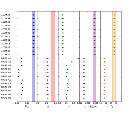
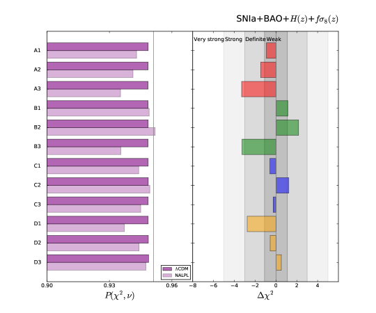
Figure 2: Results obtained from low-redshift background probes combined with measurements of the growth of matter perturbations. Top panel: Best-fit values for $\Omega_{m}$, $n$, $\epsilon$, $r_{d}\times H_{0}/c$, and $H_{0}$ parameters for all the cosmological and luminosity evolution models under consideration. The values for these parameters when no luminosity evolution is allowed are represented with bands as a reference. Bottom panel: Goodness of fit and $\Delta\chi^{2}=\chi^{2}_{\Lambda\text{CDM}}-\chi^{2}_{\text{NALPL}}$ values for the luminosity evolution models under study (see Fig. 1).

The baryonic acoustic oscillations are the regular and periodic fluctuations of visible matter density in large-scale structure. They are characterized by the length of a standard ruler, generally denoted by $r_{d}$. In the $\Lambda$CDM model, the BAO come from sound waves propagating in the early Universe and $r_{d}$ is equal to the comoving sound horizon at the redshift of the baryon drag epoch,

$$r_{d}=r_{s}(z_{d})=\int_{z_{d}}^{\infty}\frac{c_{s}(z)\,\text{d}z}{H(z)}\,,$$ (14)

where $z_{d}\approx 1060$ and $c_{s}(z)$ is the sound velocity as a function of the redshift. Verde et al. (2017) have shown that models differing from $\Lambda$CDM may have a value for $r_{d}$ that is not compatible with $r_{s}(z_{d})$. Moreover, the integral in Eq. (14) is divergent for $n\geq 2/3$ power law cosmologies. According to this, and in order not to delve into early Universe physics, we consider $r_{d}$ as a free parameter.

In this work we use isotropic and anisotropic measurements of the BAO. The distance scale used for isotropic measurements is given by

$$D_{V}(z)\equiv\left(r^{2}(z)\frac{cz}{H(z)}\right)^{1/3}\,,$$ (15)

while for the radial and transverse measurements of the anisotropic BAO the distance scales are $r(z)$ and $c/H(z)$, respectively.

We use the values provided by 6dFGS [Beutler et al. (2011)], SDSS - MGS [Ross et al. (2015)], BOSS - CMASS, and LOWZ samples DR11 [Anderson et al. (2014); Tojeiro et al. (2014)] and BOSS - Ly$\alpha$ forest DR11 [Delubac et al. (2015); Font-Ribera et al. (2014)]. We consider a correlation coefficient of $0.52$ for the CMASS measurements and of $-0.48$ for the Ly-$\alpha$ measurements, while we assume the rest of the measurements to be uncorrelated. In order to take into account the non-Gaussianity of the BAO observable likelihoods far from the peak, we follow Bassett & Afshordi (2010) by replacing the usual $\Delta\chi^{2}_{G}=-2\ln\mathcal{L}_{G}$ for a Gaussian-likelihood observable by

$$\Delta\chi^{2}=\frac{\Delta\chi^{2}_{G}}{\sqrt{1+\Delta\chi^{4}_{G}\left(\frac{S}{N}\right)^{-4}}}\,,$$ (16)

where $S/N$ is the detection significance, in units of $\sigma$, of the BAO feature. We follow Tutusaus et al. (2016) in considering a detection significance of $2.4\sigma$ for 6dFGS, $2\sigma$ for SDSS-MGS, $4\sigma$ for BOSS-LOWZ, $6\sigma$ for BOSS-CMASS, and $4\sigma$ for BOSS-Ly-$\alpha$ forest.

When using BAO data, we add the following parameters to our set: $\{r_{d}\times H_{0}/c,\,\Omega_{m},\,n\}$. The latter two only apply for the $\Lambda$CDM model and NALPL model, respectively. No nuisance parameters are added.

4.3 Hubble parameter $H(z)$

There are two main methods to measure the evolution of the Hubble parameter with respect to the redshift: the so-called differential age method [Jimenez & Loeb (2002)] and a direct measure of $H(z)$ using radial BAO information [Gaztañaga et al. (2009)]. A detailed discussion on the systematic uncertainties of these methods can be found in Zhang & Ma (2010). In this work we use the compilation of independent $H(z)$ measurements from Simon et al. (2005); Stern et al. (2010); Moresco et al. (2012); Busca et al. (2013); Zhang et al. (2014); Blake et al. (2012); Chuang & Wang (2013) provided in Farooq & Ratra (2013). When using $H(z)$ measurements, we add the $H_{0}$ parameter to our set of cosmological parameters under consideration. No nuisance parameters are added.

4.4 Growth rate

The measurements of the growth rate of matter perturbations offer an additional constraint on cosmological models. Their value depends on the theory of gravity used and it is well known that identical background evolution can lead to differente growth rates [Piazza et al. (2014)]. Let us first define the linear growth factor of matter perturbations as the ratio between the linear density perturbation and the energy density,

$$D\equiv\delta\rho_{m}/\rho_{m}\,.$$ (17)

We can then derive the standard second order differential equation for the linear growth factor [Peebles (1993)]

$$\ddot{D}+2H\dot{D}-4\pi G\rho_{m}D=0\,,$$ (18)

where the dot stands for differentitation over the cosmic time. Neglecting second order corrections, this differential equation can be rewritten with derivatives over the scale factor [Dodelson (2003)]

$$D^{\prime\prime}(a)+\left[\frac{3}{a}+\frac{H^{\prime}(a)}{H(a)}\right]D^{\prime}(a)-\frac{3}{2}\Omega_{m}\frac{H_{0}^{2}}{H^{2}(a)}\frac{D(a)}{a^{5}}=0\,.$$ (19)

This expression is only valid if we assume that dark energy cannot be perturbated and does not interact with dark matter. Once we obtained $D$ by solving numerically Eq. (19), we can compute the growth rate as

$$f\equiv\frac{\text{d}\ln D}{\text{d}\ln a}\,,$$ (20)

and the observable weighted growth rate, $f\sigma_{8}$, as

$$f\sigma_{8}(z)=f(z)(K\cdot D(z))\,,$$ (21)

where $K$ is a normalization factor accounting for the root mean square mass fluctuation amplitude on scales of $8h^{-1}$Mpc at redshift $z=0$, $\sigma_{8}$, and the normalization of the growth factor. We do not use the observed value for $\sigma_{8}$ since it requires some assumptions about the early Universe physics. Instead, we let the low-redshift observations choose the preferred value for this normalization.

In this work we use the measurements of $f\sigma_{8}(z)$ from Beutler et al. (2012); Samushia et al. (2012); Tojeiro et al. (2012); Blake et al. (2012); de la Torre et al. (2013) provided in Macaulay et al. (2013), together with their correlations. When using these measurements we add the $K$ parameter and $\Omega_{m}$, for the NALPL model, to our set of parameters under consideration.

5 Results

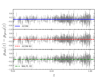
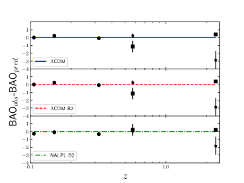
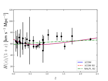
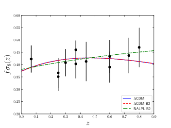
Figure 3: Model predictions vs. observations for the best luminosity evolution model, $\Lambda$CDM B2 and NALPL B2 (together with the standard $\Lambda$CDM prediction, for illustrative purposes) for all the cosmological probes considered. In each prediction, we used the best-fit values obtained from the global fit. Top left: Residuals of SNIa data with respect to the corresponding model. Top right: Residuals of BAO data with respect to the corresponding model. The isotropic measurements of the BAO are represented with a circle and their observable is $D_{V}(z)/r_{d}$, while the stars stand for the radial measurements with observable $r(z)/r_{d}$ and the squares stand for the transverse measurements with observable $c/(H(z)r_{d})$. Bottom left: Measurements of $H(z)/(1+z)$ together with the model predictions. Bottom right: Measurements of $f\sigma_{8}(z)$ and the different model predictions.

We present the results of this work in two different steps. In the first place we focus on low-redshift background probes, namely SNIa, BAO, and $H(z)$, and in the second step we add the measurements of the growth of matter perturbations.

The results obtained from low-redshift background probes only are presented in Fig. 1. In the top panel we show the best-fit values obtained for the $\Omega_{m}$, $n$, $r_{d}\times H_{0}/c$ and $H_{0}$ cosmological parameters, as well as the $\epsilon$ nuisance parameter for the different cosmological and luminosity evolution models under study. The blue region of the left panel corresponds to the value, and the error, obtained for $\Omega_{m}$ in the standard $\Lambda$CDM case, i.e., with no luminosity evolution. We can observe that all the obtained values for $\Omega_{m}$ are completely compatible with the standard $\Lambda$CDM value.

In the second panel we plot the exponent $n$ of NALPL for each model, together with a colored band corresponding to the allowed values when no evolution is imposed. We can observe that all the obtained values are compatible with a slightly lower value than in the no evolution case.

In the third panel we present the nuisance parameter associated with the luminosity evolution for all the models under consideration. As expected, all the $\Lambda$CDM models are perfectly compatible with 0. On the contrary, the NALPL models clearly need some positive luminosity evolution to fit the data.

Concerning the $r_{d}\times H_{0}/c$ cosmological parameter, we can observe that the $\Lambda$CDM values are compatible with the no evolution case, while the values obtained for the NALPL models are compatible with a lower value. This is also the case for the $H_{0}$ parameter, as we can see in the last panel.

Focusing on the ability of these models to fit the data, all of them provide a very good fit to the data with a goodness of fit statistic value of $P(\chi^{2},\nu)>0.9$, as we can see in the left plot of the bottom panel of Fig. 1. We present the difference of $\chi^{2}$ values given by $\Delta\chi^{2}=\chi^{2}_{\Lambda\text{CDM}}-\chi^{2}_{\text{NALPL}}$ in the right plot of Fig. 1 bottom panel. It is important to notice that, in this case, $\Delta\chi^{2}$ is equal to the difference of widely used standard model comparison criteria, such as the Akaike information criterion [Akaike (1973)] or the Bayesian information criterion [Schwarz (1978)], because both $\Lambda$CDM and NALPL have the same number of free parameters and we are using the same data for the fits. However, we are only interested in the ability of NALPL to fit the data, and we are not in search of performing a model comparison against $\Lambda$CDM. In the plot we also show the standard Jeffrey scale [Nesseris & García-Bellido (2013)] to provide a qualitative idea of the strength of the $\Delta\chi^{2}$ variation. We consider $0\leq\Delta\chi^{2}<1.1$ as a weak variation (thus compatible $\chi^{2}$ values), $1.1\leq\Delta\chi^{2}<3$ as a definite variation, $3\leq\Delta\chi^{2}<5$ as a strong variation, and $5\leq\Delta\chi^{2}$ as a very strong variation.

From these results, we can observe that most NALPL models (A1, B1, B2, C1, C2, C3, D2, and D3) are not only able to fit the data with a very high goodness of fit statistic, but their $\chi^{2}$ value is also compatible with that obtained for $\Lambda$CDM.

In Fig. 2 we present the results obtained when adding the measurements of the growth of matter perturbations to the low-redshift background probes. In the top panel we show the best-fit values for the cosmological and nuisance parameters. The obtained values for the $\Lambda$CDM models are completely compatible with the no luminosity evolution case, as in the previous case (Fig. 1). The only difference here are slightly smaller error bars due to the introduction of more data points. Concerning the NALPL models, we have an extra cosmological parameter, $\Omega_{m}$, which is very well constrained, but the other parameters remain qualitatively compatible with the results from Fig. 1: the cosmological parameters $n$, $r_{d}\times H_{0}/c$ and $H_{0}$ are compatible with lower values than for the no luminosity evolution case, while $\epsilon$ is clearly not compatible with 0.

In the bottom panel of Fig. 2 we provide the results for the goodness of fit statistic and the variation of the $\chi^{2}$ values. In the first plot we can observe that all models provide a very good fit to the data ($P(\chi^{2},\nu)>0.93$), while in the second panel we show that most NALPL models (A1, B1, B2, C1, C2, C3, D2, and D3) have a $\chi^{2}$ value compatible with (or slightly better than) those provided by $\Lambda$CDM. From a model criteria point of view it is clear that NALPL is slightly disfavored because of the introduction of the extra $\Omega_{m}$ parameter. However, the importance of the Occam factor depends on the model criteria used and, as discussed before, our goal is not to test the NALPL model against $\Lambda$CDM to adopt this model as an alternative, but just to show that it can fit the observational data extremely well.

In Fig. 3, just for completeness and illustrative purposes, we present the prediction for all probes using the best low-redshift power law model (B2), $\Lambda$CDM B2, and $\Lambda$CDM imposing no luminosity evolution. We used the global best-fit values for the cosmological and nuisance parameters. It is clear that all three models are able to reproduce the observations extremely well.

Taking all the low-redshift probes into account (SNIa, BAO, $H(z),$ and $f\sigma_{8}(z)$), a NALPL model is perfectly compatible with the data for several luminosity evolution models. This points to the fact that low-redshift probes do not definitively prove the acceleration of the Universe and that we need more precise low-redshift measurements to claim this acceleration firmly.

6 Conclusions

In this work we have analyzed the ability of the low-redshift probes (SNIa, BAO, $H(z)$, and $f\sigma_{8}(z)$) to prove the accelerated expansion of the Universe. More precisely, we considered a nonaccelerating low-redshift power law cosmology and checked its ability to fit these cosmological data. Using only the low-redshift background probes, and not imposing the SNIa intrinsic luminosity to be redshift independent (accounting for several luminosity evolution models), we find that a nonaccelerated low-redshift power law cosmology is able to fit very well all the observations, for all the luminosity evolution models considered. Moreover, most of the NALPL models provide a value for the $\chi^{2}$ perfectly compatible with that obtained for $\Lambda$CDM.

When we add the measurements of the growth of matter perturbations, a nonaccelerated low-redshift power law cosmology is able to fit all the data extremely well for all the luminosity evolution models considered. As in the previous case, most of the NALPL models provide $\chi^{2}$ values that are perfectly compatible (or even slightly better) than those coming from $\Lambda$CDM.

The main conclusion of this work is that if we do not impose the SNIa intrinsic luminosity to be independent of the redshift, the combination of low-redshift probes is not sufficient to firmly prove the accelerated expansion of the Universe.

References

- Akaike (1973) Akaike, H. 1973, Proc. Second International Symposium on Information Theory, eds. B. N. Petrov, & F. Caski (Akademiai Kiado, Budapest), 267
- Anderson et al. (2014) Anderson, L., Aubourg, E., Bailey, S., et al. 2014, MNRAS, 441, 24
- Bassett & Afshordi (2010) Bassett, B. A. & Afshordi, N. 2010, ArXiv e-prints [arXiv:1005.1664]
- Betoule et al. (2014) Betoule, M., Kessler, R., Guy, J., et al. 2014, A&A, 568, A22
- Beutler et al. (2011) Beutler, F., Blake, C., Colless, M., et al. 2011, MNRAS, 416, 3017
- Beutler et al. (2012) Beutler, F., Blake, C., Colless, M., et al. 2012, MNRAS, 423, 3430
- Blake et al. (2012) Blake, C., Brough, S., Colless, M., et al. 2012, MNRAS, 425, 405
- Busca et al. (2013) Busca, N. G., Delubac, T., Rich, J., et al. 2013, A&A, 552, A96
- Chuang & Wang (2013) Chuang, C.-H. & Wang, Y. 2013, MNRAS, 435, 255
- de la Torre et al. (2013) de la Torre, S., Guzzo, L., Peacock, J. A., et al. 2013, A&A, 557, A54
- Delubac et al. (2015) Delubac, T., Bautista, J. E., Busca, N. G., et al. 2015, A&A, 574, A59
- Dodelson (2003) Dodelson, S. 2003, Modern Cosmology (Amsterdam: Academic Press)
- Dolgov et al. (2014) Dolgov, A., Halenka, V., & Tkachev, I. 2014, J. Cosmol. Astropart. Phys., 10, 047
- Dolgov (1997) Dolgov, A. D. 1997, Phys. Rev. D, 55, 5881
- Drell et al. (2000) Drell, P. S., Loredo, T. J., & Wasserman, I. 2000, ApJ, 530, 593
- Farooq & Ratra (2013) Farooq, O. & Ratra, B. 2013, ApJ, 766, L7
- Ferramacho et al. (2009) Ferramacho, L. D., Blanchard, A., & Zolnierowski, Y. 2009, A&A, 499, 21
- Fixsen (2009) Fixsen, D. J. 2009, ApJ, 707, 916
- Font-Ribera et al. (2014) Font-Ribera, A., Kirkby, D., Busca, N., et al. 2014, J. Cosmol. Astropart. Phys., 05, 027
- Gaztañaga et al. (2009) Gaztañaga, E., Cabré, A., & Hui, L. 2009, MNRAS, 399, 1663
- James & Roos (1975) James, F. & Roos, M. 1975, Comput. Phys. Commun., 10, 343
- Jimenez & Loeb (2002) Jimenez, R. & Loeb, A. 2002, ApJ, 573, 37
- Kaplinghat et al. (1999) Kaplinghat, M., Steigman, G., Tkachev, I., & Walker, T. P. 1999, Phys. Rev. D, 59, 043514
- Kaplinghat et al. (2000) Kaplinghat, M., Steigman, G., & Walker, T. P. 2000, Phys. Rev. D, 61, 103507
- Linden et al. (2009) Linden, S., Virey, J.-M., & Tilquin, A. 2009, A&A, 506, 1095
- Linder (2006) Linder, E. V. 2006, Astropart. Phys., 26, 102
- Macaulay et al. (2013) Macaulay, E., Wehus, I. K., & Eriksen, H. K. 2013, Phys. Rev. Lett., 111, 161301
- Moresco et al. (2012) Moresco, M., Cimatti, A., Jimenez, R., et al. 2012, J. Cosmol. Astropart. Phys., 08, 006
- Nesseris & García-Bellido (2013) Nesseris, S. & García-Bellido, J. 2013, J. Cosmol. Astropart. Phys., 08, 036
- Nielsen et al. (2016) Nielsen, J. T., Guffanti, A., & Sarkar, S. 2016, Nature Sci. Rep., 6, 35596
- Nordin et al. (2008) Nordin, J., Goobar, A., & Jönsson, J. 2008, J. Cosmol. Astropart. Phys., 02, 008
- Peebles (1993) Peebles, J. E. 1993, Principles of Physical Cosmology, Princeton Theories in Physics (Princeton University Press)
- Perlmutter et al. (1999) Perlmutter, S., Aldering, G., Goldhaber, G., et al. 1999, ApJ, 517, 565
- Piazza et al. (2014) Piazza, F., Steigerwald, H., & Marinoni, C. 2014, J. Cosmol. Astropart. Phys., 05, 043
- Planck Collaboration et al. (2016) Planck Collaboration, Ade, P. A. R., Aghanim, N., et al. 2016, A&A, 594, A13
- Rani et al. (2015) Rani, S., Altaibayeva, A., Shahalam, M., Singh, J., & Myrzakulov, R. 2015, J. Cosmol. Astropart. Phys., 03, 031
- Riess et al. (1998) Riess, A. G., Filippenko, A. V., Challis, P., et al. 1998, Astron. J., 116, 1009
- Ringermacher & Mead (2016) Ringermacher, H. I. & Mead, L. R. 2016, ArXiv e-prints [arXiv:1611.00999]
- Ross et al. (2015) Ross, A. J., Samushia, L., Howlett, C., et al. 2015, MNRAS, 449, 835
- Rubin & Hayden (2016) Rubin, D. & Hayden, B. 2016, ApJ, 833, L30
- Samushia et al. (2012) Samushia, L., Percival, W. J., & Raccanelli, A. 2012, MNRAS, 420, 2102
- Schwarz (1978) Schwarz, G. 1978, Ann. Statist., 6, 461
- Shafer (2015) Shafer, D. L. 2015, Phys. Rev. D, 91, 103516
- Shariff et al. (2016) Shariff, H., Jiao, X., Trotta, R., & van Dyk, D. A. 2016, ApJ, 827, 1
- Simon et al. (2005) Simon, J., Verde, L., & Jimenez, R. 2005, Phys. Rev. D, 71, 123001
- Stern et al. (2010) Stern, D., Jimenez, R., Verde, L., Kamionkowski, M., & Stanford, S. A. 2010, J. Cosmol. Astropart. Phys., 02, 008
- Tojeiro et al. (2012) Tojeiro, R., Percival, W. J., Brinkmann, J., et al. 2012, MNRAS, 424, 2339
- Tojeiro et al. (2014) Tojeiro, R., Ross, A. J., Burden, A., et al. 2014, MNRAS, 440, 2222
- Tripp (1998) Tripp, R. 1998, A&A, 331, 815
- Tutusaus et al. (2016) Tutusaus, I., Lamine, B., Blanchard, A., et al. 2016, Phys. Rev. D, 94, 103511
- Verde et al. (2017) Verde, L., Bernal, J. L., Heavens, A. F., & Jimenez, R. 2017, MNRAS, 467, 731
- Zhang et al. (2014) Zhang, C., Zhang, H., Yuan, S., et al. 2014, Res. Astron. Astrophys., 14, 1221
- Zhang & Ma (2010) Zhang, T.-J. & Ma, C. 2010, Adv. Astron., 2010, 184284