Latent Variable Modeling for the Microbiome

Abstract

The human microbiome is a complex ecological system, and describing its structure and function under different environmental conditions is important from both basic scientific and medical perspectives. Viewed through a biostatistical lens, many microbiome analysis goals can be formulated as latent variable modeling problems. However, although probabilistic latent variable models are a cornerstone of modern unsupervised learning, they are rarely applied in the context of microbiome data analysis, in spite of the evolutionary, temporal, and count structure that could be directly incorporated through such models. We explore the application of probabilistic latent variable models to microbiome data, with a focus on Latent Dirichlet Allocation, Nonnegative Matrix Factorization, and Dynamic Unigram models. To develop guidelines for when different methods are appropriate, we perform a simulation study. We further illustrate and compare these techniques using the data of Dethlefsen and Relman (2011), a study on the effects of antibiotics on bacterial community composition. Code and data for all simulations and case studies are available publicly.

1 Introduction

Microbiome studies attempt to characterize variation in bacterial abundance profiles across different experimental conditions (Human Microbiome Project Consortium, 2012; Gilbert and others, 2014). For example, a study may attempt to describe differences in bacterial communities between diseased and healthy states or after deliberately induced perturbations (Dethlefsen and Relman, 2011; Fukuyama and others, 2017).

In the process, two complementary difficulties arise. First, the data are often high-dimensional, measured over several hundreds or thousands types of bacteria. Studying patterns at the level of particular bacteria is typically uninformative. Second, it can be important to study bacterial abundances in the context of existing biological knowledge. For example, it is scientifically meaningful when a collection of bacteria that are known to be evolutionarily related have either similar or opposed abundance profiles. These challenges motivate methodological work in the microbiome, including phylogenetically-informed techniques for dimensionality-reduction and high-dimensional regression.

Towards phylogenetically-informed dimensionality reduction, Chen and others (2013), who applied a structured regularization penalty in sparse CCA to incorporate phylogenetic information, encouraging scores for similar species to be placed close to one another. A similar effect can be obtained by placing an appropriate prior in a Bayesian model, an approach explored in Fukuyama (2017). By varying the strength of the prior, it is possible to encourage different degrees of smoothness with respect to phylogeny, and Empirical Bayes estimation allows for a certain type of adaptivity.

In addition to dimensionality reduction, high-dimensional classification is popular in the microbiome literature. Often interesting species can be identified by searching for important features in models that predict sample characteristics – treatment vs. control, for example – from species abundances. Segata and others (2011) provided an approach for accounting for phylogenetic structure in this problem by initially prescreening according to independent biological interest. Alternatively, Chen and Li (2013) applied a Dirichlet Multinomial regression model to study the relationship between bacterial counts and sample characteristics in a fully generative fashion, and then added an $\ell^{1}$-penalty to induce sparsity and facilitate interpretability. Shafiei and others (2015) designed a different generative supervised model, based on ideas from mixed-membership modeling (Blei and others, 2003). The development of structured modeling techniques tailored to the microbiome remains an active area of current research.

2 Methods

We review a few of the statistical modeling techniques that are the focus of this work. Many of these techniques have been borrowed from text analysis, thinking of the bacterial counts matrix as a biological analog of the document-term matrix. The idea of transferring these techniques to the microbiome is not new, though its appropriateness and usefulness has only been explored in relatively limited settings (Schloss and Handelsman, 2007; Holmes and others, 2012; Chen and others, 2012; Chen and Li, 2013; Shafiei and others, 2015; Jiang and others, 2017).

2.1 Dirichlet Multinomial Mixture Model

While the multinomial distribution is the fundamental probability mechanism for sampling counts, multinomial models are only appropriate for relatively homogeneous data sets, where categories are nearly independent. An extension, Dirichlet multinomial mixture modeling, allows for count modeling in the presence of increased heterogeneity, and its relevance to the text and microbiome settings were key contributions of Nigam and others (2000) and Holmes and others (2012), respectively. In this section, we adopt text analysis terminology, where the count matrices of interest are counts of terms across documents. In Section 2.6 we clarify the connection to microbiome analysis.

Suppose there are $D$ documents across $V$ terms, and that these documents are assumed to belong to one of $K$ underlying topics, where a topic is defined as a distribution over words. The Dirichlet multinomial mixture model draws each topic from a distribution over probabilities. Then, for each document, a topic is chosen by flipping a $K$-sided coin with probability $\theta_{k}$ of coming up on side $k$. Conditional on the selected topic, all words are drawn independently from the probabilites associated with the selected topic.

More formally, represent the topic for the $d^{th}$ document by $z_{d}\in\{1,\dots,K\}$ and the term in the $n_{th}$ word of this document by $w_{dn}$. Suppose the $k^{th}$ topic places weight $\beta_{vk}$ on the $v^{th}$ term, so that $\beta_{k}\in\mathcal{S}^{V-1}$. Suppose there are $N_{d}$ words in the $d^{th}$ document. Then, the generative mechanism for the observed data set is

$$w_{dn}|\left(\beta_{k}\right)_{k=1}^{K},z_{d} \overset{iid}{\sim}\textnormal{Mult}\left(1,\beta_{z_{d}}\right)\text{ for }d=1,\dots,D\text{ and }n=1,\dots,N_{d}$$

$$z_{d}|\theta \overset{iid}{\sim}\textnormal{Mult}\left(1,\theta\right)\text{ for }d=1,\dots,D$$

$$\beta_{k} \overset{iid}{\sim}\textnormal{Dir}\left(\gamma\right)\text{ for }k=1,\dots,K.$$

Equivalently, we could write $w_{d}|\left(\beta_{k}\right)_{k=1}^{K},z_{d}\sim\textnormal{Mult}\left(N_{d},\beta_{z_{d}}\right)$, though the form above makes comparison with LDA more straightforward. Further, while we treat $\theta$, and $\gamma$ as fixed parameters, it is possible to place priors on them as well. Geometrically, this model identifies each document with one of the $\beta_{k}$ on the $V$-dimensional simplex.

In practice, interpretation revolves around the posterior topic memberships, $\mathbb{P}\left({z_{d}=k|\left(w_{dn}\right)}\right)$, and probabilities, $\mathbb{P}\left({\beta_{kv}|\left(w_{dn}\right)}\right)$. While these estimates can be useful in guiding scientific analysis (Nigam and others, 2000; Holmes and others, 2012), the assumption that each document belongs completely to one topic is sometimes unnecessarily restrictive. For example, in learning a Dirichlet multinomial mixture model on a collection of newspaper articles, we may recover separate topics related to science and personal health, but there would be no way to express the mixture of topics in an article about health research.

2.2 Latent Dirichlet Allocation

Latent Dirichlet Allocation (LDA) is a generalization of Dirichlet multinomial mixture modeling where documents are allowed to have fractional membership across a set of topics (Blei and others, 2003). This addresses the key limitation of Dirichlet multinomial mixture modeling, and one goal of the case study in Section 4 is to demonstrate the usefulness of this additional flexibility in microbiome analysis.

We use the same notation as before, but instead of fixing a global $\theta$ parameter, let $\theta_{d}\in\mathcal{S}^{K-1}$ represent the $d^{th}$ document’s mixture over the $K$ underlying topics. Represent the term in the $n_{th}$ word of this document by $w_{dn}$, and the associated topic by $z_{dn}$. Suppose the $k^{th}$ topic places weight $\beta_{vk}$ on the $v^{th}$ term, so that $\beta_{k}\in\mathcal{S}^{V-1}$. Suppose there are $N_{d}$ words in the $d^{th}$ document. Then, the generative mechanism for the observed data set is

$$w_{dn}|\left(\beta_{k}\right)_{k=1}^{K},z_{dn} \overset{iid}{\sim}\textnormal{Mult}\left(1,\beta_{z_{dn}}\right)\text{ for }d=1,\dots,D\text{ and }n=1,\dots,N_{d}$$

$$z_{dn}|\theta_{d} \overset{iid}{\sim}\textnormal{Mult}\left(1,\theta_{d}\right)\text{ for }d=1,\dots,D\text{ and }n=1,\dots,N_{d}$$

$$\theta_{d} \overset{iid}{\sim}\textnormal{Dir}\left(\alpha\right)\text{ for }d=1,\dots,D$$

$$\beta_{k} \overset{iid}{\sim}\textnormal{Dir}\left(\gamma\right)\text{ for }k=1,\dots,K.$$

In microbiome applications, we will find a formulation that marginalizes over the $z_{dn}$ more convenient. Setting $x_{dv}=\sum_{n=1}^{N_{d}}\mathbb{I}\left({w_{dn}=v}\right)$, we can write the marginal distribution as

$$x_{d\cdot}|\left(\beta_{k}\right)_{1}^{K} \overset{iid}{\sim}\textnormal{Mult}\left(N_{d},B\theta_{d}\right)\text{ for }d=1,\dots,D$$

$$\theta_{d} \overset{iid}{\sim}\textnormal{Dir}\left(\alpha\right)\text{ for }d=1,\dots,D$$

$$\beta_{k} \overset{iid}{\sim}\textnormal{Dir}\left(\gamma\right)\text{ for }k=1,\dots,K,$$

where we have introduced the $V\times K$ matrix concatenating all topics column-wise, $B=\begin{pmatrix}\beta_{1},\dots,\beta_{K}\end{pmatrix}$. Geometrically, LDA identifies samples with points in the convex hull of $K$ topics $\left(\beta_{k}\right)$ on the $V$-dimensional simplex, rather than the individual corners, as in the Dirichlet multinomial mixture model.

2.3 Dynamic Unigram model

Upon examining this geometric interpretation, we might consider in some situations a model that identifies samples with a continuous curve on this $V$-dimensional simplex. This reasoning leads naturally to the Dynamic Unigram model (Blei and Lafferty, 2006). The underlying curve reflects the gradual evolution of probabilities over time, and is implemented by passing a random walk through a multilogit link. That is, the Dynamic Unigram model posits the generative model

$$x_{d\cdot}|\mu_{t\left(d\right)} \overset{iid}{\sim}\textnormal{Mult}\left(N_{d},S\left(\mu_{t\left(d\right)}\right)\right)\text{ for }d=1,\dots,D$$

$$\mu_{t}|\mu_{t-1} \overset{iid}{\sim}\mathcal{N}\left(\mu_{t-1},\sigma^{2}I_{V}\right)\text{ for }t=1,\dots,T$$

$$\mu_{0} \overset{iid}{\sim}\mathcal{N}\left(0,\sigma^{2}I_{V}\right),$$

where $S$ is the multilogit link

$$\left[S\left(\mu\right)\right]_{v}=\frac{\operatorname{exp}\left(\mu_{v}\right)}{\sum_{v^{\prime}}\operatorname{exp}\left(\mu_{v^{\prime}}\right)},$$

and $t\left(d\right)$ maps document $d$ to the time it was sampled. The $\left(\mu_{t\left(\right)}\right)$ define a Gaussian random walk in $\mathbb{R}^{V}$ with step-size $\sigma$, and $S$ transforms the walk into a sequence of probability distributions. In our experiments, we place a vague inverse-gamma prior on $\sigma^{2}$, since this hyperparameter is rarely known in practice.

2.4 Nonnegative Matrix Factorization

In LDA, count matrices are modeled by sampling from multinomials with total counts coming from the word count of each document and probabilities coming from the rows of $\Theta B^{T}$ where $\Theta=\begin{pmatrix}\theta_{1}\\ \vdots\\ \theta_{D}\end{pmatrix}$ and $B=\begin{pmatrix}\beta_{1}\dots\beta_{K}\end{pmatrix}$ are $D\times K$ and $V\times K$ matrices representing document and topic distributions, respectively, and where each $\theta_{d}\in\mathcal{S}^{K-1}$ and $\beta_{k}\in\mathcal{S}^{V-1}$.

Alternatively, it is possible to model the nonnegative matrix $X$ by the product of low rank matrices, $X\approx\Theta B^{T}$, where now the only constraints on $\Theta$ and $B$ are that $\Theta\in\mathbb{R}_{+}^{D\times K}$ and $B\in\mathbb{R}_{+}^{V\times K}$. This is the point of departure for a variety of algorithms in the Nonnegative Matrix Factorization (NMF) literature (Wang and Zhang, 2013; Berry and others, 2007; Lee and Seung, 2001)

We focus on the Gamma-Poisson factorization model (GaP) (Kucukelbir and others, 2015; Carpenter and others, 2016; Zhou and Carin, 2015; Canny, 2004) which posits the hierarchical model

$$X \sim\textnormal{Poi}\left(\Theta B^{T}\right)$$

$$\Theta \sim\textnormal{Gam}\left(a_{0}1_{D\times K},b_{0}1_{D\times K}\right)$$

$$B \sim\textnormal{Gam}\left(c_{0}1_{V\times K},d_{0}1_{V\times K}\right),$$

where our notation means that each entry in these matrices is sampled independently, with parameters given by the corresponding entry in the parameter matrix. As a consequence of the representation of the negative binomial distribution as a Gamma mixture of Poissons, this is a natural model of overdispersed counts, which arise frequently in genomic and microbiome settings (Love and others, 2014; McMurdie and Holmes, 2014). In practice, the hyperparameters $a_{0},b_{0},c_{0}$, and $d_{0}$ are unknown. In all of our experiments, we optimize over them, though it would also be possible to add a level to the hierarchy and place vague nonnegative priors on these parameters.

In our simulation studies, we also consider a slight variant of this model, similar to the proposal of (Romero and others, 2014), which independently sends entries of $X$ to zero with probability $p_{0}$. In our experiments, we assume that this zero-inflation probability is known. This procedure is denoted by Z-NMF.

2.5 Posterior Predictive Checks

Model assessment is important for qualifying interpretations, and can further guide refinements in subsequent analyses. Indeed, part of the appeal of probabilistic modeling is the ease with which models can be adapted to better describe the data of interest. We briefly review model assessment via posterior predictive checks (Rubin and others, 1984; Gelman and Shalizi, 2013), as they are applied in Section 4.3. In this approach, some statistics $T_{k}\left(x\right)$ of the data are defined which, in some sense, “characterize” the data. If the data $x^{\ast}$ simulated from the fitted model have statistics $T_{k}\left(x^{\ast}\right)$ with values similar to those in the observed data $T_{k}\left(x\right)$, then we have evidence that the proposed model approximates the data well, at least in the sense defined by $T_{k}$.

More precisely, simulate data $x_{1}^{\ast},\dots,x_{S}^{\ast}$ from the posterior predictive probability distribution $p\left(x^{\ast}|x\right)\approx\int p\left(x^{\ast}|\theta\right)\hat{p}\left(\theta|x\right)d\theta$, where $x$ is the original data and $\hat{p}\left(\theta|x\right)$ is an estimate of the posterior. For each of these simulated data sets, the characterizing statistics $T_{k}\left(x_{s}\right)$ are computed. Graphically comparing the $T_{k}\left(x\right)$ calculated on the true data with the histogram of model-fit simulated $T_{k}\left(x_{s}^{\ast}\right)$ suggests ways in which the posited model fits – the case where the observed $T_{k}\left(x\right)$ lie in the bulk of the $T_{k}\left(x^{\ast}_{s}\right)$ – or fails to fit – the case where $T_{k}\left(x\right)$ lie far from the bulk of $T_{k}\left(x^{\ast}_{s}\right)$ – the data well.

For example, it is common to set $T_{k}\left(x\right)=\overline{x}_{d}$ or $\frac{1}{n}\sum_{i}\left(x_{id}-\overline{x}_{d}\right)^{2}$ to see whether simulated samples approximately match the moments of the $d^{th}$ dimension in the observed data. Alternatively, histograms of raw data or raw data subsetted to certain groups can guide evaluation. This corresponds to setting a multidimensional $T_{k}\left(x\right)$. For example, $T_{k}\left(x_{s}^{\ast}\right)=\left(n_{s1},\dots,n_{sB}\right)$ could count the number of observations in the $s^{th}$ simulated data set falling into histogram bins $b=1,\dots,B$.

2.6 Microbiome vs. Text Analysis

One of the primary contributions of our work is to develop the observation that methods popular in text analysis can be adapted to the microbiome setting in a way that produces useful summaries. Before applying these methods, we develop the analogy between these text and microbiome analysis and also draw attention to points where the parallels break down.

In the abstract, it becomes clear that the semantic differences between the units of statistical analysis are often superficial. For example, we can map between the most common field-specific terms as follows,

• Document $\iff$ Biological Sample: The basic sampling units, over which conclusions are generalized, are documents (text analysis) and biological samples (microbiome analysis). It is of interest to highlight similarities and differences across these units, often through some variation on clustering or dimensionality reduction.

• Term $\iff$ Bacterial species: The fundamental features with which to describe samples are the counts of terms (text analysis) and bacterial species (microbiome analysis). More formally, by bacterial species, we mean Amplicon Sequence Variants (Callahan and others, 2017), though we avoid this terminology for simplicity of exposition.

• Topic $\iff$ Community: For interpretation, it is common to imagine “prototypical” units which can be used as a point of reference for observed samples. In text analysis, these are called topics – for example, “business” or “politics” articles have their own specific vocabularies. On the other hand, in microbiome analysis, these are called “communities” – different communities have different bacterial signatures.

• Word $\iff$ Sequencing Read: A “word” in text analysis refers to a single instance of a term in a document, not its total count. The analog in microbiome analysis is an individual read that has been mapped to a unique sequence variant, though this is rarely an object of intrinsic interest.

• Corpus $\iff$ Environment: Sometimes a grouping structure is known apriori among sampling units. In this case, it can be informative to describe whether topics are or are not shared across these groups (Teh and others, 2004). In the text analysis literature, a known group of documents – for example, all articles coming from one newspaper – is called a corpus. In the microbiome literature, the associated concept is the environment – for example, skin, ocean, or soil – from which a sample was obtained.

Now that we have established the semantic connections between text and microbiome analysis, we compare the types of data and analysis goals that are typical within the respective fields. In both, a central element of study is the sample-by-feature (either document-by-term or biological sample-by-bacteria) matrix. Besides count structure, the most striking similarity between these data matrices is sparsity: most entries are zero. Further, observed counts tend to be highly-skewed – some terms are far more common than others, and in the same way, some microbes are much more abundant than others. Finally, in both fields, contextual information beyond the raw sample-by-feature matrix is typically available. For example, timestamps are often available in both domains, $n$-grams have a natural analog in terms of small subnetworks of co-occurring bacteria, and phylogenetic similarity between species parallels apriori known linguistic characteristics of terms.

Nonetheless, in practice, the structure of these data can be quite different. First, text data can be on a much larger scale. For example, the Wikipedia corpus studied by Hoffman and others (2013) includes 3.8 million articles. In contrast, even large microbiome datasets, like the one studied in (Gilbert and others, 2014), typically only have on the order of tens of thousands of samples. Similarly, the total number of terms in such large-scale text analysis problems can be substantially larger than the number of bacterial species under consideration.

On the other hand, in a different sense, microbiome studies are larger in scale – there tend to be tens of thousands of reads per sample in microbiome studies, but only hundreds to thousands of words within any article. This means that techniques that rely on the representation of documents as sequences of individual words, rather than vectors of word counts, require too much memory to be practical. This makes many useful text analysis techniques – for example, some methods for model inference (Griffiths and Steyvers, 2004) and evaluation (Wallach and others, 2009) – out of reach for standard microbiome problems. This does, however, suggest potential opportunities for future research.

Lastly, we compare the prevailing analytical goals within text and microbiome analysis. In both fields, data reduction can be informative for developing models of system behavior. However, an essential difference is that even unsupervised text analysis techniques are often embedded within automatic systems, for text classification (Blei and others, 2003) or information retrieval (Krestel and others, 2009) for example, which do not require the intervention of a scientific investigator. In contrast, in microbiome studies, researchers often have control over specific experimental design structure, and collect and analyze data on a per-study basis. In this setting, success is defined somewhat amorphously as an ability to describe the structure and function underlying a biological system of interest.

3 Simulation Study

It can be liberating to have easy access to such a variety of modeling strategies for any given microbiome analysis problem. However, with this increased flexibility comes the difficulty of determining when to use which methods. To build some intuition about estimation accuracy across combinations of data settings and model types, we conduct a series of simulation studies. These are meant to complement the model-checking that should follow parametric analysis – since we know the truth in simulations, it is easier to develop more unambiguous guidelines.

More specifically, our plan is to divide our experiments into simulations generating data from the true LDA, unigram, and NMF / Z-NMF models. In each, we vary the sample size and dimension, performing model estimation using either Markov Chain Monte Carlo (MCMC) sampling, Variational Bayes (VB), or a bootstrap. The only misspecification we consider is a failure to account for zero inflation when the true data were generated according to the Z-NMF model – though not pursued here, it could be interesting to study robustness of study conclusions to misspecification in the number of topics or deliberate contamination.

For the LDA experiment, we vary the number of samples $D\in\{20,100\}$, the number of features $V\in\{325,650\}$, and the total count per sample $N\in\{1625,3250,6500\}$, in order to approximately match dimensions typical in real microbiome datasets. On the other hand, we fix the number of topics to $K=2$ and the Dirichlet hyperparameter to $\alpha=\gamma=1$. For each simulated data set, we perform estimation using MCMC sampling, VB, and a parametric bootstrap. In more detail, this bootstrap procedure fits VB to the original data, simulates $B=500$ new datasets $X^{\ast}_{b}$ according to the LDA model using VB-estimated parameters $\{\hat{\theta}^{\ast}_{b},\hat{\beta}^{\ast}_{b}\}$, and re-estimates parameters $\{\hat{\theta}^{\ast\ast}_{b},\hat{\beta}^{\ast\ast}_{b}\}$ on each simulated data set, again using VB. The motivation for this procedure is the desire to strike an easily-parallelizable compromise between MCMC sampling, which can be time consuming but has reliable uncertainty estimates, and VB, which is fast, but can underestimate uncertainty (Wang and Titterington, 2005).

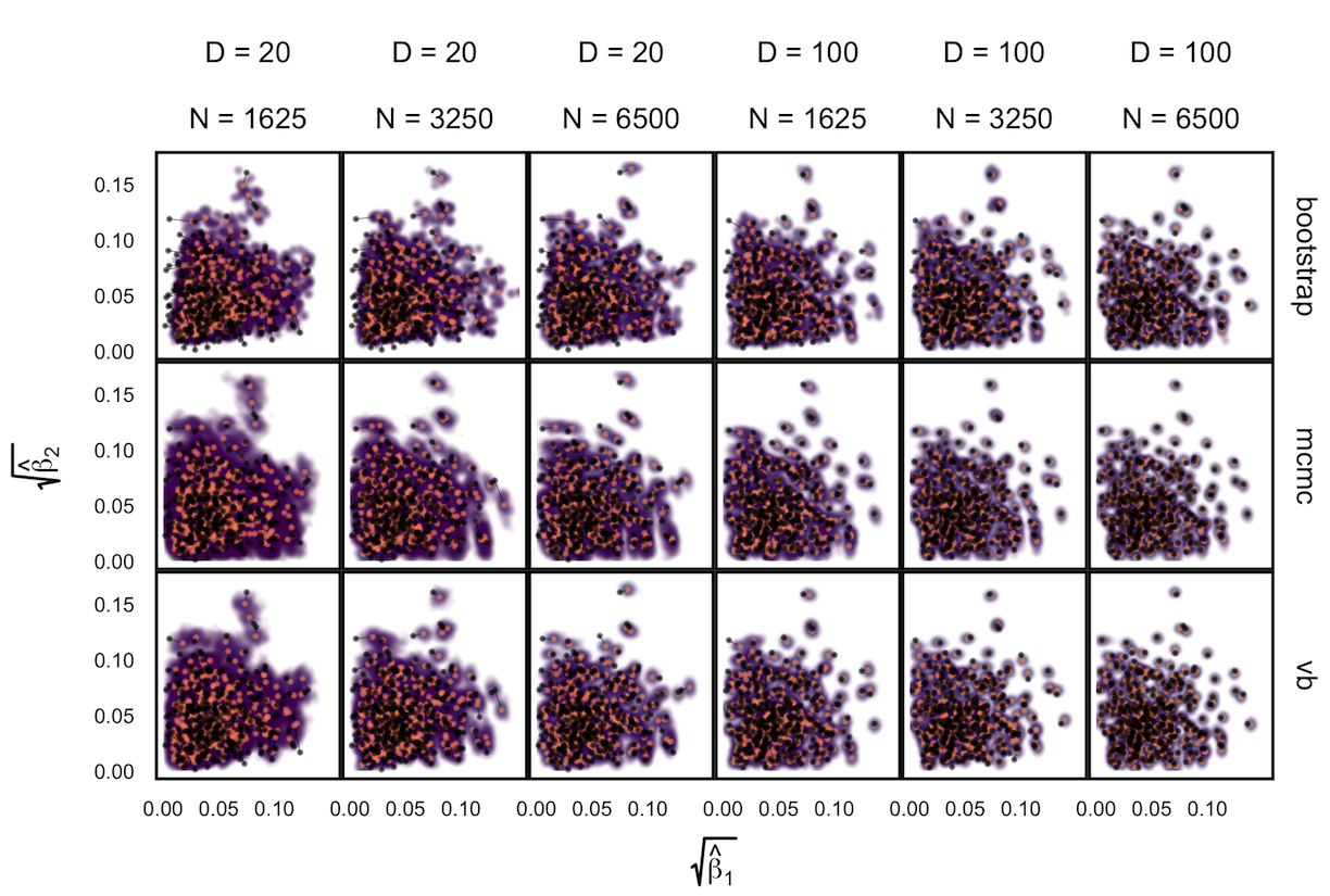
Figure 10: The analog of Figure 1 in the case that $V=325$.

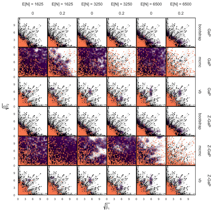
Figure 11: The results of the NMF experiment with $D=20$ Within each panel, we display the true value of $\sqrt{\beta_{v}}$ as black points, while linked orange points give associated posterior medians. Note that the axes are truncated, and for some panels, the posterior medians all lie outside the visible box. Across columns, we vary and $\mathbb{E}\left[{N}\right]$. Along rows, we vary the assumed model, the inference procedure, and the true $p_{0}$ – these are the three columns of row labels, read from outside in.

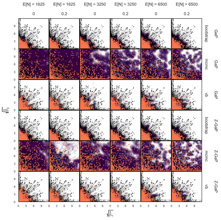
Figure 12: The analog of Figure 11 when $D=100$.

Note that, due to the label-switching problem, it is not possible to directly compare the estimated topics across simulation configurations. To address this issue, we attempt to identify the permutation that aligns topics across all experiments. For each experiment, we identify the true-estimated topics pair with highest correlation, then find the next highest pair among the remaining, and so forth. Judging from the aligned densities in Figure 1 and Supplementary Figures 10, 11, and 12, this ad-hoc alignment procedure seems sufficient.

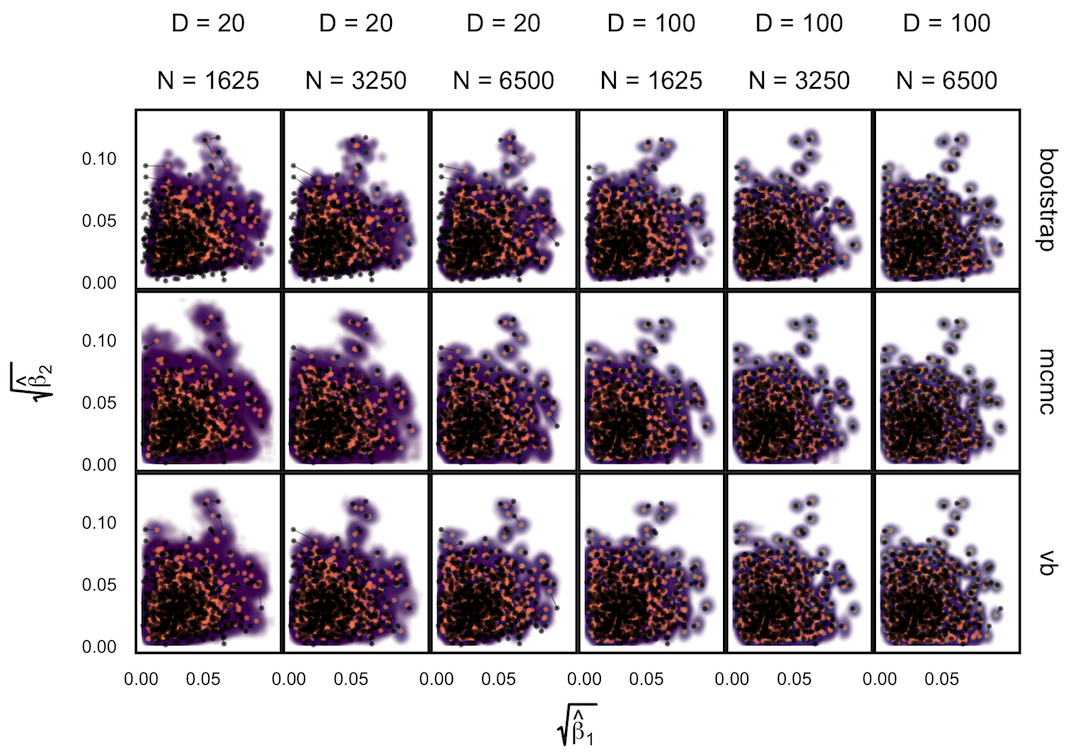
Figure 1: Different inference algorithms for LDA provide comparable posterior estimates under the simulation configurations we have considered. Within each panel, we display the true pairs $\left(\sqrt{\beta_{v1}},\sqrt{\beta_{v2}}\right)$ as black points $v$. The purple clouds are posterior samples from the inference procedure, which are given as row labels. The posterior medians are orange points that are linked to the true $v$. Different columns index different $D$ (top column label) vs. $N$ (bottom column label) pairs. Here, we have subsetted to $V=650$ – the corresponding figure for $V=325$ is given by 10.

Figure 1 displays the true and posterior $\beta_{k}$ for the LDA experiment with $V=650$ features, while varying other simulation characteristics. Each panel represents a single experimental configuration, with each axis associated with an underlying topic. Each black point is the square-root transformed value of feature $v$ across topics: $\left(\sqrt{\beta_{v1}},\sqrt{\beta_{v2}}\right)$. The shaded clouds are sampled posteriors, and the linked orange point give the posterior median for the associated feature. Across rows, different inferential procedures are compared. The top row of column labels refers to the total count $N$ within each sample, while the second refers to the number of samples $D$. The analogous figure when $V=325$ is provided in Supplementary Figure 10.

As expected, when $D$ increases, the posterior for $\beta$, whose dimension does not increase with $D$, begins to concentrate around its true value. As the number of samples or total count within samples increases, the posteriors further concentrate around the truth. In each of the settings considered, the three methods seem comparable, suggesting that for microbiome studies of this approximate scale, VB may be a reasonable choice, considering that it can be run much more quickly than either MCMC or the bootstrap.

While the kernel-smoothed posterior densities display the complete results from this simulation study, a few summary statistics from these densities can facilitate comparison across models and data generation regimes. The key features of interest are (1) the distance of the posterior medians for each parameter from their true values, after alignment, and (2) the concentration of these posteriors around their medians. Figure 2 addresses these questions directly – the $x$-axis gives the RMSE of the square-root-transformed posterior medians for the $\beta_{vk}$, for each $v$, across $k$, and the $y$-axis gives the associated standard deviation, along $K=1$, for each $v$. As in Figure 1, the first row of column numbers gives the total count $N$ in each sample, and the second gives $D$, the number of samples. The grey line within each panel is the identity line, where the error equals one standard deviation.

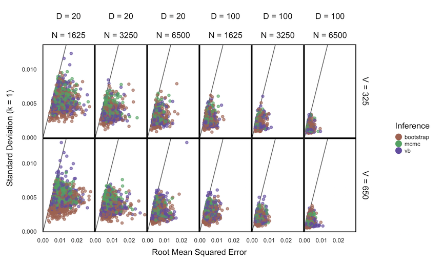
Figure 2: A summary of the errors and uncertainty across models and regimes for the $\beta_{vk}$ in Figure 1 and Supplementary Figure 10. On the $x$-axis, we plot the difference between posterior median and the true value, after having square-root transformed. On the $y$-axis, we provide the standard deviation of the posterior samples for each $v$, along the first dimension $K=1$. Columns are indexed as in Figure 1, but now rows provide different values of $V$.

The drift of points to the bottom left as $N$ and $D$ increase reflects the improved accuracy and concentration of all inference techniques when the number of samples and total count within samples increase. Note that few points lie above the identity standard deviation line – this suggests that the posteriors may be misleadingly narrow. Finally, we find that the scale of errors and concentration in the $V=325$ and $V=650$ cases are comparable. Considering that there is the same number of documents available for estimating each individual $\beta_{vk}$, this is not surprising.

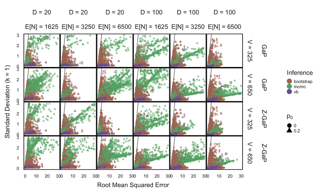
Figure 3: A version of Figure 2 for the NMF simulation experiment. The figures are read similarly, except there are a larger number of experimental configurations – rows now distinguish the assumed model and shapes represent the true value of $p_{0}$. Further, while the first row of column labels still gives $D$, the second row gives $\mathbb{E}\left[{N}\right]$ instead of $N$. Note that we also now truncate the $x$ and $y$ axes, and not all points are visible. For example, most MCMC samples in the last panel in the second row have errors and SDs larger than what is displayed, and so are missing.

For the NMF experiment, we use similar parameters, except now we introduce a zero-inflation probability, $p_{0}\in\{0,0.2\}$, and have control only over the expected total count per sample $\mathbb{E}\left[{N}\right]$, rather than $N$. When $p_{0}>0$, we perform inference when the true $p_{0}$ is provided and also when $p_{0}$ is (incorrectly) assumed to be zero. To modulate $\mathbb{E}\left[{N}\right]$, we vary $a_{0}$ and $b_{0}$ so that $\mathbb{E}\left[{N}\right]=\frac{b_{0}}{a_{0}}KV\in\{1625,3250,6500\}$, matching the LDA experiment. As before, we vary the number of samples $D\in\{20,100\}$ but fix the number of latent factors $K$ at 2. Figure 3 summarizes the estimation error across regimes, and is read in the same way as Figure 2, with two exceptions,

1. Instead of providing the fixed values of $N$, we display $\mathbb{E}\left[{N}\right]$.

2. We must distinguish between different $p_{0}$ regimes, and whether or not the inferential procedure assumed $p_{0}$ was 0 or was given the true $p_{0}$. The true value of $p_{0}$ is marked by the second row of column labels, and inference where $p_{0}$ was provided is denoted by the row label Z-GaP, while those rows marked GaP assumed $p_{0}=0$.

The associated posterior density display is given in Supplementary Figures 11 and 12.

The results in Figure 3 are more problematic than those in Figure 2. First, the standard errors are no longer comparable across methods, with those for the MCMC sampling procedure appearing much larger across many simulation configurations. Second, the error rates are substantially larger than those in LDA. Examining Supplementary Figures 11 and 12, it appears that lack of identifiability in the NMF model may be affecting our ability to evaluate the resulting fits. The only way to distinguish between models $\left(c\Theta\right)\left(\frac{1}{c}B\right)^{T}$ and $\Theta B^{T}$ is through the prior, and the prior may not be strong enough to guide inference to the right scaling.

Further, examining Supplementary Figure 11, we note many cases where estimation fails to converge or concentrates around the incorrect value, though this may be related to rescaling. Generally, we do not find a direct probabilistic-programming implementation of the GaP or Z-GaP models reliable in the regimes under consideration, even when $p_{0}$ is known.

Next we consider a simulation experiment involving the unigram model. We use the same configurations of $D$, $V$, and $N$ as in the LDA and NMF experiments above. The parameter controlling the rate of evolution on the simplex, $\sigma_{0}^{2}$, is set to 1 throughout. During inference, $\sigma_{0}^{2}$ is not assumed known, and is instead modeled as an $\text{InvGamma}\left(1,1\right)$ across all simulation settings.

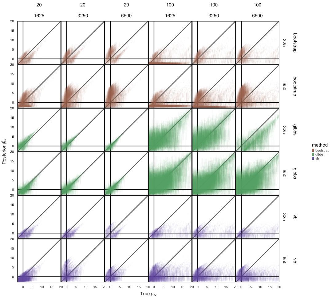
Figure 13: A comparison of the posterior $p\left(\mu_{tv}|x\right)$ to the known underlying $\mu_{tv}$, in the unigram simulation experiment. The $x$-axis for each interval corresponds to the true $\mu_{tv}$ for one species at one timepoint, while the vertical intervals cover the 25% to 75% quantiles of samples from the posterior $p\left(\mu_{tv}|x\right)$. Different panels distinguish between configurations of $D$, $N$, $V$, and posterior sampling schemes. Posteriors from MCMC sampling seem to correctly recover the true underlying $\mu_{tv}$, while discrepancies arise for both VB and the bootstrap.

In the NMF and LDA experiments, we could visualize fitted posteriors over $\theta_{i}$ and $\beta_{j}$ as two-dimensional smoothed scatterplots, since we set $K=2$. In contrast, this unigram experiment involves a $V$-dimensional parameter $\mu_{t}$ evolving over time – this precludes any direct analog to Figure 1 or Supplemental Figure 11. Instead, in Figure 13, we visualize the true $\mu_{tv}$ against posterior intervals for the one-dimensional $p\left(\mu_{tv}|x\right)$, across all configurations of simulation parameters.

Evidently, MCMC provides accurate posterior estimates, while VB and the bootstrap estimates deviate from the true $\mu_{tv}$. First, when the true $\mu_{tv}$ is small small, the posterior estimates from VB and the bootstrap are too large. This is not as much a reason for concern as it might appear at first, however, as the parameters $\mu_{t}$ are passed through a softmax before being mapped to probabilities. After this transformation, the difference between, say, $\mu_{tv}=10^{-2}$ and $\mu_{tv}=10^{-5}$ is relatively unimportant. Second, posterior estimates for $\mu_{tv}$ for large positive values of the parameter tend to be biased downards, to a degree that can’t be simply explained as an effect of the prior, as such a strong bias is not present among the MCMC-sampled posteriors.

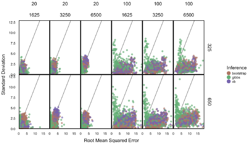
Figure 14: A simplification of Figure 13, displaying RMSE when using posterior medians to estimate simulation $\mu_{tv}$s ($x$-axis) and the standard deviations of posterior marginals ($y$-axis), across experimental configurations. Generally, MCMC sampled posteriors seem to be the most reliable, across simulation configurations.

To simplify the comparison between methods, we can also display the unigram analog of Figure 2 – this is given in Supplementary Figure 14. This display confirms our earlier observation, that posterior MCMC samples seem more reliable than either those from VB or the bootstrap, when using generic probabilistic programming for the Dynamic Unigram model, at least in problems with the dimensions we have considered.

4 Data Analysis

In applying probabilistic methods to microbiome data analysis, we concentrate on two questions,

1. Do these models fit the data well, and what techniques are available for performing this evaluation?

2. Supposing these models fit well, do they lend themselves to informative summaries of the original data?

To develop answers to these questions, we reanalyze the data of Dethlefsen and Relman (2011), a study of bacterial dynamics in response to antibiotic treatment. This study monitored the microbiomes of three patients over ten months, with two antibiotics time courses introduced in between, in order to study the effect of antibiotic perturbations within the context of natural long-term dynamics. By applying Principal Components Analysis, the study concluded that antibiotics cause substantial changes in short-term community composition, with certain species being substantially more resilient than others, and also detected long-term effects in one patient. The purpose of our case study is to compare these conclusions with those obtained through probabilistic latent variable models.

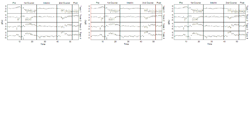
Figure 17: The analog of Figure 4 for Subject D.

Variation in bacterial signatures tends to be dominated by strong inter-subject effects (Eckburg and others, 2005), and with only three subjects, there is little reason for a model which clusters across subjects. Hence, we choose to study one individual at a time. In this section, we focus on Subject F, who had been reported to exhibit incomplete recovery of the pre-antibiotic treatment bacterial community. However, analogous figures for the other two subjects are available as Supplementary Figures 17 through 20. There are 2582 distinct species across these samples, and we perform no pre-filtering, though most species are present in very low numbers.

It is possible that future studies may consider a similar design, but involve many more subjects. In this case, it would be possible to do better than model each subject separately. The simplest way to share information across subjects would be to still have separate topics $\beta_{k}^{s}$ for each individual $s$, but to place a common prior across all $\left(\beta_{k}^{s}\right)_{k,s}$. This approach has the disadvantage that topics are not directly comparable across subjects. An alternative that mitigates this issue would be to share topics $\left(\beta_{k}\right)_{k}$ across all individuals, choosing $K$ to be larger than would be appropriate for any single subject. In this case, it would be expected that some $\theta_{ik}$ would be near zero for some topics for all samples within a subject – that subject may never have samples drawn from a particular topic. It is possible to directly incorporate this behavior, in which some but not all topics are shared across subjects, into the model form by considering a hierarchical Dirichlet prior, rather than a standard one (Wallach, 2006; Teh and others, 2005).

In this case study, we focus on LDA and the Dynamic Unigram model. A similar study using GaP and Z-GaP is omitted, in light of the difficulties in estimation during the simulation studies. Throughout, we apply VB, though considering the results of the simulation study, we exercise caution when interpreting estimated uncertainties. We set $K=4$, based on the heuristic that a larger $K$ would be less meaningful, since there are only 56 timepoints. In cases where it is of interest to choose $K$ automatically, it would be possible to evaluate the likelihood of fitted models on a hold-out set, for a range of values of $K$, by fixing $\left(\hat{\beta}_{k}\right)_{k=1}^{K}$ and estimating new $\hat{\theta}_{i}$ for the hold-out samples (Blei and others, 2003). Indeed, this process reflects an advantage of probabilistic modeling: the Bayesian Occam’s razor ensures that the posterior probability of a model won’t always go up as $K$ increases – contrast this with ordinary $K$-means, where tailored methods like the Gap or Silhouette statistics must be studied (Rasmussen and Ghahramani, 2001; Tibshirani and others, 2001; Kaufman and Rousseeuw, 2009). Alternatively, the proposals of (Wallach and others, 2009) could be carried out. However, in this study, we guide the choice of $K$ based on what we find most useful for scientific interpretation, rather than that which necessarily gives the best fit over the entire population.

Note that we plot the fitted probabilities on a logit scale – for a raw vector of probabilities $\mathbf{p}=\left(p_{1},\dots,p_{D}\right)\in\mathcal{S}^{D-1}$, we plot $g\left(\mathbf{p}\right):=\left(\log p_{1}-\overline{\log\mathbf{p}},\dots,\log p_{K}-\overline{\log\mathbf{p}}\right)$, which are similar to log-odds, but centered according to the average log probability, rather than any reference class.

Both LDA and the Dynamic Unigram model are more computationally intensive than more common approaches, like principal components analysis (PCA) or multidimensional scaling (MDS), but are still amenable to routine application. For example, in the case studies below, LDA and the Dynamic Unigram model can both be compiled and run on a standard laptop in 5.62 and 30.0 minutes, respectively – the longer runtime of the Dynamic Unigram model is due to its larger number of parameters. Further, both approaches can be scaled to much larger datasets without requiring substantially more memory (but requiring somewhat longer training time) by applying stochastic variational inference (Hoffman and others, 2013; Kucukelbir and others, 2015).

4.1 Latent Dirichlet Allocation

The fitted parameter values are summarized in Figures 4 and 5. In Figure 4, rows represent topics, the $x$-axis represents time, and the $y$-axis gives the boxplots of posterior quantiles for each $\theta_{dk}$.

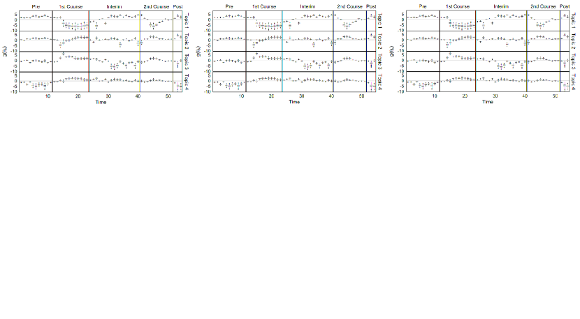
Figure 4: Boxplots represent approximate posteriors for estimated mixture memberships $\theta_{d}$, and their evolution over time. That is, each row of panels provides a different sequence of $\theta_{dk}$ for a single $k$, and different columns distinguish different phases of sampling. Note that the $y$-axis is on the $g$-scale, which is defined as a translated logit, $g\left(\mathbf{p}\right):=\left(\log p_{1}-\overline{\log\mathbf{p}},\dots,\log p_{K}-\overline{\log\mathbf{p}}\right)$. Note that the first and second antibiotic time courses result in meaningful shifts in these sequences, and that there appear to be long-term effects of treatment among bacteria in Topic 3.

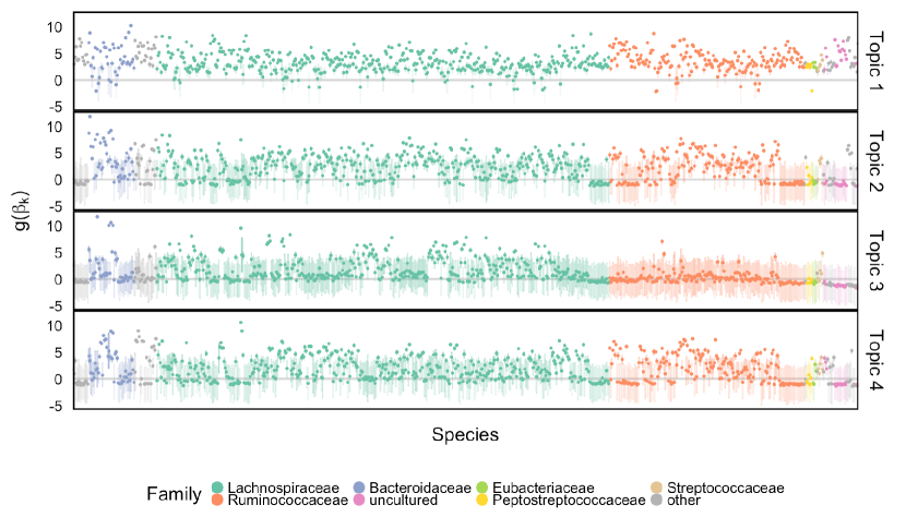
Figure 5: Each credible interval describes an approximate posterior for one $\beta_{vk}$. Coupled with Figure 4, this guides the interpretation of which bacterial taxa are more or less prevalent during antibiotic treatments. Each row of panels corresponds to one of the four topics, the $x$-axis indexes species, sorted according to phylogenetic relatedness, and the $y$-axis give transformed values of the species probability under that topic. Only the 750 most abundant species are shown. Note the disappearance of otherwise abundant species within Topics 2, 4, and to some extent, 1.

This figure draws attention to the two antibiotic time courses, which took place between days 12-23 and 41-51. Topic 1 seems to become prominent during the interim period between the two time courses, suggesting that this is the bacterial community that fills in the niches left empty during the first time course. Conversely, Topic 3 seems to represent those bacteria that were present initially but are eliminated during the first time course, though there is a hint of a recovery at the end of sampling. This topic seems most closely related to the finding reported in Dethlefsen and Relman (2011) that Subject F experienced long-term antibiotic effects on bacterial community composition. Topics 2 and 4 seem to be overrepresented during the antibiotic treatments. Topic 2 is elevated immediately after the antibiotic treatment. Topic 4 seems to summarize those bacteria that are initially negatively impacted by the antibiotic treatments, but which recover relatively quickly and have higher abundance at the end of the trial than at the beginning. The fact that Topics 2 and 4 are learned from the data without enforcing any temporal evolution structure on the samples suggests that under an antibiotic perturbation, the system exhibits differential recovery.

To interpret these topics in terms of their bacterial community fingerprint, we study the estimated topic distributions $\beta_{k}$. This is displayed in Figure 5. The four rows correspond to the $K=4$ estimated topics. Within a row, we show 95% credible intervals associated with the posterior samples for each bacterium. Different colors identify different taxonomic families, and bacteria are sorted according to evolutionary relatedness. For clarity, we have displayed only the 750 most abundant bacteria.

Considering the mixture probabilities in Figure 4, those bacteria with large probabilities in the second and fourth rows of Figure 5 constitute a large fraction of the samples taken during antibiotics time courses, reflecting those whose abundances increase rapidly (Topic 2) or are initially drop but then increase gradually (Topic 4) during the antibiotics time courses. These distributions are relatively more concentrated on a small subset of bacteria with high probabilities, reflected by the drop in logitted probabilities far below zero. This corresponds to a decrease in community diversity during antibiotic time courses. We also note groups of neighboring bacteria with similarly elevated topic probabilities. It is encouraging that, even without specifying smoothness along the phylogenetic tree in the prior for the $\beta_{k}$s, such smoothness emerges in the fitted model.

One disadvantage of plotting the posteriors for the $\beta_{k}$ in this way is that it is difficult to determine the identify of any particular bacterial species associated with a specific credible interval. It also hides any interesting variation that may be occurring among species not among the 750 most abundant. To address these issues, we have designed an interactive version, available online at https://statweb.stanford.edu/~kriss1/microbiome_plvm/vis.html. Alternatively, individual species that are primarily assigned to individual topics can be used to characterize the topics. For example, in Figure 6 we have screened all species for those that seem primarily associated with a single topic, and plotted them along with the topic for they are representative. Specifically, representatives of the $k^{th}$ topic were found by choosing the 50 species $v$ with the largest values of $\beta_{kv}-\sum_{k^{\prime}\neq k}\beta_{k^{\prime}v}$.

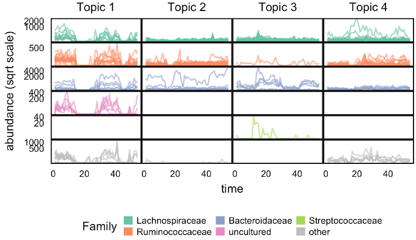
Figure 6: Individual species that have been identified as prototypical of single topics are highlighted here, to provide a characterization of topics linked to the original bacterial abundance data. Rows and columns of panels correspond to taxonomic families and estimated topics, respectively, and each trajectory gives the abundance of a single species over time. Note that the $y$-axis is on a square root scale. This view provides more evidence for the interpretation of the four topics as (1) decreased abundance during antibiotic time courses (2) increased abundance during antibiotic time courses (3) disappearance after first time course, and (4) delayed but sustained increase after first time course.

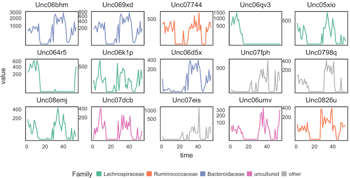
Figure 21: Rather than displaying all representative species together, as in Figure 6, we can sort species according to how representative they are of an individual topic. Here, the 15 species most strongly associated with Topic 1 are given. The panels are to be read from left to right and from top to bottom, to go in decreasing value of association. Note that the $y$-axis is on a square root scale.

This allows an interpretation of the topics in terms of the raw data, and the display reinforces the findings of Figures 4 and 5. In particular, this view makes clear how much variation there is in species abundances within taxonomic families – compare Topics 1 and 2 among representative Lachnospiraceae and Bacteroides, for example. Instead of displaying all species together, Supplementary Figures 21 through 24 sort individual species by the topic representativeness measure.

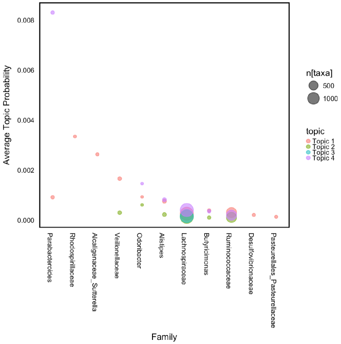
Figure 25: We can search for entire taxonomic families that seem associated with individual topics. Here we calculate the average of the topic representativeness statistic $\beta_{kv}-\sum_{k^{\prime}\neq k}\beta_{k^{\prime}v}$ across all species $v$ within each Family. Only those families that are most associated with a topic are displayed here. The sizes of circles represents the number of species within the family, which can be used to gauge the variability of the estimate. Compare this view with Supplementary Figure 26.

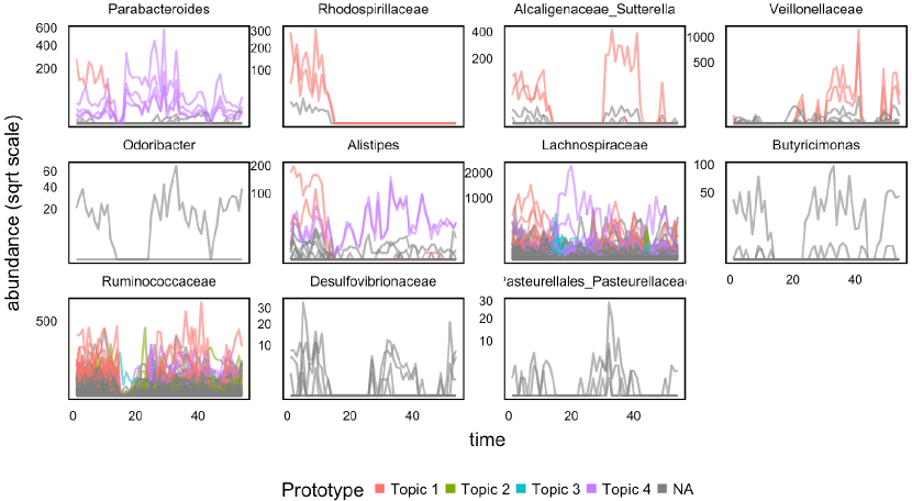
Figure 26: All species within the families screened out from Figure 25 are displayed here. Species among the representatives displayed in Figure 6 are colored according to the topics of they are prototypical. Grey series still contribute to the average family-topic association measure, but were not among the 50 prototypes for each topic. This view suggests that the Rhodospillaceae, Alcaligenaceae and Parabacteroides may have a large fractions of representatives from Topics 3, 1, and 2, respectively. Note that as before, abundances are plotted on a square root scale.

Similar approaches can be employed to identify taxa that disproportionately contain species with high membership in particular topics. For example, we can compute the average topic representativeness statistic defined above across all species within a taxonomic family in order to characterize that family. Families that are highly associated with individual topics are displayed in Supplementary Figures 25 and 26.

4.2 Dynamic Unigram model

While we can interpret the LDA-estimated $\hat{\theta}_{d}$ according to their temporal context, this information was never directly provided to the algorithm. In contrast, we can apply the Dynamic Unigram model to the same data, which explicitly models temporal evolution. Unlike LDA, however, this model does not seek latent mixture structure. Our primary results are displayed in Figure 7.

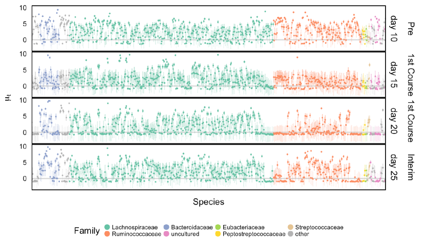
Figure 7: Each posterior credible interval refers to one $\mu_{vt}$. The rows are a subset of times $t$ around the first antibiotic time course. The first row corresponds to a timepoint from before the treatment, the middle two from during the antibiotics time course, and the bottom from after the time course was stopped. Otherwise, this display is read in the same way as Figure 5. This view provides one way of smoothing abundance time series, to see how different species respond to antibiotic treatment.

Each row in this figure is interpreted similarly to a row in Figure 5, except now they correspond to estimated proportions over time $g\left(\mu_{t}\right)$ rather than transformed topics $g\left(\beta_{k}\right)$. Only four of the 54 total timepoints is displayed, highlighting a time window around the first antibiotic time course. Such a display implicitly assumes a relatively smooth interpolation between timepoints, which is enforced by the form of the Dynamic Unigram model.

This analysis yields conclusions similar to those obtained through LDA, though reaching them requires somewhat more effort. For example, on day 10, most $g\left(\mu_{tv}\right)$’s have most of their mass concentrated above zero, and not many are positioned exceptionally far form the bulk. This is consistent with higher community diversity before the antibiotic time course. On the other hand, at time 15, one day after the time course began, most species have quantiles lower than zero, while a few are positioned much higher than the rest. This corresponds to a less diverse community, whose membership is concentrated on those species with outlying intervals. This decrease in diversity seems most profound at time 20; by time 25, during the interim, much of the community seems to have recovered.

Further, while we continue to see differential recovery across bacteria, the effect is not as obvious as in LDA, where this effect was decomposed across topics. For example, many subintervals of Lachnospiraceae seem to return to their pre-antibiotics levels by time 25, while the Ruminococceae continue to have low values of $\mu_{tv}$.

4.3 Posterior Predictive Checks

While we have found both LDA and the Dynamic Unigram model qualitatively useful, it is still important to seek more formal diagnostics of model fit. Here, we consider several posterior predictive checks, as explained in Section 2.5.

To this end, in Figure 8, we plot observed time series for a random subset of the 350 most abundant bacteria and contrast them with samples from the posterior predictive according to the four topic LDA model of Section 4.1 and the unigram model of Section 4.2. Each subpanel corresponds to a single species. The black lines represent observed time series. Note that the $y$-axis scales vary, as some species are much more abundant than others. Each dot is a simulated timepoint from a posterior predictive time series. Formally, this corresponds to the choice $T\left(x\right)=\left(x_{\cdot v}\right)_{v\in\mathcal{V}}$ where the random subset $\mathcal{V}$ indexes the displayed species.

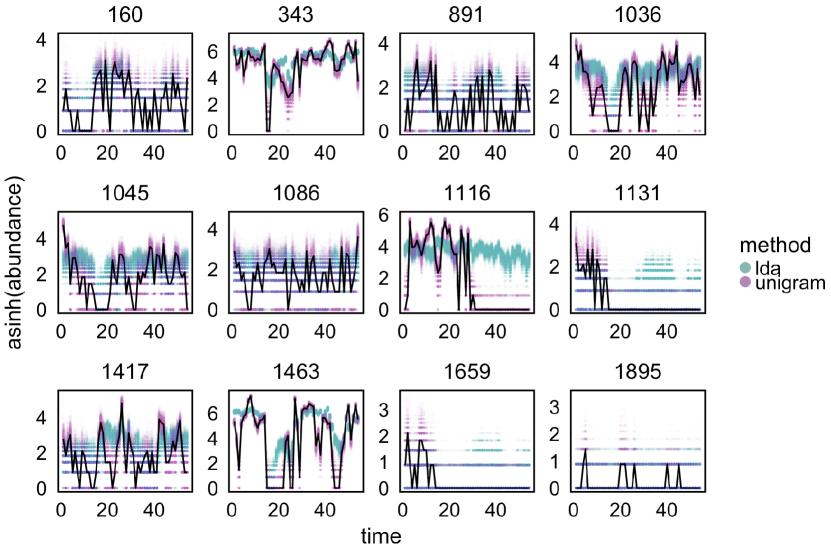
Figure 8: We can visualize the simulated time series for a subset of species and compare them with the observed ones, as a posterior check. Each panel represents one species. The black lines represent the observed $\mathop{\mathrm{missing}}{asinh}$-transformed abundances for subject F over time. The blue and purple dots give the posterior predictive realizations for these species over time, according to LDA and the Dynamic Unigram model, respectively.

For LDA, the posterior predictive time series are on the appropriate scale with approximately the correct shape. However, we observe two substantial types of departures between simulated and observed data. First, for series with larger counts, the posterior predictive tends to oversmooth. For example, the drop to 0 in species 343 is not captured in any posterior predictive samples. Similar oversmoothing is visible in species 1036, 1116, and 1463. A more startling type of departure occurs in the second half of series 1116. Here, the posterior predictive distribution places most mass on the event that the bacterial time series rebounds to its initial abundance when in reality the species vanishes during the second antibiotic time course, never to return. A potential explanation for LDA’s failure to capture this pattern is that few highly abundant species disappear after the second time course, and hence they are not captured by the global LDA summary. This suggests a technique for highlighting outlier species: we can look at the average discrepancy between observed series and their posterior predictive samples.

On the other hand, for the Dynamic Unigram model, the posterior predictive distribution places most of its support close to the observed species series. Usually, this is desirable behavior, indicating good model fit. However, here, there is reason for concern – the unigram model may not do much more than fit empirical proportions at each timepoint, and there may be potential to produce more succinct summaries that still preserve the essential structure of the data. That is, the unigram model seems over-parameterized, simply memorizing the input.

An alternative posterior predictive check compares PCA scores and loadings in the true and posterior predictive data. Our motivation is that many microbiome studies base their findings on views generated by PCA, so it would be encouraging if our probabilistic summaries typically agree with the reductions produced by PCA. Formally, we construct $T\left(x\right)=\left(u_{1},u_{2},\lambda_{1},\lambda_{2},v_{1},v_{2}\right)$ where $\left(u_{i}\right)$, $\left(\lambda_{i}\right)$ and $\left(v_{j}\right)$ are left singular vectors, eigenvalues, and right singular vectors of $x$, respectively.

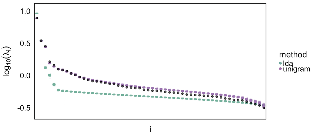
Figure 9: As a posterior predictive check, we compute eigenvalues of data simulated from the fitted LDA model. The clouds of points summarize the posterior predictive distribution, while the black circles represent observed data eigenvalues. Note that the $y$-axis are logged eigenvalues. Evidently, the four-topic model effectively creates a rank-four approximation of the original data.

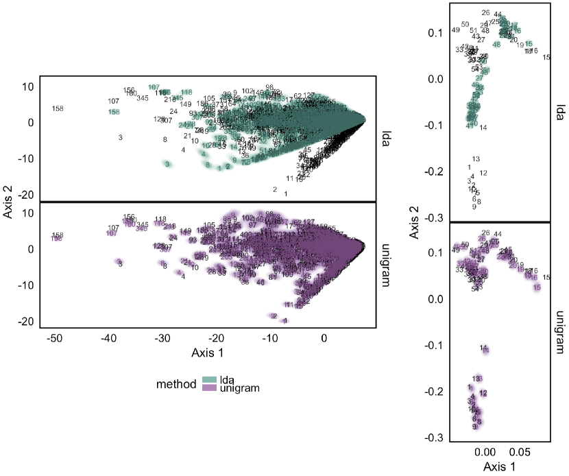
Figure 16: The eigenvalues displayed in Figure 9 correspond to PCA results computed on posterior predictive samples, which are aligned and overlaid here. The left pair of panels give scores for each species, while the right pair provide loadings for each timepoint. The individual posterior samples have been smoothed into contours, while the posterior medians are displayed as shaded text. The observed data PCA results, after alignment with posterior samples, are displayed as black text.

Figure 9 gives the PCA eigenvalues between the true and posterior predictive samples, after applying an $\mathop{\mathrm{missing}}{asinh}$-transformation and filtering to the 1000 highest-variance bacteria. The associated scores and loadings figures are available as Supplementary Figure 16. In Figure 9, each black point provides the log-eigenvalue observed in the original data. The blue and purple clouds consistent of small, semi-transparent, horizontally-jittered points associated with eigenvalues from posterior predictive samples generated by LDA and the Dynamic Unigram model, respectively. For LDA, the posterior predictive samples have comparable top four eigenvalues, but rapidly drop-off between the fourth and fifth eigenvalues. On the other hand, the observed data have a more steady decline. This is likely a consequence of using $K=4$ topics in the LDA model, which would be consistent with the matrix factorization view of LDA described in Section 2.4. Considering these scree plots, it may be safe to increase $K$ in follow-up analysis, as long as topics remain interpretable. In contrast, the eigenvalues for the Dynamic Unigram model closely match those in the observed data – even overestimating the size of small eigenvalues – lending further evidence to the claim that this model is over-parameterized.

4.4 Comparison with principal coordinates

There is value in comparing this text-modeling based approach to the data from (Dethlefsen and Relman, 2011) with the analysis carried out in the original publication, based on principal coordinates analysis (PCoA) using a UniFrac distance. Both approaches accentuate the dramatic change in microbiome composition immediately following the administration of antibiotics, and both suggest the overall resilience of the microbiome, in the sense that the community returns to the preantibiotic state after several days. Further, both distinguish subject F as only making an incomplete recovery after the first antibiotic treatment.

On the other hand, some findings are more easily accessible when using the probabilistic approach. For example, the availability of topics with mixed memberships strikes a balance between the continuous gradient representation of principal coordinate analysis of (Dethlefsen and Relman, 2011) and the discrete clusters provided by standard clustering techniques, which appear elsewhere in the microbiome literature (DiGiulio and others, 2015; McMurdie and Holmes, 2014). This simplifies the taxonomic characterization of different communities – with principal coordinates, it would be necessary to find species correlated with the principal coordinate axes, and indeed no visual representations of taxa ever appear in the figures of Dethlefsen and Relman (2011). Similarly, by studying individual topics, we find there is more variation within taxonomic families than is ever discussed in the original refernece. Further, through posterior predictive checks, we can perform model assessment in a way that is not so straightforwards with PCoA, and more broadly speaking, we by adopting probabilistic methods, we are able to describe the uncertainty associated with mixed membership and topic estimate.

That said, PCoA enjoys certain advantages over the probabilistic approaches that have been the focus of this work. Perhaps most importantly, PCoA can be run in seconds, which makes it much more useful for interactive analysis. Second, by using the UniFrac distance, PCoA is able to account for the phylogenetic relatedness between taxa, encouraging phylogenetically similar taxa to play similar roles in the resulting ordination. Finally, the visual representation of samples provided by PCoA – simply a two-dimensional scatter of the samples – is more easily digestible than the simultaneous display of all parameters in probability models.

Broadly speaking, it seems valuable to have both types of tools available for practical scientific work. Ordination techniques like PCoA are useful for describing the relationship between sets of samples, in a way that requires little effort in either estimation or display. However, for more richly structured summaries, which are amenable to uncertainty quantification and model evaluation, probabilistic methods are ideal. We imagine a workflow in which researchers quickly develop a sense of their data using ordination, and then refine and critique their analysis using latent variables models.

5 Discussion

We have described the utility of taking a probabilistic modeling perspective in the analysis of microbiome data. We have provided a detailed implementation of benchmark analysis approaches, along with exploratory visualization of fitted parameters and model assessment through posterior predictive checks. Through simulation, we have established heuristics for determining the appropriateness of applying different models and inference mechanisms, depending on the overall data generation regime. On a real microbiome data analysis problem, we have characterized the advantages and limitations of two probabilistic modeling techniques. Rather than focusing on any single model, like most earlier work, we have emphasized the practice of contrasting, critiquing, and learning from multiple alternatives. Throughout, we have emphasized both insights, in terms of estimated parameters, as well as uncertainty, in the form of full approximate posterior distributions. We hope our efforts help to widen the biostatistician’s toolbox and clarify the practical advantages and limitations of different approaches to microbiome data.

Microbiome studies are a source of richly structured, high-dimensional data, coupled with novel scientific problem setups. For example, in the antibiotics data set described here, we have already encountered structure in the form of zero-inflated counts, time series with changepoints, and apriori known phylogenetic relationships between features. It is anticipated that future microbiome studies will collect an increasing number of samples as well as more data sources per sample – spectral and genomic, in addition bacterial abundance, for example (Jansson and Baker, 2016). Further, the investigations often revolve around a combination of ecological community characterization and medically-relevant identification of treatment effects. We believe we have only begun to see the potential for probabilistic methods to guide careful scientific reasoning – which emphasizes both insights and the degree of uncertainty about them – in these complex scenarios.

6 Supplementary Material

Supplementary material is available online at http://biostatistics.oxfordjournals.org.

7 Reproducibility

Code for all simulations, data analysis, and figures is available at https://github.com/microbiome\_plvm. Detailed instructions are available in the repository README.md. Further, a docker image with all software requirements preinstalled is available from https://hub.docker.com/r/krisrs1128/microbiome_plvm/, and the corresponding Dockerfile is provided in the github repository.

8 Supplementary Figures

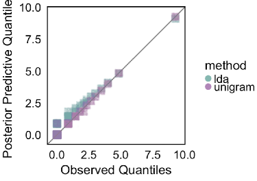
Figure 15: As a posterior check, we compare the observed with simulated data quantiles, using a qq-plot. To reduce overlap, we have introduced a uniform $\left[0,0.2\right]$ jitter on both axes. Further, the points are semi-transparent – this makes it easy to see that most quantiles map to 0, which is expected, considering the sparsity of the data. From this view, we see that the LDA model tends to underestimate the overall number of zeros in the data, while the Dynamic Unigram model matches the observed quantiles almost exactly.

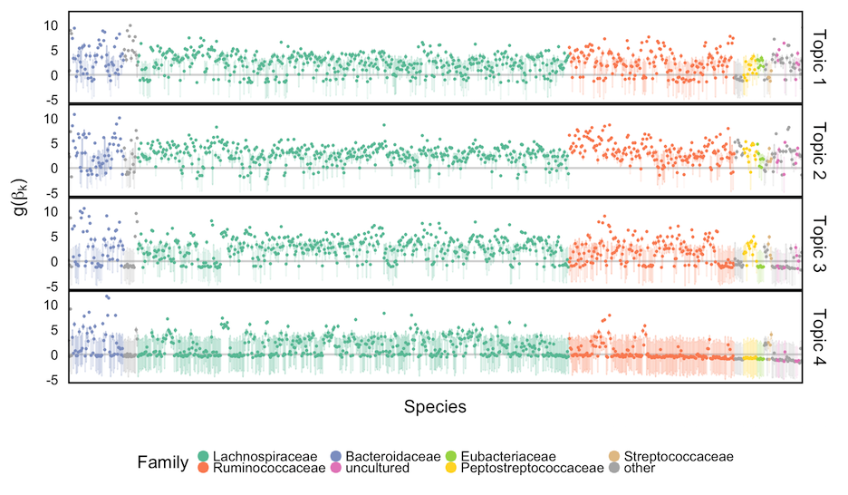
Figure 18: The analog of Figure 5 for Subject D.

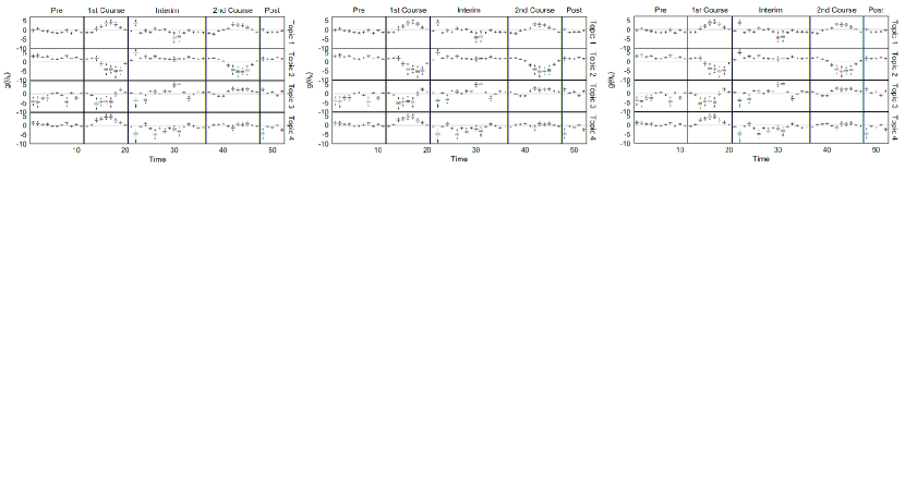
Figure 19: The analog of Figure 4 for Subject E.

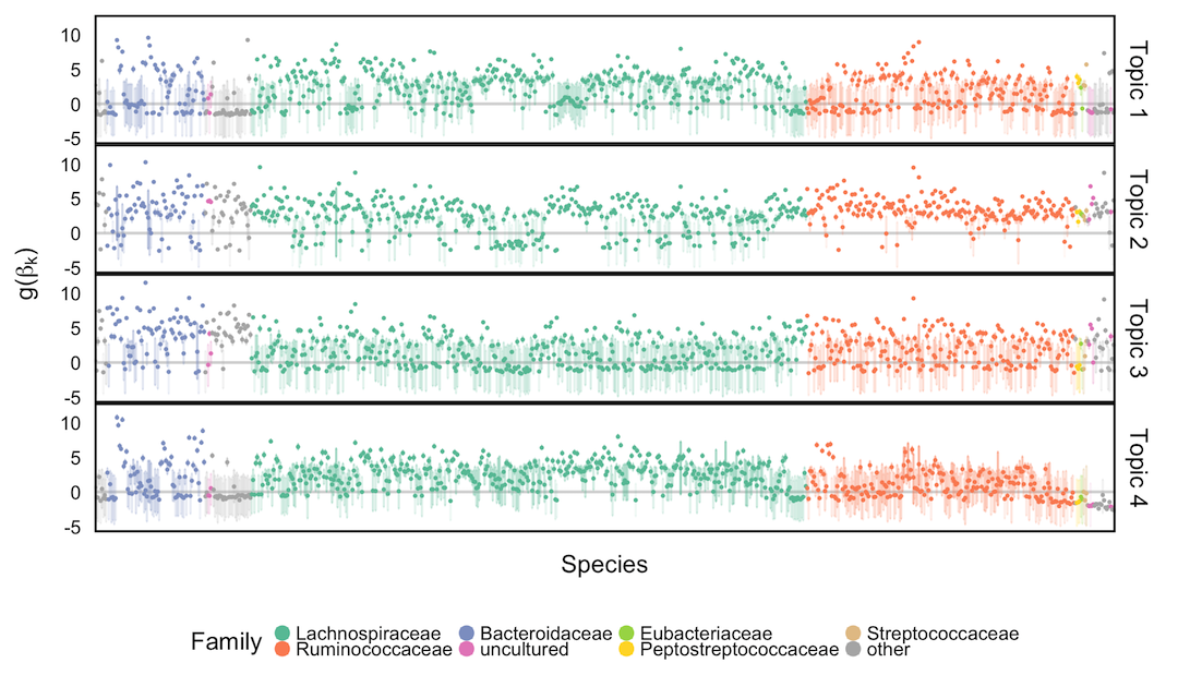
Figure 20: The analog of Figure 5 for Subject E.

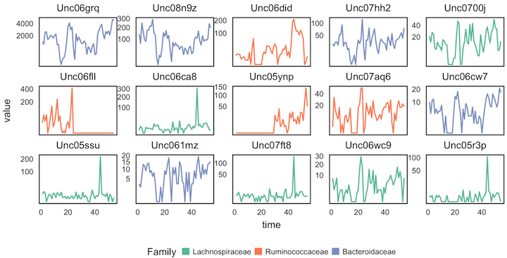
Figure 22: The analog of Figure 21 for Topic 2..

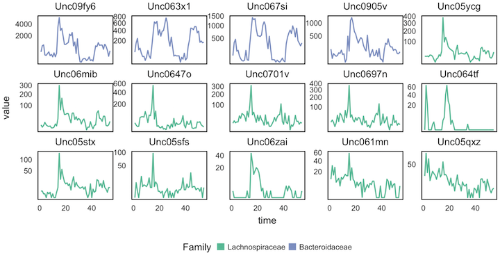
Figure 23: The analog of Figure 21 for Topic 3.

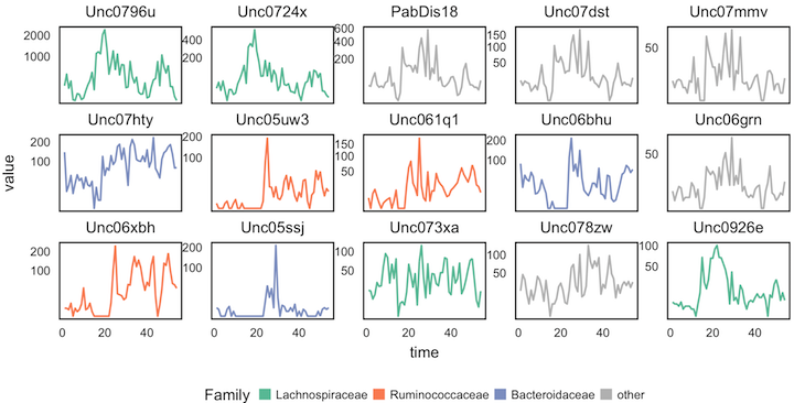
Figure 24: The analog of Figure 21 for Topic 4.

References

- Berry and others (2007) Berry, Michael W, Browne, Murray, Langville, Amy N, Pauca, V Paul and Plemmons, Robert J. (2007). Algorithms and applications for approximate nonnegative matrix factorization. Computational statistics & data analysis 52(1), 155–173.
- Blei and Lafferty (2006) Blei, David M and Lafferty, John D. (2006). Dynamic topic models. In: Proceedings of the 23rd international conference on Machine learning. ACM. pp. 113–120.
- Blei and others (2003) Blei, David M, Ng, Andrew Y and Jordan, Michael I. (2003). Latent dirichlet allocation. Journal of machine Learning research 3(Jan), 993–1022.
- Callahan and others (2017) Callahan, Benjamin J, McMurdie, Paul J and Holmes, Susan P. (2017, jul). Exact sequence variants should replace operational taxonomic units in marker-gene data analysis. The ISME Journal.
- Canny (2004) Canny, John. (2004). Gap: a factor model for discrete data. In: Proceedings of the 27th annual international ACM SIGIR conference on Research and development in information retrieval. ACM. pp. 122–129.
- Carpenter and others (2016) Carpenter, Bob, Gelman, Andrew, Hoffman, Matt, Lee, Daniel, Goodrich, Ben, Betancourt, Michael, Brubaker, Michael A, Guo, Jiqiang, Li, Peter and Riddell, Allen. (2016). Stan: A probabilistic programming language. Journal of Statistical Software 20.
- Chen and others (2013) Chen, Jun, Bushman, Frederic D, Lewis, James D, Wu, Gary D and Li, Hongzhe. (2013). Structure-constrained sparse canonical correlation analysis with an application to microbiome data analysis. Biostatistics 14(2), 244–258.
- Chen and Li (2013) Chen, Jun and Li, Hongzhe. (2013). Variable selection for sparse dirichlet-multinomial regression with an application to microbiome data analysis. The annals of applied statistics 7(1).
- Chen and others (2012) Chen, Xin, He, TingTing, Hu, Xiaohua, Zhou, Yanhong, An, Yuan and Wu, Xindong. (2012). Estimating functional groups in human gut microbiome with probabilistic topic models. IEEE transactions on nanobioscience 11(3), 203–215.
- Dethlefsen and Relman (2011) Dethlefsen, Les and Relman, David A. (2011). Incomplete recovery and individualized responses of the human distal gut microbiota to repeated antibiotic perturbation. Proceedings of the National Academy of Sciences 108(Supplement 1), 4554–4561.
- DiGiulio and others (2015) DiGiulio, Daniel B, Callahan, Benjamin J, McMurdie, Paul J, Costello, Elizabeth K, Lyell, Deirdre J, Robaczewska, Anna, Sun, Christine L, Goltsman, Daniela SA, Wong, Ronald J, Shaw, Gary and others. (2015). Temporal and spatial variation of the human microbiota during pregnancy. Proceedings of the National Academy of Sciences 112(35), 11060–11065.
- Eckburg and others (2005) Eckburg, Paul B, Bik, Elisabeth M, Bernstein, Charles N, Purdom, Elizabeth, Dethlefsen, Les, Sargent, Michael, Gill, Steven R, Nelson, Karen E and Relman, David A. (2005). Diversity of the human intestinal microbial flora. science 308(5728), 1635–1638.
- Fukuyama (2017) Fukuyama, Julia. (2017). Adaptive gpca: A method for structured dimensionality reduction. arXiv preprint arXiv:1702.00501.
- Fukuyama and others (2017) Fukuyama, Julia, Rumker, Laurie, Sankaran, Kris, Jeganathan, Pratheepa, Dethlefsen, Les, Relman, David A and Holmes, Susan P. (2017). Multidomain analyses of a longitudinal human microbiome intestinal cleanout perturbation experiment. PLoS Computational Biology 13(8), e1005706.
- Gelman and Shalizi (2013) Gelman, Andrew and Shalizi, Cosma Rohilla. (2013). Philosophy and the practice of bayesian statistics. British Journal of Mathematical and Statistical Psychology 66(1), 8–38.
- Gilbert and others (2014) Gilbert, Jack A, Jansson, Janet K and Knight, Rob. (2014). The earth microbiome project: successes and aspirations. BMC biology 12(1), 69.
- Griffiths and Steyvers (2004) Griffiths, Thomas L and Steyvers, Mark. (2004). Finding scientific topics. Proceedings of the National academy of Sciences 101(suppl 1), 5228–5235.
- Hoffman and others (2013) Hoffman, Matthew D, Blei, David M, Wang, Chong and Paisley, John William. (2013). Stochastic variational inference. Journal of Machine Learning Research 14(1), 1303–1347.
- Holmes and others (2012) Holmes, Ian, Harris, Keith and Quince, Christopher. (2012). Dirichlet multinomial mixtures: generative models for microbial metagenomics. PloS one 7(2), e30126.
- Human Microbiome Project Consortium (2012) Human Microbiome Project Consortium. (2012). Structure, function and diversity of the healthy human microbiome. Nature 486(7402), 207–214.
- Jansson and Baker (2016) Jansson, Janet K and Baker, Erin S. (2016). A multi-omic future for microbiome studies. Nature microbiology 1, 16049.
- Jiang and others (2017) Jiang, Xingpeng, Hu, Xiaohua and Xu, Weiwei. (2017). Microbiome data representation by joint nonnegative matrix factorization with laplacian regularization. IEEE/ACM Transactions on Computational Biology and Bioinformatics 14(2), 353–359.
- Kaufman and Rousseeuw (2009) Kaufman, Leonard and Rousseeuw, Peter J. (2009). Finding groups in data: an introduction to cluster analysis, Volume 344. John Wiley & Sons.
- Krestel and others (2009) Krestel, Ralf, Fankhauser, Peter and Nejdl, Wolfgang. (2009). Latent dirichlet allocation for tag recommendation. In: Proceedings of the third ACM conference on Recommender systems. ACM. pp. 61–68.
- Kucukelbir and others (2015) Kucukelbir, Alp, Ranganath, Rajesh, Gelman, Andrew and Blei, David. (2015). Automatic variational inference in stan. In: Advances in neural information processing systems. pp. 568–576.
- Lee and Seung (2001) Lee, Daniel D and Seung, H Sebastian. (2001). Algorithms for non-negative matrix factorization. In: Advances in neural information processing systems. pp. 556–562.
- Love and others (2014) Love, Michael I, Huber, Wolfgang and Anders, Simon. (2014). Moderated estimation of fold change and dispersion for rna-seq data with deseq2. Genome biology 15(12), 550.
- McMurdie and Holmes (2014) McMurdie, Paul J and Holmes, Susan. (2014). Waste not, want not: why rarefying microbiome data is inadmissible. PLoS Comput Biol 10(4), e1003531.
- Nigam and others (2000) Nigam, Kamal, McCallum, Andrew Kachites, Thrun, Sebastian and Mitchell, Tom. (2000). Text classification from labeled and unlabeled documents using em. Machine learning 39(2), 103–134.
- Rasmussen and Ghahramani (2001) Rasmussen, Carl Edward and Ghahramani, Zoubin. (2001). Occam’s razor. In: Advances in neural information processing systems. pp. 294–300.
- Romero and others (2014) Romero, Roberto, Hassan, Sonia S, Gajer, Pawel, Tarca, Adi L, Fadrosh, Douglas W, Nikita, Lorraine, Galuppi, Marisa, Lamont, Ronald F, Chaemsaithong, Piya, Miranda, Jezid and others. (2014). The composition and stability of the vaginal microbiota of normal pregnant women is different from that of non-pregnant women. Microbiome 2(1), 4.
- Rubin and others (1984) Rubin, Donald B and others. (1984). Bayesianly justifiable and relevant frequency calculations for the applied statistician. The Annals of Statistics 12(4), 1151–1172.
- Schloss and Handelsman (2007) Schloss, Patrick D and Handelsman, Jo. (2007). The last word: books as a statistical metaphor for microbial communities. Annu. Rev. Microbiol. 61, 23–34.
- Segata and others (2011) Segata, Nicola, Izard, Jacques, Waldron, Levi, Gevers, Dirk, Miropolsky, Larisa, Garrett, Wendy S and Huttenhower, Curtis. (2011). Metagenomic biomarker discovery and explanation. Genome biology 12(6), R60.
- Shafiei and others (2015) Shafiei, Mahdi, Dunn, Katherine A, Boon, Eva, MacDonald, Shelley M, Walsh, David A, Gu, Hong and Bielawski, Joseph P. (2015). Biomico: a supervised bayesian model for inference of microbial community structure. Microbiome 3(1), 8.
- Teh and others (2004) Teh, Yee Whye, Jordan, Michael I, Beal, Matthew J and Blei, David M. (2004). Sharing clusters among related groups: Hierarchical dirichlet processes. In: NIPS. pp. 1385–1392.
- Teh and others (2005) Teh, Yee W, Jordan, Michael I, Beal, Matthew J and Blei, David M. (2005). Sharing clusters among related groups: Hierarchical dirichlet processes. In: Advances in neural information processing systems. pp. 1385–1392.
- Tibshirani and others (2001) Tibshirani, Robert, Walther, Guenther and Hastie, Trevor. (2001). Estimating the number of clusters in a data set via the gap statistic. Journal of the Royal Statistical Society: Series B (Statistical Methodology) 63(2), 411–423.
- Wallach (2006) Wallach, Hanna M. (2006). Topic modeling: beyond bag-of-words. In: Proceedings of the 23rd international conference on Machine learning. ACM. pp. 977–984.
- Wallach and others (2009) Wallach, Hanna M, Murray, Iain, Salakhutdinov, Ruslan and Mimno, David. (2009). Evaluation methods for topic models. In: Proceedings of the 26th annual international conference on machine learning. ACM. pp. 1105–1112.
- Wang and Titterington (2005) Wang, Bo and Titterington, DM. (2005). Inadequacy of interval estimates corresponding to variational bayesian approximations. In: AISTATS.
- Wang and Zhang (2013) Wang, Yu-Xiong and Zhang, Yu-Jin. (2013). Nonnegative matrix factorization: A comprehensive review. IEEE Transactions on Knowledge and Data Engineering 25(6), 1336–1353.
- Zhou and Carin (2015) Zhou, Mingyuan and Carin, Lawrence. (2015). Negative binomial process count and mixture modeling. IEEE Transactions on Pattern Analysis and Machine Intelligence 37(2), 307–320.