Fast Bayesian inference of the multivariate Ornstein-Uhlenbeck process

Abstract

The multivariate Ornstein-Uhlenbeck process is used in many branches of science and engineering to describe the regression of a system to its stationary mean. Here we present an $O(N)$ Bayesian method to estimate the drift and diffusion matrices of the process from $N$ discrete observations of a sample path. We use exact likelihoods, expressed in terms of four sufficient statistic matrices, to derive explicit maximum a posteriori parameter estimates and their standard errors. We apply the method to the Brownian harmonic oscillator, a bivariate Ornstein-Uhlenbeck process, to jointly estimate its mass, damping, and stiffness and to provide Bayesian estimates of the correlation functions and power spectral densities. We present a Bayesian model comparison procedure, embodying Ockham’s razor, to guide a data-driven choice between the Kramers and Smoluchowski limits of the oscillator. These provide novel methods of analyzing the inertial motion of colloidal particles in optical traps.

DOI: 10.1103/PhysRevE.98.012136

I Introduction

The multivariate Ornstein-Uhlenbeck process is widely used in many branches of science and engineering to describe the regression of a system to its stationary mean. Its importance arises from the fact that it is the only continuous stochastic process that is simultaneously stationary, Gaussian and Markovian doob1942brownian ; doob1953stochastic . Therefore, the process is fully characterized by its stationary and conditional distributions, each of which is a multivariate Gaussian, with mean and variance determined by the regression rates and diffusion coefficients of the process van1992stochastic ; gardiner1985handbook . This simplicity implies that the likelihood associated with discretely observed sample paths can be calculated explicitly and exactly in terms of the process parameters and that the posterior distributions of the latter can be obtained, without approximation, from discrete observations.

Here we present the details of such an exact Bayesian estimation method for the parameters of the $M$-dimensional Ornstein-Uhlenbeck process. We show that the likelihood can be expressed in terms of four matrices whose elements are the self- and mutual-correlations of the stochastic variables at equal times and one observation time apart. We derive the maximum a posteriori (MAP) estimates and the error bars of the parameters in terms of these four sufficient statistics. We address the problem of model selection, i. e., of choosing the Ornstein-Uhlenbeck model with the least number of parameters that best explains the data, within the framework of a Bayesian model comparison.

The principal computational cost of our method is in evaluating the four sufficient statistic matrices. For a time series of $N$ discrete observations, only $O(N)$ operations are required to compute the necessary self- and mutual-correlations. Further, additional $N^{\prime}$ observations can be incorporated incrementally and the sufficient statistics recomputed at a cost of $O(N^{\prime})$, making our algorithm suitable for “online” estimation. Together with the consistency and optimality of Bayesian estimators, this yields a fast and accurate parameter estimation method for the multivariate Ornstein-Uhlenbeck process.

We apply our general results to the Brownian harmonic oscillator, a bivariate Ornstein-Uhlenbeck process that is ubiquitous in the physical sciences. This provides a Bayesian method for jointly estimating the mass, friction, and spring constant of the oscillator and new ways of estimating its correlation function and power spectral density. The results are pertinent for the analysis of time-series data of inertial motion of colloidal particles in optical traps and for selecting between the underdamped and overdamped models of oscillator motion, when the parameters are not known apriori.

We make a few remarks on how this work relates to the preceding literature. Bayesian inference for general Gaussian processes, of which the Ornstein-Uhlenbeck process is a special case, has been an area of extensive research in the past few decades mackay2003information ; rasmussen2006gaussian ; lindgren2011explicit . For $N$ observations of the process, inference requires the inversion of an $N\times N$ symmetric covariance matrix whose computational cost, using a direct method, is $O(N^{3})$. This makes inference superlinear in $N$ and for large $N$ approximate methods become necessary smola2000sparse ; williams2001using ; csato2002sparse ; quinonero2005unifying . Imposing the Markov property on a general Gaussian process reduces the covariance matrix to symmetric tridiagonal form and, imposing stationarity further simplifies it to symmetric, tridiagonal and Toeplitz form. In this limit, the inverse can be obtained analytically in terms of sufficient statistics, and the only cost is in computing the latter, which is proportional to the number of data points $N$. This special feature of the stationary Gauss-Markov processes, which allows for fast, yet exact, inference, appears not to have been exploited earlier.

The remainder of the paper is organized as follows. In section II, we briefly review key properties of the Ornstein-Uhlenbeck process, and we make use of them in section III to obtain MAP estimates for the parameters and the model odds. In section IV, we present an exact path-sampling algorithm, which is used in V to generate sample paths of the Brownian harmonic oscillator and to validate the results of section III. We conclude in section VI with a discussion on further applications.

II Multivariate Ornstein-Uhlenbeck Process

The multivariate Ornstein-Uhlenbeck is defined by the It$\bar{\text{o}}$ stochastic differential equation gardiner1985handbook

$$dx_{i}=-\lambda_{ij}x_{j}dt+\sigma{}_{ij}dW_{j},$$ (1)

where $-\lambda_{ij}$ is a stable matrix of mean regression rates, $\sigma{}_{ij}$ is the volatility matrix, $W_{i}(t)$ are Wiener processes, and $i,j=1,\ldots,M$. We denote $(x_{1},\ldots,x_{M})^{\text{tr}}$ by the vector $\boldsymbol{x}$ and $\lambda_{ij}$ by the matrix $\boldsymbol{\lambda}$, with similar bold-face notation for other vectors and matrices, when convenient. The volatility matrix is related to $\boldsymbol{D}$, a symmetric positive-semi-definite matrix of diffusion coefficients, as $\boldsymbol{\sigma}\boldsymbol{\sigma}^{\text{tr}}\equiv 2\boldsymbol{D}$.

The probability density of a displacement from $\boldsymbol{x}$ at time $t$ to $\boldsymbol{x}^{\prime}$ at time $t^{\prime}$, $P_{1|1}$$(\boldsymbol{x}^{\prime},t^{\prime}|\boldsymbol{x},t$), obeys the Fokker-Planck equation $\partial_{t}P_{1|1}=\mathcal{L}P_{1|1}$, where the Fokker-Planck operator is

$$\mathcal{L}(\boldsymbol{x})=\frac{\partial}{\partial x_{i}}\lambda_{ij}x_{j}+\frac{1}{2}\frac{\partial^{2}}{\partial x_{i}\partial x_{j}}(\boldsymbol{\sigma}\boldsymbol{\sigma}^{\text{tr}})_{ij}.$$ (2)

The solution is a multivariate normal distribution

$$\mathbf{\boldsymbol{x}}^{\prime},t^{\prime}|\boldsymbol{x},\thinspace t\sim\mathcal{N}\left(\boldsymbol{\mu}\,,\boldsymbol{\Sigma}\right),$$ (3)

where

$$\boldsymbol{\mu}=\boldsymbol{\Lambda}\boldsymbol{x},\quad\boldsymbol{\Sigma}=\boldsymbol{c}-\boldsymbol{\Lambda}\boldsymbol{c}\,\boldsymbol{\Lambda}^{\text{tr}},\quad\boldsymbol{\Lambda}=e^{-\boldsymbol{\lambda}|\Delta t|}$$ (4)

and $\Delta t=t^{\prime}-t$. This solution is exact and holds for arbitrary values of $\Delta t$. The stationary distribution $P_{1}(\boldsymbol{x})$ obeys the steady-state Fokker-Planck equation $\mathcal{L}P_{1}=0$, and the solution is, again, a normal distribution,

$$\boldsymbol{x}\sim\mathcal{N}\left(\boldsymbol{0},\boldsymbol{c}\right).$$ (5)

Then, $\boldsymbol{c}=\langle\boldsymbol{x}\boldsymbol{x}^{\text{tr}}\rangle$ can be identified as the matrix of covariances in the stationary state, and $\mathcal{L}P_{1}=0$ implies that the matrices $\boldsymbol{\lambda}$, $\boldsymbol{c}$, and $\boldsymbol{\sigma}$ are not all independent but are related by the stationarity condition

$$\boldsymbol{\lambda c}+(\boldsymbol{\lambda c})^{\text{tr}}=\boldsymbol{\sigma}\boldsymbol{\sigma}^{\text{tr}}.$$ (6)

This is a Lyapunov matrix equation for $\boldsymbol{c},$ given $\boldsymbol{\lambda}$ and $\boldsymbol{\sigma}$. Solutions are considerably simplified when the Fokker-Planck operator obeys detailed balance $\mathcal{L}(\boldsymbol{x)}P_{1}(\boldsymbol{x})=P_{1}(\boldsymbol{\epsilon x})\mathcal{L}^{\dagger}(\boldsymbol{\epsilon x})$, where $\mathcal{L^{\dagger}}$ is the adjoint Fokker-Planck operator, $\text{$\boldsymbol{\epsilon}$ is a diagonal matrix of the parities }\epsilon_{i}=\pm 1$ of $x_{i}$ under time reversal, and the stationary distribution is time-reversal invariant, $P(\boldsymbol{x})=P(\boldsymbol{\epsilon x})$. This implies Onsager-Casimir symmetry $\boldsymbol{\epsilon}(\boldsymbol{\lambda c})=(\boldsymbol{\lambda c})^{\text{tr}}\boldsymbol{\epsilon}$ for the regression matrix and $\boldsymbol{\epsilon c}=\boldsymbol{c\epsilon}$ for the covariance matrix. The matrix of covariances is then determined as

$$\boldsymbol{c}=\left(\boldsymbol{\lambda}^{\mathrm{ir}}\right)^{-1}\left(\boldsymbol{\sigma}\boldsymbol{\sigma}^{\text{tr}}\right),$$

where $\lambda_{ij}^{\mathrm{ir}}=(\lambda_{ij}+\epsilon_{i}\epsilon_{j}\lambda_{ij})$ .

The Gauss-Markov property of the Ornstein-Uhlenbeck process ensures that the correlation function

$$\boldsymbol{C}(t-t^{\prime})\equiv\langle\boldsymbol{x}(t)\boldsymbol{x}^{\text{tr}}(t^{\prime})\rangle=e^{-\boldsymbol{\lambda}|\Delta t|}\boldsymbol{c},\mathbf{}$$ (7)

decays exponentially and that its Fourier transform, the power spectral density

$$\boldsymbol{C}(\Omega)=(\text{\textminus}i\Omega\boldsymbol{1}+\boldsymbol{\lambda})^{-1}\left(2\boldsymbol{D}\right)(i\Omega\boldsymbol{1}+\boldsymbol{\lambda^{\text{tr}}})^{-1},$$ (8)

is a multivariate Lorentzian in the angular frequency $\Omega$ van1992stochastic .

In what follows, we shall take $\boldsymbol{\Lambda}$, the matrix exponential of the mean regressions rates and $\boldsymbol{c}$, the covariance matrix, to be the independent parameters. Estimates of the parameters in the diffusion matrix can then be obtained from the estimates of $\boldsymbol{\Lambda}$ and $\boldsymbol{c}$ through the stationarity condition. Thus, there are $M^{2}+M$ independent parameters for a $M$-variate Ornstein-Uhlenbeck process. For notational brevity, the set of all unknown parameters is collected in $\boldsymbol{\theta}=(\boldsymbol{\Lambda},\boldsymbol{c})$.

III Bayesian inference

Parameter Estimation: Consider now the discrete time series $\boldsymbol{X}=\big{\{}\boldsymbol{x}_{1},\boldsymbol{x}_{2},...,\boldsymbol{x}_{N}\big{\}}$, consisting of $N$ observations of the sample path $\boldsymbol{x}(t)$ at the discrete times $t=n\Delta t$ with $n=1,\ldots,N.$ Each observation $\boldsymbol{x}_{n}$ is an $M$-dimensional vector corresponding to the number of components of the multivariate Ornstein-Uhlenbeck process. From the Markov property of the process, the probability of the path, given the parameters in $\boldsymbol{\theta}$, is

$$P\left(\boldsymbol{X}|\boldsymbol{\theta}\right)=\prod_{n=1}^{N-1}P_{1|1}\left(\boldsymbol{x}_{n+1}|\boldsymbol{x}_{n},\boldsymbol{\theta}\right)P_{1}\left(\boldsymbol{x}_{1}|\boldsymbol{\theta}\right).$$ (9)

The probability $P\left(\boldsymbol{\theta}|\boldsymbol{X}\right)$ of the parameters, given the sample path, is given by Bayes theorem to be

$$P\left(\boldsymbol{\theta}|\boldsymbol{X}\right)=\dfrac{P\left(\bm{X}|\boldsymbol{\theta}\right)P\left(\boldsymbol{\theta}\right)}{P\left(\boldsymbol{X}\right)}.$$ (10)

The denominator $P\left(\bm{X}\right)$ is a normalization independent of the parameters, and thus it can be ignored in parameter estimation. Using informative uniform priors for $P\left(\boldsymbol{\theta}\right)$, the logarithm of the posterior probability, after using the explicit forms of $P_{1|1}$ and $P_{1}$, is in matrix form

$$\ln P\left(\bm{\theta}|\boldsymbol{X}\right)=-\tfrac{1}{2}(\boldsymbol{x}_{1}^{\text{tr}},\cdots,\boldsymbol{x}_{N}^{\text{tr}})\left(\begin{array}[]{cccccc}\boldsymbol{a}^{\prime}_{o}&\boldsymbol{a}_{1}\\ \boldsymbol{a}_{1}&\boldsymbol{a}{}_{o}&\boldsymbol{a}_{1}\\ &\ddots&\ddots&\ddots\\ &&\ddots&\ddots&\ddots\\ &&&\boldsymbol{a}_{1}&\boldsymbol{a}{}_{o}&\boldsymbol{a}_{1}\\ &&&&\boldsymbol{a}_{1}&\boldsymbol{a}^{\prime\prime}_{o}\end{array}\right)\left(\begin{array}[]{c}\boldsymbol{x}_{1}\\ \\ \vdots\\ \vdots\\ \\ \boldsymbol{x}_{N}\end{array}\right)-\tfrac{N-1}{2}\ln|2\pi\boldsymbol{\Sigma}|-\tfrac{1}{2}\ln|2\pi\boldsymbol{c}|.$$ (23)

where

$$\boldsymbol{a}_{0}=\boldsymbol{\Sigma}^{-1}+\boldsymbol{\Lambda}{}^{\text{tr}}\boldsymbol{\Sigma}^{-1}\boldsymbol{\Lambda},\qquad\boldsymbol{a}_{1}=-\boldsymbol{\Sigma}^{-1}\boldsymbol{\Lambda},\qquad\boldsymbol{a}^{\prime}_{0}=\boldsymbol{\Sigma}^{-1}+\boldsymbol{c}^{-1},\quad\boldsymbol{a}^{\prime\prime}_{0}=\boldsymbol{\Sigma}^{-1}.$$

We note that the above matrix of covariances is real, symmetric, tridiagonal, and almost-Toeplitz (only the first and last elements of the diagonal differ from the remaining elements). Symmetry follows from the Gaussian property rasmussen2006gaussian , tridiagonality from the Markov property kavcic2000matrices , and the Toeplitz character from stationarity van1992stochastic . Exploiting these properties, with some elementary manipulations detailed in Appendix A, the posterior probability can be written in terms of the four matrix sufficient statistics as

$$\ln P\left(\bm{\theta}|\bm{X}\right)=-\frac{\bm{\Sigma}^{-1}}{2}:\Big{[}\left(\bm{\Lambda}-\bm{T}_{2}\bm{T}_{3}^{-1}\right)\bm{T}_{3}\left(\bm{\Lambda}-\bm{T}_{2}\bm{T}_{3}^{-1}\right)^{\text{tr}}+\left(\bm{T}_{1}-\bm{T}_{2}\bm{T}_{3}^{-1}\bm{T}_{2}^{\text{tr}}\right)\Big{]}-\tfrac{N-1}{2}\ln|2\pi\boldsymbol{\Sigma}|-\tfrac{\bm{c}^{-1}}{2}:\boldsymbol{T}_{4}-\tfrac{1}{2}\ln|2\pi\boldsymbol{c}|.$$ (24)

The sufficient statistics matrices are

$$\boldsymbol{T}_{1} =\sum_{n=1}^{N-1}\boldsymbol{x}_{n+1}\boldsymbol{x}_{n+1}^{\text{tr}},\quad\boldsymbol{T}_{2}=\sum_{n=1}^{N-1}\boldsymbol{x}_{n+1}\boldsymbol{x}_{n}^{\text{tr}},$$ (25a)

$$\boldsymbol{T}_{3} =\sum_{n=1}^{N-1}\boldsymbol{x}_{n}\boldsymbol{x}_{n}^{\text{tr}},\quad\quad\quad\boldsymbol{T}_{4}=\boldsymbol{x}_{1}\boldsymbol{x}_{1}^{\text{tr}}.$$ (25b)

We note that these are matrices of covariances at equal times and one observation time apart. Therefore, they can be evaluated at a cost proportional to $2N-1$. It is this property that is results in our method being “fast”, that is, requiring only $O(N)$ computational cost.

The MAP estimates for mean regression rates and the covariances turn out to be

$$\bm{\bm{\Lambda}^{\ast}} =\bm{T}_{2}\boldsymbol{T}_{3}^{-1},$$ (26a)

$$\bm{\Sigma^{\ast}} =\dfrac{1}{N}\left(\bm{T}_{1}-\boldsymbol{T}_{2}\boldsymbol{T}_{3}^{-1}\boldsymbol{T}_{2}^{\text{tr}}\right).$$ (26b)

The standard errors are obtained from the Hessian matrix $\bm{A}$ of the posterior probability evaluated at the maximum jeffreys1998theory ; jaynes2003probability ; sivia2006data . Its explicit form is provided in the Appendix B. The four $M\times M$ sufficient statistic matrices $\boldsymbol{T}_{i}$ rather than the considerably larger $M\times N$ times series $\boldsymbol{X}$ contains all the information relevant for inference. Their use reduces both the storage and computational cost of the inference algorithm.

The estimate for the mean regression rate is recognized to be the multivariate generalization of our earlier result for the univariate Ornstein-Uhlenbeck process bera2017fast . An explicit estimate for $\boldsymbol{c}$ can be obtained from that of $\boldsymbol{\Sigma}$ when the Fokker-Planck operator obeys detailed balance. Then Onsager-Casimir symmetry $\boldsymbol{\epsilon}(\boldsymbol{\lambda c})=(\boldsymbol{\lambda c})^{\text{tr}}\boldsymbol{\epsilon}$ implies $\boldsymbol{\Lambda}\boldsymbol{c}=\boldsymbol{c}\boldsymbol{\epsilon}\boldsymbol{\Lambda}^{\text{tr}}\boldsymbol{\epsilon}$ and, from the definition of $\boldsymbol{\Sigma}$, it follows that the MAP estimate for $\boldsymbol{c}$ is

$$\boldsymbol{c}^{\ast}=\boldsymbol{\Sigma}^{\ast}\left[\boldsymbol{1}-(\boldsymbol{\Lambda}^{\ast}\boldsymbol{\epsilon})^{\text{tr}}(\boldsymbol{\Lambda}^{\ast}\boldsymbol{\epsilon})^{\text{tr}}\right]^{-1}.$$ (27)

The MAP estimate for the matrix of diffusion coefficients then follows from the stationarity condition. This is the multivariate generalization of our earlier result for the diffusion coefficient for the univariate Ornstein-Uhlenbeck process. We refer to this method as “Bayes I”, following the terminology of bera2017fast .

In the absence of detailed balance, such explicit expressions can no longer be found and linear systems have to be solved to obtain the MAP estimate of $\boldsymbol{c}$ from that of $\boldsymbol{\Sigma}$ and, then, to relate it to the matrix of diffusion coefficients. We shall pursue this elsewhere.

An alternative Bayesian procedure for directly estimating $\boldsymbol{c}$ is arrived at by interpreting the time series $\boldsymbol{X}$ as independent repeated samples from the stationary distribution $\mathcal{N}\left(\boldsymbol{0},\boldsymbol{c}\right)$. Using non-informative priors, the expression of the logarithm of the posterior probability in this approach is given as

$$\ln P\left(\boldsymbol{c}\,|\boldsymbol{X}\right) =\dfrac{N}{2}\ln\dfrac{1}{\left(2\pi\right)^{M}|\bm{c}|}-\dfrac{1}{2}\sum_{n=1}^{N}\boldsymbol{x}_{n}^{\text{tr}}\boldsymbol{c}^{-1}\,\boldsymbol{x}_{n},$$ (28)

from which the MAP estimate

$$\boldsymbol{c}^{\ast}=\frac{1}{N}\sum_{n=1}^{N}\boldsymbol{x}_{n}\boldsymbol{x}_{n}^{\text{tr}}=\frac{1}{N}\boldsymbol{T}_{3},$$ (29)

follows straightforwardly. The Bayesian inference method described above, using the stationary distribution of the Ornstein-Uhlenbeck process, is referred to as “Bayes II”.

Bayes I exploits both the Gaussian and Markovian character of the process, while Bayes II exploits only its Gaussian character. Therefore, numerical agreement between the above two methods of estimating the covariance matrix provides a stringent test of the stationary, Gaussian, and Markovian characters of the process. Since the Ornstein-Uhlenbeck process is the only continuous process with all of these properties, agreement affirms it as the data generating model. The preceding equations (23-29) are the main results of this paper.

Model comparison: Thus far we assumed that the data generating model was given and that only the parameters of the model needed to be estimated. In certain circumstances, though, the model itself may be uncertain and it becomes necessary to estimate the probability of different models $\mathcal{M}_{\alpha}$ jeffreys1998theory ; kashyap1977bayesian ; mackay1992bayesian ; zellner1984 ; gregory2005bayesian . The probability of a model, given the data, is

$$P(\mathcal{M}_{\alpha}|\boldsymbol{X})\propto P(\boldsymbol{X}|\mathcal{M}_{\alpha})P(\mathcal{M}_{\alpha}),$$ (30)

where the first term on the right is the “evidence” of the model and the second term is the prior probability of the model. We shall assume all models to be, a priori, equally likely. The evidence is the normalizing constant in Eq.(10), given as an integral over the space of parameters $\boldsymbol{\theta}$ contained in the drift and diffusion matrices:

$$P(\boldsymbol{X}|\mathcal{M}_{\alpha})=\int P(\boldsymbol{X}|\boldsymbol{\theta},\mathcal{M}_{\alpha})P(\boldsymbol{\theta}|\mathcal{M}_{\alpha})d\boldsymbol{\theta}.$$ (31)

For unimodal posterior distributions, the height at the MAP value $\boldsymbol{\theta}^{\ast}$ times the width $\Delta\boldsymbol{\theta}$ of the distribution is, often, a very good approximation for the evidence,

$$P(\boldsymbol{X}|\mathcal{M}_{\alpha})\simeq P(\boldsymbol{X}|\boldsymbol{\theta}^{\ast},\mathcal{M}_{\alpha})P(\boldsymbol{\theta}^{\ast}|\mathcal{M}_{\alpha})\Delta\boldsymbol{\theta}.$$ (32)

The first term is the best fit likelihood while the second term, the product of the prior for the MAP estimate and the standard error of this estimate is called the Ockham factor. Thus models that achieve a compromise between the degree of fit to the data and the number of parameters required for the fit are ones that are favoured by the Bayesian model selection procedure. This avoids the over-fitting that would occur if the degree of fit was made the sole criterion for model selection, and it encodes the commonsense “principle of parsimony”, attributed to William of Ockham, which states that between two models that fit the data equally well, the simpler one is to be preferred. Both the evidence and the Ockham factor can be obtained straightforwardly for the Ornstein-Uhlenbeck models, and we shall make use of this below for model selection within a family of Ornstein-Uhlenbeck models.

To summarize, we derive two $O(N)$ methods to compute the parameters of a multivariate Ornstein-Uhlenbeck process in terms of sufficient statistics. The cost of computing these statistics for an additional $N^{\prime}$ data points is only $O(N^{\prime})$. Thus previous computations can be reused with the arrival of fresh data, making the method suitable for “online” estimation. The fact that new data can be incrementally added to the sufficient statistics is also useful for comparisons within a family of $M$-variate Ornstein-Uhlenbeck models. For large $M$, the determinant of the Hessian matrix needed for model comparison can be computed efficiently using iterative Krylov subspace methods, thereby allowing for a full “online” inference of both models and their parameters.

IV Path sampling

The solution of the Fokker-Planck equation, Eq.(3), provides a method for sampling paths of the multivariate Ornstein-Uhlenbeck process exactly. Given an initial state $\boldsymbol{x}$ at time $t$ and final state $\boldsymbol{x}^{\prime}$ at time $t^{\prime}$ , the quantity $\boldsymbol{x}^{\prime}-\boldsymbol{\Lambda}\boldsymbol{x}$ is normally distributed with mean zero and variance $\boldsymbol{\Sigma}$, a property that was first recognized by Uhlenbeck and Ornstein. Therefore, a sequence of states at times $t=n\Delta t$, where $n$ is a positive integer, forming a discrete sampling of a path can be obtained from the following iteration uhlenbeck1930theory

$$\boldsymbol{x}_{n+1}=\boldsymbol{\Lambda}\boldsymbol{x}_{n}+\sqrt{\boldsymbol{\Sigma}}\,\boldsymbol{\xi}_{n},$$ (33)

where $\sqrt{\boldsymbol{\Sigma}}$ is a matrix square-root of $\boldsymbol{\Sigma}$, and $\boldsymbol{\xi}_{n}\sim\mathcal{N}(\boldsymbol{0},\boldsymbol{1})$ is an $M$-dimensional uncorrelated normal variate with zero mean and unit variance. The exponential of the regression matrix and the square-root of the variance matrix are the two key quantities in the iteration. They can be obtained analytically in low dimensional problems, but for high-dimensional problems they will, in general, have to be obtained numerically parker2012sampling . The sampling interval must satisfy $\lambda_{\mathrm{max}}\Delta t\ll 1$ such that the shortest time scale in the dynamics, corresponding to the inverse of the largest eigenvalue $\lambda_{\mathrm{max}}$ of the regression matrix, is resolved in the samples. In the following section, we use the above method to sample paths of the Brownian harmonic oscillator, which is equivalent to a bivariate Ornstein-Uhlenbeck process, to test the accuracy of our Bayesian estimates.

V Brownian harmonic oscillator

Inference problem: We now apply the results above to the physically important case of a massive Brownian particle confined in a harmonic potential described by the Langevin equation

$$m\dot{v}+\gamma v+\nabla U(x)=\xi.$$ (34)

Here the pair $(x,v)$ describes the state of the particle in its phase space of position and velocity, while $m$ and $\gamma$ are the particle mass and friction coefficient respectively. The potential $U=\frac{1}{2}kx^{2}$ is harmonic with a stiffness $k$. $\xi\left(t\right)$is a zero-mean Gaussian white noise with variance $\langle\xi\left(t\right)\xi\left(t^{\prime}\right)\rangle=2k_{B}T\gamma\delta\left(t-t^{\prime}\right)$ that satisfies the fluctuation-dissipation relation chandrasekhar1943stochastic . The inference problem is to jointly estimate the triplet of parameters $(m,\gamma,k)$ from discrete observations of the position and velocity and to estimate the correlation functions and the spectral densities from these observations.

Bivariate Ornstein-Uhlenbeck process: The Langevin equation can be recast as a bivariate Ornstein-Uhlenbeck process in phase space for the pair ($x,v$) as

$$dv=\left(-\omega_{0}^{2}x-v/\tau\right)\,dt+\sigma dW_{v},\qquad dx=v\,dt.$$ (35)

Here $\omega_{0}^{2}=k/m$ is the natural frequency of the undamped harmonic oscillator, $\tau=m/\gamma$ is the characteristic time scale associated with the thermalization of the momentum due to viscous dissipation, and $\sigma=\sqrt{2D}$, where the diffusion coefficient $D$ of the particle is defined, as usual, by the Einstein relation $D=k_{B}T\gamma^{-1}$ einstein1905theory ; kubo1966fluctuation . Thus, we have constructed three independent parameters from the four dependent parameters. The resulting bivariate system can be written in matrix form as

$$d\left(\begin{array}[]{c}x\\ v\end{array}\right)=-\bm{\lambda}\left(\begin{array}[]{c}x\\ v\end{array}\right)dt+\boldsymbol{\sigma}\left(\begin{array}[]{c}dW_{x}\\ dW_{v}\end{array}\right),$$ (36)

where the mean regression matrix is

$$\bm{\lambda}=\begin{pmatrix}0&-1\\ \omega_{0}^{2}&1/\tau\end{pmatrix},$$ (37)

and the volatility matrix is

$$\bm{\sigma=}\begin{pmatrix}0&0\\ 0&\sqrt{2D}/\tau\end{pmatrix}.$$ (38)

The structure of the volatility matrix ensures that the positional Wiener process $dW_{x}$ does not enter the dynamics.

At thermal equilibrium, the joint distribution of position and velocity factorize into the Gibbs distribution for the position and the Maxwell-Boltzmann distribution for the velocity to give a diagonal covariance matrix

$$\bm{c}=\begin{pmatrix}k_{B}T/k&0\\ 0&k_{B}T/m\end{pmatrix}.$$ (39)

It is easily verified that the stationarity condition, Eq. (6), is satisfied by the above matrices. The condition of micro-reversibility translates, here, into Onsager-Casimir symmetry, $\boldsymbol{\lambda}^{\mathrm{ir}}\boldsymbol{c}=\boldsymbol{\sigma}\boldsymbol{\sigma}^{\text{tr}}$, where $\lambda_{ij}^{\mathrm{ir}}=(\lambda_{ij}+\epsilon_{i}\epsilon_{j}\lambda_{ij})$ is the irreversible part of the drift coefficient for variables that are, respectively, even or odd under time reversal. Then, the only non-zero entry of $\boldsymbol{\lambda}^{\mathrm{ir}}$ is $\lambda_{22}^{\mathrm{ir}}=\tau^{-1}$, and it is trivial to verify the Onsager-Casimir symmetry.

Path sampling: To sample paths of the Brownian harmonic oscillator exactly, it is necessary to obtain the exponential of the regression matrix $\boldsymbol{\lambda}$ and the square-root of the variance matrix $\boldsymbol{\Sigma}$. From the Cayley-Hamilton theorem, the former is easily found to be

$$\boldsymbol{\Lambda=}e^{-\boldsymbol{\lambda}\Delta t}=\Lambda_{1}\boldsymbol{1}+\Lambda_{2}\boldsymbol{\lambda},$$ (40)

while the latter is obtained from a Cholesky factorization of $\boldsymbol{\Sigma}$ into a lower triangular matrix and its transpose,

$$\sqrt{\boldsymbol{\Sigma}}=\begin{pmatrix}s_{1}&0\\ s_{2}&s_{3}\end{pmatrix}.$$ (41)

See appendix C for the derivation of the coefficients.

$m\;\big{(}ng\big{)}$
Simulation	Bayes I	Bayes II
$1$	$0.994\pm 0.006$	$0.993\pm 0.008$
$1.5$	$1.521\pm 0.014$	$1.517\pm 0.012$
$2$	$2.107\pm 0.015$	$2.092\pm 0.016$

$k\;(mg/s^{2})$			$\gamma\;(\mu g/s^{2})$
Simulation	Bayes I	Bayes II	Simulation	Bayes I
$225$	$224.81\pm 1.72$	$224.49\pm 1.75$	$3$	$2.966\pm 0.021$
$250$	$251.97\pm 1.93$	$251.82\pm 1.97$	$1.936$	$1.974\pm 0.016$
$300$	$296.51\pm 2.37$	$298.44\pm 2.46$	$1.639$	$1.589\pm 0.015$

Table 1: Bayesian MAP estimates and standard errors of the parameters of the Brownian harmonic oscillator. There is excellent agreement between the two Bayesian methods and with the parameter values used to generate the paths.

Parameter estimation: We now take the time series $\boldsymbol{X}=\big{\{}(x_{1},v_{1})^{\text{tr}},\ldots,(x_{N},v_{N})^{\text{tr}}\big{\}}$ of discrete observations of positions and velocities obtained from the exact path sampling and construct from it the sufficient statistics

$$\boldsymbol{T}_{1} =\sum_{n=1}^{N-1}\begin{pmatrix}x_{n+1}^{2}&x_{n+1}v_{n+1}\\ v_{n+1}x_{n+1}&v_{n+1}^{2}\end{pmatrix},$$ (42a)

$$\boldsymbol{T}_{2} =\sum_{n=1}^{N-1}\begin{pmatrix}x_{n+1}x_{n}&x_{n+1}v_{n}\\ v_{n+1}x_{n}&v_{n+1}v_{n}\end{pmatrix},$$ (42b)

$$\boldsymbol{T}_{3} =\sum_{n=1}^{N-1}\begin{pmatrix}x_{n}^{2}&x_{n}v_{n}\\ v_{n}x_{n}&v_{n}^{2}\end{pmatrix}.$$ (42c)

From these, we compute the MAP estimate for the regression matrix,

$$\boldsymbol{\lambda}^{\ast}=-\frac{1}{\Delta t}\ln\boldsymbol{\Lambda}^{\ast}=-\frac{1}{\Delta t}\ln(\bm{T}_{2}\boldsymbol{T}_{3}^{-1}),$$

and the covariance matrix,

$$\boldsymbol{c}^{\ast}=\dfrac{1}{N}\left(\bm{T}_{1}-\boldsymbol{T}_{2}\boldsymbol{T}_{3}^{-1}\boldsymbol{T}_{2}^{\text{tr}}\right)\left[\boldsymbol{1}-(\bm{T}_{2}\boldsymbol{T}_{3}^{-1}\boldsymbol{\epsilon})^{\text{tr}}(\bm{T}_{2}\boldsymbol{T}_{3}^{-1}\boldsymbol{\epsilon})^{\text{tr}}\right]^{-1}$$

Using the above, $\boldsymbol{\lambda}^{*}$ yields the MAP estimates for the natural frequency and the relaxation time scale

$$\left(\frac{k}{m}\right)^{\ast}=\lambda_{21}^{\ast},\quad\left(\frac{\gamma}{m}\right)^{\ast}=\lambda_{22}^{\ast},$$ (43)

while $\boldsymbol{c}^{*}$ yields the MAP estimate of the spring constant and the mass, in units of $k_{B}T$

$$\frac{k_{B}T}{k^{*}}=c_{11}^{\ast},\qquad\frac{k_{B}T}{m^{*}}=c_{22}^{\ast}.$$ (44)

The friction constant is estimated by eliminating the mass between two of the previous ratios,

$$\gamma^{\ast}=\frac{k_{B}T\lambda_{22}^{\ast}}{c_{22}^{\ast}}.$$ (45)

The three preceding equations provide the Bayes I map estimates of the oscillator parameters.

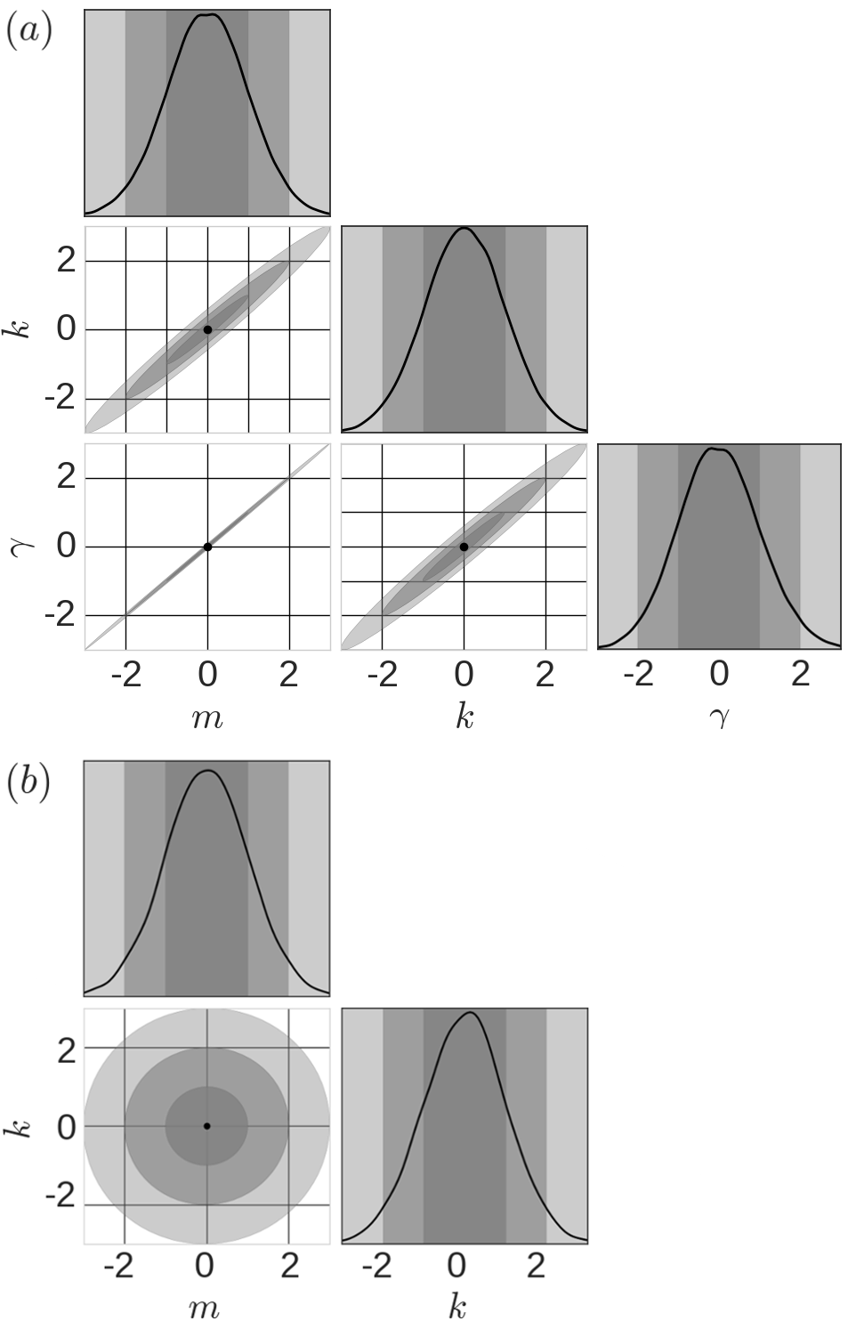
Figure 1: Corner plots of the joint posterior distribution of the mass $m$, friction $\gamma$ and stiffness $k$. Panel $(a)$ shows Bayes I, Eq.(26) while panel $(b)$ shows Bayes II, Eq.(46). The variables have been scaled as $\left(x_{i}-\mu_{{}_{i}}\right)/\sigma_{{}_{ii}}$, where $\mu_{i}$ and $\sigma_{ii}^{2}$ are the MAP estimate and variance of $x_{i}$ respectively. The MAP estimate is marked by a black dot, and the regions of $70\%$, $95\%$ and $99\%$ posterior probability have been shaded.

Next we use Eq.(39) for the covariance matrix in the bivariate analog of Eq.(28) for the logarithm of the posterior probability. The MAP estimates and the error bars for mass $m$ and spring constant $k$ are then

$$\dfrac{k^{\ast}}{k_{B}T}=\dfrac{N}{\sum_{n=1}^{N}x_{n}^{2}} ,\qquad\sigma_{k}=\frac{\sqrt{2}}{\sqrt{N}}k^{\ast},$$ (46a)

$$\dfrac{m^{\ast}}{k_{B}T}=\dfrac{N}{\sum_{n=1}^{N}v_{n}^{2}}, \qquad\,\,\sigma_{m}=\frac{\sqrt{2}}{\sqrt{N}}m^{\ast}.$$ (46b)

These correspond to Bayes II estimates of the oscillator parameters.

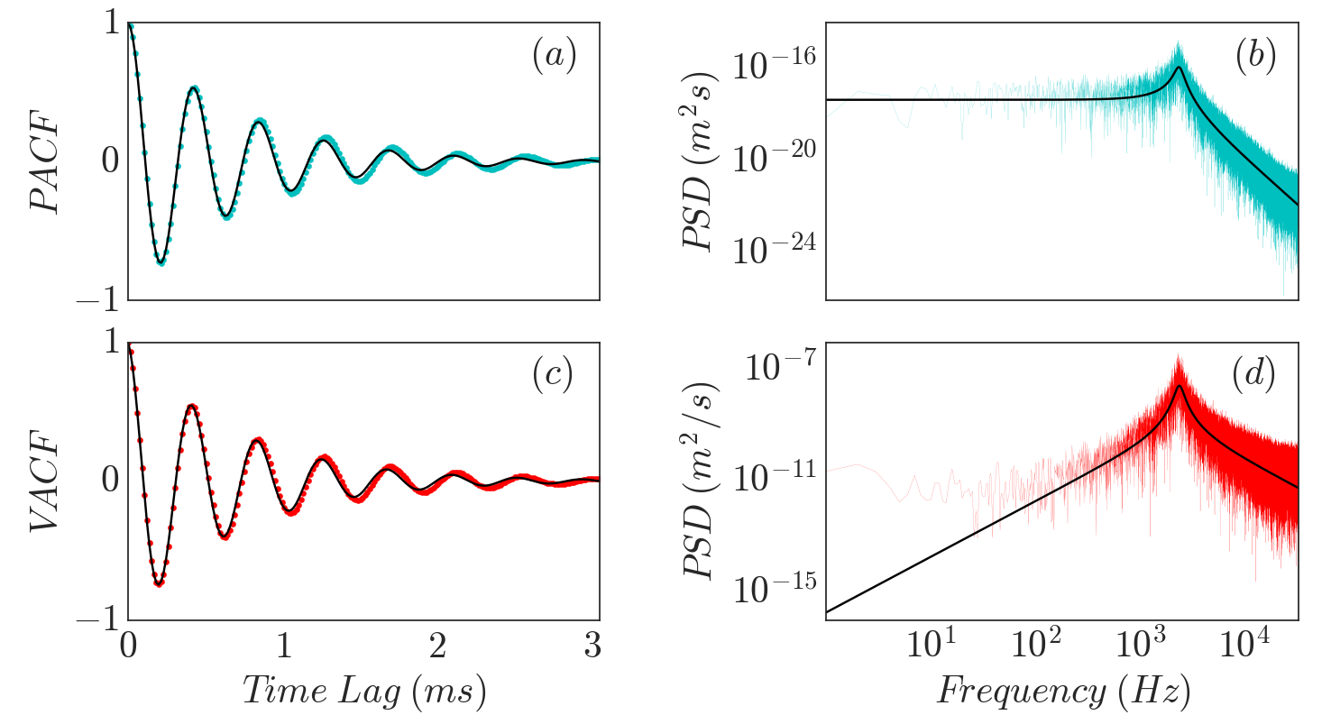
Figure 2: Bayesian estimates of the autocorrelation function and spectral density of position are shown in (a) and (b) respectively as solid lines. There is excellent agreement with simulations shown in cyan. Corresponding estimates for the velocity are shown in (c) and (d) with simulations shown in red.

In Table 1, we provide the MAP estimates and corresponding error bars for three different time-series data obtained from the simulation of the underdamped Brownian harmonic oscillator. This clearly shows that the MAP estimates of both Bayesian methods and values of the simulation parameters are in excellent agreement. The error bars have been calculated from the Hessian matrix. The Bayesian standard error in estimating the parameters is less than $1\%$ for each case.

In Fig.(1) we show the posterior distribution of the parameters as corner plots foreman2016corner , with panel (a) corresponding to Bayes I and panel (b) to Bayes II. The distributions have been shifted to the MAP estimates, which, therefore are always at the origin marked by the black dot, and scaled by the variances. The Bayesian credible intervals corresponding to $70\%$, $95\%$, and $99\%$ of the posterior probability are shown in shades of gray.

Correlation functions and spectral densities: The MAP estimates of the parameters provide a novel way of estimating the correlation functions and spectral densities. Their expressions can be obtained from Eq.(7) and Eq.(8) using the explicit forms of the covariance and the regression matrices. The autocorrelations are

$$\langle x\left(t\right)x\left(0\right)\rangle= \dfrac{k_{B}T}{k}\exp\left(\dfrac{-t}{2\tau}\right)\dfrac{(2\omega\tau\cos\omega t+\sin\omega t)}{2\omega\tau},$$

$$\langle v\left(t\right)v\left(0\right)\rangle= \dfrac{k_{B}T}{m}\exp\left(\dfrac{-t}{2\tau}\right)\dfrac{(2\omega\tau\cos\omega t-\sin\omega t)}{2\omega\tau}.$$

and the spectral densities are

$$C_{xx}(\Omega)= \dfrac{2\gamma k_{B}T}{m^{2}(\omega_{0}^{2}-\Omega^{2})^{2}+\gamma^{2}\Omega^{2}},$$ (47a)

$$C_{vv}(\Omega)= \dfrac{2\gamma k_{B}T\Omega^{2}}{m^{2}(\omega_{0}^{2}-\Omega^{2})^{2}+\gamma^{2}\Omega^{2}}.$$ (47b)

These expressions are evaluated at the Bayesian MAP estimates for the parameters. In Fig.(2), the result is compared with the autocorrelation function and the discrete Fourier transform of the time series. There is excellent agreement between the two autocorrelations. We emphasize that no numerical function fitting is required to obtain this estimate. The spectral density is, arguably, even more impressive as it interpolates through the noisy discrete Fourier transform in a sensible manner. Our estimation of the spectral density shares a methodological similarity with Burg’s classic maximum-entropy method burg1967maximum . The principal differences are (i) that we choose the Ornstein-Uhlenbeck process as the data generating model, rather than the discrete autoregressive process assumed by Burg and (ii) that we work directly on the space of trajectories rather than in the space of correlations. From a Bayesian perspective, our estimation procedure encodes the prior information that the data are generated by an Ornstein-Uhlenbeck process and, therefore, will outperform all methods berg2004power ; tassieri2012microrheology that do not incorporate this prior information, such as the one in Bera:16 .

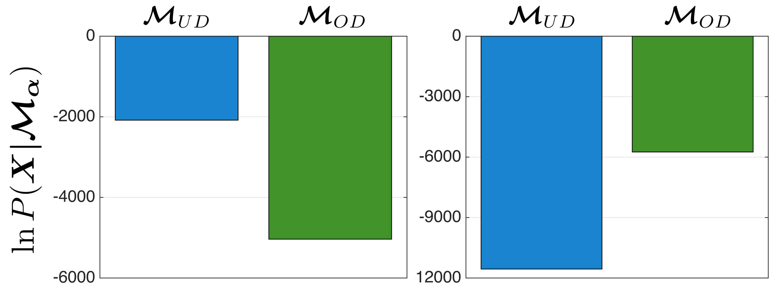
Figure 3: Bayesian model selection procedure for time series data from underdamped ($\mathcal{M}_{UD}$) and overdamped ($\mathcal{M}_{OD}$) Brownian harmonic oscillator. The logarithm of Bayesian evidence has been plotted in the natural log units (nits). The plot for underdamped data $(\gamma=\gamma_{c}/10)$ is shown on the left, while the right panel is for overdamped data $(\gamma=10\gamma_{c})$.

Model comparison: To observe the inertial motion of a colloidal particle in an optical trap, it is necessary to observe the motion at time intervals much smaller than the momentum relaxation time, that is, to ensure $\Delta t\ll\tau$. In the opposite limit, of $\Delta t\gg\tau$, the inertia of the colloid is no longer relevant, and only purely diffusive motion can be observed. These correspond, respectively, to the Kramers and Smoluchowski limits of the Brownian harmonic oscillator. In experiment, it is often not a priori clear if the observational time scale places the system in the Kramers, Smoluchowski, or crossover regime. A Bayesian model comparison provides a principled way to answer this question, as we show below.

We consider two Ornstein-Uhlenbeck data generating models

$$\mathcal{M}_{UD}:\longrightarrow \quad m\dot{v}+\gamma v+\nabla U=\xi$$

$$\mathcal{M}_{OD}:\longrightarrow \quad\gamma\dot{x}+\nabla U=\xi$$ (48)

corresponding, respectively, to motion on the Kramers (underdamped) and Smoluchowski (overdamped) time scales. The latter is the formal $m\rightarrow 0$ limit of Eq.(34) and can be obtained systematically by adiabatically eliminating the velocity as a fast variable gardiner1984adiabatic . The overdamped oscillator is an univariate Ornstein-Uhlenbeck model with two parameters, $\gamma$ and $k$, and Bayesian parameter estimation for it was presented in bera2017fast . The two-parameter overdamped model is simpler than the three-parameter underdamped model. The question we try to answer is which of these models provides the best explanation of the data for the least number of parameters.

To do so, we compare the posterior probability of the model, given the data, by approximating the model evidence in terms of the maximum likelihood and the Ockham factors, assuming equal prior probabilities for the models as in section III. The evidence for both models is straightforwardly computed from the general expression in the Appendix B. For the overdamped model the sufficient statistics are the scalars

$$T_{1} =\sum_{n=1}^{N-1}x_{n+1}^{2},\,\,T_{2}=\sum_{n=1}^{N-1}x_{n+1}x_{n},\,\,T_{3}=\sum_{n=1}^{N-1}x_{n}^{2}.$$ (49)

as was first pointed out in bera2017fast .

In Fig.(3), we plot the logarithm of the Bayesian evidence $\ln P(\boldsymbol{X}|\mathcal{M}_{\alpha})$ in natural log units (nits) for overdamped and underdamped Brownian motion. The panel on the left contains the plot of the logarithm of the evidence for underdamped data while the right panel is for overdamped data. The comparison of $\ln P(\boldsymbol{X}|\mathcal{M}_{\alpha})$ for the overdamped and underdamped models clearly shows that the evidence is greater in each case for the true model of the data.

VI Summary

In summary, we have presented two Bayesian methods for inferring the parameters of a multivariate Ornstein-Uhlenbeck process, given discrete observations of the sample paths. An exact path sampling procedure has been presented and utilized to validate the Bayesian methods for the Brownian harmonic oscillator. The problem of Bayesian model comparison has been addressed and applied to select between Kramers and Smoluchowski limits of the Brownian harmonic oscillator. Future work will address the problem of parameter inference and model selection when either or both of the Markov and Gaussian properties of the process are relaxed.

Appendix A MAP estimates

In this appendix, we make explicit the derivation of Eq.(24) from Eq.(23). To this end, we consider the quadratic form $\boldsymbol{\Delta}_{n}^{\text{tr}}\bm{\Sigma^{-1}\Delta_{n}}=\left(\bm{x_{n+1}}-\bm{\Lambda}\bm{x_{n}}\right)^{\text{tr}}\bm{\Sigma^{-1}}\left(\bm{x_{n+1}}-\bm{\Lambda}\bm{x_{n}}\right)$ that occurs in the expression of the logarithm of the posterior probability in Eq.(23). Expanding terms and completing the summation we have the following identity

$$-\frac{1}{2}\sum_{n=1}^{N-1}\boldsymbol{\Delta}_{n}^{\text{tr}}\bm{\Sigma^{-1}\Delta_{n}}=-\dfrac{1}{2}\bm{\Sigma}^{-1}:\Big{[}\left(\bm{\Lambda}-\bm{T_{2}T_{3}^{-1}}\right)\left(\bm{T_{3}}\right)\left(\bm{\Lambda}-\bm{T_{2}T_{3}^{-1}}\right)^{\text{tr}}+\left(\bm{T}_{1}-\bm{T}_{2}\bm{T}_{3}^{-1}\bm{T}_{2}^{\text{tr}}\right)\Big{]}.$$ (50)

Here, we have used the definitions of sufficient statistics in Eq.(25). With this identification, the expression of the logarithm of the posterior probability in terms of the sufficient statistics is given in Eq.(24). Inspecting the expression, we recognize that the posterior is normal in $\boldsymbol{\Lambda}$ which directly yields its MAP estimate $\boldsymbol{\Lambda}^{*}=\bm{T}_{2}\bm{T}_{3}^{-1}$. Taking the derivative of the above equation with respect to $\boldsymbol{\Sigma}^{-1}$ and using the matrix identity $\partial\ln\left(\det\bm{A}\right)/\partial\bm{A}=\left(\bm{A}^{\text{tr}}\right)^{-1}$, we obtain

$$\dfrac{\partial\ln P\left(\bm{\theta}|\bm{X}\right)}{\partial\bm{\Sigma^{-1}}}=-\dfrac{1}{2}\Big{[}\left(\bm{\Lambda}-\bm{T}_{2}\bm{T}_{3}^{-1}\right)\left(\bm{T}_{3}\right)\left(\bm{\Lambda}-\bm{T}_{2}\bm{T}_{3}^{-1}\right)^{\text{tr}}+\left(\bm{T}_{1}-\bm{T}_{2}\bm{T}_{3}^{-1}\bm{T}_{2}^{\text{tr}}\right)\Big{]}+\dfrac{N}{2}\bm{\Sigma}.$$ (51)

At the maximum, we obtain the MAP estimate as $\bm{\Sigma^{\ast}}=\dfrac{1}{N}\left(\bm{T}_{1}-\boldsymbol{T}_{2}\boldsymbol{T}_{3}^{-1}\boldsymbol{T}_{2}^{\text{tr}}\right).$ The estimates of the parameters of the underdamped oscillator follow from $\bm{\Lambda^{\ast}}$ and $\bm{\Sigma^{\ast}}$ after algebraic manipulations, see Appendix of rasmussen2006gaussian for further details.

Appendix B Standard errors and evidence

We now obtain an explicit expression for the standard errors and evidence from the derivatives of the logarithm of the posterior distribution. The second partial derivatives of the logarithm of the posterior distribution with respect to $\boldsymbol{\Sigma}^{-1}$ and $\boldsymbol{\Lambda}$, at the maximum, are

$$\dfrac{\partial^{2}\ln P\left(\bm{\theta}|\bm{X}\right)}{\partial(\bm{\Sigma^{-1}})^{2}}= -\dfrac{N}{2}\left(\bm{\Sigma}^{*}\right)^{2},$$ (52a)

$$\dfrac{\partial^{2}\ln P\left(\bm{\theta}|\bm{X}\right)}{\partial\bm{\Lambda}^{2}}= -\bm{\Sigma}^{*-1}(\bm{T_{3}}+N\boldsymbol{c}*)-\frac{N}{2}\bm{\Sigma}^{*-2}((\bm{\Lambda}^{*}\boldsymbol{c}^{*}+\boldsymbol{c}^{*}\bm{\Lambda}^{*\text{tr}}))^{2}.$$ (52b)

The mixed partial derivative at the maximum is

$$\dfrac{\partial^{2}\ln P\left(\bm{\theta}|\bm{X}\right)}{\partial\bm{\Lambda}\partial\bm{\Sigma^{-1}}} \eqsim-\frac{N}{2}(\bm{\Lambda}^{*}\boldsymbol{c}^{*}+\boldsymbol{c}^{*}\bm{\Lambda}^{*\text{tr}}).$$ (53)

The Hessian matrix, $\boldsymbol{A}=-\nabla\nabla\ln P\left(\bm{\theta}|\bm{X}\right)$, at the maximum is then

$$\boldsymbol{A}=\left(\begin{array}[]{ccc}\tfrac{N}{2}(\bm{\Sigma}^{*})^{2}&&\frac{N}{2}(\bm{\Lambda}^{*}\boldsymbol{c}^{*}+\boldsymbol{c}^{*}\bm{\Lambda}^{*\text{tr}})\\ &\\ \frac{N}{2}(\bm{\Lambda}^{*}\boldsymbol{c}^{*}+\boldsymbol{c}^{*}\bm{\Lambda}^{*\text{tr}})&&\bm{\Sigma}^{*-1}(\bm{T_{3}}-N\boldsymbol{c}^{*})-\frac{N}{2}\bm{\Sigma}^{*-2}(\bm{\Lambda}^{*}\boldsymbol{c}^{*}+\boldsymbol{c}^{*}\bm{\Lambda}^{*\text{tr}})^{2}\end{array}\right).$$ (57)

The above expression of the Hessian matrix has been used to obtain the standard errors of the MAP estimates and the evidence of a given model.

The expression of the Bayesian evidence of a model $\mathcal{M}_{\alpha}$ with several parameters is given in terms of the likelihood and the Hessian matrix as mackay2003information

$$P(\boldsymbol{X}|\mathcal{M}_{\alpha})\simeq P(\boldsymbol{X}|\boldsymbol{\theta}^{\ast},\mathcal{M}_{\alpha})\,P(\boldsymbol{\theta}^{\ast}|\mathcal{M}_{\alpha})[\det(\bm{A}/2\pi)]^{-1/2}.$$ (58)

This expression has been used to obtain the logarithm of the evidence for a $M$-dimensional multivariate Ornstein-Uhlenbeck model $\mathcal{M}_{\alpha}$. Using explicit forms of the likelihood and the Hessian matrix, at the maximum, the expression of the logarithm of the evidence for a model $\mathcal{M}_{\alpha}$ is given as

$$\ln P\left(\bm{X}|\mathcal{M}_{\alpha}\right) \simeq-\frac{N}{2}\left(\bm{\Sigma}^{*^{-1}}:\bm{\Sigma}^{*}+\ln((2\pi)^{M}\,|\bm{\Sigma}^{*}|)\right)-\frac{1}{2}\ln\Big{(}\det(\boldsymbol{A}_{22})\det(\boldsymbol{A}_{11}-\boldsymbol{A}_{12}\boldsymbol{A}_{22}^{-1}\boldsymbol{A}_{21})\Big{)}+\tfrac{M}{2}\ln 2\pi.$$ (59)

Here $\boldsymbol{A}_{ij}$ are the elements of the Hessian matrix.

Appendix C Path sampling

In this appendix, we provide explicit expressions for $e^{-\boldsymbol{\lambda}\Delta t}$ and $\sqrt{\boldsymbol{\Sigma}}$, needed for the path sampling of a bivariate Ornstein-Uhlenbeck process in section V. From the Cayley-Hamilton theorem, $e^{-\boldsymbol{\lambda}\Delta t}$ is obtained in terms of the identity matrix and $\boldsymbol{\lambda}$ as shown in Eq.(40). The coefficients are

$$\Lambda_{1} = \exp(\tfrac{-\Delta t}{2\tau})\left[\cos(\omega\Delta t)+\frac{1}{2\omega\tau}\sin(\omega\Delta t)\right],$$ (60a)

$$\Lambda_{2} = \exp(\tfrac{-\Delta t}{2\tau})\left[-\frac{1}{\omega}\sin(\omega\Delta t)\right].$$ (60b)

Here $\omega=\sqrt{\omega_{0}^{2}-1/(2\tau)^{2}}$ is the frequency of the damped oscillator. $\sqrt{\boldsymbol{\Sigma}}$ is obtained from its Cholesky factorization into a lower triangular matrix and its transpose, as shown in Eq.(41). The elements of the Cholesky factor are

$$s_{1} =\bigg{[}\frac{k_{B}T}{k}-\frac{k_{B}T}{k}\exp(\tfrac{-\Delta t}{\tau})\Big{(}\frac{k}{m\omega^{2}}\sin^{2}(\omega\Delta t)+\big{[}\cos(\omega\Delta t)+\tfrac{1}{2\omega\tau}\sin(\omega\Delta t)\big{]}^{2}\Big{)}\bigg{]}^{1/2},$$ (61a)

$$s_{2} =\frac{1}{s_{1}}\dfrac{k_{B}T}{\gamma\omega^{2}\tau^{2}}\exp(\tfrac{-\Delta t}{\tau})\sin^{2}(\omega\Delta t),$$ (61b)

$$s_{3} =\bigg{[}\frac{k_{B}T}{m}-\frac{k_{B}T}{m}\exp(\tfrac{-\Delta t}{\tau})\Big{(}\frac{k}{m\omega^{2}}\sin^{2}(\omega\Delta t)+\big{[}\cos(\omega\Delta t)-\tfrac{1}{2\omega\tau}\sin(\omega\Delta t)\big{]}^{2}\Big{)}-s_{2}^{2}\bigg{]}^{1/2}.$$ (61c)

We use the above to elucidate the results in Eq.(33) in order to obtain exactly sampled trajectories of the Brownian harmonic oscillator. In Fig.(4) we show a typical sample path of the positions and velocities and their corresponding histograms. The histograms of the positions and the velocities clearly show that the distributions are normal.

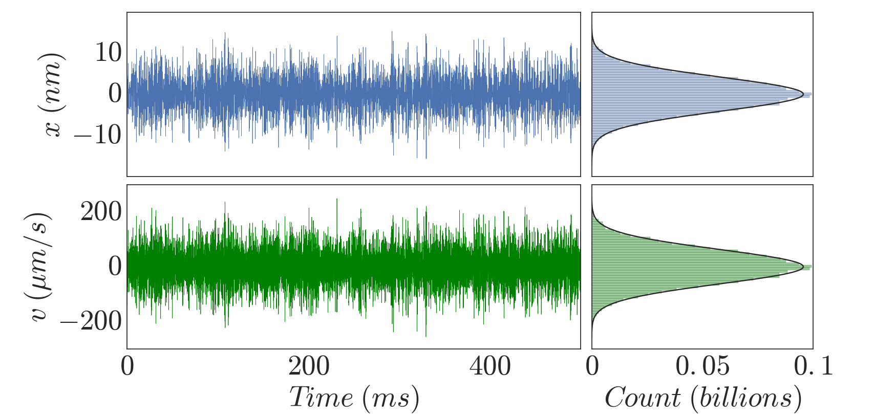
Figure 4: Sample paths (left) and histograms (right) of the position and velocity of the Brownian harmonic oscillator obtained from exact path sampling, Eq. (33). Parameters used are$m=1ng$, $k=225mg/s^{2}$, $\gamma=\gamma_{c}/10$, $\gamma_{c}=\sqrt{4mk}$ and $T=275K$. The path is sampled at $2^{16}Hz$.

References

- (1) J. L. Doob. The Brownian movement and stochastic equations. Ann. Math., pages 351–369, 1942.
- (2) J. L. Doob. Stochastic processes, volume 7. Wiley New York, 1953.
- (3) N. G. van Kampen. Stochastic processes in physics and chemistry. Elsevier, 1992.
- (4) C. W. Gardiner. Handbook of stochastic methods. Springer Berlin, 1985.
- (5) D. J. C. MacKay. Information theory, inference and learning algorithms. Cambridge University Press, 2003.
- (6) C. E. Rasmussen and C. K. I. Williams. Gaussian processes for machine learning, volume 1. MIT press Cambridge, 2006.
- (7) F. Lindgren, H. Rue, and J. Lindström. An explicit link between Gaussian fields and Gaussian Markov random fields: the stochastic partial differential equation approach. J. Royal Stat. Soc.: Series B (Stat. Meth.), 73(4):423–498, 2011.
- (8) A. J. Smola and B. Schölkopf. Sparse greedy matrix approximation for machine learning. pages 911–918. Morgan Kaufmann, San Francisco, 2000.
- (9) C. K. I. Williams and M. Seeger. Using the Nyström method to speed up kernel machines. In Advances in neural information processing systems, pages 682–688. MIT press, 2001.
- (10) L. Csató and M. Opper. Sparse on-line Gaussian processes. Neur. Comp., 14(3):641–668, 2002.
- (11) J. Quiñonero-Candela and C. E. Rasmussen. A unifying view of sparse approximate Gaussian process regression. J. Mach. Learn. Res., 6:1939–1959, 2005.
- (12) A. Kavcic and J. M. F. Moura. Matrices with banded inverses: Inversion algorithms and factorization of Gauss-Markov processes. IEEE Trans. Inf. Theory, 46(4):1495–1509, 2000.
- (13) H. Jeffreys. The theory of probability. Oxford University Press, Oxford, 1939.
- (14) E. T. Jaynes. Probability theory: The logic of science. Cambridge University Press, 2003.
- (15) D. Sivia and J. Skilling. Data analysis: a Bayesian tutorial. Oxford University Press, Oxford, 2006.
- (16) S. Bera, S. Paul, R. Singh, D. Ghosh, A. Kundu, A. Banerjee, and R. Adhikari. Fast Bayesian inference of optical trap stiffness and particle diffusion. Sci. Rep., 7:41638, 2017.
- (17) R. Kashyap. A bayesian comparison of different classes of dynamic models using empirical data. IEEE Trans. Automat. Cont., 22(5):715–727, 1977.
- (18) D. J. C. MacKay. Bayesian interpolation. Neur. Computn., 4:415–447, 1992.
- (19) A. Zellner. Basic Issues in Econometrics. University of Chicago Press, Chicago, 1984.
- (20) P. Gregory. Bayesian Logical Data Analysis for the Physical Sciences. Cambridge University Press, 2005.
- (21) G. E. Uhlenbeck and L. S. Ornstein. On the theory of the Brownian motion. Phys. Rev., 36(5):823, 1930.
- (22) A. Parker and C. Fox. Sampling Gaussian distributions in Krylov spaces with conjugate gradients. SIAM J. Sci. Comput., 34(3):B312–B334, 2012.
- (23) S. Chandrasekhar. Stochastic problems in physics and astronomy. Rev. Mod. Phys., 15:1–89, 1943.
- (24) A. Einstein. The theory of the Brownian movement. Ann. Phys. (Berlin), 322:549, 1905.
- (25) R. Kubo. The fluctuation-dissipation theorem. Rep. Prog. Phys., 29(1):255, 1966.
- (26) D. Foreman-Mackey. corner.py: Scatterplot matrices in Python. The Journal of Open Source Software, 1(2):1–2, 2016.
- (27) J. P. Burg. Maximum entropy spectral analysis. PhD thesis, Stanford University, 1975.
- (28) K. Berg-Sørensen and H. Flyvbjerg. Power spectrum analysis for optical tweezers. Rev. Sci. Inst., 75(3):594–612, 2004.
- (29) M. Tassieri, R. Evans, R. L. Warren, N. J. Bailey, and J. M. Cooper. Microrheology with optical tweezers: data analysis. New J. Phys., 14(11):115032, 2012.
- (30) S. Bera, A. Kumar, S. Sil, T. K. Saha, T. Saha, and A. Banerjee. Simultaneous measurement of mass and rotation of trapped absorbing particles in air. Opt. Lett., 41(18):4356–4359, 2016.
- (31) C. W. Gardiner. Adiabatic elimination in stochastic systems. I. Formulation of methods and application to few-variable systems. Phys. Rev. A, 29(5):2814–2822, 1984.