Numerical Simulation of the SVS 13
Micro-Jet and Bow Shock Bubble

Abstract

Numerical simulations are performed using the WENO method of the SVS 13 micro-jet and bow shock bubble which reproduce the main features and dynamics of Keck Telescope/OSIRIS velocity-resolved integral field spectrograph data: an expanding cooler bow shock bubble, with the bubble center moving at approximately 50 km s^-1 with a radial expansion velocity of 11 km s^-1, surrounding the fast hotter jet, which is propagating at 156 km s^-1. Contact and bow shock waves are visible in the simulations from both the initial short jet pulse which creates the nearly spherical bow shock bubble and from the fast micro-jet, while a terminal Mach disk shock is visible near the tip of the continuous micro-jet, which reduces the jet gas velocity down to the flow velocity of the contact discontinuity at the leading edge of the jet. At 21.1 yr after the launch of the initial bubble pulse, the jet has caught up with and penetrated almost all the way across the bow shock bubble of the slower initial pulse. At times later than about 22 yr, the jet has penetrated through the bubble and thereafter begins to subsume its spherical form. Emission maps from the simulations of the jet—traced by the emission of the shock excited 1.644 $\mu$m [Fe II] line—and bow shock bubble—traced in the lower excitation 2.122 $\mu$m H₂ 1–0 S(1) line—projected onto the plane of the sky are presented, and are in good agreement with the Keck observations.

1 Introduction

Keck Telescope laser adaptive-optics integral field spectroscopy with OSIRIS by Hodapp & Chini (2014) of the innermost regions of the NGC 1333 SVS 13 outflow (which forms the system of Herbig-Haro objects 7–11) revealed a bright micro-jet traced by the emission of shock excited [Fe II]. In addition, a series of bow shock bubbles and fragments of bubbles beyond this micro-jet were observed in the lower excitation H₂ 1–0 S(1) line.

The kinematic age of the youngest bubble is slightly older than the last observed photometric outburst of SVS 13 in 1990, and consistent with that event launching the bubble with some subsequent deceleration of its expansion.

Jet outflows emanating from young stars typically are comprised of a series of individual shock fronts that arise from changes in the jet velocity as a result of repetitive eruptive events (see the review by Reipurth & Bally (2001) and references therein). This general framework can be applied to SVS 13: the FUor-like photometric outburst in 1990 produced a short-lived pulse of jet activity which formed a bow shock bubble as it ran into slower moving material ejected prior to the outburst event. Subsequent to the formation of the bubble, the SVS 13 stellar source ejected a fast continuous micro-jet that caught up with and pierced the bubble, partially incorporating and destroying the bubble. In SVS 13, this process is currently repeating itself about every 30 yr, creating the series of bubble fragments that make up the string of Herbig-Haro objects.

The creation of a series of bubbles and the changes in outflow direction indicate that the accretion disk of SVS 13 is precessing. The 30 yr cycle of bubble pulses may correspond with the orbit of an as yet unobserved close binary companion, and/or to revolving inhomogeneities in the accretion disk.

In this investigation, we present the first numerical simulations of the SVS 13 micro-jet and most recent bow shock bubble, using the WENO method. These simulations reproduce the main features and dynamics of the Keck data: an expanding cooler bow shock bubble, with the bubble center moving at approximately 50 km s^-1 with a radial expansion velocity of 11 km s^-1, surrounding the fast hotter jet, which is propagating at 156 km s^-1. Emission maps from the simulations of the jet—traced by the emission of the shock excited 1.644 $\mu$m [Fe II] line—and bow shock bubble—traced in the lower excitation 2.122 $\mu$m H₂ 1–0 S(1) line— projected onto the plane of the sky are also presented, and are in good agreement with the Keck observations.

The only other known examples of a young stellar object outflow with pronounced bubble structures are XZ Tauri (Krist et al. 2008) and IRAS 16293–2422 (Loinard et al. 2013). The first numerical simulations of bow shock bubbles originated and penetrated by jet pulses (in XZ Tauri) were presented in Krist et al. (2008) and Gardner & Dwyer (2009), using our WENO code. These simulations modeled a faster, more rapidly pulsing proto-jet which produced more rapidly expanding and overlapping bubbles.

2 Numerical Method and Radiative Cooling

We applied the WENO method—a modern high-order upwind method—to simulate the expanding bow shock bubble and jet in SVS 13, including the effects of atomic and molecular radiative cooling.

We use a third-order WENO (weighted essentially non-oscillatory) method (Shu 1999) for the simulations (Ha et al. 2005). ENO and WENO schemes are high-order finite difference schemes designed for nonlinear hyperbolic conservation laws with piecewise smooth solutions containing sharp discontinuities like shock waves and contacts. Locally smooth stencils are chosen via a nonlinear adaptive algorithm to avoid crossing discontinuities whenever possible in the interpolation procedure. The weighted ENO (WENO) schemes use a convex combination of all candidate stencils, rather than just one as in the original ENO method.

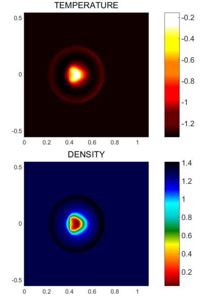
Figure 2: Cross section of the numerical simulation of the SVS 13 bow shock bubble at 18.5 yr (circa 2008), just before the fast jet is turned on: logarithm of temperature $\log_{10}\left(T/\overline{T}\right)$, where $\overline{T}$ = $10^{4}$ K, and logarithm of density $\log_{10}\left(\rho/\overline{\rho}\right)$, where $\overline{\rho}$ = 100 H cm^-3. Lengths along the left and bottom boundaries are in $10^{10}$ km for Figures 2–13. Note that all simulation images are more or less zoomed in.

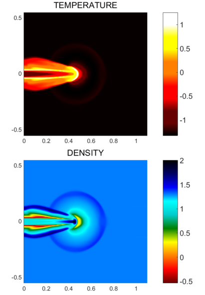
Figure 3: Cross section of the numerical simulation of the SVS 13 bow shock bubble and jet at 20.4 yr (circa 2010): logarithm of temperature $\log_{10}\left(T/\overline{T}\right)$, where $\overline{T}$ = $10^{4}$ K, and logarithm of density $\log_{10}\left(\rho/\overline{\rho}\right)$, where $\overline{\rho}$ = 100 H cm^-3. Lengths are in $10^{10}$ km.

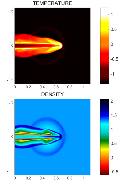
Figure 4: Cross section of the numerical simulation of the SVS 13 bow shock bubble and jet at 21.1 yr (circa 2011): logarithm of temperature $\log_{10}\left(T/\overline{T}\right)$, where $\overline{T}$ = $10^{4}$ K, and logarithm of density $\log_{10}\left(\rho/\overline{\rho}\right)$, where $\overline{\rho}$ = 100 H cm^-3. Lengths are in $10^{10}$ km.

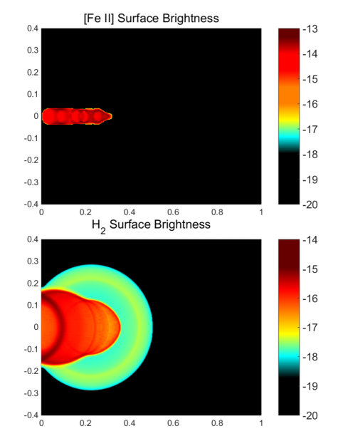
Figure 5: Simulated surface brightness $S$ in the 1.644 $\mu$m [Fe II] line and the 2.122 $\mu$m H₂ line of the SVS 13 jet and bow shock bubble at 21.1 yr (circa 2011): $\log_{10}(S)$ with $S$ in erg cm^-2 arcsec^-2 s^-1. The jet and bubble have been projected with a declination angle of 30^∘ with respect to the line of sight. Lengths are in $10^{10}$ km.

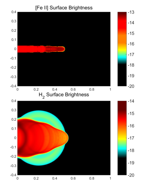
Figure 7: Simulated surface brightness $S$ in the 1.644 $\mu$m [Fe II] line and the 2.122 $\mu$m H₂ line of the SVS 13 jet and bow shock bubble at 22.3 yr (circa 2012): $\log_{10}(S)$ with $S$ in erg cm^-2 arcsec^-2 s^-1. The jet and bubble have been projected with a declination angle of 30^∘ with respect to the line of sight. Lengths are in $10^{10}$ km.

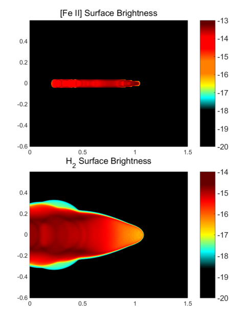
Figure 9: Simulated surface brightness $S$ in the 1.644 $\mu$m [Fe II] line and the 2.122 $\mu$m H₂ line of the SVS 13 jet and bow shock bubble at 26.1 yr (circa 2016): $\log_{10}(S)$ with $S$ in erg cm^-2 arcsec^-2 s^-1. The jet and bubble have been projected with a declination angle of 30^∘ with respect to the line of sight. Lengths are in $10^{10}$ km.

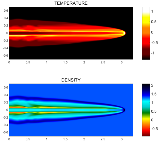
Figure 10: Cross section of the numerical simulation of the SVS 13 bow shock bubble and jet at 30 yr (circa 2020), assuming the jet source has not turned off: logarithm of temperature $\log_{10}\left(T/\overline{T}\right)$, where $\overline{T}$ = $10^{4}$ K, and logarithm of density $\log_{10}\left(\rho/\overline{\rho}\right)$, where $\overline{\rho}$ = 100 H cm^-3. Lengths are in $10^{10}$ km.

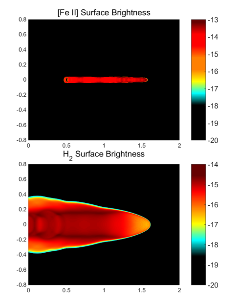
Figure 11: Simulated surface brightness $S$ in the 1.644 $\mu$m [Fe II] line and the 2.122 $\mu$m H₂ line of the SVS 13 jet and bow shock bubble at 30 yr (circa 2020): $\log_{10}(S)$ with $S$ in erg cm^-2 arcsec^-2 s^-1. The jet and bubble have been projected with a declination angle of 30^∘ with respect to the line of sight. Lengths are in $10^{10}$ km.

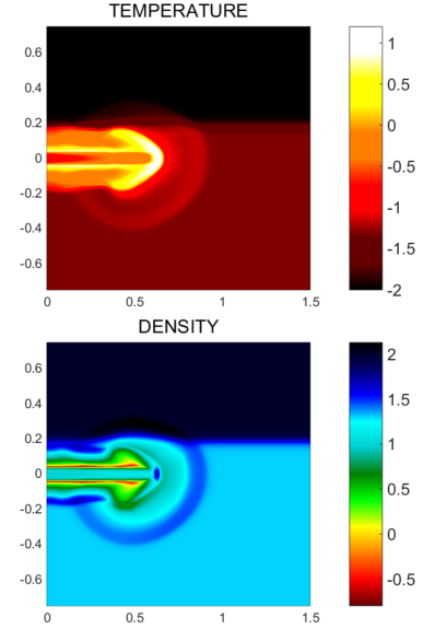
Figure 12: Cross section of the numerical simulation of the SVS 13 bow shock bubble and jet at 21 yr with a heavier ambient (5 times the usual $\rho_{a}$) “above” the jet: logarithm of temperature $\log_{10}\left(T/\overline{T}\right)$, where $\overline{T}$ = $10^{4}$ K, and logarithm of density $\log_{10}\left(\rho/\overline{\rho}\right)$, where $\overline{\rho}$ = 100 H cm^-3. Lengths are in $10^{10}$ km.

Our WENO code is parallelized using OpenMP and MPI, and can simulate both cylindrically symmetric flows (Figures 2–11 below) as well as fully three-dimensional flows (Figures 12 and 13).

The equations of gas dynamics with radiative cooling take the form of hyperbolic conservation laws for mass, momentum, and energy:

$$\frac{\partial\rho}{\partial t}+\frac{\partial}{\partial x_{i}}(\rho u_{i})=0$$ (1)

$$\frac{\partial}{\partial t}(\rho u_{j})+\frac{\partial}{\partial x_{i}}(\rho u_{i}u_{j})+\frac{\partial P}{\partial x_{j}}=0$$ (2)

$$\frac{\partial E}{\partial t}+\frac{\partial}{\partial x_{i}}(u_{i}(E+P))=-C(n,T)$$ (3)

where $\rho=mn$ is the density of the gas, $m$ is the mass of the gas atoms or molecules (largely either $m_{H}$ or $2m_{H}$ where $m_{H}$ is the mass of H), $n$ is the number density, $u_{i}$ is the velocity, $\rho u_{i}$ is the momentum density, $P=nk_{B}T$ is the pressure, $k_{B}$ is Boltzmann’s constant, $T$ is the temperature, and

$$E=\frac{3}{2}nk_{B}T+\frac{1}{2}\rho u^{2}$$ (4)

is the energy density. Indices $i,~{}j$ equal 1, 2, 3, and repeated indices are summed over.

Radiative cooling of the gas is incorporated through the right-hand side $-C(n,T)$ of the energy conservation equation (3), where

$$C(n,T)=\left\{\begin{array}[]{ll}n^{2}\Lambda(T)&T\geq 8000~{}{\rm K,~{}atomic~{}cooling~{}only}\\ nW(n,T)&100~{}{\rm K}\leq T<8000~{}{\rm K,~{}H}_{2}~{}{\rm cooling~{}only}\\ \end{array}\right.$$ (5)

with the model for $\Lambda(T)$ taken from Figure 8 of Schmutzler & Tscharnuter (1993) for atomic cooling (encompassing the relevant emission lines of the ten most abundant elements H, He, C, N, O, Ne, Mg, Si, S, and Fe in the interstellar medium (ISM), as well as relevant continuum processes) and the model for $W(n,T)$ from Figure 4 of Le Bourlot et al. (1999) for H₂ molecular cooling. In these two references, the cooling functions are calculated in a thermally self-consistent way—not assuming thermal equilibrium—involving detailed energy balancing and time-dependent stages of ionization. $\Lambda(T)$ incorporates sub-dominant heating in addition to dominant cooling. (Both atomic and molecular cooling are actually operative between 8000 K $\leq T\leq$ 10,000 K, but atomic cooling is dominant in this range.) Note that $C(n,T)$ is discontinuous at $T$ = 8000 K; however this does not cause any mathematical or numerical problems, since mathematically the homogeneous gas dynamical equations already support stronger discontinuities (discontinuous shock and contact waves), and since numerically $-C(n,T)$ is integrated over a timestep (not differentiated in time or space).

We assume that the ambient gas (including the cool bow shocked ambient of the bubble) is almost entirely H₂ throughout the simulation, and use part (a) of Figure 4 of Le Bourlot et al. (1999) with $n(H)/n(H_{2})=0.01$. The bubble bow shock running into the stationary ambient molecular hydrogen at 11 km s^-1 is capable of exciting the 1–0 S(1) line emission while not dissociating the H₂ (see for example Draine 1980). We assume that the jet gas and the immediately adjacent, hot, turbulently mixed, bow shocked jet/ambient gas (above 8000 K) are predominantly H, with the standard admixture of the other nine most abundant elements in the ISM.

Below we calculate emission maps from the 2D cylindrically symmetric simulations of the SVS 13 jet and bow shock bubble projected onto the plane of the sky, at a distance of $R$ = 235 pc with a declination angle of 30^∘ with respect to the line of sight. The jet is best traced by the emission of the shock excited 1.644 $\mu$m [Fe II] line, while the bow shock bubble is best traced in the lower excitation 2.122 $\mu$m H₂ 1–0 S(1) line (Hodapp & Chini 2014).

To calculate the 1.644 $\mu$m [Fe II] and 2.122 $\mu$m H₂ emission, we post-processed the computed solutions using emissivities extracted from the astrophysical spectral synthesis package Cloudy (version 13.03, last described by Ferland et al. 2013). For the [Fe II] emission line, we calculated the emissivity $\epsilon_{1.644\mu m}$ as a function of $n$ and $T$. Similarly for the H₂ emission line, we calculated $\epsilon_{2.122\mu m}$ as a function of $n_{H_{2}}$ (assuming that the ambient gas is almost entirely H₂ below 8000 K) and $T$. In practice, we calculated a table of values for $\log_{10}(\epsilon_{line})$ on a grid of $(\log_{10}(n),\log_{10}(T))$ values relevant in the simulations to each line, and then used bilinear interpolation in $\log_{10}(n)$ and $\log_{10}(T)$ to compute $\log_{10}(\epsilon_{line})$.

Surface brightness $S_{line}$ in any emission line is then calculated by integrating along the line of sight through the jet and bubble

$$S_{line}=\frac{\int\epsilon_{line}(n,T)dl}{4\pi R^{2}}$$ (6)

and converting to erg cm^-2 arcsec^-2 s^-1, with $R$ = 235 pc and 20 mas = 4.7 AU for SVS 13. For details and validation of the emission line calculations, see C.L.G., J.R.J., & P. B. Vargas (in preparation).

An alternative approach to ionization effects in radiative cooling of astrophysical jets is outlined in Tesileanu et al. (2014).

3 Numerical Simulations

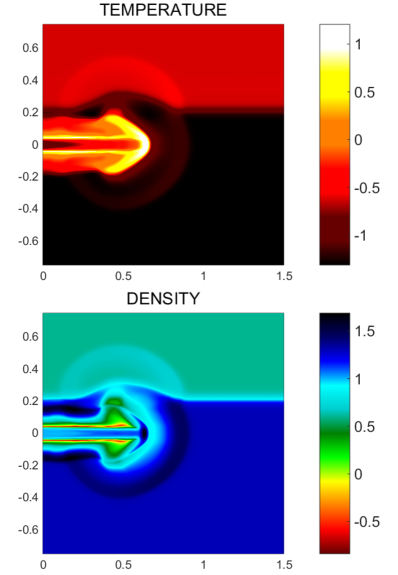
Figure 13: Cross section of the numerical simulation of the SVS 13 bow shock bubble and jet at 21 yr with a lighter ambient (1/5 the usual $\rho_{a}$) “above” the jet: logarithm of temperature $\log_{10}\left(T/\overline{T}\right)$, where $\overline{T}$ = $10^{4}$ K, and logarithm of density $\log_{10}\left(\rho/\overline{\rho}\right)$, where $\overline{\rho}$ = 100 H cm^-3. Lengths are in $10^{10}$ km.

Parallelized simulations of the SVS 13 bow shock bubble and jet were performed on a $1200\Delta z\times 400\Delta r$ grid spanning $3.3\times 10^{10}$ km by $2.2\times 10^{10}$ km (using the cylindrical symmetry) for the cylindrically symmetric simulations in Figures 2–11 and a $500\Delta x\times 500\Delta y\times 750\Delta z$ grid spanning $2\times 10^{10}$ km by $2\times 10^{10}$ km by $3\times 10^{10}$ km for the fully 3D simulations in Figures 12 and 13. The initial bubble pulse and the jet are emitted at the center $(r,z)=(0,0)$ or $(x,y,z)=(0,0,0)$ of the left boundary of the computational grid in Figures 2–13, with a jet diameter of $5\times 10^{8}$ km, propagating to the right along the $z$ axis. All the simulation images in Figures 2–13 are more or less zoomed in, to best display the results.

The Keck Telescope image in Figure 1 shows the jet propagating down and to the left towards the observer at an angle of about 20–30^∘ with respect to the line of sight. The Keck data show an expanding cooler bow shock bubble, with the bubble center moving at approximately 50 km s^-1 with a radial expansion velocity of 11 km s^-1, surrounding the fast hotter jet, which is propagating at 156 km s^-1. In the Keck image, the bubble has a diameter of approximately $10^{10}$ km (reproduced in the simulations). Kinematics then suggests that the bubble is 21 yr old in Figure 1 (imaged in 2011), with its emission corresponding to a photometric outburst of the SVS 13 stellar source in 1990.

Table 1: Parameters for the jet, bow shock bubble, and ambient gas.

jet	bubble pulse	ambient gas
$\rho_{j}$ = 1000 H cm-3	$\rho_{b}$ = 1000 H cm-3	$\rho_{a}$ = 1000 H2 cm-3
$u_{j}$ = 156 km s-1	$u_{b}\approx 50$ km s-1	$u_{a}$ = 0
$T_{j}$ = 1000 K	$T_{b}$ = 1000 K	$T_{a}$ = 500 K
$c_{j}$ = 3.7 km s-1	$c_{b}$ = 3.7 km s-1	$c_{a}$ = 2.6 km s-1

The initial pulse and jet are presumably denser and cooler than the far-field ambient gas, but we believe the pulse and jet are propagating into previous outflows from the star, so they may in fact be less dense and hotter than the near-field ambient wind from the star. For the simulations, we took the pulse and jet to be half as dense as the near-field ambient, and twice as hot. If the pulse that generates the bubble is denser than the ambient, extremely high temperatures are generated ($\gg$ 100,000 K), which disagree with the Keck data. By assuming the bubble and jet are less dense than the immediate ambient gas, temperatures are kept well below 10,000 K for the most part.

In the numerical simulations, the initial thin cylindrical-disk jet pulse of supersonic gas, which creates the nearly spherical bow shock bubble, has a density of 1000 H cm^-3 and a temperature of 1000 K (see Table 1). In the simulations, the center of the bow shock bubble propagates at an average velocity of approximately 50 km s^-1 over the first 23 yr. A short initial pulse of duration 0.08 yr was allowed to propagate for 18.5 yr to form the bow shock bubble (see Figure 2), and then the fast jet was turned on and allowed to propagate to 20.4, 21.1, 22.3, 26.1, and 30 yr respectively in Figures 3–11. (Figures 2–11 show temperature and density cross sections of the simulations in a plane containing the $z$ axis, and surface brightness of the jet and bubble projected onto the plane of the sky.) The jet inflow is propagating at 156 km s^-1, with the same density and temperature as the initial pulse. The jet is surrounded by a strong bow shock plus bow shocked envelope in Figures 3–11. The undisturbed ambient density is 1000 H₂ cm^-3, with a temperature of 500 K, so that the different gases are initially pressure matched. The jet is propagating at Mach 60 with respect to the soundspeed in the heavier ambient gas and Mach 42 with respect to the soundspeed in the jet gas.

The Keck image in Figure 1 shows an asymmetric bow shock bubble, with a much weaker shock on one side (also see Figures 1 and 4 in Hodapp & Chini (2014)). This weakening could be caused by the jet running into heavier and cooler gas from a previous outflow on that side, as in Figure 12. If the previous outflow on that side were lighter and hotter, the bow shock bubble would expand and become hotter, as in Figure 13.

4 Discussion

The surface of the bow shock bubble remains $\sim$ 1000 K throughout the simulations, while some parts of the narrower bow shocked envelope of the jet remain around 10,000 K in Figures 3–11. The temperature of the terminal Mach disk of the jet is around 100,000 K throughout.

Contact and bow shock waves are visible in the simulations in Figures 2–11 from both the initial short jet pulse which creates the nearly spherical bow shock bubble and from the fast jet. The initial pulse which creates the nearly spherical bow shock bubble (see Figure 2) is visible as a contact wave in the figures—as a spherical blob in density in Figures 2–4, and as a conical “wing” as the initial short pulse merges with the fast jet in Figures 6, 8, and 10.

The flow in the fast jet creates a terminal Mach disk shock near the jet tip which reduces the jet gas velocity down to the flow velocity of the contact discontinuity at the leading edge of the jet. With radiative cooling, the jet has a much higher density contrast near its tip (as the shocked, heated gas cools radiatively, it compresses), a much narrower bow shock, and lower average temperatures.

In Figures 4 and 5 at 21.1 yr (circa 2011) after the launch of the initial bubble pulse, the jet has caught up with and penetrated almost all the way across the nearly spherical bow shock bubble of the slower initial pulse. At times later than about 22 yr (see Figures 6 and 7), the jet has penetrated through the bubble and thereafter begins to subsume its spherical form. The jet has absorbed the spherical bubble almost entirely at 26.1 yr (circa 2016) in Figures 8 and 9, and entirely at 30 yr (circa 2020) in Figures 10 and 11. The jet is clearly visible in [Fe II] in Figures 5, 7, 9, and 11 with a strong terminal shock at the tip of the jet and shocked gas knots throughout the jet stem, while the cooler bow shock bubble is clearly visible in H₂ in Figures 5 and 7, with the jet bow shock envelope visible inside the bow shock bubble. We believe Figures 6 and 7 (circa 2012) coincide most closely with the 2011 Keck image in Figure 1 and the related images in Hodapp & Chini (2014). Note that we have assumed that the bow shock bubble is transparent to the [Fe II] emission from the jet; in actuality there may be some obscuring of the [Fe II] emission by the surrounding bow shock bubble, as suggested by Figure 1.

There are as yet no detailed observational surface brightness maps for the SVS 13 jet and bubble, but the data presented in Figure 1 indicate that the maximum surface brightness of the jet is $S_{max}\sim 5\times 10^{-13}$ erg cm^-2 arcsec^-2 s^-1 and that of the bubble is $S_{max}\sim 10^{-13}$ erg cm^-2 arcsec^-2 s^-1. These estimates are $5\times$ and $10\times$ brighter, respectively, than the simulated maximum surface brightnesses for the jet and bubble. However it is not atypical for simulated surface brightnesses to be an order of magnitude or so lower than observed surface brightnesses (see for example Figure 8 of Tesileanu et al. 2014).

There is one major difference between the simulated surface brightness maps and Figure 1: the brightest part of the simulated H₂ emission maps is the bow shock of the jet, rather than the bow shock bubble. It is difficult though to disentangle the observational signals from the jet bow shock and the bow shock bubble in Figure 1. Furthermore our model may simply produce a bow shock bubble that is too dim, and additional physics might brighten it.

Post 2016 the SVS 13 jet should propagate as a standard proto-stellar jet as in Figures 8 and 10 until the jet source turns off, and another cycle is later begun.

The jet appears to be surrounded in H₂ emission in the Keck images, involving entrainment of slower ambient gas by turbulent interaction with the jet. The broader envelope of the jet in the simulations seems to be a reasonable representation of this turbulent interface.

5 Conclusion

We performed parallelized simulations using the WENO method of the SVS 13 micro-jet and bow shock bubble which reproduce the main features and dynamics of the Keck/OSIRIS data (Hodapp & Chini 2014).

The simulated bow shock bubble has a diameter of approximately $10^{10}$ km, which agrees with the Keck images. For the simulations, we found that good agreement with the Keck data was obtained if the pulse and jet are half as dense as the near-field ambient, and twice as hot. Temperatures are kept well below 10,000 K for the most part by assuming the bubble and jet are less dense than the immediate ambient gas. The center of the bow shock bubble propagates at approximately 50 km s^-1 over the first 23 yr of the simulations, as observed in the Keck data.

The Keck images and data in Hodapp and Chini (2014) present an “inverse” problem: the Keck observations indicate an expanding cooler bow shock bubble, with the bubble center moving at approximately 50 km s^-1 with a radial expansion velocity of 11 km s^-1, surrounding the fast hotter jet, which is propagating at 156 km s^-1. In this paper, we reproduced those observations through numerical simulations of an initial short jet pulse in 1990 which produces the spherical bow shock bubble, followed by a fast continuous jet launched in 2008. The slow cool spherical bubble plus fast continuous jet cannot be modeled by a single jet—the single jet would always look similar to Figures 8 and 10, except without any trace of the spherical bubble. The simulations of the initial bubble pulse and later continuous jet provide good agreement with the Keck data when the pulse and jet are about half as dense as the near-field ambient (which derives from previous outflows), and twice as hot.

In the simulations, contact and bow shock waves are visible from both the initial short jet pulse which creates the nearly spherical bow shock bubble and from the fast jet; a terminal Mach disk shock is visible near the tip of the continuous jet, which reduces the jet gas velocity down to the flow velocity of the contact discontinuity at the leading edge of the jet. The jet has caught up with and penetrated almost all the way across the nearly spherical bow shock bubble of the slower initial pulse at 21.1 yr (circa 2011). At times later than about 22 yr, the jet has penetrated through the bubble and thereafter begins to subsume its spherical form. The jet has absorbed the spherical bubble almost entirely at 26.1 yr (circa 2016). We believe Figures 6 and 7 (circa 2012) correspond most closely with the 2011 Keck image in Figure 1 and the related images in Hodapp & Chini (2014).

The Keck image shows an asymmetric bow shock bubble, with a much weaker shock on one side. This weakening could be caused by the jet running into heavier and cooler gas (see Figure 12) from a previous outflow on that side.
 

Acknowledgment. We would like to thank Perry Vargas for extracting the line emissivity data from Cloudy.

References

• Draine, B. T. 1980, ApJ, 241, 1021

• Ferland, G. J., Porter, R. L., van Hoof, P. A. M., et al. 2013, RMxAA, 49, 137

• Gardner, C. L., & Dwyer, S. J. 2009, AcMaS, 29B, 1677

• Ha, Y., Gardner, C. L., Gelb, A., & Shu, C.-W. 2005, JSCom, 24, 29

• Hodapp, K. W., & Chini, R. 2014, ApJ, 794, 169

• Krist, J. E., Stapelfeldt, K. R., Hester, J. J., et al. 2008, AJ, 136, 1980

• Le Bourlot, J., Pineau des Forêts, G., & Flower, D. R. 1999, MNRAS, 305, 802

• Loinard, L., Zapata, L. A., Rodríguez, L. F., et al. 2013, MNRAS, 430, L10

• Reipurth, B., & Bally, J. 2001, ARA&A, 39, 403

• Schmutzler, T., & Tscharnuter, W. M. 1993, A&A, 273, 318

• Shu, C.-W. 1999, in High-Order Methods for Computational Physics, Lecture Notes in Computational Science and Engineering vol. 9, (New York: Springer Verlag), 439–582

• Tesileanu, O., Matsakos, T., Massaglia, S., et al. 2014, A&A, 562, A117

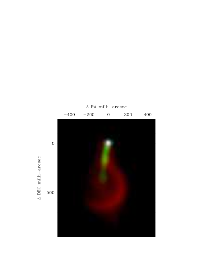
Figure 1: Keck Telescope laser adaptive-optics integral field spectroscopy image with OSIRIS by K. W. Hodapp of SVS 13 on 2011 August 21. The micro-jet is traced by the emission of the shock excited 1.644 $\mu$m [Fe II] line (green) and the bow shock bubble is traced in the lower excitation 2.122 $\mu$m H₂ 1–0 S(1) line (red). The white disk is the stellar source. The micro-jet plus bubble region is approximately $10^{10}$ km on each side.

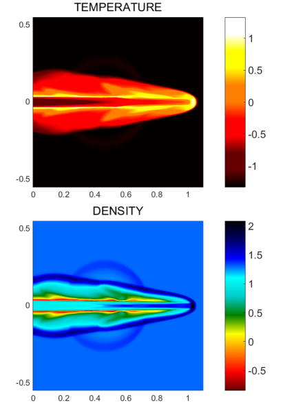
Figure 6: Cross section of the numerical simulation of the SVS 13 bow shock bubble and jet at 22.3 yr (circa 2012): logarithm of temperature $\log_{10}\left(T/\overline{T}\right)$, where $\overline{T}$ = $10^{4}$ K, and logarithm of density $\log_{10}\left(\rho/\overline{\rho}\right)$, where $\overline{\rho}$ = 100 H cm^-3. Lengths are in $10^{10}$ km.

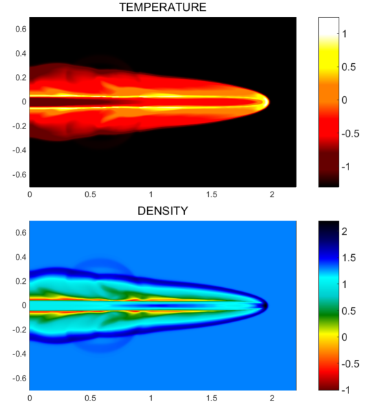
Figure 8: Cross section of the numerical simulation of the SVS 13 bow shock bubble and jet at 26.1 yr (circa 2016), assuming the jet source has not turned off: logarithm of temperature $\log_{10}\left(T/\overline{T}\right)$, where $\overline{T}$ = $10^{4}$ K, and logarithm of density $\log_{10}\left(\rho/\overline{\rho}\right)$, where $\overline{\rho}$ = 100 H cm^-3. Lengths are in $10^{10}$ km.