Observing quantum synchronization blockade in circuit quantum electrodynamics

Abstract

High quality factors, strong nonlinearities, and extensive design flexibility make superconducting circuits an ideal platform to investigate synchronization phenomena deep in the quantum regime. Recently [18], it was predicted that energy quantization and conservation can block the synchronization of two identical, weakly coupled nonlinear self-oscillators. Here we propose a Josephson junction circuit realization of such a system along with a simple homodyne measurement scheme to observe this effect. We also show that at finite detuning, where phase synchronization takes place, the two oscillators are entangled in the steady state as witnessed by the positivity of the logarithmic negativity.

1 Introduction

Synchronization of coupled self-sustained oscillating systems is a ubiquitous phenomenon in nature and appears in fields as diverse as biology [1, 2, 3], economics [4], sociology [5] and physics, where it was first scientifically described [6]. In the latter field an interesting question is what happens with synchronization in the quantum regime, i.e. when the limit cycle steady states of the oscillators are quantum states with no classical analog. Previous work on quantum synchronization has focused mainly on theoretically identifying and characterizing differences between classical and quantum synchronization [7, 8, 9, 10, 11, 12, 13, 14, 15, 16, 17, 18] and on potential applications of the latter [19, 20, 21]. Experimental observation of quantum synchronization phenomena is hindered by the stringent requirements of high quantum coherence and strong nonlinearities, both of which are also key requirements for quantum computation.

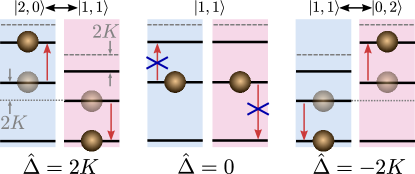
Figure 1: Energetics of quantum synchronization blockade of two weakly coupled anharmonic self-oscillators represented as three level systems with softening anharmonicity $2K$. A resonance between the states $\ket{1,1}$ and $\ket{2,0}$ ($\ket{0,2}$) requires a detuning $\hat{\Delta}=2K$ ($\hat{\Delta}=-2K$) between the oscillators.

Driven in large parts by the quest for a quantum computer, superconducting circuits realized with one or multiple Josephson junctions coupled to microwave resonators have become a versatile platform to study light-matter interaction at the single photon level. The design flexibility of superconducting circuits has enabled the realization of a wide range of Hamiltonians [22, 23, 24] and quantum reservoirs [25, 26, 27, 28] with great precision. This in turn has made possible the observation of textbook nonlinear quantum optics effects taking place in hitherto inaccessible regimes [22, 29].

Here we show that superconducting circuits form an ideal platform for studying synchronization of coupled nonlinear self-sustained oscillators deep in the quantum regime. In particular, we provide the blueprint of a circuit for observing the quantum synchronization blockade (QSB) recently predicted by Lörch et al. [18]: In contrast to the classical case where phase synchronization is maximal between two weakly interacting self-sustained oscillators of equal frequencies [30], phase synchronization between two weakly coupled nonlinear self-oscillators, individually stabilized to a Fock state, is suppressed on resonance. Intuition for this effect can be obtained in the perturbative limit of weak interactions [18] as illustrated in Fig. 1: To lowest order, a weak coupling between two nonlinear self-oscillators stabilized to the Fock state $\ket{1}$ can only lead to energy exchange when a finite detuning compensates for the anharmonicity. At zero detuning, energy conservation forbids the exchange of energy to leading order and synchronization is blocked.

At the heart synchronization is a form of correlation. In the quantum regime, the relation between synchronization and entanglement is of particular interest [8, 31, 11, 32]. This relation can also be used to define quantum synchronization: If the correlations present in the synchronized state are non-classical, i.e. if the two oscillators are in an entangled state, then synchronization is of quantum origin. Here we show that when synchronization occurs in our circuit, the steady state of the two oscillators is indeed entangled.

The focus here is on self-sustained nonlinear quantum oscillators, which are incoherently driven into non-classical steady states by a combination of nonlinear damping and amplification (anti-damping). Rips et al. [33] proposed a scheme to stabilize nonlinear nanomechanical oscillators into non-classical steady states by taking advantage of the quantized radiation pressure force between microwave photons and a nanomechanical oscillator.

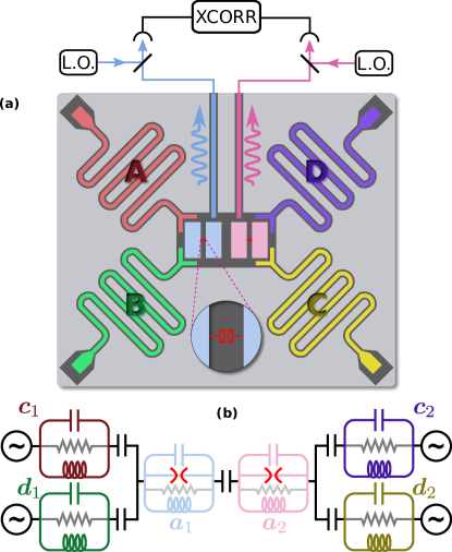
Figure 2: (a) Circuit layout of a coplanar waveguide (CPW) realization of the system. The upper part shows the measurement setup used to detect synchronization and its blockade in the homodyne cross-correlations. (b) Minimal lumped element circuit model (omitting the readout lines). Frequency multiplexing allows driving of all six modes via the four microwave ports shown.

Crucially, QSB can be observed only when the energy scale of the nonlinearity $K$ surpasses the damping rate $\kappa$ of the oscillator [18]. This single photon Kerr regime, where $\kappa\ll K$, has not yet been reached with nanomechanical oscillators currently precluding the observation of QSB in these systems. In contrast, owing to tremendous experimental progress [23], superconducting circuits have recently entered this regime [22] with ratios as large as $K/\kappa\simeq 10^{3}$. Thus motivated, we adapt the proposal of Rips et al. [33] to circuit quantum electrodynamics (cQED) replacing the nanomechanical oscillator with a transmon qubit. The major difficulty in doing so is that the natural (capacitive or inductive) interaction between superconducting oscillators is not of the radiation pressure form, which complicates engineering both nonlinear damping and amplification simultaneously. One of our key results is that we show that this can still be approximately achieved in the dispersive regime of cQED in a suitably displaced and rotated frame thus opening up the possibility to observe non-classical behavior of quantum synchronization with state-of-the-art superconducting circuits.

2 Circuit and model

A coplanar waveguide (CPW) realization of the superconducting circuit we consider is depicted in Fig. 2 (a) and consists of six oscillator circuits: Two capacitively coupled Josephson nonlinear oscillators at the center, each capacitively coupled to two linear microwave resonators. A minimal lumped element circuit model for the relevant modes (one mode per oscillator) is shown in Fig. 2 (b). The bare resonance frequencies of all six oscillators are detuned from each other by many times the coupling strengths. Hence, in this dispersive regime, where energy exchange is suppressed to first order, the normal modes of the linearized circuit remain close to the uncoupled modes and each oscillator can be associated with the corresponding normal mode as indicated by the color scheme of Fig. 2 (a) and (b). Interactions are generated by the two Josephson cosine nonlinearities (red spider symbols in Fig. 2 (b)), which couple the normal modes together [34, 35, 36, 37, 38]. Retaining only the dominant leading-order terms (see [39] for a full derivation), the unitary part of the dynamics of this quantum system is governed by the Hamiltonian $\bm{H}=\bm{H}_{\rm disp}+\bm{H}_{\rm control}$ with

$$\bm{H}_{\rm disp}=\sum_{j=1}^{2}\left(\Delta^{a}_{j}\bm{a}_{j}^{\dagger}\bm{a}_{j}+\Delta^{c}_{j}\bm{c}_{j}^{\dagger}\bm{c}_{j}+\Delta^{d}_{j}\bm{d}_{j}^{\dagger}\bm{d}_{j}-K_{j}\bm{a}_{j}^{\dagger}\bm{a}_{j}^{\dagger}\bm{a}_{j}\bm{a}_{j}-\raisebox{1.50696pt}{$\chi$}_{j}^{ac}\bm{a}_{j}^{\dagger}\bm{a}_{j}\bm{c}_{j}^{\dagger}\bm{c}_{j}-\raisebox{1.50696pt}{$\chi$}^{ad}_{j}\bm{a}_{j}^{\dagger}\bm{a}_{j}\bm{d}_{j}^{\dagger}\bm{d}_{j}\right)+J\bm{a}_{1}^{\dagger}\bm{a}_{1}\bm{a}_{2}^{\dagger}\bm{a}_{2},$$ (1)

$$\bm{H}_{\rm control}=\sum_{j=1}^{2}\left\{\varepsilon_{j}^{a}\left(\bm{a}_{j}+\bm{a}_{j}^{\dagger}\right)+\varepsilon_{j}^{c}\left(\bm{c}_{j}+\bm{c}_{j}^{\dagger}\right)+\varepsilon_{j}^{d}\left(\bm{d}_{j}+\bm{d}_{j}^{\dagger}\right)\right\}.$$ (2)

Here $\bm{a}_{i}$ is the bosonic annihilation operator of the normal mode associated with the nonlinear oscillator $i\in\{1,2\}$, which is coupled to two linear resonators with associated normal mode operators $\bm{c}_{i}$ and $\bm{d}_{i}$. This Hamiltonian is written in a frame rotating with the drives such that $\Delta^{a}_{j},\Delta^{c}_{j}$ and $\Delta^{d}_{j}$ denote the detunings between the corresponding resonators and drives. The rotating wave approximation (RWA) has been applied and the dominant interactions between the modes present in Eq. (1), which stem from the $\bm{\varphi}^{4}$ term of the Josephson potentials, are of self-Kerr ($K_{j}$) and cross-Kerr ($J$, $\raisebox{1.50696pt}{$\chi$}_{j}^{ac}$ and $\raisebox{1.50696pt}{$\chi$}_{j}^{ad}$) form.

The other crucial ingredient to achieve the desired limit cycle steady state is dissipation due to photon losses, which, in typical quantum optics fashion, is captured via the zero temperature Lindblad master equation

$$\bm{\dot{\rho}} =-i[\bm{H},\bm{\rho}]$$ (3)

$$+\sum_{i=1,2}\left(\kappa_{i}^{a}\mathcal{D}[\bm{a}_{i}]+\kappa_{i}^{c}\mathcal{D}[\bm{c}_{i}]+\kappa_{i}^{d}\mathcal{D}[\bm{d}_{i}]\right)\bm{\rho},$$

with dissipator $\mathcal{D}[\bm{O}]\bm{\rho}=\bm{O}\bm{\rho}\bm{O}^{\dagger}-\frac{1}{2}\{\bm{O}^{\dagger}\bm{O},\bm{\rho}\}$, where $\{\bm{A},\bm{B}\}=\bm{A}\bm{B}+\bm{B}\bm{A}$. Here $\kappa_{i}^{a}$ describes photon losses in the nonlinear oscillator $i$ and in Section 5 we will use this channel for measurements. The rates $\kappa_{i}^{c}$ and $\kappa_{i}^{d}$ account for photon losses in the linear resonators and we shall assume $\kappa_{i}^{a}\ll\kappa_{i}^{c},\kappa_{i}^{d}$, as motivated further below.

3 Fock state stabilization ($J=0$)

To enter the regime of quantum synchronization blockade the nonlinear self-oscillators need to be stabilized to a Fock state [18]. Fock state stabilization in linear superconducting oscillators has been achieved in [40] by means of an autonomous feedback mechanism mediated by a strong dispersive interaction with a qubit. Here we show that the system modeled by Eqs. (1–3), with $J=0$ can be used to stabilize a Fock state in the nonlinear oscillators. To do so we adapt the proposal of Rips et al. [33] for stabilizing a single phonon Fock state of a nonlinear nano-mechanical oscillator to the stabilization of a photonic Fock state of a nonlinear superconducting oscillator. Details of our derivation are provided in [39]. In the following we sketch the main steps focusing on the differences with [33].

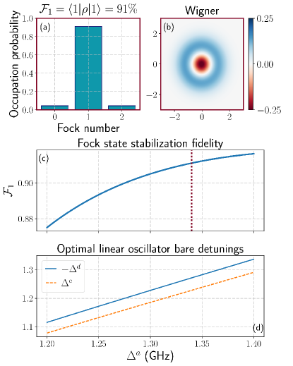
Figure 3: Fock state stabilization. (a) Photon number distribution of the nonlinear oscillator in the steady state. (b) Wigner function of the steady state. (c) Fidelity of the stabilized state to the Fock state $\ket{1}$ as a function of the nonlinear oscillator detuning. (d) Detunings of the linear oscillators for optimal stabilization. These results are obtained by numerically integrating the master equation (3) with $J=0$ and parameters $\kappa^{a}=100\,{\rm kHz}$, $\kappa^{c}=\kappa^{d}=10\,{\rm MHz}$, $K=30\,{\rm MHz}$, $\raisebox{1.50696pt}{$\chi$}^{ac}=\raisebox{1.50696pt}{$\chi$}^{ad}=8\,{\rm MHz}$, $\varepsilon^{a}=500\,{\rm MHz}$ and $\varepsilon^{c}=\varepsilon^{d}=2\,{\rm GHz}$.

Since $J=0$, we can concentrate on the subsystem consisting of oscillator modes $\bm{a}_{1}$, $\bm{c}_{1}$ and $\bm{d}_{1}$ without loss of generality and for compactness we drop the subscript $1$ in what follows. The central new idea here is to use the drive terms in $\bm{H}_{\rm control}$ to coherently displace the modes, i.e. $\bm{a}\rightarrow\bm{a}+\alpha$, $\bm{c}\rightarrow\bm{c}+\gamma$ and $\bm{d}\rightarrow\bm{d}+\delta$, such as to generate, via the cross-Kerr terms, a Rabi-type coupling between the linear and nonlinear oscillators:

$$\raisebox{1.50696pt}{$\chi$}^{ac}\bm{a}^{\dagger}\bm{a}\bm{c}^{\dagger}\bm{c} +\raisebox{1.50696pt}{$\chi$}^{ad}\bm{a}^{\dagger}\bm{a}\bm{d}^{\dagger}\bm{d}$$ (4)

$${\mathmakebox[\widthof{{}+{}}][c]{{\downarrow}}}$$

$$\raisebox{1.50696pt}{$\chi$}^{ac}\left(\alpha^{*}\bm{a}+\alpha\bm{a}^{\dagger}\right) \left(\gamma^{*}\bm{c}+\gamma\bm{c}^{\dagger}\right)+$$

$$\raisebox{1.50696pt}{$\chi$}^{ad}\left(\alpha^{*}\bm{a}+\alpha\bm{a}^{\dagger}\right) \left(\delta^{*}\bm{d}+\delta\bm{d}^{\dagger}\right)+\dots$$ (5)

The displacement amplitudes are given by $\alpha=-\varepsilon^{a}/(\Delta^{a}-i\kappa^{a}/2)$, $\gamma=-\varepsilon^{c}/(\Delta^{c}-i\kappa^{c}/2)$ and $\delta=-\varepsilon^{d}/(\Delta^{d}-i\kappa^{d}/2)$. These amplitudes are chosen such as to cancel the drive terms upon displacing the quadratic and dissipative terms. The displacement generates additional terms indicated by the ellipses in Eq. (5). The effect of most of these terms can be neglected in RWA, but some terms are non-rotating and lead to renormalizations of the oscillator frequencies: $\Delta^{a}\rightarrow\tilde{\Delta}^{a}=\Delta^{a}-\raisebox{1.50696pt}{$\chi$}^{ac}|\gamma|^{2}-\raisebox{1.50696pt}{$\chi$}^{ad}|\delta|^{2}$ and $\Delta^{c}\rightarrow\tilde{\Delta}^{c}=\Delta^{c}-\raisebox{1.50696pt}{$\chi$}^{ac}|\alpha|^{2}$ as well as $\Delta^{d}\rightarrow\tilde{\Delta}^{d}=\Delta^{d}-\raisebox{1.50696pt}{$\chi$}^{ad}|\alpha|^{2}$. In addition, the displacement transformation of the Kerr term of the $\bm{a}$ mode generates two more non-rotating terms: The first one leads to an additional frequency renormalization: $\tilde{\Delta}^{a}\rightarrow\hat{\Delta}^{a}=\tilde{\Delta}^{a}-4K|\alpha|^{2}$ and the second one is the squeezing term $K(\alpha^{*2}\bm{a}^{2}+\alpha^{2}\bm{a}^{\dagger 2})$. The latter can potentially adversely affect Fock state stabilization. However, we find that its effect on the steady state is negligible if the displacement amplitude $\alpha$ of the nonlinear oscillator remains small compared with the displacement amplitudes $\gamma$ and $\delta$ of the linear oscillators such that $K/\raisebox{1.50696pt}{$\chi$}^{ac}\ll|\gamma/\alpha|$ as well as $K/\raisebox{1.50696pt}{$\chi$}^{ad}\ll|\delta/\alpha|$.

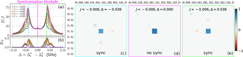
Figure 4: (a) Normalized quantum synchronization measure $S/J$ as a function of the bare detuning $\Delta=\Delta_{1}^{a}-\Delta_{2}^{a}$ between the two nonlinear self-oscillators for different values of the bare inter-oscillator dispersive coupling strength $J$. $\Delta_{2}^{a}$ is varied while $\Delta_{1}^{a}$ is kept fixed. The steady state is obtained from a quantum trajectory simulation by averaging the long time (i.e. $t\gg 1/\gamma_{\pm}$) temporal averages over $500$ trajectories. (b) Logarithmic negativity $E_{N}={\rm log_{2}}||\bm{\rho}_{\rm ss}^{\rm PT}||_{1}$, showing that when the oscillators synchronize, entanglement is present, i.e. $E_{N}>0$. (c) to (e) Hinton diagrams at three different values of $\Delta$ showing off-resonant synchronization (c) and (e) and synchronization blockade on resonance (d). The area of the squares is proportional to the amplitude of the complex number $\mathinner{\langle{k,l|\bm{\rho}_{\rm ss}|m,n}\rangle}$ in Fock space and the color corresponds to its real part. Correlations between the states $\ket{1,1}$ and $\ket{2,0}$ respectively $\ket{0,2}$ are clearly visible off resonance ((c) and (e)) but are absent on resonance (d). Animations over the full range of detunings are provided at this url [39]. Parameter values are the same as in Fig. 3.

Together with appropriately detuned drives, the interaction of Eq. (5), allows a state with a narrow excitation number distribution centered around $n_{0}\in\mathbb{N}$ to be stabilized. Specifically this requires that $\hat{\Delta}^{a}=\tilde{\Delta}^{c}+\Delta_{\downarrow}$ as well as $\hat{\Delta}^{a}=-\tilde{\Delta}^{d}+\Delta_{\uparrow}$, where $\Delta_{\downarrow}=2Kn_{0}\ll|\hat{\Delta}^{a}+\tilde{\Delta}^{c}|$ and $\Delta_{\uparrow}=2K(n_{0}-1)\ll|\hat{\Delta}^{a}-\tilde{\Delta}^{d}|$. Under these conditions, the red and blue sideband terms $\raisebox{1.50696pt}{$\chi$}^{ac}\alpha^{*}\gamma\bm{a}^{\dagger}\bm{c}+{\rm H.c.}$, and $\raisebox{1.50696pt}{$\chi$}^{ad}\alpha^{*}\delta^{*}\bm{a}\bm{d}+{\rm H.c.}$, are made simultaneously resonant, while the counter-rotating terms $\raisebox{1.50696pt}{$\chi$}_{ac}\alpha\gamma\bm{a}\bm{c}+{\rm H.c.}$ and $\raisebox{1.50696pt}{$\chi$}_{ad}\alpha\delta^{*}\bm{a}^{\dagger}\bm{d}+{\rm H.c.}$ can be neglected in RWA. When $|\alpha\gamma\raisebox{1.50696pt}{$\chi$}^{ac}|,|\alpha\delta\raisebox{1.50696pt}{$\chi$}^{ad}|\ll\kappa^{c},\kappa^{d}$, the modes of the linear oscillators can further be adiabatically eliminated yielding an effective master equation with a Lorentzian spectrum for a Kerr oscillator with nonlinear damping and amplification [39, 33, 18]:

$$\bm{\dot{\rho}} =-i[\bm{H}_{K},\bm{\rho}]+\kappa^{a}\mathcal{D}\left[\bm{a}\right]\bm{\rho}$$ (6)

$$+\gamma_{\uparrow}\sum_{m}L_{m}\mathcal{D}\left[\sqrt{m}\ket{m}\bra{m-1}\right]\bm{\rho}$$

$$+\gamma_{\downarrow}\sum_{m}L_{m}\mathcal{D}\left[\sqrt{m+1}\ket{m}\bra{m+1}\right]\bm{\rho}.$$

Here $\gamma_{\uparrow}=4|\alpha\delta\raisebox{1.50696pt}{$\chi$}^{ad}|^{2}/\kappa$, $\gamma_{\downarrow}=4|\alpha\gamma\raisebox{1.50696pt}{$\chi$}^{ac}|^{2}/\kappa$, $L_{m}=\sigma^{2}/[(n_{0}-m)^{2}+\sigma^{2}]$, $\sigma=\kappa/(4K)$ and $\bm{H}_{K}=\hat{\Delta}^{a}\bm{a}^{\dagger}\bm{a}-K\bm{a}^{\dagger}\bm{a}^{\dagger}\bm{a}\bm{a}$. For compactness we consider the case where $\kappa^{c}=\kappa^{d}=\kappa$. When $\kappa\ll 2K$, the dominant transitions are $n_{0}-1\rightarrow n_{0}$ at rate $\gamma_{\uparrow}L_{n_{0}}$ and $n_{0}+1\rightarrow n_{0}$ at rate $\gamma_{\downarrow}L_{n_{0}}$. The system is thus stabilized in the Fock state $\ket{n_{0}}$, which is an eigenstate of $\bm{H}_{K}$.

Fig. 3 shows the results of a numerical simulation with the full model with $J=0$ (Eqs. (1–3)), which includes all the counter-rotating terms. Because of the frequency renormalization, we cannot directly obtain the values of the bare detunings. Instead, for each value of $\Delta^{a}$ we determine the corresponding values of $\Delta^{c}$ and $\Delta^{d}$ by maximizing the fidelities to the target Fock state (Fig. 3 (d)). The achievable fidelities (Fig. 3 (c)) range roughly between $88\%$ and $92\%$ and increase with increasing detuning of the drive oscillators consistent with the RWA. Thus we have established that the Fock state stabilizing dynamics of Eq. (6) can be engineered in our circuit. We next turn to the case of two coupled systems, i.e. $J\not=0$.

4 Quantum synchronization blockade

Classically, two weakly coupled self-oscillators display phase synchronization, i.e. the relative phase between the two oscillators is narrowly distributed around a fixed value in the steady state [30]. This synchronization is strongest on resonance, i.e. when the two isolated systems oscillate at the same frequency. In contrast, Lörch et al. [18] predict that if two identical Fock state stabilized Kerr oscillators are weakly coupled with each other by a linear term of the form $J(\bm{a}_{1}^{\dagger}\bm{a}_{2}+{\rm H.c.})$, phase synchronization is suppressed at zero detuning in stark contrast to the classical situation.

In our system (Eqs. (1) and (2)), a linear coupling is obtained naturally in the displaced frame when $J\not=0$, since $J\bm{a}_{1}^{\dagger}\bm{a}_{1}\bm{a}_{2}^{\dagger}\bm{a}_{2}\rightarrow J\left(\alpha_{1}\alpha_{2}^{*}\bm{a}_{1}^{\dagger}\bm{a}_{2}+\alpha_{1}^{*}\alpha_{2}\bm{a}_{2}^{\dagger}\bm{a}_{1}\right)+\dots$, where the ellipses denote additional terms. Among the latter the only relevant ones under RWA are $J|\alpha_{1}|^{2}\bm{a}_{2}^{\dagger}\bm{a}_{2}$ and $J|\alpha_{2}|^{2}\bm{a}_{1}^{\dagger}\bm{a}_{1}$, which lead to an additional frequency renormalization.

To quantify phase synchronization we follow [41, 18] and use the measure

$$S=2\pi\,\underset{\phi}{\rm max}\left[P(\phi)\right]-1,$$ (7)

with $P(\phi)=\int_{0}^{2\pi}d\phi_{1}d\phi_{2}\delta(\phi_{1}-\phi_{2}-\phi)p(\phi_{1},\phi_{2})$ and $p(\phi_{1},\phi_{2})=\mathinner{\langle{\phi_{1},\phi_{2}|\bm{\rho}_{\rm ss}|\phi_{1},\phi_{2}}\rangle}$ and $\ket{\phi_{i}}=(2\pi)^{-1}\sum_{n=0}^{\infty}e^{in\phi_{i}}\ket{n}$. Here $\bm{\rho}_{\rm ss}$ denotes the steady state reduced density matrix of the two nonlinear oscillators. The quantity $S\geq 0$ essentially measures how

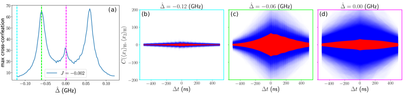
Figure 5: (a) Maximum of the averaged cross-correlated homodyne signals as a function of the renormalized detuning $\hat{\Delta}$ between the nonlinear oscillators. Clearly the cross-correlation mirrors the synchronization measure of Fig. 4 (a). (b) to (d) Cross-correlation functions of the homodyne signals corresponding to the three different values of $\hat{\Delta}$ marked by dashed vertical lines in (a). The individual trajectories are shown in blue and the average over $1000$ trajectories is shown in red. Parameter values are the same as in Figs. 3 and 4.

uniform the relative phase distribution of the two oscillators is. In the absence of synchronization $S=0$ and the larger $S$ is, the stronger the synchronization. Fig. 4 confirms that quantum synchronization blockade does indeed occur in our system as reflected by a suppression of $S$ on resonance (Fig. 4 (a)). At finite detuning, when the resonance condition $\hat{\Delta}\equiv\hat{\Delta}_{1}^{a}-\hat{\Delta}_{2}^{a}=\pm 2K$ is satisfied, the phases of the oscillators synchronize as indicated by the presence of peaks in $S$ (Fig. 4 (a)). Notice that the spacing between the two major peaks is reduced compared with the ideal separation of $4K$. This is due to the frequency renormalization $\Delta\rightarrow\hat{\Delta}$ discussed above and to the coupling, which split the resonances by $\pm J$. As the coupling strength $J$ increases, off-resonant synchronization is reduced and a small bump appears on resonance. Also, because the fidelity of Fock state stabilization (for $J=0$) depends on the detuning (Fig. 3 (c)), the synchronization signal is slightly stronger for positive than for negative detunings.

Interestingly, when the two oscillators synchronize, their state is entangled as witnessed by the positivity of the logarithmic negativity [42] $E_{N}={\rm log_{2}}||\bm{\rho}_{\rm ss}^{\rm PT}||_{1}$ (Fig. 4 (b)). Here $\bm{\rho}_{\rm ss}^{\rm PT}$ denotes the steady state density matrix partially transposed with respect to one of the two oscillators and $||\bm{\rho}||_{1}={\rm tr}\sqrt{\bm{\rho}\bm{\rho}^{\dagger}}$ is the trace norm. To gain further insight into the nature of the blocked and the synchronized states we plot Hinton diagrams of $\bm{\rho}_{\rm ss}$ for $J=-6\,{\rm MHz}$ for the resonant case $\Delta=0$ (Fig. 4 (d)) and for the two bare detunings $\Delta\simeq\pm 0.036\,{\rm GHz}$, which correspond to a synchronization resonance (Fig. 4 (c) and (e)). When $\Delta=0$, the two oscillators are essentially in the tensor product state $\ket{1,1}$. For $\Delta=-0.036\,{\rm GHz}$ ($\Delta=0.036\,{\rm GHz}$) this state hybridizes with the state $\ket{0,2}$ ($\ket{2,0}$) resulting ideally in the entangled doublet $c_{11}\ket{1,1}\pm c_{02}\ket{0,2}$ ($c_{11}\ket{1,1}\pm c_{20}\ket{2,0}$). The amplitudes $c_{11}$, $c_{20}$ and $c_{02}$ are determined by the competition between the localizing Fock state stabilization and the delocalizing inter-oscillator coupling. Since here the coupling is weak the former dominates leading to a relatively small by-mixing of the states $\ket{2,0}$ and $\ket{0,2}$. Animations illustrating the synchronization blockade and the splitting of the resonances as $\Delta$ is varied can be found at this url [39].

5 Homodyne detection of quantum synchronization and its blockade

While the synchronization measure $S$ is convenient for theoretical characterization, it can be challenging to measure since it requires full state tomography of the two nonlinear oscillators. Here we show that quantum synchronization and its blockade can be detected more simply by correlating the classical signals obtained from separate homodyne measurements of the phases of the nonlinear oscillators.

We choose the phases of the local oscillators such as to measure the $\bm{X}_{i}=\bm{a}_{i}+\bm{a}_{i}^{\dagger}$ quadratures. The homodyne signals from the two oscillators are then given by [43]

$$J_{i}(t)=\kappa_{i}^{a}\mathinner{\langle{\bm{X}_{i}}\rangle}_{\rm H}+\sqrt{\kappa_{i}^{a}}\xi_{i}(t),$$ (8)

where $\xi_{i}(t)$ is a zero mean Gaussian white noise random process with unit variance and the subscript ${\rm H}$ indicates that the expectation value is conditioned on the particular quantum trajectory $\bm{\rho}_{\rm H}(t)$. The latter is a solution of the stochastic master equation

$$\bm{\dot{\rho}}_{\rm H} =\mathcal{\bm{L}}_{K}\bm{\rho}_{\rm H}+\sum_{i=1,2}\left(J_{i}-\kappa_{i}^{a}\mathinner{\langle{\bm{X}_{i}}\rangle}_{\rm H}\right)\mathcal{H}[\bm{a}_{i}]\bm{\rho}_{\rm H}.$$ (9)

Here $\mathcal{\bm{L}}_{K}$ is the Liouvillian superopertor generating the right-hand side of Eq. (6), $\kappa_{i}^{a}$ plays the role of the coupling to measurement device and $\mathcal{H}[\bm{O}]\bm{\rho}=\bm{O}\bm{\rho}+\bm{\rho}\bm{O}^{\dagger}-{\rm tr}[\bm{O}\bm{\rho}+\bm{\rho}\bm{O}^{\dagger}]\bm{\rho}$, describes the back-action of the homodyne measurement. The phase correlation between the two oscillators is reflected in the averaged cross-correlation of the measurement signals. Specifically we look at the maximum of the averaged cross-correlation given by

$$\mathbb{E}\left[C_{\tau}(J_{1},J_{2})\right]=(\kappa_{1}^{a}\kappa_{2}^{a})\mathbb{E}\left[C_{\tau}(\mathinner{\langle{X_{1}}\rangle}_{\rm H},\mathinner{\langle{X_{2}}\rangle}_{\rm H})\right],$$ (10)

where $C_{\tau}(x,y)=\int_{0}^{T}x(t)y(t-\tau)dt$ is the cross-correlation function, $T\gg\gamma_{\uparrow}^{-1},\gamma_{\downarrow}^{-1}$ is the measurement time, and $\mathbb{E}[\cdot]$ denotes the average value over trajectories. Fig. 5 shows the results of a stochastic master equation simulation using the effective model (6) for each oscillator with the same parameter values as used in Figs. 3 and 4. This confirms that phase synchronization and its blockade as quantified by $S$ (Eq. (7)), are indeed reflected in the cross-correlations of the homodyne signals. It is worthwhile to emphasize the simplicity of this detection scheme and we hope that its adoption will accelerate progress on the experimental front.

6 Conclusions

Bath engineering with state-of-the-art superconducting circuits together with measurement methods typically used for quantum information processing offer a versatile approach to investigate quantum synchronization phenomena. We proposed and analyzed a circuit to test the recently predicted phenomenon of quantum synchronization blockade [18]. Its realization should be within reach of current technology. We also showed that off-resonant quantum synchronization in this system is accompanied by entanglement. Furthermore, we showed that quantum synchronization and its blockade can be detected in cross-correlations of homodyne signals, greatly simplifying their experimental identification. It is expected that the results presented here will also be relevant in the near future when it becomes possible to build larger networks of high-Q nonlinear superconducting oscillators. Such systems are predicted to display a rich variety of quantum effects [44, 18] and have potential technological applications [19, 45, 46, 47].

Acknowledgments: This work was supported by the Swiss National Science Foundation (SNSF) and the NCCR QSIT. We acknowledge interesting discussions with Niels Lörch, Andreas Nunnenkamp, Rakesh Tiwari and Christoph Bruder. The numerical computations were peformed in a parallel computing environment at sciCORE (http://scicore.unibas.ch/) scientific computing core facility at University of Basel using the Python libraries NumPy (http://www.numpy.org/) and QuTip (http://qutip.org/). The graphics were created with Matplotlib (http://www.matplotlib.org).

References

- Strogatz and Stewart [1993] S. H. Strogatz and I. Stewart, Scientific American 269, 102 (1993).
- Glass [2001] L. Glass, Nature 410, 277 (2001), ISSN 0028-0836, URL http://dx.doi.org/10.1038/35065745.
- Chen et al. [2017] C. Chen, S. Liu, X.-q. Shi, H. Chaté, and Y. Wu, Nature 542, 210 (2017), ISSN 0028-0836, letter, URL http://dx.doi.org/10.1038/nature20817.
- Krause et al. [2015] S. M. Krause, S. Börries, and S. Bornholdt, Phys. Rev. E 92, 012815 (2015), URL https://link.aps.org/doi/10.1103/PhysRevE.92.012815.
- Bloch et al. [2013] G. Bloch, E. D. Herzog, J. D. Levine, and W. J. Schwartz, Proceedings of the Royal Society of London B: Biological Sciences 280 (2013), ISSN 0962-8452, http://rspb.royalsocietypublishing.org/content/280/1765/20130035.full.pdf, URL http://rspb.royalsocietypublishing.org/content/280/1765/20130035.
- Hugenii [1673] C. Hugenii, Horoloquim Oscilatorium (1673), english translation, The Pendulum Clock (Iowa State University Press, Ames, Iowa, 1986).
- Zhirov, O. V. and Shepelyansky, D. L. [2006] Zhirov, O. V. and Shepelyansky, D. L., Eur. Phys. J. D 38, 375 (2006), URL https://doi.org/10.1140/epjd/e2006-00011-9.
- Zhirov and Shepelyansky [2009] O. V. Zhirov and D. L. Shepelyansky, Phys. Rev. B 80, 014519 (2009), URL https://link.aps.org/doi/10.1103/PhysRevB.80.014519.
- Mari et al. [2013] A. Mari, A. Farace, N. Didier, V. Giovannetti, and R. Fazio, Phys. Rev. Lett. 111, 103605 (2013), URL https://link.aps.org/doi/10.1103/PhysRevLett.111.103605.
- Lee and Sadeghpour [2013] T. E. Lee and H. R. Sadeghpour, Phys. Rev. Lett. 111, 234101 (2013), URL https://link.aps.org/doi/10.1103/PhysRevLett.111.234101.
- Lee et al. [2014] T. E. Lee, C.-K. Chan, and S. Wang, Phys. Rev. E 89, 022913 (2014), URL https://link.aps.org/doi/10.1103/PhysRevE.89.022913.
- Walter et al. [2014] S. Walter, A. Nunnenkamp, and C. Bruder, Phys. Rev. Lett. 112, 094102 (2014), URL https://link.aps.org/doi/10.1103/PhysRevLett.112.094102.
- Walter et al. [2015] S. Walter, A. Nunnenkamp, and C. Bruder, Annalen der Physik 527, 131 (2015), ISSN 1521-3889, URL http://dx.doi.org/10.1002/andp.201400144.
- Ameri et al. [2015] V. Ameri, M. Eghbali-Arani, A. Mari, A. Farace, F. Kheirandish, V. Giovannetti, and R. Fazio, Phys. Rev. A 91, 012301 (2015), URL https://link.aps.org/doi/10.1103/PhysRevA.91.012301.
- Weiss et al. [2016] T. Weiss, A. Kronwald, and F. Marquardt, New Journal of Physics 18, 013043 (2016), URL http://stacks.iop.org/1367-2630/18/i=1/a=013043.
- Fiderer et al. [2016] L. J. Fiderer, M. Kuś, and D. Braun, Phys. Rev. A 94, 032336 (2016), URL https://link.aps.org/doi/10.1103/PhysRevA.94.032336.
- Lörch et al. [2016] N. Lörch, E. Amitai, A. Nunnenkamp, and C. Bruder, Phys. Rev. Lett. 117, 073601 (2016), URL https://link.aps.org/doi/10.1103/PhysRevLett.117.073601.
- Lörch et al. [2017] N. Lörch, S. E. Nigg, A. Nunnenkamp, R. P. Tiwari, and C. Bruder, Phys. Rev. Lett. 118, 243602 (2017), URL https://link.aps.org/doi/10.1103/PhysRevLett.118.243602.
- Makino et al. [2016] K. Makino, Y. Hashimoto, J.-i. Yoshikawa, H. Ohdan, T. Toyama, P. van Loock, and A. Furusawa, Science Advances 2 (2016), http://advances.sciencemag.org/content/2/5/e1501772.full.pdf, URL http://advances.sciencemag.org/content/2/5/e1501772.
- Giorgi et al. [2016] G. L. Giorgi, F. Galve, and R. Zambrini, Phys. Rev. A 94, 052121 (2016), URL https://link.aps.org/doi/10.1103/PhysRevA.94.052121.
- Bellomo et al. [2017] B. Bellomo, G. L. Giorgi, G. M. Palma, and R. Zambrini, Phys. Rev. A 95, 043807 (2017), URL https://link.aps.org/doi/10.1103/PhysRevA.95.043807.
- Kirchmair et al. [2013] G. Kirchmair, B. Vlastakis, Z. Leghtas, S. E. Nigg, H. Paik, E. Ginossar, M. Mirrahimi, L. Frunzio, S. M. Girvin, and R. J. Schoelkopf, Nature 495, 205 (2013).
- Devoret and Schoelkopf [2013] M. H. Devoret and R. J. Schoelkopf, Science 339, 1169 (2013), ISSN 0036-8075, http://science.sciencemag.org/content/339/6124/1169.full.pdf, URL http://science.sciencemag.org/content/339/6124/1169.
- Anderson et al. [2016] B. M. Anderson, R. Ma, C. Owens, D. I. Schuster, and J. Simon, Phys. Rev. X 6, 041043 (2016), URL https://link.aps.org/doi/10.1103/PhysRevX.6.041043.
- Shankar et al. [2013] S. Shankar, M. Hatridge, Z. Leghtas, K. M. Sliwa, A. Narla, U. Vool, S. M. Girvin, L. Frunzio, M. Mirrahimi, and M. H. Devoret, Nature 504, 419 (2013), ISSN 0028-0836, letter, URL http://dx.doi.org/10.1038/nature12802.
- Kimchi-Schwartz et al. [2016] M. E. Kimchi-Schwartz, L. Martin, E. Flurin, C. Aron, M. Kulkarni, H. E. Tureci, and I. Siddiqi, Phys. Rev. Lett. 116, 240503 (2016), URL https://link.aps.org/doi/10.1103/PhysRevLett.116.240503.
- Liu et al. [2016] Y. Liu, S. Shankar, N. Ofek, M. Hatridge, A. Narla, K. M. Sliwa, L. Frunzio, R. J. Schoelkopf, and M. H. Devoret, Phys. Rev. X 6, 011022 (2016), URL https://link.aps.org/doi/10.1103/PhysRevX.6.011022.
- Albert et al. [2016] V. V. Albert, B. Bradlyn, M. Fraas, and L. Jiang, Phys. Rev. X 6, 041031 (2016), URL https://link.aps.org/doi/10.1103/PhysRevX.6.041031.
- Toyli et al. [2016] D. M. Toyli, A. W. Eddins, S. Boutin, S. Puri, D. Hover, V. Bolkhovsky, W. D. Oliver, A. Blais, and I. Siddiqi, Phys. Rev. X 6, 031004 (2016), URL https://link.aps.org/doi/10.1103/PhysRevX.6.031004.
- Pikovsky et al. [2003] A. Pikovsky, M. Rosenblum, and J. Kurths, Synchronization: A Universal Concept in Nonlinear Sciences (Cambridge University Press, 2003).
- Manzano et al. [2013] G. Manzano, F. Galve, G. L. Giorgi, E. Hernandez-Garcia, and R. Zambrini, Scientific Reports 3, 1439 EP (2013), article, URL http://dx.doi.org/10.1038/srep01439.
- Witthaut et al. [2017] D. Witthaut, S. Wimberger, R. Burioni, and M. Timme, Nature Communications 8, 14829 EP (2017), article, URL http://dx.doi.org/10.1038/ncomms14829.
- Rips et al. [2012] S. Rips, M. Kiffner, I. Wilson-Rae, and M. J. Hartmann, New Journal of Physics 14, 023042 (2012), URL http://stacks.iop.org/1367-2630/14/i=2/a=023042.
- Nigg et al. [2012] S. E. Nigg, H. Paik, B. Vlastakis, G. Kirchmair, S. Shankar, L. Frunzio, M. H. Devoret, R. J. Schoelkopf, and S. M. Girvin, Phys. Rev. Lett. 108, 240502 (2012), URL http://link.aps.org/doi/10.1103/PhysRevLett.108.240502.
- Bourassa et al. [2012] J. Bourassa, F. Beaudoin, J. M. Gambetta, and A. Blais, Phys. Rev. A 86, 013814 (2012), URL http://link.aps.org/doi/10.1103/PhysRevA.86.013814.
- Solgun et al. [2014] F. Solgun, D. W. Abraham, and D. P. DiVincenzo, Phys. Rev. B 90, 134504 (2014), URL https://link.aps.org/doi/10.1103/PhysRevB.90.134504.
- Smith et al. [2016] W. C. Smith, A. Kou, U. Vool, I. M. Pop, L. Frunzio, R. J. Schoelkopf, and M. H. Devoret, Phys. Rev. B 94, 144507 (2016), URL https://link.aps.org/doi/10.1103/PhysRevB.94.144507.
- Malekakhlagh et al. [2016] M. Malekakhlagh, A. Petrescu, and H. E. Türeci, Phys. Rev. A 94, 063848 (2016), URL https://link.aps.org/doi/10.1103/PhysRevA.94.063848.
- [39] See ancillary files on the arxiv abstract page of the article.
- Holland et al. [2015] E. T. Holland, B. Vlastakis, R. W. Heeres, M. J. Reagor, U. Vool, Z. Leghtas, L. Frunzio, G. Kirchmair, M. H. Devoret, M. Mirrahimi, et al., Phys. Rev. Lett. 115, 180501 (2015), URL https://link.aps.org/doi/10.1103/PhysRevLett.115.180501.
- Hush et al. [2015] M. R. Hush, W. Li, S. Genway, I. Lesanovsky, and A. D. Armour, Phys. Rev. A 91, 061401 (2015), URL https://link.aps.org/doi/10.1103/PhysRevA.91.061401.
- Plenio [2005] M. B. Plenio, Phys. Rev. Lett. 95, 090503 (2005), URL https://link.aps.org/doi/10.1103/PhysRevLett.95.090503.
- Wiseman and Milburn [2009] H. M. Wiseman and G. J. Milburn, Quantum Measurement and Control (Cambridge Univ. Press, 2009).
- Benedetti et al. [2016] C. Benedetti, F. Galve, A. Mandarino, M. G. A. Paris, and R. Zambrini, Phys. Rev. A 94, 052118 (2016), URL https://link.aps.org/doi/10.1103/PhysRevA.94.052118.
- Li et al. [2017] W. Li, C. Li, and H. Song, Phys. Rev. E 95, 022204 (2017), URL https://link.aps.org/doi/10.1103/PhysRevE.95.022204.
- Nigg et al. [2017] S. E. Nigg, N. Lörch, and R. P. Tiwari, Science Advances 3 (2017), http://advances.sciencemag.org/content/3/4/e1602273.full.pdf, URL http://advances.sciencemag.org/content/3/4/e1602273.
- Puri et al. [2017] S. Puri, C. K. Andersen, A. L. Grimsmo, and A. Blais, 8, 15785 EP (2017), article, URL http://dx.doi.org/10.1038/ncomms15785.