Plus-Minus Player Ratings for Soccer

Abstract

The paper presents a plus-minus rating for use in association football (soccer). We first describe the standard plus-minus methodology as used in basketball and ice-hockey and then adapt it for use in soccer. The usual goal-differential plus-minus is considered before two variations are proposed. For the first variation, we present a methodology to calculate an expected goals plus-minus rating. The second variation makes use of in-play probabilities of match outcome to evaluate an expected points plus-minus rating. We use the ratings to examine who are the best players in European football, and demonstrate how the players’ ratings evolve over time. Finally, we shed light on the debate regarding which is the strongest league. The model suggests the English Premier League is the strongest, with the German Bundesliga a close runner-up.

1 Introduction

In sport, there is great interest in evaluating and measuring the performance of players. In team sports, owners, managers and coaches want to identify which players are key to their team’s success, so that recruitment and retention of players can be properly informed. Unlike other industries, there is much external interest in the performance of a sports team’s employees from, for example, fans and the media wanting to know which players to support, and which to berate. As such, one of the main tasks of sports analytics is to evaluate the performance of players and understand their contribution to the team’s results.

In this paper we present two modifications of the well-known plus-minus (PM) ratings model previously used to identify key players in basketball (see, for example, Sill, (2010)) and ice-hockey (see, for example, Macdonald, 2012a ). The PM ratings system is simple and intuitive, and provides an answer to the question: ‘how does a team perform with a player, compared to without the player?’. The modifications we propose are specific to soccer - a game in which it is notoriously difficult to rate players objectively.

For individual sports like tennis and chess, rating players is perhaps simpler than for team sports. Paired comparisons models are well-established and several variations exist. McHale and Morton, (2011) provide a ratings system for tennis for example. A perhaps more complex task is to estimate time-varying ratings for individuals which update following new information (the latest results). Elo ratings have been used for over half a century for rating chess players. Similarly, the Glicko rating system (Glickman,, 2012) provides a more theoretically justified model for estimating time-varying ratings of individuals.

More recently, attention has moved to using machine learning techniques to estimate player ratings. The TrueSkill rating (Herbrich et al.,, 2007) developed at Microsoft is a generalisation of the Elo ratings and is used for rating video game players.

Rating players in sports teams is more problematic. Players often have different responsibilities with some concentrated on offence (i.e. aiding scoring), whilst others are specialised in defence (i.e. helping to prevent scores for the opposition). A commonly used approach is to assign a value to a set of actions considered to be ‘of interest’ and to reward the player taking them with the associated value. This method was used for example in the EA SPORTS Player Performance Indicator (McHale et al.,, 2012) and is still used by the English Premier League as the official player ratings system. Due to its additivity, the previous approach provides simple, user-friendly player ratings and rankings. However, a cost of the simplicity is the lack of context and a deeper understanding of the situations in which actions were committed. Further, the data requirement is not trivial.

Models have been used to rate players for specific tasks. For example, Sáez Castillo et al., (2013) and McHale and Szczepański, (2014) present methods to identify the scoring ability of footballers whereas López Peña and Touchette, (2012), López Peña and Sánchez Navarro, (2015), Brooks et al., (2016) and Szczepański and McHale, (2016) deal with the passing aspect. But identifying the overall contribution of a player to a team’s success (or lack of it) has proven difficult in soccer. However, the concept of the PM ratings provides hope.

The concept of the PM rating is fundamentally different to the rating mechanisms discussed above. It directly measures the contribution a player has on a team’s success as measured by (the differential) of a target metric (goals for example). It does not make use of event data, and is not concerned with the number of actions a player might have achieved. All that matters is “whilst the player was on the pitch, what happened to the target metric?”.

The PM rating has been used extensively in ice-hockey (Macdonald, 2012a ; Spagnola, (2013)) and basketball (Sill, (2010); Fearnhead et al., (2011)). Indeed, PM ratings are now part of the statistics reported by the media (ESPN for example) and professional leagues (since 1968 the NHL has kept track of each player’s PM rating) in US team sports. Surprisingly, plus-minus ratings have yet to be adopted in soccer and are only discussed in some specialised forums but, to the best of our knowledge, have never been studied in the academic literature.

In this paper we propose to fill in the gap and adapt the plus-minus rating for use in soccer. We present the model currently used in basketball, and reported by ESPN before suggesting modifications to adapt the methodology for use in soccer. We then propose two extensions of the methodology using new target metrics measuring team success: first, we present an expected goals (xG) plus-minus rating (xGPM); and second, we present an expected Points (xP) plus-minus rating (xPPM). For the xGPM ratings we use a model to calculate the probability of a shot resulting in a goal. For the xPPM ratings we use an ‘in-play’ model to estimate the probability of each match outcome (win, draw, loss) given the current game state at any moment during the game. Both models are presented below.

The remainder of the paper is structured as follows: First, we describe the data used for this research (Section 1). In Section 3 we present the basic plus-minus rating and the regularized adjusted plus-minus rating currently used in basketball. In Section 4 we describe two new variations of the plus-minus ratings: an expected goals rating (xGPM), and an expected points plus-minus rating (xPPM). In Section 5 we use the ratings to look for the top players across European soccer, and see how their ratings evolve over time, before using the model to examine the relative strengths of European leagues. We conclude with some closing remarks in Section 6.

2 Data

We collected data from 11 European leagues over the last 8 seasons as detailed in Table 1. For every game in our data set, we collect the match date, the starting line-ups, timings of any goals, and timings and player names of any substitutions and red cards.

League	Seasons	Games
England Premier League	2009/10–2016/17	3,040
Germany Bundesliga I	2009/10–2016/17	2,448
Spain La Liga	2009/10–2016/17	3,039
Italy Serie A	2009/10–2016/17	3,037
Germany Bundesliga II	2015/16–2016/17	612
England Championship	2013/14–2016/17	2,227
Netherlands Eredivisie	2013/14–2016/17	1,242
Turkey Super Lig	2014/15–2016/17	918
Portugal Liga NOS	2016/17	306
France Ligue 1	2009/10–2016/17	3,039
Russia Premier League	2013/14–2016/17	960
Total		20,868

Table 1: Description of data used by league and season.

For the expected goals model developed in Section 4.1, additional information regarding shots is needed. Specifically, the shot time, the shooter $(x,y)$ coordinates, the type of shot (penalty, free-kick, header or open play), and the subjective “big chance” qualifier describing the shot situation are extracted from Opta F24 feed. On top of that, goal-keeper skills as reported by EA SPORTS FIFA video games are collected. They describe the keeper’s diving, ball handling, ball kicking, positioning, and reflexes skills. Mapping players between the Opta feed and EA SPORTS is done using the Google research tools to match players’ names and using the date of birth and the player’s country of birth for validation. Players not found by this method are mapped manually.

3 The Plus-Minus Rating

The plus-minus statistic has been in use since the 1950s in ice-hockey but is most seen nowadays applied to basketball. Indeed, the complexity of the game of basketball has led to several developments of the original concept. In this section we will first describe the basic plus-minus statistic, before presenting modifications that have been introduced in the literature. In what follows we will define everything in terms of soccer.

3.1 The Basic Plus-Minus Statistic

In its simplest form, a player’s plus-minus statistic can be used to answer the question: “what happens when the player is on the pitch, compared to when he is off it?”. Historically, goals (or points in basket ball) have been the preferred way to measure “what happened” and the raw plus-minus score calculates the player’s contribution to the goal difference of his team (per ninety minutes) whilst he is on the pitch. For example, consider a player who makes two match appearances. In the first match, he plays the first 60 minutes during which the team concedes one goal and fails to score itself. The match finishes in a 1-0 loss. In the second match, the player comes to the field with 30 minutes remaining and his team is enjoying being 3-0 ahead. During the 30 minutes of play he is on the pitch, the score moves to 5-0. The player’s plus-minus rating is then $((-1/60)+(2/30))\times 90=+4.5$. In other words, when the player was on the pitch the team scored 4.5 goals per 90 minutes more than the opposition.

The net plus-minus statistic can be used to measure the importance of a player to his team. This is simply the plus-minus statistic when the player is on the pitch minus the plus-minus statistic when the player is not on the pitch. In our example, the plus-minus statistic without the player is $((0/30)+(3/60))\times 90=4.5$, so that the net plus-minus statistic is 0. It appears then that the team is equally successful with and without the player.

This is of course a very simplistic picture and several pieces of information are not taken into account. For example, the effects of strengths of the other players on the pitch or of the game situation (such as a reduction in the number of players on a team following a red card, or of any home advantage) have not been accounted for. Further, if one was to use this simple plus-minus rating to compare players from different teams, the results would be almost meaningless. Consider two different players: one playing for the league champions and the other playing for the leagues worst team. Suppose both players had pure plus-minus ratings of 0. Who is likely the better player? Most sports fans would say that the player achieving a pure plus-minus of 0 on the league’s worst team probably deserves more credit in this example.

To account for these factors, the adjusted plus-minus statistic was introduced, and is described next.

3.2 Regularized Adjusted Plus-Minus

The adjusted plus-minus player metric was first described in Rosenbaum, (2004) who presented the plus-minus statistic as a regression problem. Doing so means ‘adjustments’ can be made to the basic plus-minus statistic to account for the strengths of the other players on a team, and of the opposition players. The set up is again simple. Define a segment of play to be one where the same set of players (usually two sides of 11 players) are on the pitch. A new segment is defined every time a new set of players are on the pitch. This may occur when a substitution is made, or when a sending off occurs, or for a different match. Each segment $t=1,...,T$ is an observation. The dependent variable is the goal difference $\mathbf{y}=(y_{1},...,y_{T})$ per 90 minutes during segment $t$. Let there be $N$ players in total (in the whole league), then the independent variables form a $T\times N$ design matrix $X$ of dummy variables defined as

$$x_{tj}=\begin{cases}1\text{ if player $j$ plays for the home team in the segment}\\ -1\text{ if player $j$ plays for the away team in the segment}\\ 0\text{ if he doesn't play in the segment}\end{cases}$$

where each player in the league is identified by a unique numeric index $j$. The adjusted plus-minus statistic is then the solution to the regression model $y_{t}\sim\alpha X_{t}$, where $\alpha$ is an $n\times 1$ vector of parameters measuring the contribution of each player to the response variable (in this case, goal difference).

In basketball, the number of segments within a game is much higher than the number players used in the game, and the matrix $\mathbf{X}^{\intercal}\mathbf{X}$ is ‘well-behaved’ so that $\alpha$ can be estimated. In soccer however, the number of substitutions is limited to three per team (and are often not even used) and the number of segments is much smaller than the number of players on the pitch. Further, over the course of a match and season, the same groupings of players will play together. For example, a partnership between two centre backs is commonplace in soccer meaning they are on the pitch together for nearly every minute of play during an entire season. The result of all of this is that although the matrix $\mathbf{X}^{\intercal}\mathbf{X}$ is well-behaved for basketball, it is not so for soccer, and is singular, or near-singular, so that attempts to estimate $\alpha$ using ordinary least squares for example will fail.

Ice-hockey suffers from these same problems and Sill, (2010) presented a solution using ridge regularisation (also known as Tikhonov regularisation) instead of ordinary least squares to estimate the coefficients. The resulting methodology is known as the regularized adjusted plus-minus statistic. Ridge regularisation is known to work well in the presence of collinearity and solves the problem by making a trade-off between minimising the estimation error (suppressing noise) and minimising the magnitude of the estimate (risking loss of information). In other words, instead of minimising the objective function in the usual squared errors problem:

$$\min||\boldsymbol{\alpha}\boldsymbol{x}-\boldsymbol{y}||^{2}_{2}$$

$$\boldsymbol{\alpha} =(\boldsymbol{X}^{\intercal}\boldsymbol{X})^{-1}\boldsymbol{X}^{\intercal}\boldsymbol{y},$$

an alternative objective function, given by:

$$\min||\boldsymbol{\alpha}\boldsymbol{x}-\boldsymbol{y}||^{2}_{2}+\lambda||\boldsymbol{x}||^{2}_{2}$$

$$\boldsymbol{\alpha} =(\boldsymbol{X}^{\intercal}\boldsymbol{X}+\lambda^{2}\boldsymbol{I})^{-1}\boldsymbol{X}^{\intercal}\boldsymbol{y},$$

is used. The penalty term, $\lambda$, penalizes large values of the parameters of interest. The advantage of the ridge regression compared to other regularisation techniques such as the lasso for example is that it shrinks the coefficients of correlated predictors towards each other whereas the lasso will tend to pick one and ignore the others. In the extreme case of $k$ identical predictors, the ridge regularisation will give each of them identical coefficients with $1/k$th the magnitude that any single one would get if were the only one used as a covariate. This is very desirable in the case of estimating plus-minus ratings: if two players are always playing together (a pair of centre backs for example), it is intuitively correct to say that their contributions to the team are identical and thus award them identical ratings.

4 New Plus-Minus Ratings for Soccer

As a consequence of ice-hockey being a low scoring game, the latest developments in the plus-minus metric have looked at using alternative dependent variables to measure the team’s success. The dependent variable is often called the ‘target’ as it is in some sense what the players should be targeting to improve during the match. In ice-hockey, Macdonald, 2012b uses expected goals rather than actual goals as the target variable, whilst Macdonald, 2012a presents plus-minus models for shots. In this section we present two new versions of the plus-minus metric: (a) a plus-minus metric with difference in expected goals between the two teams as the target variable, and (b) a plus-minus metric with change in expected points as the target.

4.1 Expected Goals Plus-Minus

In recent years the concept of expected goals in soccer and ice-hockey has become popular in the media (see, for example, Green, (2012)), In the academic literature there has been limited interest with only exception being, to the best of your knowledge, Lucey et al., (2014) and Eggels et al., (2016).

The idea behind the notion of expected goals (xG) is simple: for each shot on goal that a team has, the expected number of goals is the probability of the shot resulting in a goal. The probability of the shot being successful depends on several factors: the location of the shot (proximity to the goal), the player, the position of the defenders, the weather conditions, the fatigue of the player, and so on. The reason xG has become a popular concept in soccer is that it has been shown to be more informative than actual goals when judging how well a team has played. Since goals are a rare event, they don’t always reflect properly a team’s performance on the pitch. An alternative is to use shots, which are an order of magnitude more common, instead of goals, but this has the problem of considering all shots with equal standing, regardless of how good a chance they have of being successful. An expected goals model deals with this issue by assigning to each shot a measure of its quality, computed as the probability the shot had of resulting in a goal.

In order to create our expected goals model, we compare the out-of-sample performance of several probabilisitic classifiers trained on a large amount of shots. Some of the earlier works have focused on finding expected goals models that are as close as possible to the actual number of goals scored, which in our opinion defeats the purpose of having a different more sophisticated statistic. Instead, since we are interested in predicting an accurate probability that a given shot will result in a goal, we use Brier score loss as the target for model training, hyperparameter tuning, and cross-validation. A study in the same spirit was undertaken in Lucey et al., (2014), albeit they use mean absolute error as their target metric.

Shots in football come from many different situations. We have separated our shots into four different categories: Penalty, Freekick, Header, and Open play. The latter category contains all shots taken with the foot that did not result directly from a set piece. Since the nature of each of these types of shots is different, we designed our expected goals model by fitting four specialist models: one to each shot category. This means the feature selection process can be refined for each type of shot, and any redundant information is removed from the model (for instance, there is no point on using shot location when designing a model for penalties).

Our dataset contains over 600,000 shots event. Of those shots, roughly 61,000 resulted in a goal (a conversion rate of 10.2%). The breakdown of shots by types is in Table 2 below. The baseline error is determined by calculating the Brier score of a model predicting a constant probability (for every shot type) equal to the empirical frequency of scoring a goal for that particular shot type.

Table 2: Shot types and baseline errors (based on using the empirical frequency for that type of shot).

	Shots	Goals	Baseline error
Free Kick	21,368	1,282	0.056
Header	99,620	11,438	0.102
Open Play	476,123	43,834	0.084
Penalty	6,498	4,912	0.185
Total	603,609	61,466	0.091

We consider the following features in order to train our models, all of them normalized so that they have $[0,1]$ range.

• Horizontal pitch coordinate: $x$, 1 corresponds to the goal line on the attacking side.

• Adjusted vertical coordinate: $y_{\text{adj}}$, 0 corresponds to a central position, 1 to either side of the pitch.

• Goal view angle: measuring the angle between the shot location and the two goalposts.

• Inverse distance to goal: measured to the center of the goal, 1 corresponds to the center of the goal, 0 to the furthest position on the pitch.

• Time of play: 0 being the kickoff and 1 corresponding to minute 90.

• Goal value: a measure of how the winning probability would be affected if a goal was scored, given as empirical frequencies, based on goal difference and game time remaining.

• Big chance: a boolean subjective indicator defined by Opta whenever a shot is deemed to be a very good chance, e.g. a one on one opportunity after a counterattack.

• Goalkeeping skills: for the opposition goalkeeper as detailed in Section 1.

It is worth noting that although there are EA SPORTS ratings for players’ abillities to score goals, we do not include these in our expected goals models. This is because the main purpose of our expected goals model is to be used as a target for a plus-minus player rating, and including information on the shooting player’s ability would induce a feedback loop. One should also mention that although some of the features we consider are obviously correlated (namely the pitch coordinates, the inverse distance to goal and the goal view angle) this relation is nonlinear, and therefore some families of classifiers benefit from the additional information.

We test four main families of machine learning models, Logistic Regression, Random Forest, Gradient Boosting, and Neural Network (Multi-Layer Perceptron). In order to fine tune the models’ hyper-parameters, an inner-loop cross validation is performed on the training set; the resulting model is then evaluated on the validation set in order to get the out-of-sample score. Results are summarized in Table 3.

Table 3: Summary of model errors for each shot type. The best performing model is highlighted in bold.

	Penalty	Free Kick	Header	Open Play
Baseline	0.1845	0.0564	0.1016	0.0836
Logistic Regression	0.1847	0.0560	0.0927	0.0718
Random Forest	0.1845	0.0555	0.0893	0.0714
Gradient Boosting	0.1844	0.0556	0.0894	0.0714
Neural Network	0.1845	0.0564	0.0950	0.0673

It is noticeable that there is no pattern - no one type of model always performs ‘best’. As a point of comparison, the mean absolute value from our combined best models is very similar to the one of the best model in Lucey et al., (2014). However, the model used by Lucey et al., (2014) included information on the position of the defending players on the opposition side.

It is worth noting some characteristics of the models for each shot type. Penalties require consideration separately to other shots. All penalties are taken from the same spot so shot location variables cannot be included in the model. Further, only a few models manage to outperform the baseline score, and the improvement is so small that is probably not significant. The bottom-line here seems to be that the outcome of penalties are truly random, and therefore they should all be awarded the same value for expected goals, regardless of other considerations.

For the free-kick model, we find that the goalkeeper skill variables do not seem to add any value to any of the models, with most of the predictive power coming from the location based features. Similarly to penalties, the scores for all the models trained are very close to the baseline.

The outcome of headed shots is heavily influenced by shot location, with the goal view angle being the dominant variable in the model. Goalkeeper skill features seem to have a minimal impact on the model performance and can be dropped without any significant loss of performance.

By far the largest subset of shots in our dataset is open play shots. All the features seem to add value to the models, with the exception of game time. The dominant features are inverse goal distance, goal view angle, and the big chance indicator.

The resulting net expected goals for each segment of play (in which the same set of 22 players is on the pitch) is used as the dependent variable (or target) in out expected goals plus-minus (xGPM) player rating.

4.2 Expected Points Plus-Minus

The ultimate objective of a soccer match is to win. Team managers and fans want to know which players perform well when the match is tight and the scoreline is close. Using the regularized adjusted plus-minus metric, or the xG plus-minus metric presented above, does not account for the match situation. As such, we propose a new plus-minus metric based on expected points. In soccer leagues around the world, a team is awarded 3 points for a win, 1 point for a draw and 0 points for a loss. The expected points for the home team in minute $t$ of a match is then

$$xP^{H}_{t}=3\times\mathsf{P}^{HW}_{t}+1\times\mathsf{P}^{D}_{t},$$

where $\mathsf{P}^{HW}_{t}$ is the probability of the home team winning the match evaluated at time $t$, taking into account the current scoreline and the number of players on each team. $\mathsf{P}^{D}_{t}$ is the probability of the team drawing the match evaluated at time $t$.

In calculating our new plus-minus expected points statistic, we compare the expected points at the start of a segment of play with those at the end of a segment of play. For example, suppose that the first change in team lineups in a particular match happened in minute 60 (through substitution(s) or a red card dismissal(s)). The change in expected points for the home team is $\Delta xP^{H}=xP^{H}_{60}-xP^{H}_{0}$, whilst the change in expected points for the away team is $\Delta xP^{A}=xP^{A}_{60}-xP^{A}_{0}$. The target variable we propose is then the change in expected points for the home team minus the change in expected points for the away team, $y_{[0,60]}=\Delta xP^{H}-\Delta xP^{A}$.

In order to calculate expected points variables we need an ‘in-play’ model to estimate the probabilities of the home team winning, a draw and the away team winning at any moment of the match. The model used here is a simplification of the random point process model described in Volf, (2009). This process is fully characterised by the scoring intensity functions (also known as hazards) of the home and away teams $\lambda_{H}(t)$, and $\lambda_{A}(t),t\geq 0$ which are non-negative, bounded, measurable functions of $t$. The intensity is allowed to depend on some covariates $Z(t)$. $Z(t)$ is in turn an observed random process that can depend on time. A common framework to model the effect of covariates on the intensity function is to use a proportional hazard model, first described in (Cox,, 1962).

Here, the hazards of each team scoring depend on two categorical covariates describing the game context at time $t$. They are defined by:

• $z_{GD}(t)={-3\leq,-2,\dots,2,\geq 3}$ defines the goal differential with respect to the home team. We found that a truncation at $3$ goals difference works well in practice.

• $z_{MP}(t)={-3\leq,-2,\dots,2,\geq 3}$ defines the man power advantage with respect to the home team.

The model basically assumes that each team scores goals at a rate that depends on the time of the match, the number of red cards received by the two teams, and home advantage. The simplification we adopt over Volf, (2009) is to not take account of the strengths of the two teams playing in any particular match. As such, we are effectively using ‘average’ probabilities over all games. The justification for this is again very similar to what we argue in Section 4.1; the identities of the players are already being taken into account in the model and accounting for them again in the calculation of the in-play probabilities is in some sense double counting, and results in ‘punishing’ players on good teams with high probabilities of winning matches.

The initial (average) probabilities of a home win, a draw and an away win at $t=0$ can be computed from the empirical frequency. Using the last eight years of results from the English Premier League, these probabilities are 0.46, 0.26 and 0.28 respectively. The corresponding expected points at $t=0$ are then 1.63 for the home team and 1.11 for the away team. We computed similar quantities for every league we have in our data.

Returning to our example, we can calculate the target variable as

$$y_{[0,60]} =(xP^{H}_{60}-xP^{H}_{0})-(xP^{A}_{60}-xP^{A}_{0})$$ (1)

$$=(3\times\mathsf{P}^{HW}_{60}+\mathsf{P}^{D}_{60}-3\times\mathsf{P}^{HW}_{0}-\mathsf{P}^{D}_{0})-(3\times\mathsf{P}^{AW}_{60}+\mathsf{P}^{D}_{60}-3\times\mathsf{P}^{AW}_{0}-\mathsf{P}^{D}_{0})$$ (2)

The model computes these probabilities and the corresponding target $y_{[0,60]}$ for this game segment can be computed. This model is fitted as explained in Volf, (2009, Section 4), and estimated probabilities are obtained by simulation using the procedure detailed in Volf, (2009, Section 5).

This new target directly rewards players for contributing to the final result. Previous plus-minus ratings, including the expected goals plus-minus rating described above credits players for creating chances and scoring goals irrespective of the influence of them on the final result.

4.3 Minor Modifications to Plus-Minus Ratings for Soccer

Adjusting for Man Power

The effect of receiving a red card has been studied in soccer (see, for example, Ridder et al., (1994) and Liu et al., (2016)) and has been found to be beneficial for the opposing team in terms of scoring rate. Further, the advantage is larger in the case of the home team benefiting from having more players on the pitch.

In ice-hockey, the effect of player expulsion in plus-minus ratings has been modelled using a situation specific coefficient for each player: a coefficient for even-strength situations and another one during shorthanded situations (Macdonald,, 2011). This solution has the effect of doubling the number of estimated coefficients and is not suitable for large numbers of players, and given the extremely low frequency of red cards in soccer, is unnecessary.

The solution we propose here is different. We describe the effect of receiving a red card using a dummy variable capturing the average penalty suffered by a team with one (or more) man down. When a team is shown its first red card, the player in question is replaced by the ‘first dismissal’ dummy player. A second dismissal leads to the substitution of the offending player for a ‘second dismissal’ dummy, and so forth. However, for each dismissal that is ‘cancelled out’ when a team loses one of its ‘surplus’ players, the relevant dismissal dummy is reset to 0. We use three dismissal dummy variables to cover the maximum number of dismissals occurring in the data.

Home Advantage

Home advantage in soccer was first discussed in the academic literature by Pollard, (1986) and many researchers have since measured its magnitude (Clarke and Norman,, 1995) and tried to explain its variation over time (Pollard and Pollard,, 2005) and space (Pollard,, 2006).

When computing the plus-minus statistic for basketball Winston, (2012) accounted for home advantage by adjusting the points differential (the dependent variable in the regression model) by the average number of points by which the home team defeats the away team (3.2 per 48 minutes). Rather than adjusting the dependent variable, the solution we propose here is to add an intercept term to the regression problem which represents the average home advantage over all teams in the competition. This is more in line with what has been done previously in the soccer literature (see, for example, Maher, (1982), Dixon and Coles, (1997), Koopman and Lit, (2015), Boshnakov et al., (2017)).

Chronology of Performances

It is widely accepted in sports that recent performances are more informative when predicting future performances. Therefore, in order to increase the predictive power of our rating, we apply a weighting scheme to the different observations (segments) when fitting the ridge regression. The weights are computed as follows:

$$w_{i}=\text{exp}\Big{(}\zeta(\text{date}_{i}-\text{ratingDate})/3.5\Big{)}$$

with $\zeta$ being the time-weighting parameter ($\zeta=0$ corresponds to the non-weighted regression), $\text{date}_{i}$ the date of the $i$th observation (segment) and ratingDate is the date when the rating is computed. Following standard practise in soccer modelling ((Dixon and Coles,, 1997); (Boshnakov et al.,, 2017)), time distances are scaled in half week units.

League Competitiveness

Since we have data covering several leagues across Europe, we must control for any differences in strengths of the leagues themselves. For example, some leagues may have stronger players on average than other leagues. Two players of equal ability will perform differently if one is in a strong league whilst the other players in a weak league. The Union of European Football Associations (UEFA) itself acknowledges the inequity of ability across leagues and publishes a ranking by country and awards slots in European competitions accordingly. The consequence on our ratings of this is that a bias could be introduced so that players in weak leagues have inflated ratings. This problem appears when data from various competitions are used to fit the Ridge regression.

We correct for this bias by using the players traveling between leagues to compare the strengths of each league. To do so, we introduce one coefficient $x_{l}$ per league in the data. Assume we have $L$ leagues and let $m_{il}$ be the number of home team players minus the number of away team players, considering only players whose considered at time of match $i$ to be adapted to competition $l,l=1,\dots,L$. A player is considered adapted to a competition if he plays at least $6$ games in the current season in that competition or if he played more games in this competition than in any other over the previous 18 months to the game date. Hence, $x_{l}$ is the weight of $m_{il}$ in the Ridge regression and represents the adjustment we need to apply to a player joining a new league.

The final Ridge regression will need to estimate $N+1+3+L$ parameters ($N$ players, a home advantage parameter, three dismissal parameters, and $L$ league parameters). The model’s design matrix is very sparse with a limited number of non zeros entries per row. The model also has two hyper-parameters (the Ridge penalty $\lambda$ and the time weighting $\zeta$) which need to be fine-tuned using cross-validation.

5 Computation Results and Discussion

5.1 Computation

The game segmentation algorithm (Section 3.2) as well as the minor adjustments described in Section 4.3 are applied to the data described in Table 1 using R Core Team, (2016) and the result is stored in sparse matrix object implemented in the contributed package Matrix (Bates and Maechler,, 2017). The computation resulted in $129,988$ segments and $N=10,983$ players’ ratings to be estimated. The Ridge regression was performed using the contributed package glmnet (Friedman et al.,, 2010) and a multi-response Gaussian model using a “group” penalty on the coefficients for each variable (also known as multi-task learning).

5.2 Results

5.2.1 Model Tuning

As mentioned in Section 4, the model has two hyper-parameters namely the Ridge penalty $\lambda$ and the time weighting $\zeta$ which need to be fine-tuned. The strategy adopted here is to use the new PM player ratings in an ordered probit regression model to predict the match outcomes (home win/draw/ away win) and use the value of the hyper-parameters that minimised the out-sample Brier score. A 10-fold cross-validation was used to split the data into training and testing sets and the process was repeated three times. The covariates used are the average PM ratings derived in Section 4 for the starting 11 players using data from the two years prior to the game date. The best model achieved an average Brier score of $0.292$ (sd = $0.003$) which is similar to the accuracy achieved by the market for the same set of games with $\mathbf{\lambda=0.042}$ and $\mathbf{\zeta=0.002}$. Note that the defintion of Brier score apopted here follows the original formulation given by Brier, (1950) and is defined by $BS=\frac{1}{N}\sum_{i=1}^{N}\sum_{i=1}^{R}{(p_{ti}-o_{ti})}^{2}$ in which $p_{ti}$ is the probability that was forecast for outcome $i$, $o_{ti}$ is the dummy variable equal to one if outcome $i$ is observed and $R=3$.

Expected goals models from Section 4.1 were fitted using 10-fold cross-validation, with hyper-parameter tuning in the inner loop. Logistic regression and random forest models used the implementation in scikit- learn (Pedregosa et al.,, 2011). Gradient boosing models were fitted and tuned using xgboost (Chen and Guestrin,, 2016). Neural network models were fitted and tuned using Keras (Chollet et al.,, 2015). Plots in Figure 1 were generated using matplotlib (Hunter,, 2007).

5.2.2 Fitting Results

Before we investigate the actual players ratings, we study in this section the significance of the other adjustments we introduced in Section 4.3, namely man-power and home advantage. The Ridge regression was fitted using the last two seasons and the results are summarised in Table 4.

Table 4: Impact of red cards on the three plus-minus ratings.

Parameter	PM	xGPM	xPPM
Red Card 1	-1.25	-1.18	-0.12
Red Card 2	-0.16	-0.15	-0.01
Red Card 3	-0.012	-0.005	-0.001
home Advantage	0.006	0.005	0.0004

The first red card has a large negative effect on all three ratings, whereas additional dismissals contribute a much smaller effect. One explanation is that a first red card is very likely to be followed by a considerable change in team tactics, and may happen early enough in a match to leave the opposing team with enough time to take advantage of the extra man-power. Further reductions will have an added negative effect, but will not be associated with a further change in tactics, and are very likely to occur late on in a game, when there is less time to change the match result.

The estimated home advantage effect is surprisingly very small for the goal based and expected shot based PM rating and almost zero for the xPPM one suggesting that players do not perform, on average, differently playing home or away. It is worth noting here that finding a home advantage of zero for the xPPM rating is expected as we have already accounted for it when setting the initial expected points as explained in Section 4.2.

5.2.3 Player ratings evolution

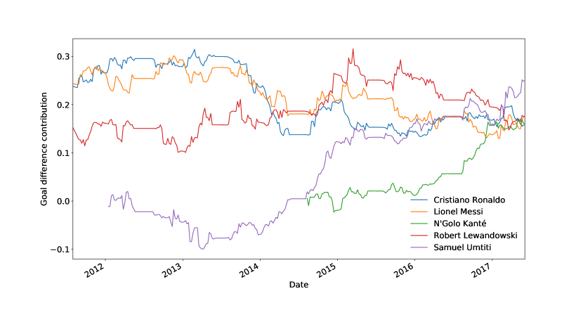
(a) Actual goals plus-minus.

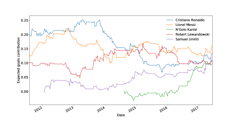
(b) Expected goals plus-minus, xGPM.

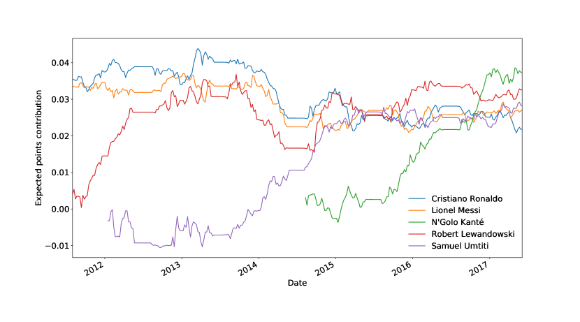
(c) Expected points plus-minus, xPPM.

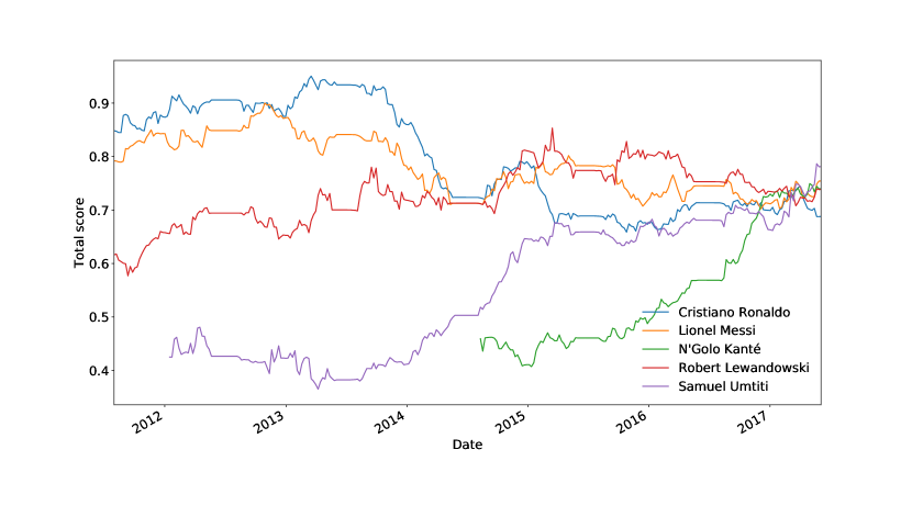
(d) Average of the three plus-minus ratings.

Figure 1: Evolution of the three plus-minus ratings for five example players.

One of the interesting applications of the plus-minus ratings is observing how the performance of selected players has evolved over time. In Figure 1 we plot the relative contributions of Cristiano Ronaldo, Lionel Messi, N’Golo Kanté, Robert Lewandowski and Samuel Umtiti to their respective teams according to each of the three plus-minus ratings: goals PM, xGPM, and xPPM.

We can observe how the three forwards experienced a decline during the 2013/14 season (perhaps they were conserving energy ahead of the 2014 World Cup?), and how the stellar performance of N’Golo Kanté over the last two seasons pushed him to the top of the ratings. In fact, Kanté is top according to both the goals PM and the xPPM, whereas Lionel Messi tops the ratings for xGPM. We also show the mean of the three normalized ratings for illustration and the five players are very similar in value.

5.2.4 Challenging the Ballon D’or Results

The Ballon d’Or is the most prestigious individual distinction in soccer and is awarded to the player deemed to have performed the best over the previous calendar year, based on voting by expert journalists.

Year	Position	Player	Score
2011	1	Andrés Iniesta	0.915
	2	Cristiano Ronaldo	0.914
	3	Pedro	0.906
2012	1	Eden Hazard	0.884
	2	Mirko Vucinic	0.873
	3	Lionel Messi	0.847
2013	1	Gerard Piqué	0.935
	2	Cristiano Ronaldo	0.904
	3	Francesc Fábregas	0.901
2014	1	Manuel Neuer	0.918
	2	Jerome Boateng	0.882
	3	Lionel Messi	0.869
2015	1	David Alaba	0.944
	2	Robert Lewandowski	0.897
	3	Edinson Cavani	0.888
2016	1	N’Golo Kanté	0.915
	2	Claudio Bravo	0.896
	3	Luis Suárez	0.890

Table 5: Top player scores per calendar year

The plus-minus ratings provide us with an alternative way to make a top-player classification for every calendar year. As a proof of concept, we have computed the average of the three variations of the plus-minus rating, each of them previously normalized to the $[0,1]$ range, and filtered out players who didn’t play at least 900 minutes (the equivalent of 10 full games). The results are summarized in Table 5. Despite the fact that the Ballon d’Or award has been dominated by Lionel Messi and Cristiano Ronaldo over the last years our scores suggest that perhaps some other players might have deserved the recognition.

5.2.5 Comparing League Strengths

In this section we examine the results of adjusting for league strength in the PM ratings (Section 4.3). The parameter estimates can be used to compare league strength and this can be used to help clubs understand how players from other leagues might perform in their league. The results are again normalized to the $[0,1]$ range and summarized for each of our PM ratings in Table 6. The final column of the table shows the mean league strength parameter estimate.

	competitionName	PM	xGPM	xPPM	meanPM
1	England Premier League	1.00	0.67	0.97	0.88
2	Germany Bundesliga	0.92	0.32	1.00	0.75
3	Spain La Liga	0.43	1.00	0.49	0.64
4	Italy Serie A	0.61	0.64	0.66	0.64
5	Russia Premier League	0.49	0.52	0.61	0.54
6	Germany Bundesliga II	0.55	0.18	0.86	0.53
7	England Championship	0.63	0.27	0.53	0.48
8	Portugal Liga NOS	0.69	0.00	0.49	0.39
9	France Ligue 1	0.25	0.45	0.18	0.29
10	Turkey Super Lig	0.12	0.10	0.38	0.20
11	Netherlands Eredivisie	0.00	0.32	0.00	0.11

Table 6: League Ranking according to the PM rankings.

The English Premier League dominates the ranking with high scores in goals and points based PM ratings. The second strongest league appears to be the German Bundesliga. The Spanish league scores the highest in terms of expected goals PM but is slightly behind in terms of goals and expected points which may suggest that players trained in this league have a worse conversion ratio (converting opportunities to goals). Surprisingly, the second divisions in Germany and England seem to perform better than the top division in France and Portugal. One possible explanation for this result is that teams get promoted from the second tier divisions in Germany and England and perform better in the top leagues than the players moving from Ligue 1 into these leagues. This may be a result of the players from the second tiers divisions being more familiar with the environment as they have not had to move countries to move leagues. Netherlands seem to be the ‘weakest’ league among the set of leagues we analysed.

6 Conclusions

The paper presents a plus-minus ratings system adapted to soccer. We have proposed two new versions of the plus-minus model designed to react to particular aspects of the game. Our first new plus-minus rating identifies players who change the net expected goals of a team. We have called this the expected goals plus-minus rating, xGPM. The second new plus-minus rating we propose is designed to identify players who change the results of teams by affecting the expected points of a team. We call this rating the expected points plus-minus rating, xPPM.

We have used the new ratings to identify potential alternatives to the Ballon d’Or winner - an award given each year to the best footballer on the planet. We have also used the ratings to examine the evolution of five players’ performances over time. The rise of N’Golo Kante is quite remarkable, and during the 2016-17 season, the models suggest he was the top player in our data (which covers the top leagues in world football). Lastly, we used the model to estimate the relative strengths of the leagues. It appears the English Premier League is slightly stronger than the German Bundesliga, followed by Spain’s La Liga. Somewhat surprisingly, France Ligue 1 is rated as weaker than the second tier divisions in both England and Germany.

Future work may look at using these ratings as part of a forecasting model for match results. Alternatively, to aid those who make decisions regarding team lineups, one could investigate how pairings of players perform together. For example, a coach may be interested in knowing which central defensive pairing is the most effective. For now, we hope that the objectivity of these new ratings and the seemingly ‘expected’ results may mean that plus-minus ratings are used more readily in the soccer industry - both by clubs, fans and the media.

References

- Bates and Maechler, (2017) Bates, D. and Maechler, M. (2017). Matrix: Sparse and Dense Matrix Classes and Methods. R package version 1.2-8.
- Boshnakov et al., (2017) Boshnakov, G., Kharrat, T., and McHale, I. G. (2017). A bivariate Weibull count model for forecasting association football scores. International Journal of Forecasting, 33(2):458–466.
- Brier, (1950) Brier, G. W. (1950). Verification of forecasts expressed in terms of probability. Monthly weather review, 78(1):1–3.
- Brooks et al., (2016) Brooks, J., Kerr, M., and Guttag, J. (2016). Developing a data-driven player ranking in soccer using predictive model weights. In Proceedings of the 22nd ACM SIGKDD International Conference on Knowledge Discovery and Data Mining, pages 49–55. ACM.
- Chen and Guestrin, (2016) Chen, T. and Guestrin, C. (2016). Xgboost: A scalable tree boosting system. CoRR, abs/1603.02754.
- Chollet et al., (2015) Chollet, F. et al. (2015). Keras. https://github.com/fchollet/keras.
- Clarke and Norman, (1995) Clarke, S. R. and Norman, J. M. (1995). Home ground advantage of individual clubs in English soccer. The Statistician, pages 509–521.
- Cox, (1962) Cox, D. R. (1962). Renewal theory, volume 4. Methuen London.
- Dixon and Coles, (1997) Dixon, M. J. and Coles, S. G. (1997). Modelling association football scores and inefficiencies in the football betting market. Journal of the Royal Statistical Society: Series C (Applied Statistics), 46(2):265–280.
- Eggels et al., (2016) Eggels, H., van Elk, R., and Pechenizkiy, M. (2016). Expected goals in soccer: Explaining match results using predictive analytics. In The Machine Learning and Data Mining for Sports Analytics workshop, page 16. Technische Universiteit Eindhoven.
- Fearnhead et al., (2011) Fearnhead, P., Taylor, B. M., et al. (2011). On estimating the ability of NBA players. Journal of quantitative analysis in sports, 7(3):11.
- Friedman et al., (2010) Friedman, J., Hastie, T., and Tibshirani, R. (2010). Regularization paths for generalized linear models via coordinate descent. Journal of Statistical Software, 33(1):1–22.
- Glickman, (2012) Glickman, M. E. (2012). Example of the Glicko-2 system. Boston University.
- Green, (2012) Green, S. (2012). Expected goals in context. optapro-blog.
- Herbrich et al., (2007) Herbrich, R., Minka, T., and Graepel, T. (2007). Trueskill™: A bayesian skill rating system. In Schölkopf, P. B., Platt, J. C., and Hoffman, T., editors, Advances in Neural Information Processing Systems 19, pages 569–576. MIT Press.
- Hunter, (2007) Hunter, J. D. (2007). Matplotlib: A 2d graphics environment. Computing In Science & Engineering, 9(3):90–95.
- Koopman and Lit, (2015) Koopman, S. J. and Lit, R. (2015). A dynamic bivariate Poisson model for analysing and forecasting match results in the English Premier League. Journal of the Royal Statistical Society: Series A (Statistics in Society), 178(1):167–186.
- Liu et al., (2016) Liu, H., Hopkins, W. G., and Gómez, M.-Á. (2016). Modelling relationships between match events and match outcome in elite football. European journal of sport science, 16(5):516–525.
- López Peña and Touchette, (2012) López Peña, J. and Touchette, H. (2012). A network theory analysis of football strategies. In Clanet, C., editor, Sports Physics: Proceedings 2012 Euromech Physics of Sports Conference, pages 517–528. École Polytechnique Paris.
- López Peña and Sánchez Navarro, (2015) López Peña, J. and Sánchez Navarro, R. (2015). Who can replace Xavi? a passing motif analysis of football players. arXiv preprint arXiv:1506.07768.
- Lucey et al., (2014) Lucey, P., Bialkowski, A., Monfort, M., Carr, P., and Matthews, I. (2014). Quality vs quantity: Improved shot prediction in soccer using strategic features from spatiotemporal data. In Proc. 8th Annual MIT Sloan Sports Analytics Conference, pages 1–9.
- Macdonald, (2011) Macdonald, B. (2011). An improved adjusted plus-minus statistic for NHL players. In Proceedings of the MIT Sloan Sports Analytics Conference, URL http://www. sloansportsconference. com.
- (23) Macdonald, B. (2012a). Adjusted Plus-Minus for NHL players using ridge regression with goals, shots, Fenwick, and Corsi. Journal of Quantitative Analysis in Sports, 8(3):1–24.
- (24) Macdonald, B. (2012b). An expected goals model for evaluating NHL teams and players. In Proceedings of the 2012 MIT Sloan Sports Analytics Conference, http://www. sloansportsconference. com.
- Maher, (1982) Maher, M. J. (1982). Modelling association football scores. Statistica Neerlandica, 36(3):109–118.
- McHale and Morton, (2011) McHale, I. and Morton, A. (2011). A Bradley-Terry type model for forecasting tennis match results. International Journal of Forecasting, 27(2):619–630.
- McHale et al., (2012) McHale, I. G., Scarf, P. A., and Folker, D. E. (2012). On the development of a soccer player performance rating system for the English Premier League. Interfaces, 42(4):339–351.
- McHale and Szczepański, (2014) McHale, I. G. and Szczepański, Ł. (2014). A mixed effects model for identifying goal scoring ability of footballers. Journal of the Royal Statistical Society: Series A (Statistics in Society), 177(2):397–417.
- Pedregosa et al., (2011) Pedregosa, F., Varoquaux, G., Gramfort, A., Michel, V., Thirion, B., Grisel, O., Blondel, M., Prettenhofer, P., Weiss, R., Dubourg, V., Vanderplas, J., Passos, A., Cournapeau, D., Brucher, M., Perrot, M., and Duchesnay, E. (2011). Scikit-learn: Machine learning in Python. Journal of Machine Learning Research, 12:2825–2830.
- Pollard, (1986) Pollard, R. (1986). Home advantage in soccer: A retrospective analysis. Journal of Sports Sciences, 4(3):237–248.
- Pollard, (2006) Pollard, R. (2006). Worldwide regional variations in home advantage in association football. Journal of sports sciences, 24(3):231–240.
- Pollard and Pollard, (2005) Pollard, R. and Pollard, G. (2005). Long-term trends in home advantage in professional team sports in north america and england (1876–2003). Journal of Sports Sciences, 23(4):337–350.
- R Core Team, (2016) R Core Team (2016). R: A Language and Environment for Statistical Computing. R Foundation for Statistical Computing, Vienna, Austria.
- Ridder et al., (1994) Ridder, G., Cramer, J. S., and Hopstaken, P. (1994). Down to ten: Estimating the effect of a red card in soccer. Journal of the American Statistical Association, 89(427):1124–1127.
- Rosenbaum, (2004) Rosenbaum, D. T. (2004). Measuring how NBA players help their teams win. 82Games.com (http://www.82games.com/comm30.htm), pages 4–30.
- Sáez Castillo et al., (2013) Sáez Castillo, A., Rodríguez Avi, J., and Pérez Sánchez, J. M. (2013). Expected number of goals depending on intrinsic and extrinsic factors of a football player. an application to professional Spanish football league. European Journal of Sport Science, 13(2):127–138.
- Sill, (2010) Sill, J. (2010). Improved NBA adjusted+/-using regularization and out-of-sample testing. In Proceedings of the 2010 MIT Sloan Sports Analytics Conference.
- Spagnola, (2013) Spagnola, N. (2013). The complete plus-minus: A case study of the Columbus Blue Jackets. Scholar Commons.
- Szczepański and McHale, (2016) Szczepański, Ł. and McHale, I. (2016). Beyond completion rate: evaluating the passing ability of footballers. Journal of the Royal Statistical Society: Series A (Statistics in Society), 179(2):513–533.
- Volf, (2009) Volf, P. (2009). A random point process model for the score in sport matches. IMA Journal of Management Mathematics, 20(2):121–131.
- Winston, (2012) Winston, W. L. (2012). Mathletics: How gamblers, managers, and sports enthusiasts use mathematics in baseball, basketball, and football. Princeton University Press.