The complexity of the Multiple Pattern Matching Problem for random strings

Abstract

We generalise a multiple string pattern matching algorithm, recently proposed by Fredriksson and Grabowski [J. Discr. Alg. 7, 2009], to deal with arbitrary dictionaries on an alphabet of size $s$. If $r_{m}$ is the number of words of length $m$ in the dictionary, and $\phi(r)=\max_{m}\ln(s\,m\,r_{m})/m$, the complexity rate for the string characters to be read by this algorithm is at most $\kappa_{{}_{\textrm{\tiny UB}}}\,\phi(r)$ for some constant $\kappa_{{}_{\textrm{\tiny UB}}}$.
 On the other side, we generalise the classical lower bound of Yao [SIAM J. Comput. 8, 1979], for the problem with a single pattern, to deal with arbitrary dictionaries, and determine it to be at least $\kappa_{{}_{\textrm{\tiny LB}}}\,\phi(r)$. This proves the optimality of the algorithm, improving and correcting previous claims.

1 The problem

1.1 Definition of the problem

Let $\Sigma$ be an alphabet of $s$ symbols, $\xi=(\xi_{1},\ldots,\xi_{n})\in\Sigma^{n}$ a word of $n$ characters (the input text string), $D=\{w_{1},\ldots,w_{k}\}$, $w_{i}\in\Sigma^{*}$ a collection of words (the dictionary). We say that $w$ occurs in $\xi$ at position $j$ if $w\equiv\xi_{j}\xi_{j+1}\cdots\xi_{j+|w|-1}$. Let $r_{m}(D)$ be the number of words of length $m$ in $D$. We call ${\bm{r}}(D)=\{r_{m}(D)\}_{m\geq 1}$ the content of $D$, a notion of crucial importance in this paper.

The multiple string pattern matching problem (MPMP), for the datum $(D,\xi)$, is the problem of identifying all the occurrences of the words in $D$ inside the text $\xi$ (cf. Figure 1).

A version of the problem can be defined in the case of infinite dictionaries ($k=\infty$), where, as we may assume that all the words of the dictionary are distinct, we can suppose that $r_{m}\leq s^{m}$. The analysis of the present paper treats in an unified way the case of finite and infinite dictionaries.

The first seminal works have concerned single-word dictionaries. Results included the determination of the average complexity of the problem, the design of efficient algorithms (notably Knuth-Morris-Pratt and Boyer-Moore), and have led to the far-reaching definition of Aho-Corasick automata [3, 4, 5, 6].

$\xi$	501011 1000100 1500100 2010101 2510101 3001000 3511100 4010110 45
$D$	110010101100100001001010110101010001110010110	output
0010	..*---....*---.*--*---................*---...	$3,11,16,19,39$
01010	...*----...........*----..*-*----............	$4,20,27,29$
1011001	......*------................................	7

Figure 1: Typical output of a multiple string pattern matching problem. In this case $s=2$ and ${\bm{r}}(D)=(0,0,0,1,1,0,1,0,\ldots)$.

The computational complexity of the problem, for a given dictionary $D$, in worst case among texts $\xi$ of length $n$, is a problem solved by Rivest long ago [7], with a deceivingly simple answer (within our complexity paradigm, based on text accesses, see below): for each word, there exist texts that need to be read entirely.

On the other side, the average-case analysis, over texts $\xi$ sampled uniformly in $\Sigma^{n}$ (in the limit of large $n$) is an interesting problem, and its determination for any given dictionary $D$ is the ideal goal of this paper.

Unfortunately, the exact determination of the complexity for an arbitrary dictionary seems a formidable task, and we have to revert to a more concrete challenge. More precisely, our goal is as follows.

• Analogously to what is done in Knuth, Morris and Pratt [5] and in Yao [6], we do not analyse the time complexity, but rather the complexity in terms of character accesses to original text.

• The asymptotic complexity is $\Theta(n)$, in other words there exists some constant $\Phi(D)$ such that the quantity of interest is $\Phi(D)\,n+o(n)$. Again, analogously to previous literature, instead of determining the quantity $\Phi(D)$ exactly, we determine the functional dependence of $\Phi$ from $D$, up to a finite multiplicative constant, and thus produce upper and lower bounds whose ratio is uniformly bounded.

We now describe in more detail the subtleties of the forementioned complexity paradigm.

Let $m_{\rm min}$ be the length of the shortest pattern in $D$. In particular, the number of character accesses is at most $n$, the case in which the whole text is read, and is $n-\mathcal{O}(1)$ in worst case. It is also at least $n/m_{\rm min}+\mathcal{O}(1)$, because one needs to read at least one character out of $m_{\rm min}$ consecutive ones. Another trivial consequence is that we can restrict to the case $m_{\rm min}\geq 2$, as, if we have even a single word in $D$ of length 1, we know in advance that the whole text needs to be read.

The average number of characters to be read for texts of length $n$ is a super-additive sequence (because solving an instance $\xi$ of size $n_{1}+n_{2}$ is harder than solving the two instances, of sizes $n_{1}$ and $n_{2}$, associated to the appropriate prefix and suffix of $\xi$). As a consequence of Fekete’s Subadditive Lemma, the limit fraction of required character comparisons exists and is equal to the lim-sup of the same quantity. The Fekete’s Lemma in itself leaves open the possibility that the limit is infinite, however from the forementioned trivial upper bound we can conclude that this limit is a finite constant associated to the dictionary.

We introduce the quantity $\Phi(D)$, by defining this fraction to be $\Phi(D)/\ln s$, and we have thus determined that

$$\frac{\ln s}{m_{\rm min}(D)}\leq\Phi(D)\leq\ln s\,.$$

The presence of the logarithmic prefactor is a useful convention, associated to the fact that reading $N$ characters in a $s$-symbol alphabet gives a $N\log_{2}(s)$ amount of Shannon information entropy (we further use natural basis for logarithms, in order to simplify the calculations). An advantage of the rescaled quantity is the fact that it has a form of stability under reduction of the text into $q$-grams (i.e., a text of length $qn$ on an alphabet $\Sigma$ of $s$ symbols has the same Shannon entropy, $(nq)\log_{2}(s)=n\log_{2}(s^{q})$, of the text of length $n$ consituted of symbols in $\Sigma^{q}$). Our ideal task would be the determination of $\Phi(D)$.

Yao [6] determines in particular that, if $D$ consists of a single word of length $m$, when $1\ll m\ll n$, the complexity above is given by a certain expression in $m$ and $s$, up to a finite multiplicative constant, for almost all patterns, i.e. for almost all of the $s^{m}$ possible words of the given length. Patterns with a different complexity, in fact, always have a smaller complexity, i.e. it is not excluded that there are a few atypically-simpler words, while it is established that there are no (significantly) atypically-harder ones. In analogy to this result, it is natural to imagine that, as we will see in the following, almost all dictionaries with the same content ${\bm{r}}$ have the same complexity up to finite multiplicative factors, and the few remaining ones have a smaller complexity. For this reason we find interesting to define

$$\Phi_{\rm min}({\bm{r}}) :=\min_{D}\Phi(D)\,;$$ (1)

$$\Phi_{\rm aver}({\bm{r}}) :=\mathbb{E}_{D}\big{(}\Phi(D)\big{)}\,;$$ (2)

$$\Phi_{\rm max}({\bm{r}}) :=\max_{D}\Phi(D)\,;$$ (3)

where min, max and average are taken over $D$ such that ${\bm{r}}(D)={\bm{r}}$, and one of our aims is to prove that $\Phi_{\rm aver}({\bm{r}})$ and $\Phi_{\rm max}({\bm{r}})$ functions have the same behaviour up to a multiplicative constant (while this is not the case for $\Phi_{\rm min}({\bm{r}})$).

Also the exact determination of $\Phi_{\rm aver}({\bm{r}})$ and $\Phi_{\rm max}({\bm{r}})$ is an overwhelming task. We will content ourself of a determination of these functions up to a multiplicative constant, i.e. the identification of a function $\phi({\bm{r}})$, and a constant $\kappa$, such that

$$\frac{\phi({\bm{r}})}{\kappa}\leq\Phi_{\rm aver}({\bm{r}})\leq\Phi_{\rm max}({\bm{r}})\leq\kappa\,\phi({\bm{r}})\,.$$ (4)

Yet again, this is not dissimilar to what is done in the seminal Yao paper.

Note that the average in $\Phi_{\rm aver}({\bm{r}})$ allows for the repetition of the same word in the dictionary, and for the presence of pairs of words in the dictionary which are one factor of the other. These problems are thus trivially reduced to problems on a smaller dictionary. If we call $\Phi^{\prime}_{\rm aver}({\bm{r}})$ the average performed while excluding these degenerate cases, from the monotonicity of the complexity as a function of $D$ (w.r.t. inclusion) we get that $\Phi_{\rm aver}({\bm{r}})\leq\Phi^{\prime}_{\rm aver}({\bm{r}})\leq\Phi_{\rm max}({\bm{r}})$, so that our theorem, as a corollary, establishes the behaviour of the more interesting quantity $\Phi^{\prime}_{\rm aver}({\bm{r}})$. Observe that it is legitimate to do this even while still keeping the bound $r_{m}\leq s^{m}$, which occurs only in problems without repetitions, because we are comparing the two types of averages while the content ${\bm{r}}$ is kept fixed.

We shall comment on the fact that finding the complexity up to a multiplicative constant is not an easy task a priori. Suppose that we have a concrete working strategy to determine an upper bound for a given vector ${\bm{r}}$, and a second strategy to determine a lower bound for given ${\bm{r}}$. Then one may naïvely think that $\kappa$ is related to the maximum, over all ${\bm{r}}$, of the associated ratio. This idea is wrong, because the space of possible ${\bm{r}}$ is not a compact, and the ‘maximum’ of this ratio is in fact a ‘supremum’, which may well be infinity. So, any valid lower and upper bounds provide an estimate of the complexity for a given content ${\bm{r}}$ up to a constant, but we need “good” bound strategies in order to capture the full functional dependence of the complexity from the content parameters ${\bm{r}}=\{r_{m}\}$.

1.2 The result and its implications

Let

$$\phi({\bm{r}}):=\max_{m}\frac{1}{m}\ln(s\,m\,r_{m})\,.$$ (5)

Note that, even in the case of infinite dictionaries $D$, with all words of length at least $m_{\rm min}$, $\phi({\bm{r}}(D))$ must evaluate to a finite value, as it is bounded by $\ln s+\frac{1}{m_{\rm min}}\ln(s\,m_{\rm min})$ (because $r_{m}\leq s^{m}$).

Our aim is to prove the following theorem, valid in the interesting regime $s\geq 2$ and $m_{\rm min}\geq 2$.

Theorem 1

Let $\kappa_{s}=5\frac{\sqrt{s}}{\ln s}$. For all contents ${\bm{r}}$, the complexity of the MPMP on an alphabet of size $s$ satisfies the bounds

$$\frac{1}{\kappa_{s}}\left(\phi({\bm{r}})+\frac{1}{2s\,m_{\rm min}}\right)\leq\Phi_{\rm aver}({\bm{r}})\leq\Phi_{\rm max}({\bm{r}})\leq 2\left(\phi({\bm{r}})+\frac{1}{2s\,m_{\rm min}}\right)\,.$$ (6)

As a corollary, by using

$$0\leq\frac{1}{m_{\rm min}}\leq\frac{1}{\ln 4}\frac{\ln(s\,m_{\rm min}r_{m_{\rm min}})}{m_{\rm min}}\leq\frac{1}{\ln 4}\phi({\bm{r}})\,,$$ (7)

from (6) we can deduce bounds in a weaker but functionally simpler form

$$\frac{1}{\kappa_{s}}\phi({\bm{r}})\leq\Phi_{\rm aver}({\bm{r}})\leq\Phi_{\rm max}({\bm{r}})\leq\bigg{(}2+\frac{1}{\ln 4}\bigg{)}\phi({\bm{r}})\,,$$

i.e. the whole fuctional dependence from the dictionary is captured by the function $\phi$, up to a multiplicative factor depending only on $s$, and bounded by $\sim 13.6\frac{\sqrt{s}}{\ln s}$.

The reader may be wondering why the function $\phi({\bm{r}})$ is the ‘good one’ to capture the behaviour of the complexity. We cannot give a full intuition of this feature without entering in the details of the calculations. Nonetheless, we can remark that $\phi({\bm{r}})$ is defined as a maximum over $m$, of a function of $m$ and $r_{m}$ alone. As a result, from the statement of the theorem we deduce the following striking property. Let $D$ be a dictionary for the generic MPMP, with content ${\bm{r}}=\{r_{m}\}_{m\geq 2}$. Let $m^{*}$ be any argmax of the function entering the definition of $\phi$, for such a ${\bm{r}}$, and let $D^{\prime}$ be the dictionary corresponding to the restriction of $D$ only to the words with length $m^{*}$, plus a single word of length $m_{\rm min}$ (if $m_{\rm min}\neq m^{*}$). As the functions $\phi({\bm{r}}(\cdot))$ and $1/m_{\rm min}$ evaluate to the same values for $D$ and $D^{\prime}$, we have thus determined that $\Phi(D)/\Phi(D^{\prime})\leq\kappa^{2}$, i.e. the pruned dictionary has a complexity not sensibly smaller than the original one, despite the fact that the space of possible $D$’s is not compact, and, even worse, $D$ may consist of an infinite dictionary.

This may sound surprising, as one could have expected that, when $m^{*}$ is large, the function $\frac{1}{m}\ln(s\,m\,r_{m})$ may well be almost flat in an interval whose width scales with $m^{*}$ (e.g., between $\frac{1}{2}m^{*}$ and $2m^{*}$), and, as a result, $D$ has many more words than $D^{\prime}$. One may have expected that the worst-case ratio $\Phi(D)/\Phi(D^{\prime})$ showed a non-trivial functional dependence from $m^{*}$ under such circumstances, e.g. a factor related to the width of such window, but this is not the case, although, yet again, we cannot explain why without entering the detailed analysis of the proof.

Let us make one last comment on the structure of the theorem. Our goal is the determination of the functional dependence of $\Phi(D)$ up to a finite multiplicative constant. From the forementioned trivial bounds $\frac{1}{m_{\rm min}}\ln(s)\leq\Phi(D)\leq\ln(s)$, we see that this goal only makes sense when the ratio between the two trivial bounds is large, and there is no point in analysing dictionaries in which $m_{\rm min}$ is smaller than this constant.

As a further corollary, there is no point in considering dictionaries which do not have complexity $o(1)$ w.r.t. some size parameter. It is not hard to see that such dictionaries exist, even with simple arguments unrelated to our analysis.

The fact that ‘interesting’ dictionaries have all words ‘sufficiently long’ leads to a leitmotif of our analysis (which also appears transversally in most of the mentioned literature). In the construction of the bounds we are led to analyse complicated functions $f(m)$, e.g. the solution of a transcendental equation. In order to work out our results, we will just need that we can estimate upper and/or lower bounds to this function, which are ‘effective’ in a regime of $m$ large, even if they are quite poor for $m$ too small. As we will see, most functions $f(m)$ occurring in this problem will allow for a perturbative expansion in powers of $(\ln m)/m$.

1.3 Previous results

Single-word dictionaries. The statement of Theorem 1 restricted to single-word dictionaries is related to the result of the seminal paper of Yao [6]. In this case, in $\phi$ there is no need to take a $\max$, and $r_{m^{\prime}}=1$ for $m=m^{\prime}$ and $0$ otherwise. While our theorem gives that, for such a ${\bm{r}}$, in worst case among words of length $m$,

$$\frac{1}{\kappa_{s}}\left(\frac{\ln(s\,m)+\frac{1}{s}}{m}\right)\leq\Phi({\bm{r}})\leq 2\left(\frac{\ln(s\,m)+\frac{1}{s}}{m}\right)\,,$$

Yao determines that for almost all words of length $m$, and treating $s$ as a constant, the complexity is $\Theta(\frac{\ln(m)}{m})$. In order to establish this result, Yao introduces a notion of certificate. The set $C\subseteq\{1,\ldots,n\}$ is a certificate for the pair $(D,\xi)$ if the knowledge of $\{\xi_{j}\}_{j\in C}$ completely determines the output of the problem (in fact, Yao defines certificates only for single-word dictionaries, but the generalised notion is evinced in a natural way). Call $\mathcal{C}(D,\xi)$ the set of certificates, and define

$$\Phi_{\rm cert}(D,\xi):=\frac{\ln s}{n}\min_{C\in\mathcal{C}(D,\xi)}|C|\,,$$ (8)

together with the average quantities

$$\Phi_{\rm cert}(D):=\mathbb{E}_{\xi}\big{(}\Phi_{\rm cert}(D,\xi)\big{)}\,;$$ (9)

and

$$\Phi_{\rm cert}({\bm{r}}):=\mathbb{E}_{D\,:{\bm{r}}(D)={\bm{r}}}\big{(}\Phi_{\rm cert}(D)\big{)}\,.$$ (10)

This is another natural notion of complexity for MPMP, that we shall call the certificate complexity of the instance. It is the smallest possible complexity of the given instance, or, in other words, it is the smallest complexity among all possible runs of the probabilistic algorithm, that reads the characters of the text one by one in a random order, up to when a certificate is reached.

This notion is a lower bound to the ‘true’ complexity of the instance, just because any algorithm (and any run of a non-deterministic algorithm) may halt only when a certificate is reached. Intuitively, reaching the value $\Phi_{\rm cert}(D,\xi)$ supposes not only (or better, not necessarily) the optimality of the algorithm, but also an infinite amount of ‘luck’ in the choice of the characters to read, given the hidden text $\xi$, from which the inequality would follow.

Thus the analysis of $\Phi_{\rm cert}$ provides a natural proof strategy for what concerns the estimate of a lower bound, that Yao succeeds in pursuing for the single-word case, and that, in this paper, we adapt to the case of general dictionaries.

As a side remark, it is natural to conjecture, although we suppose hard to prove in full generality, that $\Phi_{\rm cert}(D)<\Phi(D)$, i.e. that the necessity of ‘infinite luck’ is intrinsic to the definition and cannot be compensated by the optimisation of the algorithm. This can be established rigorously, for example, for $\Sigma=\{{\tt a},{\tt b}\}$ and dictionary $D=\{{\tt ab}\}$, for which one can determine that the Boyer–Moore algorithm is optimal, and has information complexity $\Phi=5/6$, while the certificate complexity is $\Phi_{\rm cert}=13/16$, which is smaller by a tiny amount, roughly $2\%$ (we do not illustrate this interesting fact here, as it would be a détour w.r.t. our main aim). The gap between the two complexities is expected to become increasingly smaller as the dictionary gets larger, this making the forementioned conjecture more challenging.

Uniform dictionaries. Let us say that a dictionary $D$ is uniform if all the words have the same length. Fredriksson and Grabowski [8] describe a MPMP algorithm (in the following, the FG algorithm) adapted to deal with uniform dictionaries, and analyse the resulting upper bound. This algorithm is possibly never optimal (and known to be non-optimal on certain simple dictionaries), but the loss is by a relatively small factor, and, in many applications, is compensated by a great simplicity both in programming and in the statistical analysis. Based on previous results of Fredriksson and Navarro [9], that purportedly estimated lower bounds for uniform dictionaries, the authors claimed their algorithm to be optimal up to multiplicative factor, in its domain of contents ${\bm{r}}$, and provided a complexity compatible with the corresponding specialisation of our theorem above. However, the results of [9] are invalidated by a major flaw (and thus the optimality result in [8] remained unproven before the present paper). For this reason, our lower-bound estimate, for dictionaries of arbitrary content, is completely different from the one in [9], while it is in fact mostly an adaptation of the original strategy of Yao [6] for single-word dictionaries.

This lower bound is presented in Section 4, while the adaptation of the FG algorithm, and the resulting upper bound, are outlined in Sections 2 and 3, respectively.

2 The Fredriksson–Grabowski algorithm

As we mentioned, ideally we want an algorithm with a degree of flexibility, such that, in the interesting cases $m_{\rm min}\gg 1$, a fraction $\ll 1$ of the text is accessed, i.e. some ‘big jumps’ are performed. The idea of Fredriksson and Grabowski [8] is to encode this flexibility in a single parameter $q$ associated to a dilution rate of the words in the dictionary.

For a fixed integer $q$, a text $\xi$ and a dictionary $D=\{w_{j}\}_{1\leq j\leq k}$, define the diluted text $\xi^{(q)}=(\xi_{q},\xi_{2q},\xi_{3q},\ldots)$ and the diluted dictionary $D^{(q)}=\{w_{j,p}\}_{1\leq j\leq k,\;0\leq p<q}$. For a word $w_{j}$ of length $m$, call $w_{j}^{1}$, …, $w_{j}^{m}$ its $m$ characters. If $|w_{j}|=m_{j}$, $w_{j,p}$ is defined as

$$w_{j,p}=w_{j}^{m_{j}-p-hq}\cdots w_{j}^{m_{j}-p-q}w_{j}^{m_{j}-p}\qquad h=\lfloor(m_{j}-p-1)/q\rfloor\,.$$

For example, if $w_{1}=\textrm{\tt thepattern}$ and $q=3$, the three words $w_{1,0}$, $w_{1,1}$ and $w_{1,2}$ are obtained by the sieve construction

t h e p a t t e r n
t . . p . . t . . n	tptn
. . e . . t . . r .	etr
. h . . a . . e . .	hae

Call $[m/q]_{p}:=\lfloor\frac{m-p-1}{q}\rfloor+1$. Then $|w_{j,p}|=[|w_{j}|/q]_{p}$.

Let us denote by $\mathrm{FG}(q)$ the algorithm of parameter $q$, and by $\Phi_{\mathrm{FG}(q)}(D)$ the upper bound to $\Phi(D)$ obtained by analysing this algorithm. The FG algorithm of parameter $q$, in its simplest version, consists in reading the characters of $\xi^{(q)}$ in sequence, and searching for words in the dictionary $D^{(q)}$. Once an occurrence has been found, it reads the missing $m\frac{q-1}{q}+\mathcal{O}(1)$ characters in order to verify if the original word was present. This idea can be improved at various extents. For example, once we have agreed to solve the MPMP $(D^{(q)},\xi^{(q)})$, nothing prevents from using a ‘good’ algorithm for this, and possibly, just recursively the FG algorithm, instead of switching to the naïve read-all algorithm. Furthermore, instead of just filling the whole gap, we can just proceed to read the characters of the gap one by one, and stop the procedure if a contradiction with the candidate word is found (for future reference, let us call this sharp gap filling). However it turns out that, at the aim of determining $\Phi(D)$ up to multiplicative constants, these improvements are not crucial. See Figure 2 for an example.

Figure 2: A typical realisation of the Fredriksson–Grabowski algorithm. Dotted entries will not be read. In its basic implementation, analysed here, it is the a at the far right that excludes the decimated pattern etr. A more efficient variant, but more complicated to analyse, would find that the pattern etr is excluded by the $\xi_{i}$’s already read at the previous step.

In the (non-improved) $\mathrm{FG}(q)$ algorithm, we read at least a fraction $1/q$ of the text, and, as it will turn out, for the optimal value of $q$ the total fraction is slightly above $1/q$. If a dictionary $D$ has its shortest word of length $m_{\rm min}$, the complexity of any algorithm is at least $1/m_{\rm min}$, so, under the ansatz above, there is no point in searching among values $q>m_{\rm min}$, and in particular there are no empty words in $D^{(q)}$.

The exact value of $\Phi_{\mathrm{FG}(q)}(D)$ is hardly expressed by a closed formula, because we may be forced to fill the same gap by more than one occurrence of diluted words. These characters shall count only once in the complexity, but the interplay of different words in the dictionaries is complicated to analyse. So, we will content ourselves with the upper bound to this complexity obtained from the union bound (Boole’s inequality) on these occurrences:

Proposition 2

$$\Phi_{\mathrm{FG}(q)}(D)\leq\frac{\ln s}{q}\bigg{(}1+\sum_{m}r_{m}\sum_{p=0}^{q-1}s^{-[m/q]_{p}}(m-[m/q]_{p})\bigg{)}\,.$$ (11)

Proof. The formula above is deduced from an easy reflection on the mechanisms of the algorithm. We read one in $q$ characters, to solve the diluted problem with the trivial read-all algorithm (from which the $1/q$ factor). Then, at each position of the diluted string, if we find a candidate subpattern $w_{j,p}$, we read the missing $|w_{j}|-|w_{j,p}|$ characters (from which the $(m-[m/q]_{p})$ factor). This gives an overcounting (by union bound) when we find more than one subpattern at the same position, or at a short distance along the diluted text, but it makes the probabilities of finding subpatterns independent, and thus just given by the obvious factor $s^{-|w_{j,p}|}$, this being an important simplification to the formula, relevant in the following calculations.

Note how, just by the use of the read-all algorithm on the diluted subproblem, and the union bound on the occurrences in this subproblem, we have determined an upper bound on $\Phi_{\mathrm{FG}(q)}(D)$ that depends on $D$ only through its content ${\bm{r}}(D)$. This upper bound on the complexities of all variants of the FG algorithm discussed above is in fact the exact complexity of the most naïve version of the algorithm, the one in which, if more than one word of $D^{(q)}$ is found at a given diluted position, the missing characters are accessed multiple times, and these multiple accesses are counted with their multiplicities.

If we perform the ‘sharp gap filling’ enhancement discussed above, i.e. we stop to read characters in the verification of a given candidate sub-pattern whenever we obtain a contradiction, we can replace the factor $m^{\prime}:=m-[m/q]_{p}$ in (11), i.e. the maximal number of read characters for the diluted pattern, by the expectation of read characters, which is

$${\textstyle\frac{s-1}{s}}\left(1+{\textstyle\frac{2}{s}}+{\textstyle\frac{3}{s^{2}}}+\cdots+{\textstyle\frac{m^{\prime}-1}{s^{m^{\prime}-2}}}\right)+{\textstyle\frac{m^{\prime}}{s^{m^{\prime}-1}}}={\textstyle\frac{s}{s-1}}(1-s^{-m^{\prime}})$$ (12)

getting the improved expression

Proposition 3

$$\Phi_{\mathrm{FG}(q)}(D)\leq\frac{\ln s}{q}\bigg{(}1+\frac{s}{s-1}\sum_{m}r_{m}\sum_{p=0}^{q-1}\big{(}s^{-[m/q]_{p}}-s^{-m}\big{)}\bigg{)}\,.$$ (13)

3 The upper bound

We shall now analyse the expression on the RHS of the inequality (11) – or better, the inequality (13) improved by the sharp gap filling – in order to produce a more compact expression for an upper bound to the complexity, and, in agreement with Theorem 1, prove the following

Proposition 4

With $\phi({\bm{r}})$ as in equation (5), we have

$$\Phi_{\rm max}({\bm{r}})\leq 2\phi({\bm{r}})+\frac{1}{s\,m_{\rm min}}\,.$$ (14)

As we have $\Phi(D)\leq\Phi_{\mathrm{FG}(q)}(D)$ for any value of $q$, we have in particular $\Phi(D)\leq\Phi_{\mathrm{FG}(q({\bm{r}}(D)))}(D)$ for any integer-valued function $q({\bm{r}})$, the best choice being the value of $q$ minimising the expression on the RHS of (13), for the given ${\bm{r}}$. We shall provide a function $q({\bm{r}})$ which, although not being exactly the minimum, is sufficiently close to this value that our upper and lower bounds, as functions of ${\bm{r}}$, match up to a finite multiplicative constant. However, this condition can only be verified a posteriori, once that a lower bound, of functional form analogous to the RHS of (14), is established, so in this section we shall content ourselves with the analysis of the resulting expression, leaving our choice of $q({\bm{r}})$ as an ansatz.

Proof of Proposition 4. Let us start from the improved expression (13). Let us drop the summands $-s^{-m}$, and get the slightly larger bound

$$\Phi_{\mathrm{FG}(q)}(D)\leq\frac{\ln s}{q}+\frac{s\ln s}{s-1}\sum_{m}r_{m}\frac{1}{q}\sum_{p=0}^{q-1}s^{-[m/q]_{p}}\,.$$ (15)

Let us concentrate on the inner-most expression

$$f(s;m,q):=\frac{1}{q}\sum_{p=0}^{q-1}s^{-[m/q]_{p}}\,.$$ (16)

Writing $m=aq+b$ with $0\leq b<q$, this just reads

$$f(s;aq+b,q):=s^{-a}\frac{bs^{-1}+q-b}{q}\,.$$ (17)

This function can be analytically extended, in terms of

$$g(s,x):=s^{x}\big{(}xs^{-1}+1-x\big{)}$$ (18)

because

$$f(s;m,q)=s^{-\frac{m}{q}}g(s,b/q)\,.$$ (19)

For $s>0$, the function $g(s,x)$ is concave on $[0,1]$, its only maximum is at $x^{*}(s)=1+\frac{1}{s-1}-\frac{1}{\ln s}$, where one has $g^{*}(s)=g(s,x^{*}(s))=\frac{s-1}{\ln s}\exp\big{(}\frac{\ln s}{s-1}-1\big{)}$. In particular, for $s\geq 2$ we have $g^{*}(s)\leq\frac{2}{e}\frac{s-1}{\ln s}$. Substituting into (15) gives

$$\Phi_{\mathrm{FG}(q)}(D)\leq\frac{\ln s}{q}+\frac{2s}{e}\sum_{m}r_{m}s^{-\frac{m}{q}}\,.$$ (20)

The change of variables $\rho=\frac{\ln s}{q}$ gives

$$\begin{split}&\Phi_{\mathrm{FG}(q)}(D)\leq\rho+\frac{2s}{e}\sum_{m}r_{m}e^{-m\rho}=\rho+\frac{2}{es}\sum_{m\geq m_{\rm min}}\frac{e^{-m\big{(}\rho-\frac{\ln(s^{2}m^{2}r_{m})}{m}\big{)}}}{m^{2}}\,.\end{split}$$ (21)

Now choose the candidate value $\rho=2\phi({\bm{r}})$, that is, $q({\bm{r}})=\ln s/(2\phi({\bm{r}}))$, with $\phi({\bm{r}})$ as in equation (5). We have $\rho\geq\frac{2\ln(smr_{m})}{m}\geq\frac{\ln(s^{2}m^{2}r_{m})}{m}$ for all $m$, so that

$$\begin{split}&\sum_{m\geq m_{\rm min}}\frac{e^{-m\big{(}\rho-\frac{\ln(s^{2}m^{2}r_{m})}{m}\big{)}}}{m^{2}}\leq\sum_{m\geq m_{\rm min}}\frac{1}{m^{2}}\leq\frac{\pi^{2}-6}{3}\frac{1}{m_{\rm min}}\,,\end{split}$$

(where we used the result of Appendix A). As $\frac{2}{e}\frac{\pi^{2}-6}{3}<1$, we can write

$$\Phi_{\mathrm{FG}(\ln s/(2\phi({\bm{r}})))}({\bm{r}})\leq 2\phi({\bm{r}})+\frac{1}{s\,m_{\rm min}}\,.$$ (22)

This allows us to conclude. $\square$

4 The lower bound

In this section we establish a lower bound on the complexity, averaged over all dictionaries of content ${\bm{r}}$, of the form

Proposition 5

For $s\geq 2$, define $\kappa_{s}=5\frac{\sqrt{s}}{\ln s}$. In the MPMP on an alphabet of size $s$,

$$\Phi_{\rm aver}({\bm{r}})\geq\Phi_{\rm cert}({\bm{r}})\geq\frac{1}{\kappa_{s}}\left(\phi({\bm{r}})+\frac{1}{2s\,m_{\rm min}}\right)\,.$$ (23)

4.1 Reduction to a finite text

In evaluating a lower bound on the information complexity of MPMP, it is legitimate to replace the exact expression by simpler quantities which bound it from below. The goal is to reach a concretely evaluable expression, without losing the leading functional dependence from $D$ (up to multiplicative constants), or, better, the dependence from ${\bm{r}}(D)$.

The output of a MPMP is a list of pairs $S(D,\xi)=\{(\ell,h)\}$, with $1\leq h\leq k$ and $1\leq\ell\leq n-|w_{h}|+1$, such that $w_{h}$ occurs at position $\ell$ in the text. Call $X_{0}=\{(\ell,h)\,|\,1\leq h\leq k\,;\,1\leq\ell\leq n-|w_{h}|+1\}$ the list of possible pairs described above. If we specify in advance a subset $X\subseteq X_{0}$, and decide that we aim at finding all the occurrences within this subset, we have a reduced problem with complexity, say, $\Phi(D|X)$ (while the complexity of the original problem is $\Phi(D)\equiv\Phi(D|X_{0})$). The problem associated to the subset $X$ is evidently simpler than the original one, at least within our notion of complexity (in terms of text characters to be read): a solution $S(D,\xi)$ of the full problem provides a solution of the reduced one, just by taking the intersection $S(D,\xi)\cap X$, and this process does not involve further accesses to the text, thus we have $\Phi(D|X)\leq\Phi(D)$ for all $X\subseteq X_{0}$. A similar argument applies to the certificate complexity. Thus, this observation provides a useful strategy for producing lower bounds for both versions of the complexity.

As it was the case for the upper bound and the parameter $\rho$, we need a free real parameter in order to capture the functional dependence from $D$. In analogy to Yao procedure, a good choice is an integer $L$, which determines a set $X=X(L)$ as follows:

$$X(L)=\left\{(\ell,h)\,\bigg{|}\,\left\lfloor\frac{\ell+1}{L}\right\rfloor=\left\lfloor\frac{\ell+|w_{h}|}{L}\right\rfloor\right\}\,.$$ (24)

In simple words, the text, originally of length $n$, is divided into blocks of size $L$ (with the possible exception of one last block of size $<L$), and we search for occurrences contained within one block. As a result of this bound, we have factorised the problem on the blocks, and the calculation of (the bound on) the complexity rate, i.e. the limit of $1/n$ times the complexity, for $n\to\infty$, is given by $1/L$ times the whole average complexity of single blocks, again both for ordinary and certificate complexities.

$$\Phi(D) \geq\mathbb{E}_{\xi\in\Sigma^{L}}\Phi(D,\xi)\,; \Phi_{\rm cert}(D) \geq\mathbb{E}_{\xi\in\Sigma^{L}}\Phi_{\rm cert}(D,\xi)\,; \forall\ L\,.$$ (25)

This solves the issue of performing the limit $n\to\infty$, and reduces to a problem which, for a fixed dictionary, is of finite size, namely $L$ (although, in fact, the optimal value of $L$ as a function of $D$ is unbounded). From this moment on, we can thus concentrate on a single block.

It is rather clear that we need $L$ to be not below the scale $m^{*}(D)$ of the most relevant word-length for the given dictionary, otherwise we would just miss the totality of the occurrences which give the leading term of the complexity. Surprisingly, it will turn out that the optimal value of $L$ is barely above $m^{*}$.

4.2 The lattice of possible algorithms

Under our complexity paradigm, and for a fixed text $\xi$ of length $L$, we can visualise any algorithm as a recipe for performing a directed walk on the lattice of subsets $I$ of $\{1,\ldots,L\}$.

Any algorithm starts at the bottom of the lattice, i.e. the node associated to the empty subset. The algorithm evaluates a function of $D$, in order to choose a position $1\leq i_{1}\leq L$ to access. Then, it reads $\xi_{i_{1}}$, thus ‘moving’ to the set $\{i_{1}\}$, and it evaluates a function of $D$ and $\xi_{i_{1}}$, in order to choose a position $i_{2}\neq i_{1}$. Then, it reads $\xi_{i_{2}}$, thus moving to $\{i_{1},i_{2}\}$, and chooses a position $i_{3}\neq i_{1},i_{2}$ through a function of $D$ and $\{\xi_{i_{1}},\xi_{i_{2}}\}$, and so on, until a certificate is reached (see Figure 3). We say that the algorithm, at a certain moment of its execution, is at the node $I=\{i_{1},\ldots,i_{t}\}$ of the lattice, if, so far, it has accessed the text characters at positions $\{i_{1},\ldots,i_{t}\}$ (in any of the possible orders). The nodes are associated to unordered sets of positions, instead that of ordered lists, because there is no reason why the function of $D$ and $\{\xi_{i_{1}},\ldots,\xi_{i_{t}}\}$ shall depend on the order in which the positions $\{i_{1},\ldots,i_{t}\}$ have been accessed: any such dependence would only make the algorithm less performing.

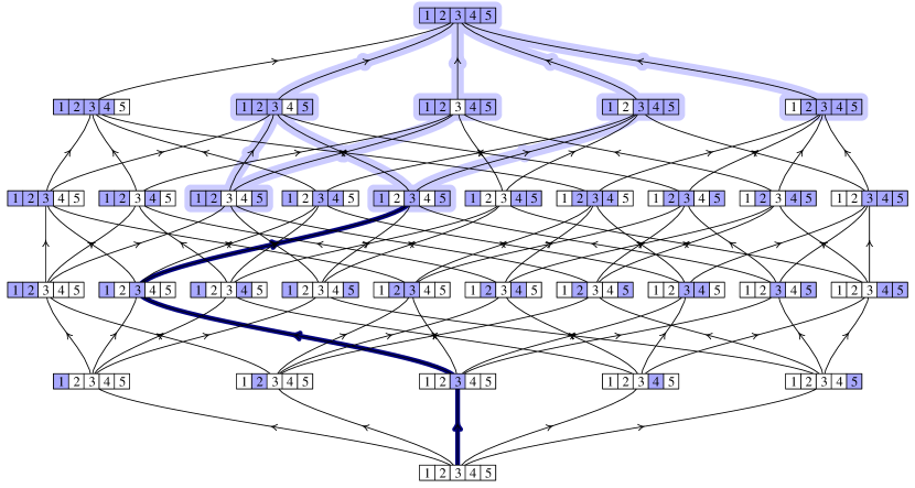
Figure 3: The lattice of subsets of $\{1,\ldots,5\}$. The shadowing denotes an example of up-set, corresponding, for a certain pair $(D,\xi)$, to certificate nodes. The thick path is a typical run of an algorithm, which halts whenever it reaches a shadowed node, in the example at $t=3$.

A set $I$ may or may not be a certificate for the given text and dictionary, i.e. it may or not contain enough information to determine the set $S(D,\xi)$ of occurrences. Clearly, if $I$ is a certificate and $J\supseteq I$, also $J$ is a certificate, so that, for fixed $\xi$ and $D$, the certificates are an up-set in the lattice. Following Yao, we call negative certificate a set certifying that $S(D,\xi)=\varnothing$.

Let us call $\chi_{D,\xi}(I)$ the boolean function valued 1 if the knowledge of the text at positions $I$ does not provide a certificate, and 0 otherwise (i.e., we have $\chi_{D,\xi}=1$ on the bottom part of the lattice, and $\chi_{D,\xi}=0$ on the top part).

If we neglect (for the moment) the walks which stop at a certificate, and we consider the algorithm on a given text $\xi$, we have an upper bound on the number of distinct nodes at time $t$, which is $\binom{L}{t}$. Some walks may stop before time $t$ because they reach a certificate. In order to preserve the stochasticity of the process, we can imagine that the algorithm continues (arbitrarily) even when a certificate is reached. As a result, at time $t$, the walk determined by the algorithm may be at any set $I$ among the possible $\binom{L}{t}$ ones, with a probability $P_{D,\xi}(I)$ (we consider probabilities because the optimal algorithm may be a probabilistic one), these sets $I$ may or not be a certificate.

The complexity $\Phi_{\mathcal{A}}(D,\xi)$ of the algorithm $\mathcal{A}$ is, by definition, the average depth of the nodes at which a certificate is first reached, weighted with their branch probabilities.

If this average is evaluated for an algorithm which is optimal at given $D$ and $L$, and averaged over all text $\xi$, it would correspond exactly to $\Phi(D)$ for texts of length $L$. Thus, and by using (25), any lower bound constructed by analysing this probabilistic process provides a lower bound to the complexity. However, we have a very mild control on the probability distribution $P_{D,\xi}(I)$ associated to the optimal algorithm (because constructing explicitly the optimal algorithm is a formidable task). For this reason we rather concentrate on the simpler (and smaller) quantity $\Phi_{\rm cert}(D)$, introduced in Section 1.3 (in fact, we will rather analyse the related quantity $\Phi_{\rm cert}({\bm{r}})=\mathbb{E}_{D}\Phi_{\rm cert}(D)$), as we now describe.

Say that $I$ is a set of size $t$, and introduce the quantity

$$f_{{\bm{r}}}(I):=\mathbb{E}_{D}\Big{(}1-\prod_{\xi}\chi_{D,\xi}(I)\Big{)}\,.$$ (26)

Informally, this is the average over all dictionaries of content ${\bm{r}}$, of the probability that the set $I$ is a certificate for some text $\xi$ (i.e., for some $t$-uple $(\xi_{i_{1}},\ldots,\xi_{i_{t}})\in\Sigma^{t}$).

Call $1-p_{t}({\bm{r}})$ the fraction of dictionaries of content ${\bm{r}}$ which have, for some text, some certificate of size at most $t$. By the union bound, this quantity is bounded from above by the average, over the dictionaries, of the number of certificates of size at most $t$ (i.e., if there is a certificate $J$ of cardinality $t^{\prime}$, which is minimal w.r.t. inclusion, it gets weighted by $\binom{L-t^{\prime}}{t-t^{\prime}}$, i.e. the number of sets $I^{\prime}\supseteq J$ of cardinality $t$). But this latter quantity is, by definition, $\sum_{I}f_{{\bm{r}}}(I)$, from which we get

$$1-p_{t}({\bm{r}})\leq\sum_{I}f_{{\bm{r}}}(I)\,.$$ (27)

If, for the given text, a dictionary has no certificate of length at most $t$, its complexity is at least $t+1$. If it has one or more such certificates, its complexity is bounded from below at least by the forementioned obvious bound $\lceil(L-m_{\rm min}+1)/m_{\rm min}\rceil$, which, for large $L$, is essentially $L/m_{\rm min}$. For this reason, and by using (25), we can conclude that

$$\Phi_{\rm cert}({\bm{r}})\geq\ln s\;\max_{t}\Big{(}\frac{t\,p_{t}}{L}+\frac{1-p_{t}}{m_{\rm min}}\Big{)}\,.$$ (28)

It will be our care to consider values of $t$ larger than $L/m_{\rm min}$ (otherwise we would make statements which are weaker than the trivial bound!). In this case we can rewrite the expression above as

$$\max_{t\geq\frac{L}{m_{\rm min}}}\Big{(}\frac{(t+1)\,p_{t}}{L}+\frac{1-p_{t}}{m_{\rm min}}\Big{)}=\frac{1}{m_{\rm min}}+\frac{1}{L}\max_{t\geq\frac{L}{m_{\rm min}}}\Big{(}p_{t}\Big{(}t+1-\frac{L}{m_{\rm min}}\Big{)}\Big{)}$$ (29)

which is at sight a monotone increasing function of $t$ and $p_{t}$ (when considered as independent variables). For this reason, the bound (27) provides an actual bound to the complexity, namely

$$\Phi_{\rm cert}({\bm{r}}) \geq\ln s\;\max_{t\geq L/m_{\rm min}}\Big{(}\frac{t\,\tilde{p}_{t}}{L}+\frac{1-\tilde{p}_{t}}{m_{\rm min}}\Big{)}\,;$$ (30)

$$\tilde{p}_{t}({\bm{r}}) =1-\sum_{I}f_{{\bm{r}}}(I)\,.$$ (31)

Of course, $t$ and $\tilde{p}_{t}$ are not independent variables, and in fact $\tilde{p}_{t}$ is a monotonically decreasing function of $t$. This is what makes the optimisation problem non-trivial. In the remainder of this section we will estimate the quantity $\tilde{p}_{t}$, at values $t$ and $L$, choosen as a function of ${\bm{r}}$, which are near to the optimal value, and thus, once plugged in (30), produce a bound of the desired functional form.

4.3 Reduction to a problem on surjections

Let us consider an algorithm, together with its lattice of executions. Consider one given word $w\in D$, of length $m$, and one given set $I=\{i_{1},\ldots,i_{t}\}$ of size $t<m$, appearing as a node of depth $t$ in the lattice. Suppose that the algorithm has read the values $\xi_{i_{1}}$, …, $\xi_{i_{t}}$ in the text.

We shall estimate the probability that this branch is not certifying that $w$ does not occur anywhere within the block. As all certificates are negative if $|I|<m$, this implies in particular that $I$ is not a certificate, thus, in such a case, we know that the algorithm shall continue, and this branch will contribute to a lower bound to the complexity (both ordinary and certificate) of the given algorithm.

The word $w$ has $d:=L-m+1$ potential occurrence positions within the block. The occurrence at position $j+1$ may still occur if $\xi_{i_{a}}=w_{i_{a}-j}$ for all $a\leq t$ such that $1\leq i_{a}-j\leq m$. Thus, if we average naïvely over all words of length $m$, this gives a probability at least $s^{-t}$ (it may be larger if some of the positions $i_{a}-j$ are out of range). Annoyingly, the probabilities for different values of $j$ are correlated. Nonetheless, a lemma proven by Yao in [6] (called the Counting Lemma) states that, among the $d$ possible positions, there exists a set $J$, of cardinality at least $\lceil d/t^{2}\rceil$, for which the values $\{i_{a}-j\}_{a\leq t,\,j\in J}$ are all distinct, and thus, when averaging over one word, the probabilities decorrelate. For the positions $j\not\in J$, we are neglecting the possibility that they are enforcing $I$ not to be a certificate, and thus we are under-estimating the depth of certificate nodes, which gives a valid lower bound.

In the case of multiple words the things are not harder. When averaging over all dictionaries of a given content, with repetitions allowed, the probabilities associated to different words just decorrelate, so that we do not need to generalise the counting lemma of Yao in passing from his analysis of single-word dictionaries to our context of arbitrary dictionaries.

If, as we do here, we insist on considering only negative certificates, we can drop from the dictionaries all the words of length smaller than $t$, i.e. consider the content ${\bm{r}}^{\prime}$ defined as $r^{\prime}_{m}=r_{m}$ if $m>t$ and $r^{\prime}_{m}=0$ otherwise (of course, this makes an even smaller set $X$ w.r.t. (24)). The overall number of pairs of word/position which are certified to be independent for a given set $I$ of length $t$ is thus at least a certain quantity $c_{0}\,s^{t}$, regardless from the precise set $I$, where $c_{0}$ is defined as

$$c_{0}=c_{0}({\bm{r}}^{\prime},L,t)=s^{-t}\sum_{m>t}r_{m}\left\lceil\frac{L+1-m}{t^{2}}\right\rceil\,,$$ (32)

where we make a crucial use of Yao’s Counting Lemma. Given that we aim at producing a bound in terms of the function $\phi({\bm{r}})$, only the value $m^{*}:=\operatorname*{argmax}_{m}\frac{\ln s\,m\,r_{m}}{m}$ is relevant. So we expect that the following analysis will show that the optimal value of $t$ in (30) is smaller than $m^{*}$, and that at leading order we would obtain the same estimate of the complexity if, instead of $c_{0}$, we use the smaller value

$$c=s^{-t}r_{m^{*}}\left\lceil\frac{L+1-m^{*}}{t^{2}}\right\rceil\,.$$ (33)

We are now ready to bound the quantity $f_{{\bm{r}}}(I)$ in (26), of crucial importance in (30), by a function of $t$ and $c$ (or $c_{0}$). For any dictionary $D$, and at the given value of $t$, we have a list $\mathcal{X}$, of length $X=c\,s^{t}$, of $t$-uples in $\Sigma^{t}$ corresponding to the entries of any given word $w$, at its positions $\{i_{a}-j\}_{a=1,\ldots,t}$, for a pair $(w,j)$ in the outcome of Yao’s Counting Lemma. We also have the list $\mathcal{Y}=\Sigma^{t}$, thus of length $Y=s^{t}$, of all possible $t$-uples, i.e., of all possible texts restricted to the positions of $I$. For a pair $(w,j)$ in $\mathcal{X}$, if $i_{t}-|w|\leq j\leq i_{1}-1$, call $\psi(w,j)=(w_{i_{1}-j},\ldots,w_{i_{t}-j})$. If instead we have some $(i_{a}-j)$ out of range, define the corresponding entry of $\psi(w,j)$ by taking one character at random in the alphabet. The map $\psi$ is thus from $\mathcal{X}$ to $\mathcal{Y}$, and, because of the forementioned decorrelation, $\psi$ is distributed uniformly over all possible $Y^{X}$ maps, and $f_{{\bm{r}}}(I)$ is the probability of the event that $\psi$ is not a surjection.

It is well-known (see e.g. [10, pag. 107]) that the fraction of random maps from a set of cardinality $X$ to a set of cardinality $Y$ which are surjections is

$$\pi_{X,Y}=Y^{-X}Y!\left\{\genfrac{}{}{0.0pt}{}{X}{Y}\right\}$$ (34)

where $\left\{\genfrac{}{}{0.0pt}{}{n}{r}\right\}$ are the Stirling numbers of second kind. This quantity is used in the relation

$$f_{{\bm{r}}}(I)\leq 1-\pi_{c\,s^{t},s^{t}}\,,$$ (35)

valid for all sets $I$ of size $t$. We have an inequality because we have produced lower-bound estimates on various quantities (for example, the actual list associated to $I$ may be longer than $c\,s^{t}$, or there could be entries $(i_{a}-j)$’s out of range, which give rise to more pairs $(w,j)$ to be checked), and, importantly, $\pi_{X,Y}$ is a monotone function of its first argument. As a result,

$$\tilde{p}_{t}({\bm{r}})=1-\sum_{I}f_{{\bm{r}}}(I)\geq 1-\binom{L}{t}(1-\pi_{c\,s^{t},s^{t}})\,.$$ (36)

4.4 Estimates

At this point we have completed our abstract reasonings, and we only need to combine the inequalities (30), (33), (34) and (36), and to estimate them effectively. We shall start with the forementioned fraction of surjections. We will use the fact that for $c>1$ there exists a function $\tilde{c}(c)=c-\frac{1}{2}c\,e^{-c}+\ldots$ such that $\pi_{cn,n}\geq\exp[-ne^{-\tilde{c}}]$ for all $n$. The precise function is

$$\tilde{c}(c)=-\ln\big{[}c-c\ln(c)-\ln(-1+e^{c+W(-c\,e^{-c})})+c\ln(c+W(-c\,e^{-c}))\big{]}$$ (37)

where $W(w)$, the Lambert $W$-function, is the principal solution for $w$ in $z=we^{w}$. This is discussed, e.g., in [11, Lemma 6 and Remark 7]). As a matter of fact, investigating (37) gives the two-sided bound

$$1-e^{-c+1}\leq\frac{\tilde{c}(c)}{c}\leq 1\,,\qquad c\geq 1$$ (38)

or also the simpler but weaker

$$1-\varepsilon_{1}\leq\frac{\tilde{c}(c)}{c}\leq 1\,,\qquad c\geq 1+\varepsilon_{2}$$ (39)

for some pairs $(\varepsilon_{1},\varepsilon_{2})$, including, for example, $(\varepsilon_{1},\varepsilon_{2})=(1/240,4)$. We shall now analyse the resulting expression (30) for the lower bound on $\Phi$. From this point on, for brevity we shall use $m$ for $m^{*}$, the argmax of the function $\phi({\bm{r}})$, and $r$ for $r_{m^{*}}$. We shall also call for short $Q=\ln(s\,m^{*}\,r_{m^{*}})=\ln(s\,m\,r)$, so that $\phi({\bm{r}})=Q/m$. We thus have, neglecting round-offs,

$$c =\frac{r(L+1-m)}{t^{2}\,s^{t}}\,; \tilde{p}_{t} =1-\binom{L}{t}(1-\pi_{c\,s^{t},s^{t}})\,.$$ (40)

Monotonicity in $\tilde{p}$ gives that, under the condition $\tilde{p}_{t}\leq 1-(2s\,\kappa_{s}\ln s)^{-1}$, for some given constant $\kappa_{s}$, we could get the desired summand $1/(2s\,\kappa_{s}\,m_{\rm min})$, on the LHS of (6), from the second term alone of (30). So, in order to conclude we could just replace (30) by the simpler

$$\frac{1}{\ln s}\frac{L\,\phi({\bm{r}})}{\kappa_{s}t}\leq\tilde{p}_{t} \leq 1-\frac{1}{2s\,\kappa_{s}\ln s}\,.$$ (41)

In our parametrisation a condition holds for all possible dictionary contents ${\bm{r}}$ if it holds for $m_{\rm min}\geq 2$, $m\geq m_{\rm min}$ and $1\leq r\leq s^{m}$ (recall that $r_{m}\leq s^{m}$), and this latter condition can be rephrased as $\ln(sm)\leq Q\leq\ln(sm)+m\ln s$. Define $\Omega_{s}\subseteq(\mathbb{R}^{+})^{2}$ as $\Omega_{s}=\{(m,Q)\;|\;m\geq 2\,,\,\ln(sm)\leq Q\leq\ln(sm)+m\ln s\}$. Then (41) can be rephrased as follows: for any $s\geq 2$, there exists a positive real value $\kappa_{s}$ such that, for all $(m,Q)\in\Omega_{s}$, there exist values $t$ and $L$ satisfying the forementioned constraints, with $c$ and $\tilde{p}_{t}$ as in (40).

This problem is, in principle, just a matter of elementary calculus. The only difficulty is the fact that the involved expressions are quite cumbersome. The use of the union bound in deriving (31) is a very crude approximation, which does not even make clear the fact that $p_{t}$ is a positive quantity (as its estimate $\tilde{p}_{t}\leq p_{t}$) may be negative). We shall start by investigating under which conditions we have, say, $\tilde{p}_{t}\geq 1-\delta$, for some $0<\delta<1$. This condition reads

$$\binom{L}{t}(1-\pi_{cs^{t},s^{t}})\leq\delta$$ (42)

which, by Stirling approximation, can be strenghtened into

$$1-\pi_{cs^{t},s^{t}}\leq\delta\left(\frac{Le}{t}\right)^{-t}$$ (43)

By using $\pi_{cs^{t},s^{t}}\geq\exp(-s^{t}e^{-\tilde{c}})$, and $1-e^{-x}\leq x$, this can be strenghtened into

$$s^{t}e^{-\tilde{c}}\leq\delta\left(\frac{Le}{t}\right)^{-t}\,,$$ (44)

that is, we shall verify the condition

$$\tilde{c}\geq-\ln\delta+t\ln\left(\frac{Les}{t}\right)\,,$$ (45)

or, by using the bound (39), its strenghtening

$$(1-\varepsilon_{1})c \geq-\ln\delta+t\ln\left(\frac{Les}{t}\right)\,; c\geq 1+\varepsilon_{2}\,.$$ (46)

At this point, we shall find values of $L$, $t$ and $\delta$ satisfying both (46) and the two sides of (41) (but in the simplifying situation in which we use $\tilde{p}_{t}\geq 1-\delta$ instead of (40)).

Instead of solving a maximisation problem, we provide an ansatz for values $(L,t,\delta)$ which are almost optimal for the given $(s,m,r)$. To start with, we shall choose to reparametrise the dependence from $L$ and $t$ into a dependence from two more convenient new variables, $a$ and $\tau$, defined by

$$L =\frac{Q+a}{Q}m\,; t =\tau\frac{Q+a}{\ln s}\,.$$ (47)

We have a range $a,\tau\geq 0$, accounting for $t\geq 0$ and $L\geq m$. The left-most inequality in (41), which implicitly gives a bound on $\phi({\bm{r}})$ in terms of $\tilde{p}_{t}$, $L$, $t$ and $s$, considerably simplifies under this reparametrisation, and gives

$$\begin{split}\frac{(\ln s)\,t\,\tilde{p}_{t}}{L}\frac{\kappa m}{Q}&\geq\frac{(\ln s)\,t\,(1-\delta)}{L}\frac{\kappa m}{Q}\\ &=\frac{(\ln s)\,\frac{(Q+a)\tau}{\ln s}\,(1-\delta)}{\frac{Q+a}{Q}m}\frac{\kappa m}{Q}=\tau\kappa\,(1-\delta)\geq 1\,,\end{split}$$ (48)

while right-most inequality in (41), which is already rather simple in form, reads

$$\kappa\geq\frac{1}{2\delta s\ln s}$$ (49)

from which we deduce that the following choice for $\kappa_{s}$ is legitimate

$$\kappa_{s}=\min_{(\tau,\delta)\in\overline{\Omega}_{s}}\max\left(\frac{1}{(1-\delta)\tau},\frac{1}{2\delta s\ln s}\right)$$ (50)

where $\overline{\Omega}_{s}\subseteq[0,1]^{2}$ is the region of parameters $(\tau,\delta)$ such that (46) is verified (not to be confused with $\Omega_{s}$, which is the domain in $(m,Q)$ in which (46) shall be verified). The reparametrisation is convenient also for the quantities entering (46), and it gives

$$c =\frac{e^{Q(1-\tau)}}{Q(Q+a)^{2}\tau^{2}}\frac{ae^{-\tau a}(\ln s)^{2}}{s}\,;$$ (51)

$$t\ln\left(\frac{Les}{t}\right) =(Q+a)\tau\frac{\ln\frac{me}{Q\tau\ln s}}{\ln s}\,.$$ (52)

The structure of equations (46) and (51) shows the emergence of a natural barrier to obtain an arbitrarily large lower-bound, as it should be the case. We can heuristically observe that, in the limit of large $Q$, the exponential factor $e^{Q(1-\tau)}$ in $c$ dominates over the algebraic powers of $Q$, thus satisfying the inequality, provided that $\tau<1$. This in turns gives a maximal value of $t$, which, from (30), gives a maximal value for the lower bound that can be attained with the present methods.

Note that we have

$$\ln\frac{me}{Q\tau\ln s}=\ln m-\ln\tau-\ln Q+\ln\frac{e}{\ln s}\leq Q-\ln\tau-\ln Q+\lambda_{s}\,,$$ (53)

with $\lambda_{s}=1-\ln s-\ln\ln s$, because $r\geq 1$. As a result we have

$$t\ln\left(\frac{Les}{t}\right)=(Q+a)\tau\frac{\ln\frac{me}{Q\tau\ln s}}{\ln s}\leq(Q+a)\tau\frac{Q-\ln\tau-\ln Q+\lambda_{s}}{\ln s}\,.$$ (54)

Substituting (51) and (54) into (46) gives the slightly stronger

$$\begin{split}&\frac{e^{Q(1-\tau)}}{Q(Q+a)^{2}\tau^{2}}\frac{ae^{-\tau a}(\ln s)^{2}}{s}\geq\max\bigg{[}1+\varepsilon_{2},\\ &\qquad\qquad\frac{1}{1-\varepsilon_{1}}\left(-\ln\delta+(Q+a)\tau\frac{Q-\ln\tau-\ln Q+\lambda_{s}}{\ln s}\right)\bigg{]}\,;\end{split}$$ (55)

This shall be verified for all $(m,Q)\in\Omega_{s}$, with values $\varepsilon_{1}$ and $\varepsilon_{2}$ fixed, e.g., to $\varepsilon_{1}=1/240$ and $\varepsilon_{2}=4$, which are a legitimate pair. However, the expressions depend on $Q$ but not on $m$ (this has come as a result of the smarter parametrisation in $a$ and $\tau$, and of some manipulations of the bounds). As a consequence, instead of optimising for $(m,Q)\in\Omega_{s}$, we shall just optimise for $Q\in[\ln(2s),+\infty[$.

At this point it is already clear that we will succeed in finding a finite suitable value of $\kappa_{s}$ satisfying (50). Indeed, consider the case in which $\delta(1-\delta)=\Theta(1)$ and $\tau=\Theta(\varepsilon)$. We have $\kappa_{s}=\Theta(\varepsilon^{-1})<\infty$, and, in (55),

$$\begin{split}&\Theta(\varepsilon^{-2})\frac{e^{Q}}{Q(Q+a)^{2}}\frac{a(\ln s)^{2}}{s}\geq\max\bigg{[}\Theta(1),\\ &\qquad\qquad\left(\Theta(1)+(Q+a)\left(\Theta(\varepsilon)\frac{Q-\ln Q+\lambda_{s}}{\ln s}+\Theta(\varepsilon\ln\varepsilon)\frac{1}{\ln s}\right)\right)\bigg{]}\\ &\rule{220.0pt}{0.0pt}Q\in[\ln(2s),+\infty[\end{split}$$ (56)

which, at sight, is satisfied for $\varepsilon$ small enough, even with an arbitrary choice of $a$ finite. So, now it is just a matter of providing explicit values, and trying to optimise them to some extent.

Let us fix tentatively $a=Q/2$, and reparametrise $\tau$ as $\tau=T\ln s/\sqrt{s}$. This gives in (55) (substitute $\varepsilon_{1}=1/240$, $\varepsilon_{2}=4$, and use $Q\geq\ln(2s)$)

$$\begin{split}&\frac{2e^{Q(1-T\frac{3\ln s}{2\sqrt{s}})}}{(3TQ)^{2}}\geq\max\bigg{[}5,\frac{240}{239}\left(-\ln\delta+\frac{3TQ(Q-\ln T)}{2\sqrt{s}}\right)\bigg{]}\,.\end{split}$$ (57)

It turns out that the inequality above is always satisfied for $s\in\{2,3,4,\ldots\}$, $Q\geq\ln(2s)$, $T\leq 0.212011$ and $\delta\geq 0.03613$, the worst case being $s=3$ and $Q=3.57575\ldots$, as indeed, for fixed values of $T$ and $\delta$, we have a family (in $s$) of inequalities of the form $a_{s}(Q)\geq\max\big{(}b_{s}(Q),c_{s}(Q)\big{)}$, which is satified if all the functions $f_{s}(Q):=a_{s}(Q)-b_{s}(Q)$ and $g_{s}(Q):=a_{s}(Q)-c_{s}(Q)$ are positive-valued in their ranges. The behaviour for $Q$ or $s$ large is easily bounded, while the one near the worst-case region $s,Q=\mathcal{O}(1)$, is illustrated in Figure 4. This determines that $(T\frac{\ln s}{\sqrt{s}},\delta)\in\overline{\Omega}_{s}$ for all $s\geq 2$. Thus, we can substitute the corresponding values of $(\tau,\delta)$ in (50), where it turns out that the max in (50) is always attained on the left-most quantity.

Using a round-off upper bound for the resulting constant $\frac{1}{(1-\delta)T}=4.89354<5$ finally gives the valid choice

$$\kappa_{s}=5\frac{\sqrt{s}}{\ln s}\,.$$ (58)

This proves Proposition 5.

The combination of Propositions 4 and 5 clearly provides Theorem 1.

Figure 4: Curves $f_{s}(Q)$ and $g_{s}(Q)$, for $s=2,\ldots,20$ (red to blue), at the values $(T,\delta)=(0.21,0.03)$. The fact that all these curves remain above the real axis implies that $(T\frac{\ln s}{\sqrt{s}},\delta)\in\overline{\Omega}_{s}$ for all $s\geq 2$.

Appendix A A simple bound on harmonic sums

Define

$$S(x):=\sum_{m\geq x}\frac{1}{m^{2}}\,.$$ (59)

The main aim of this section is to determine the following fact.

Lemma 6

The function

$$S^{+}_{k}(x):=\frac{k}{x}\Big{(}\zeta(2)-\sum_{m=1}^{k-1}\frac{1}{m^{2}}\Big{)}$$ (60)

is an upper bound to $S(x)$ in the domain $x\geq k$:

$$S(x)\leq S^{+}_{k}(x)\qquad\forall\ x-k\in\mathbb{N}\,.$$ (61)

Clearly, we have in particular $S^{+}_{k}(k)=S(k)$. The lemma follows as an immediate corollary of the following proposition providing the induction step.

Proposition 7

If

$$\sum_{m\geq x}\frac{1}{m^{2}}\leq\frac{A}{x}$$ (62)

then

$$\sum_{m\geq x+1}\frac{1}{m^{2}}\leq\frac{A}{x+1}\,.$$ (63)

This proposition, in turns, will be proven by using standard facts on the monotone transport of measures, which we remind here.

Definition 8

Let $\mu(k)$, $\mu^{\prime}(k)$ be two normalised probability measures on $\mathbb{N}$. We say that $\mu^{\prime}$ is the monotone transport of $\mu$ if there exists a matrix $B$, lower-triangular and left-stochastic, such that $\mu^{\prime}(h)=\sum_{k}B_{hk}\,\mu(k)$.

Then we have

Proposition 9

Let $f(k)$ a real-valued function on $\mathbb{N}$. Define

$$\left\langle f\right\rangle_{\mu}:=\sum_{k}f(k)\mu(k)\,.$$ (64)

If $f$ is a monotone decreasing function, and $\mu^{\prime}$ is the monotone transport of $\mu$, then $\left\langle f\right\rangle_{\mu^{\prime}}\leq\left\langle f\right\rangle_{\mu}$.

Proof. The matrix $B$ in Definition 8 has the property $B_{hk}\in\mathbb{R}^{+}$, $B_{hk}=0$ if $k>h$, and $\sum_{h}B_{hk}=1$ for all $k$. Thus we have, on one side,

$$\left\langle f\right\rangle_{\mu}=\sum_{k}f(k)\mu(k)=\sum_{k\leq h}f(k)B_{hk}\,\mu(k)$$ (65)

and on the other side

$$\left\langle f\right\rangle_{\mu^{\prime}}=\sum_{h}f(h)\mu^{\prime}(h)=\sum_{k\leq h}f(h)B_{hk}\,\mu(k)$$ (66)

so that

$$\left\langle f\right\rangle_{\mu}-\left\langle f\right\rangle_{\mu^{\prime}}=\sum_{k\leq h}\big{(}f(k)-f(h)\big{)}B_{hk}\,\mu(k)$$ (67)

As $B_{hk}$, $\mu(k)$ and $f(k)-f(h)$ are separately non-negative, the latter because of the monotonicity of $f$, all the terms in the sum are non-negative, and the statement follows.

We can now pass to the proof of the main statement.

Proof of Proposition 7. Rewrite (62) as

$$A\geq\frac{\sum_{m\geq x}\frac{1}{m(m+1)}\frac{m+1}{m}}{\sum_{m\geq x}\frac{1}{m(m+1)}}$$ (68)

If we define $\mu_{x}(m)$ as the probability measure on the integers $\mu_{x}(m)=\frac{x}{m(m+1)}1_{m\geq x}$, we thus have

$$A\geq\mathbb{E}_{\mu_{x}}\Big{(}\frac{m+1}{m}\Big{)}\,.$$ (69)

The measure $\mu_{x+1}$ is such that $\mu_{x+1}(m)>\mu_{x}(m)$ if $m>x$ and $\mu_{x+1}(m)=0<\mu_{x}(m)$ if $m=x$. As a result, $\mu_{x+1}$ is the monotone transportation of $\mu(x)$. The matrix $B$ is easily calculated, although irrelevant at our purposes. This fact, together with the monotonicity of the function $\frac{m+1}{m}$, by Proposition 9 imply

$$\mathbb{E}_{\mu_{x}}\Big{(}\frac{m+1}{m}\Big{)}\geq\mathbb{E}_{\mu_{x+1}}\Big{(}\frac{m+1}{m}\Big{)}$$ (70)

and thus Proposition 7. $\square$

The treatment above can be generalised. For $s>0$, define

$$S_{s}(x):=\sum_{m\geq x}\frac{1}{m^{1+s}}\,.$$ (71)

We now prove the more general lemma

Lemma 10

The function

$$S^{+}_{s,k}(x):=\left(\zeta(1+s)-\sum_{m=1}^{k-1}\frac{1}{m^{1+s}}\right)\frac{\Gamma(k+s)\Gamma(x)}{\Gamma(k)\Gamma(x+s)}$$ (72)

is an upper bound to $S_{s}(x)$ for all $x-k\in\mathbb{N}$.

Again, this is clearly the case for $x=k$, where we have $S^{+}_{s,k}(x)=S_{s}(x)$. Then, an analogue of Proposition 7 provides the induction step.

Proposition 11

If

$$\sum_{m\geq x}\frac{1}{m^{1+s}}\leq\frac{A\,\Gamma(x)}{s\,\Gamma(x+s)}$$ (73)

then

$$\sum_{m\geq x+1}\frac{1}{m^{1+s}}\leq\frac{A\,\Gamma(x+1)}{s\,\Gamma(x+1+s)}\,.$$ (74)

Proof. Recall the classical identity

$$\sum_{m\geq x}\frac{\Gamma(m)}{\Gamma(m+1+s)}=\frac{\Gamma(x)}{s\,\Gamma(x+s)}\,.$$ (75)

Then, rewrite (73) as

$$A\geq\frac{\frac{s\,\Gamma(x+s)}{\Gamma(x)}\sum_{m\geq x}\frac{\Gamma(m)}{\Gamma(m+1+s)}\frac{\Gamma(m+1+s)}{\Gamma(m)m^{1+s}}}{\frac{s\,\Gamma(x+s)}{\Gamma(x)}\sum_{m\geq x}\frac{\Gamma(m)}{\Gamma(m+1+s)}}\,.$$ (76)

If we define $\mu_{s,x}(m)$ as the measure on the integers

$$\mu_{s,x}(m)=\frac{s\,\Gamma(x+s)}{\Gamma(x)}\frac{\Gamma(m)}{\Gamma(m+1+s)}1_{m\geq x}\,,$$ (77)

we thus have

$$A\geq\mathbb{E}_{\mu_{s,x}}\Big{(}\frac{\Gamma(m+1+s)}{\Gamma(m)m^{1+s}}\Big{)}\,.$$ (78)

As above, the measure $\mu_{s,x+1}$ is such that $\mu_{s,x+1}(m)>\mu_{s,x}(m)$ if $m>x$ and $\mu_{s,x+1}(m)=0<\mu_{s,x}(m)$ if $m=x$, so, again, $\mu_{s,x+1}(m)$ is the monotone transportation of $\mu_{s,x}(m)$. The second crucial ingredient is the fact that the function $\frac{\Gamma(m+1+s)}{\Gamma(m)m^{1+s}}$ is indeed monotonically decreasing in $m$, for any value $s>0$. As a result, again by using Proposition 9, we get

$$\mathbb{E}_{\mu_{s,x}}\Big{(}\frac{\Gamma(m+1+s)}{\Gamma(m)m^{1+s}}\Big{)}\geq\mathbb{E}_{\mu_{s,x+1}}\Big{(}\frac{\Gamma(m+1+s)}{\Gamma(m)m^{1+s}}\Big{)}$$ (79)

and thus the proposition. $\square$

References

- [1] M. Crochemore, Ch. Hancart and Th. Lecroq, Algorithms on Strings, Cambridge Univ. Press, 2014
- [2] D. Gusfield, Algorithms on Strings, Trees and Sequences, Cambridge Univ. Press, 1997
- [3] A. V. Aho and M. J. Corasick, Efficient string matching, Commun. ACM 18 (1975) 333-340
- [4] R. S. Boyer and J. S. Moore, A Fast String Searching Algorithm, Commum. ACM 20 (1977) 762-772
- [5] D. Knuth, J. H. Morris and V. Pratt, Fast pattern matching in strings, SIAM J. Comput. 6 (1977) 323-350
- [6] A. C.-C. Yao, The Complexity of Pattern Matching for a Random String, SIAM J. Comput. 8 (1979) 368-387
- [7] R. L. Rivest, On the Worst-Case Behavior of String-Searching Algorithms, SIAM J. Comput. 6 (1977) 669-674
- [8] K. Fredriksson and S. Grabowski, Average-optimal string matching, J. Discr. Algo. 7 (2009) 579-594
- [9] K. Fredriksson and G. Navarro, Average complexity of exact and approximate multiple string matching, Theor. Comput. Sci. 321 (2004) 283-290
- [10] Ph. Flajolet and R. Sedgewick, Analytic Combinatorics, Cambridge Univ. Press, 2009.
- [11] F. Bassino and C. Nicaud, Enumeration and Random Generation of Accessible Automata, Theor. Comp. Science 381 86-104 (2007)