On the Higgs-like boson in the Minimal Supersymmetric 3-3-1 Model

Abstract

It is imperative that any proposal of new physics possesses a Higgs-like boson with 125 GeV of mass and couplings with the standard particles that recover the branching ratios and signal strengths as measured by CMS and ATLAS. We address this issue within the supersymmetric version of the minimal 3-3-1 model. For this we develop the Higgs potential with focus on the lightest Higgs provided by the model. Our proposal is to verify if it recovers the properties of the standard Higgs. With respect to its mass, we calculate it up to one loop level by taking into account all contributions provided by the model. In regard to its couplings, we restrict our investigation to couplings of the Higgs-like boson with the standard particles, only. We then calculate the dominant branching ratios and the respective signal strengths and confront our results with the recent measurements of CMS and ATLAS. As distinctive aspects, we remark that our Higgs-like boson intermediates flavor changing neutral processes and then argue that its signature is the decay $t\rightarrow h+c$. We calculate its branching ratio and compare it with current bounds. We also show that the potential is stable for the region of parameter space employed in our calculations.

I Introduction

The discovery of a scalar state by the ATLAS and CMS at CERN Aad et al. (2012); Chatrchyan et al. (2012) compatible with the standard model Higgs boson was a milestone in particle physics since it was the missing part of the theory. Nowadays we not only know the Higgs mass with precision, $M_{h}=125.09\pm 0.21(stat.)\pm 0.11(syst.)$ GeV, but also know that its signal strengths are found consistent with the standard model (SM) predictionsAad et al. (2016). However, the present experimental uncertainties allow us to interpret such observed state as belonging to a more complex theory that encompasses the standard one.

Supersymmetry is the most popular proposal of new physics and all supersymmetric models predict at least one light Higgs-like boson. For example, the minimal supersymmetric standard model (MSSM) provides a tree level contribution to the mass of the Higgs-like boson that does not surpass the neutral gauge boson $Z^{0}$ mass. Consequentely the amount of radiative corrections required to complete 125 GeV demands stops with mass in a region of values that threaten the naturalness principleCarena and Haber (2003). In view of this it turns out imperative to examine the Higgs sector of any supersymmetric phenomenological model with the aim of investigating the lightest Higgs concerning its mass and couplings with the standard particles.

In this work we develop the scalar sector of the supersymmetric version of the minimal $SU(3)_{C}\times SU(3)_{L}\times U(1)_{N}$ (331) model. The motivations to study 331 models are various as, for example, explanation of family replicationPisano and Pleitez (1992)Frampton (1992), electric charge quantizationde Sousa Pires and Ravinez (1998)de Sousa Pires (1999), strong CP-problemPal (1995)Dias and Pleitez (2004)Dias et al. (2003), incorporation of inflationFerreira et al. (2017) and so forth. As we show in this paper, its SUSY versions, besides solving the hierarchy problem, provides a tree level contribution to the lightest Higgs boson that may surpass 100 GeV. This is nice in what concerns the naturalness principle since now 125 GeV Higgs is compatible with stop with mass below the TeV scale.

The minimal supersymmetric 331 model was firstly developed in Duong and Ma (1993). For subsequent works, see Montero et al. (2002)Huong et al. (2013)Ferreira et al. (2013). As the Higgs sector of the minimal 331 modelPisano and Pleitez (1992)Frampton (1992) requires at least three Higgs triplets to generate correctly the masses of all massive particles and be phenomenologically viableMontero et al. (2002)Queiroz et al. (2010)Dong and Si (2014), then its supersymmetric version, what we call the minimal SUSY331 model, must involve six Higgs triplets as required to cancel anomalies. On assuming that the two triplets $\chi$ and $\chi^{\prime}$ decouple from the other four $\eta$, $\rho$, $\eta^{\prime}$ and $\rho^{\prime}$, and that $\eta$ and $\rho$ are inert, then after spontaneous breaking of the $331$ symmetry to the standard one, we obtain the potential for two Higgs doublets modified by cubic invariant terms. On developing such potential, we obtain the following approximate expression for the lightest scalar, the Higgs-like boson candidate, of the model

$$M^{2}_{h}\leq 4M^{2}_{Z}\sin^{2}(\theta_{w})(1+\cos^{2}(\beta))^{2},$$ (1)

where $M_{Z}$ is the mass of the standard neutral gauge boson, $\theta_{w}$ is the electroweak mixing angle and the angle $\beta$ is such that $\tan\beta=\frac{v_{\eta^{\prime}}}{v_{\rho^{\prime}}}$. According to this expression the tree level contribution to the lightest Higgs may attain 174 GeV for $\cos(\beta)=1$.This is so because the superpotential naturally contains cubic invariant terms that act like in the NMSSMDuong and Ma (1993). In view of this, it is compulsory to review the Higgs sector of this model in the light of the recent discoveries of the LHC, and verifying how realistic the expression above is and define precisely the profile of the lightest Higgs in the minimal SUSY331 model.

Our contribution to this discussion restricts to obtain the mass matrix that contains the neutral Higgs, diagonalize it in the most general way and obtain the eigenvalue and the eigenvector that corresponds to the lightest Higgs. We investigate the behavior of its mass by taking into account one loop-corrections. We also obtain the branching ratios for the dominant processes and calculate the respective signal strengths. It is notorious that our Higgs-like boson intermediates flavor changing processes. We discuss such processes but focus on the dominant ones that are $t\rightarrow h+c$ and $t\rightarrow h+u$. Finally, we guarantee that the region of parameter space employed in our calculations leads to a stable potential.

The paper is divided in the following way: In Sec. II we present the main ingredients of the model. Next, in Sec. III, we develop the Higgs sector with focus on the lightest Higgs where we calculate its mass up to one-loop level. In Sec. IV we calculate its branching ratios and the respective signal strengths. In Sec. V we calculate the flavor changing processes. In Sec. VI we address the stability of the potential and, finally, we conclude in Sec. VII.

II The main ingredients of the model

In this section we present the core of the minimal SUSY331 model relevant for what follows. In regard to the leptonic sector, the superfields of each generation are arranged in triplet of superfields according to the following transformation by the 3-3-1 symmetry

$$\hat{L}_{a}=\left(\begin{array}[]{c}\hat{\nu}_{a}\\ \hat{e}_{a}\\ \hat{e}_{a}^{c}\end{array}\right)_{L}\sim(1\,,\,3\,,\,0)\,,$$ (5)

where $a=1,2,3$ represents the family index for the usual three generations of leptons.

In the Hadronic sector, the superfields of the third generation comes in the triplet representation and the superfields of the other two come in anti-triplet representations of $SU(3)_{L}$, as a requirement for anomaly cancellation. They are given by

$$\hat{Q}_{\alpha_{L}}=\left(\begin{array}[]{c}\hat{d}_{\alpha}\\ \hat{u}_{\alpha}\\ \hat{j}^{\prime}_{\alpha}\end{array}\right)_{L}\sim(3,3^{*},-\frac{1}{3}),$$ (9)

$$\hat{u}_{\alpha_{L}}^{\,c}\sim(3^{*},1,-\frac{2}{3})\,,\,\,\,\hat{d}_{\alpha_{L}}^{\,c}\sim(3^{*},1,1/3)\,,\,\,\hat{j}^{\prime{\,c}}_{\alpha_{L}}\sim(3^{*},1,\frac{4}{3})\,,\,\,\,$$

$$\hat{Q}_{3L}=\left(\begin{array}[]{c}\hat{u}_{3}\\ \hat{d}_{3}\\ \hat{j}^{\prime}_{3}\end{array}\right)_{L}\sim(3,3,\frac{2}{3}),$$ (13)

$$\hat{u}_{3_{L}}^{\,c}\sim(3^{*},1,-\frac{2}{3})\,,\,\,\,\hat{d}_{3_{L}}^{\,c}\sim(3^{*},1,1/3)\,,\,\,\hat{j}_{3L}^{\,c}\sim(3^{*},1,-\frac{5}{3}),$$ (14)

where $\alpha=1,2$.

The scalar sector of the 3-3-1 model, responsible for the spontaneously broken gauge symmetry, is composed by three scalar triplets. In the supersymmetric version, anomaly cancellation requires we double these fields. Thus, the scalar sector of the minimal SUSY331 is composed by the following superfields

$$\hat{\eta}=\left(\begin{array}[]{c}\hat{\eta}\\ \hat{\eta}_{1}^{-}\\ \hat{\eta}_{2}^{+}\\ \end{array}\right),\hat{\chi}=\left(\begin{array}[]{c}\hat{\chi}^{-}\\ \hat{\chi}^{--}\\ \hat{\chi}\\ \end{array}\right),\hat{\rho}=\left(\begin{array}[]{c}\hat{\rho}^{+}\\ \hat{\rho}\\ \hat{\rho}^{++}\\ \end{array}\right),$$ (24)

where $\hat{\eta}\sim(1,3,0)\,,\hat{\chi}\sim(1,3,-1)\,,\,\,\,$ $\hat{\rho}\sim(1,3,1)$, and

$$\hat{\eta}^{\prime}=\left(\begin{array}[]{c}\hat{\eta}^{\prime}\\ \hat{\eta}_{1}^{\prime+}\\ \hat{\eta}_{2}^{\prime-}\\ \end{array}\right),\hat{\chi^{\prime}}=\left(\begin{array}[]{c}\hat{\chi}^{\prime+}\\ \hat{\chi}^{\prime++}\\ \hat{\chi}^{\prime}\\ \end{array}\right),\hat{\rho}^{\prime}=\left(\begin{array}[]{c}\hat{\rho}^{\prime-}\!\!\!\\ \hat{\rho}^{\prime}\\ \hat{\rho}^{\prime--}\!\!\!\\ \end{array}\right),$$ (34)

where $\hat{\eta}^{\prime}\sim(1,3^{*},0)\,,\hat{\chi}^{\prime}\sim(1,3^{*},1)\,,\,\,\,$ $\hat{\rho}^{\prime}\sim(1,3^{*},-1)$.

We assume that the neutral scalars $\eta$, $\eta^{\prime}$, $\rho$, $\rho^{\prime}$, $\chi$ and $\chi^{\prime}$ develop nonzero VEV according to

$$\langle\eta\rangle=\frac{v_{\eta}}{\sqrt{2}},\,\,\langle\eta^{\prime}\rangle=\frac{v_{\eta^{\prime}}}{\sqrt{2}},\,\,\langle\rho\rangle=\frac{v_{\rho}}{\sqrt{2}},\,\,\langle\rho^{\prime}\rangle=\frac{v_{\rho^{\prime}}}{\sqrt{2}},\,\,\langle\chi\rangle=\frac{v_{\chi}}{\sqrt{2}},\,\,\langle\chi^{\prime}\rangle=\frac{v_{\chi^{\prime}}}{\sqrt{2}}.$$ (35)

These VEVs lead to the following gauge symmetry breaking pattern

$$SU(3)_{C}\otimes SU(3)_{L}\otimes U(1)_{X}\stackrel{{\scriptstyle v_{\chi},v_{\chi^{\prime}}}}{{\Longrightarrow}}SU(3)_{C}\otimes SU(2)_{L}\otimes U(1)_{Y}\stackrel{{\scriptstyle v_{\eta},v_{\eta^{\prime}},v_{\rho},v_{\rho^{\prime}}}}{{\Longrightarrow}}SU(3)_{C}\otimes U(1)_{QED}.$$ (36)

With the breaking of the gauge symmetry by this set of VEVs all the massive particles, including the supersymmetric ones, receive mass. What matters for us here are the scalar and gauge boson masses. Concerning the gauge bosons, they are composed by the standard gauge boson, $\gamma$, $Z^{0}$ and $W^{\pm}$, one new neutral massive gauge bosons $Z^{\prime}$, two doubly charged gauge bosons $U^{\pm\pm}$, and two simply charged gauge bosons $V^{\pm}$. The charged gauge bosons gain the following mass expressions

$$M_{W^{\pm}} = \frac{g^{2}}{4}\left(v_{\eta}^{2}+v_{{\eta^{\prime}}}^{2}+v_{\rho}^{2}+v_{{\rho^{\prime}}}^{2}\right)$$

$$M_{V^{\pm}} = \frac{g^{2}}{4}\left(v_{\eta}^{2}+v_{{\eta^{\prime}}}^{2}+v_{\chi}^{2}+v_{{\chi^{\prime}}}^{2}\right)$$

$$M_{U^{\pm\pm}} = \frac{g^{2}}{4}\left(v_{\rho}^{2}+v_{{\rho^{\prime}}}^{2}+v_{\chi}^{2}+v_{{\chi^{\prime}}}^{2}\right),$$ (37)

while the neutral gauge bosons have masses

$$M_{Z} = g^{2}\frac{(1+4t^{2})}{(4+12t^{2})}\left(v_{\eta}^{2}+v_{{\eta^{\prime}}}^{2}+v_{\rho}^{2}+v_{{\rho^{\prime}}}^{2}\right)$$

$$M_{Z^{\prime}} = \frac{1}{3}g^{2}(3t^{2}+1)(v_{\chi}^{2}+v_{{\chi^{\prime}}}^{2}),$$ (38)

where $t=g_{N}/g$, $v_{\rho}^{2}+v^{2}_{\rho^{\prime}}+v_{\eta}^{2}+v_{\eta^{\prime}}^{2}=v^{2}_{ew}$ and $v_{\chi}^{2}+v_{\chi^{\prime}}^{2}\equiv v^{2}_{331}$ with $v_{331}$ lying in the TeV scale.

After all this, we are ready to build up the superpotential of the model. The superpotential that respects the gauge symmetry and R-parity is composed by the following terms

$$W = \mu_{\eta}\hat{\eta}\hat{\eta}^{\prime}+\mu_{\rho}\hat{\rho}\hat{\rho}^{\prime}+\mu_{\chi}\hat{\chi}\hat{\chi}^{\prime}+f_{1}\hat{\rho}\hat{\chi}\hat{\eta}+f_{1}^{\prime}\hat{\rho}^{\prime}\hat{\chi}^{\prime}\hat{\eta}^{\prime}+\sum_{i}\left(\frac{\kappa_{1ij}}{\Lambda}\hat{L}_{j}\hat{\rho}^{\prime}\hat{\chi}^{\prime}\hat{L}_{i}\right)$$ (39)

$$+ \sum_{i,\alpha}\left(\kappa_{2i\alpha}\hat{Q}_{\alpha}\hat{\eta}\hat{d}^{c}_{i}+\kappa_{3i\alpha}\hat{Q}_{\alpha}\hat{\rho}\hat{u}^{c}_{i}\right)+\sum_{\alpha,\beta}\left(\kappa_{4\alpha\beta}\hat{Q}_{\alpha}\hat{\chi}\hat{j}^{c}_{\beta}\right)$$

$$+ \sum_{i}\left(\kappa_{5i}\hat{Q}_{3}\hat{\eta}^{\prime}\hat{u}_{i}^{c}+\kappa_{6i}\hat{Q}_{3}\hat{\rho}^{\prime}\hat{d}_{i}^{c}\right)+\kappa_{6}\hat{Q}_{3}\hat{\chi}^{\prime}\hat{j}_{3}^{c},$$

where $\alpha,\beta=1,2$ and $i=1,2,3$. We could be economical and resort to a $Z_{3}$ symmetry so as to avoid the bilinear terms in the superpotential above. However, in order to be general enough, we do not follow this path here.

We call the attention to the fact that the last term in the first line of the superpotential is an effective 5-D operator. It will generate the masses of the charged leptons. This point has been well developed in many previous papers, but it is appropriate to recall it here. The highest energy scale where the model is found to be perturbatively reliable is about $\Lambda=4-5$TeV. Hence, effective operators may be required to generate corrections to the mass of some charged fermions. We make use of this here with the aim of avoiding the addition of scalars sextets to the model.

Up to this point the masses of the standard particles are equal to the masses of their superpartners. As usual, in phenomenological supersymmetric models SUSY must be broken so as to provide a reasonable shift between ordinary particles and their supersymmetric partners. In this work we assume that SUSY is broken explicitly through the following set of soft breaking terms that are invariant under the symmetries assumed here

$$\mathcal{L}_{soft} = -\frac{1}{2}\left(m_{\lambda_{c}}\sum_{a}\left(\lambda_{c}^{a}\lambda_{c}^{a}\right)+m_{\lambda}\sum_{a}\left(\lambda^{a}\lambda^{a}\right)+m_{\lambda}^{\prime}\lambda\lambda+h.c.\right)$$

$$- m_{L}^{2}\tilde{L}^{\dagger}\tilde{L}-m_{Q_{\alpha}}^{2}\tilde{Q_{\alpha}}^{\dagger}\tilde{Q_{\alpha}}+\sum_{i}\left(\tilde{u}^{\dagger}_{i}m_{u_{i}}^{2}\tilde{u}_{i}-\tilde{d}^{\dagger}_{i}m_{d_{i}}^{2}\tilde{d}_{i}\right)-m_{J}^{2}\tilde{j}_{3}^{\dagger}\tilde{j}_{3}$$

$$- \sum_{\beta}\tilde{j_{\beta}}m_{j\beta}^{2}\tilde{j}_{\beta}-\sum_{\alpha}m_{Q_{3}}^{2}\tilde{Q}_{3}^{\dagger}\tilde{Q}_{3}-m_{\eta}^{2}\eta^{\dagger}\eta-m_{\rho}^{2}\rho^{\dagger}\rho-m_{\chi}^{2}\chi^{\dagger}\chi$$

$$- m_{\eta}^{\prime\,2}\eta^{\prime\dagger}\eta^{\prime}-m_{\rho}^{\prime\,2}\rho^{\prime\dagger}\rho^{\prime}-m_{\chi}^{\prime\,2}\chi^{\prime\dagger}\chi^{\prime\dagger}+k_{1}\rho\chi\eta+k_{2}\rho^{\prime}\chi^{\prime}\eta^{\prime}$$

$$+ b_{\rho}\rho^{\prime}\rho+b_{\eta}\eta^{\prime}\eta+b_{\chi}\chi^{\prime}\chi+\sum_{\alpha}\tilde{Q}_{\alpha}[\sum_{i}(\omega_{1\alpha i}\eta\tilde{d}^{c}_{i}+\omega_{2\alpha i}\rho\tilde{u}^{c}_{i})+\sum_{\beta}\omega_{3\alpha\beta}\chi\tilde{j}_{\beta}^{c}+h.c.]$$

$$+ \sum_{i}\tilde{Q}_{3}(\xi_{1i}\eta^{\prime}\tilde{u}^{c}_{i}+\xi_{2i}\rho^{\prime}\tilde{d}^{c}_{i}+\xi_{3}\chi^{\prime}\tilde{j}_{3}^{c}).$$

where $\alpha,\beta=1,2$ and $i=1,2,3$. $\lambda_{c}^{a}$ are the gluinos, $\lambda^{a}$ are gauginos associated to $SU(3)_{L}$ (in both cases $a=1,...,8$ is the gauge group index) and $\lambda$ is the gaugino associated to $U(1)_{N}$. The scalar supersymmetric partners of fermion fields, $f$, are denoted by $\tilde{f}$, while the remaining fields are self-evident. For simplicity, we will take $m_{L}^{2}=m_{Q_{\alpha}}^{2}=m_{Q_{3}}^{2}=m_{SUSY_{L}}^{2}$, $m_{u_{i}}^{2}=m_{d_{i}}^{2}=m_{j\beta}^{2}=m_{SUSY_{R}}^{2}$ and $m_{J}^{2}=10\times m_{SUSY_{R}}^{2}$.

As it is usual in SUSY models, which involves a large number of free parameters, simplifications are necessary in order to easily get a better view of the big picture. As simplification we use the following parametrization

$$b_{\rho,\eta,\chi} = B_{0}\times\mu_{\rho,\eta,\chi}\,\,;\,\,\,\,\,\,\omega,\xi=A_{0}\times\kappa;\,\,\,\,\,M_{s}=(m_{\tilde{t}_{1}}m_{\tilde{t}_{2}})^{1/2},$$

$$v_{331} = \sqrt{v_{\chi}^{2}+v^{2}_{\chi^{\prime}}};\,\,\,\,\,\,\tan{\beta}=\frac{\sqrt{v_{\eta}^{2}+v^{2}_{{\eta}^{\prime}}}}{\sqrt{v_{\rho}^{2}+v^{2}_{{\rho}^{\prime}}}},$$

$$\tan{\beta_{\eta}} = \frac{v_{\eta^{\prime}}}{v_{\eta}};\,\,\tan{\beta_{\rho}}=\frac{v_{\rho^{\prime}}}{v_{\rho}};\,\,\tan{\beta_{\chi}}=\frac{v_{\chi^{\prime}}}{v_{\chi}},$$

$$X_{t} = \xi_{13}+\mu_{\eta}\cot{\beta_{\eta}}+f_{1}^{\prime}v_{331}\cot{\beta}\frac{\sin{\beta_{\rho}}\sin{\beta_{\chi}}}{\sin{\beta_{\eta}}},$$ (40)

where $\kappa$’s are the corresponding Yukawa couplings, $M_{s}$ is the SUSY scale, $m_{\tilde{t}}$ is the mass of the stop and $X_{t}$ is the equivalent of the soft trilinear coupling of the stops. We also assume that all soft left and right masses, $m_{SUSY_{L}}$ and $m_{SUSY_{R}}$, are equals. With all this we are ready to further explore the Higgs physics.

III Higgs physics in the minimal SUSY331 model

In supersymmetric models the Higgs potential receives contributions from three different sources, F-term, D-term and the soft SUSY breaking terms, that adds up to form the scalar potential $V=V_{F}+V_{D}+V_{soft}$. These contributions are, respectively

$$V_{F} = \mu_{\eta}^{2}|\eta|^{2}+\mu_{\eta}^{2}|\eta^{\prime}|^{2}+\mu_{\rho}^{2}|\rho|^{2}+\mu_{\rho}^{2}|\rho^{\prime}|^{2}+\mu_{\chi}^{2}|\chi|^{2}+\mu_{\chi}^{2}|\chi^{\prime}|^{2}$$

$$+ f_{1}^{2}\left(|\eta|^{2}|\rho|^{2}-|\eta\cdot\rho|^{2}\right)+f_{1}^{2}\left(|\eta|^{2}|\chi|^{2}-|\eta\cdot\chi|^{2}\right)+f_{1}^{2}\left(|\chi|^{2}|\rho|^{2}-|\chi\cdot\rho|^{2}\right)$$

$$+ f_{1}^{\prime 2}\left(|\eta^{\prime}|^{2}|\rho^{\prime}|^{2}-|\eta^{\prime}\cdot\rho^{\prime}|^{2}\right)+f_{1}^{\prime 2}\left(|\eta^{\prime}|^{2}|\chi^{\prime}|^{2}-|\eta^{\prime}\cdot\chi^{\prime}|^{2}\right)+f_{1}^{\prime 2}\left(|\chi^{\prime}|^{2}|\rho^{\prime}|^{2}-|\chi^{\prime}\cdot\rho^{\prime}|^{2}\right)$$

$$- f_{1}\epsilon_{ijk}(\mu_{\eta}\eta^{\prime\dagger}_{i}\rho_{j}\chi_{k}+\mu_{\rho}\eta_{i}\rho^{\prime\dagger}_{j}\chi_{k}+\mu_{\chi}\eta_{i}\rho_{j}\chi^{\prime\dagger}_{k}+\mathrm{h.c.})$$

$$- f_{1}^{\prime}\epsilon_{ijk}(\mu_{\eta}\eta_{i}\rho^{\prime\dagger}_{j}\chi^{\prime\dagger}_{k}+\mu_{\rho}\eta^{\prime\dagger}_{i}\rho_{j}\chi^{\prime\dagger}_{k}+\mu_{\chi}\eta^{\prime\dagger}_{i}\rho^{\prime\dagger}_{j}\chi_{k}+\mathrm{h.c.}),$$

$$V_{D} = \frac{g^{2}}{2}\sum_{A}\left(\rho^{{}_{\dagger}}t_{A}\rho-\rho^{{}_{\prime}{}_{\dagger}}t^{\ast}_{A}\rho^{{}_{\prime}}+\eta^{{}_{\dagger}}t_{A}\eta-\eta^{{}_{\prime}{}_{\dagger}}t^{\ast}_{A}\eta^{{}_{\prime}}+\chi^{{}_{\dagger}}t_{A}\chi-\chi^{{}_{\prime}{}_{\dagger}}t^{\ast}_{A}\chi^{{}_{\prime}}\right)^{2}$$

$$+ \frac{g_{N}^{2}}{2}\left(\rho^{{}_{\dagger}}\rho-\rho^{{}_{\prime}{}_{\dagger}}\rho^{{}_{\prime}}-\chi^{{}_{\dagger}}\chi+\chi^{{}_{\prime}{}_{\dagger}}\chi^{{}_{\prime}}\right)^{2},$$

$$V_{soft} = -m_{\eta}^{2}\eta^{\dagger}\eta-m_{\rho}^{2}\rho^{\dagger}\rho-m_{\chi}^{2}\chi^{\dagger}\chi-m^{2}_{\eta^{\prime}}\eta^{\prime\dagger}\eta^{\prime}-m^{2}_{\rho^{\prime}}\rho^{\prime\dagger}\rho^{\prime}-m^{2}_{\chi^{\prime}}\chi^{\prime\dagger}\chi^{\prime}$$ (43)

$$+ b_{\rho}\rho^{\prime}\rho+b_{\eta}\eta^{\prime}\eta+b_{\chi}\chi^{\prime}\chi+k_{1}\rho\chi\eta+k_{2}\rho^{\prime}\chi^{\prime}\eta^{\prime},$$

where $t_{A}$ are the Gell-Mann matrices.

The fields are assumed to be shifted in the usual way

$$\rho^{0},\rho^{\prime 0},\eta^{0},\eta^{\prime 0}\chi^{0},\chi^{\prime 0}\rightarrow\frac{1}{\sqrt{2}}(v_{\rho,\rho^{\prime},\eta,\eta^{\prime}\chi,\chi^{\prime}}+R_{\rho,\rho^{\prime},\eta,\eta^{\prime}\chi,\chi^{\prime}}+iI_{\rho,\rho^{\prime},\eta,\eta^{\prime}\chi,\chi^{\prime}}),$$ (44)

and the set of minimum conditions are given in Appendix A. That set of constraint equations enable us to obtain the mass matrix of the scalars of the model.

In this work we focus exclusively in the lightest neutral scalar which is expected to recover the properties of the standard Higgs in what concerns its mass, branching ratios and signal strengths. For this we first obtain the $6\times 6$ mass matrix, $M^{2}_{R_{H}}$, associated to the CP-even scalars $R_{\eta}$, $R_{\eta^{\prime}}$, $R_{\rho}$, $R_{\rho^{\prime}}$, $R_{\chi}$ and $R_{\chi^{\prime}}$. It is a very complex, and not illuminating, mass matrix, then we do not show it here. Next, we diagonalize it by a rotating mixing matrix $U_{R}$ such that the diagonal mass matrix $M^{2}_{H_{D}}$ relates to the $M^{2}_{R_{H}}$ through the relation $M^{2}_{H_{D}}=U^{\dagger}_{R}M^{2}_{R_{H}}U_{R}$. The physical eigenstates relates to the symmetrical ones by $H=U_{R}R$ where $H=\left(h_{1},h_{2},h_{3},h_{4},h_{5},h_{6}\right)^{T}$ and $R=\left(R_{\eta},R_{\eta^{\prime}},R_{\rho},R_{\rho^{\prime}},R_{\chi},R_{\chi^{\prime}}\right)^{T}$. The lightest eigenstate, let us call it $h_{i}$, must be identified as the Higgs-like boson. This means that it must have a mass of $125$ GeV and its eigenvector, $h_{i}=(U_{R})_{ij}R_{j}$, must recover the standard Higgs couplings. In practical terms, to know the eigenvector $h_{i}$ means to obtain the set of entries $(U_{R})_{ij}$. Such entries, when combined with the adequate couplings, must recover the existing branching ratios and signal strengths of the Higgs. From now on we refer to the eigenvector associated to the Higgs-like boson as $h$.

Due to the large number of parameters involved in the diagonalisation of $M^{2}_{R_{H}}$, an analytical approach is unviable, and we turn it completely numerical. In what follows we make use of powerful tools like the packages Sarah Staub (2008, 2015); Vicente (2015), Spheno Porod (2003); Porod and Staub (2012) and SSP Staub et al. (2012). Throughout this work we employ the following routine: we implement the model in the Sarah and export it to the Spheno, where we make all the numerical calculations. The SSP helps in making the scan of the parameters. Hereafter all numerical computatiions done in this paper will follow this routine, including the diagonalisation of this mass matrix.

III.1 Tree Level Contribution

Differently from the MSSM, where the tree level contribution to the Higgs mass does not surpass $91$ GeV, in the minimal SUSY331 model things are a little different. The expression in Eq. (1) predicts that the lightest scalar, the Higgs-like boson, may attain a mass of $125$ GeV already at tree level. It is important to note that the approximations assumed in Eq. (1) do not take into account the stability of the potential. Thus, it becomes mandatory, and challenging, to clarify if the general case, which involves the diagonalisation of a $6\times 6$ mass matrix, agrees with the prediction in Eq. (1).

The results displayed in FIG. 1 is for the range of parameters

$$\centering-0.03\leq f_{1}\leq 0.2\,\@add@centering 0.5\leq f_{1}^{\prime}\leq 0.6\,,$$ ,

$$-2000\,\mathrm{GeV}\leq k_{1}\leq 2000\,\mathrm{GeV}\, -1000\,\mathrm{GeV}\leq k_{2}\leq 500\,\mathrm{GeV}\,,$$ ,

$$-800\,\mathrm{GeV}\leq\,\mu_{\eta}\,\leq-500\,\mathrm{GeV}\,,-1800\,\mathrm{GeV}\leq\, \mu_{\rho} \,\leq-1600\,\mathrm{GeV}\,,-1800\,\mathrm{GeV}\leq\mu_{\chi}\leq-1400\,\mathrm{GeV}\,,$$

$$2\leq\tan{\beta}\leq 4,\,\,\,8\leq(\tan{\beta_{\eta}} \tan{\beta_{\rho}})\leq 10,\,\,\,0.95\leq\tan{\beta_{\chi}}\leq 1.20,$$ ,

$$v_{\rho}^{2}+v_{\eta}^{2}+v_{\eta^{\prime}}^{2}+v_{\rho^{\prime}}^{2} = (246\,\mathrm{GeV})^{2}\,\,,\,\,A_{0},B_{0}=1000\,\mathrm{GeV}.$$ (45)

Observe that the tree level contribution may attain $115$ GeV for $\tan(\beta)=2$ which is in a good agreement with the predictions of the Eq. (1). In other words, our results confirm that Eq. (1) is a valid approximation for the tree level contribution to the Higgs-like boson mass in the minimal SUSY331 model. Thus, the robustness of the Higgs-like boson mass at tree level is dictated by $\tan(\beta)$ such that the smaller $\tan(\beta)$, the larger tree level Higgs-like boson mass.

Nevertheless, we know that loop correction to the Higgs mass are considerable, enforcing us to conclude that $\tan(\beta)\geq 2$ and that the model may support a stop with mass below the TeV scale as required by naturalness principle.

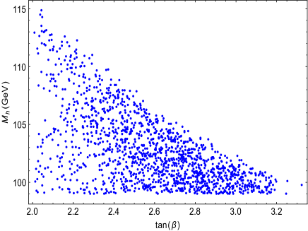
Figure 1: Tree level contribution to the Higgs-like boson mass as function of $\tan(\beta)$.

For sake of completeness, we obtain the eigenvector associated to the eigenvalue $125$ GeV for the following set of values of the parameters

$$\tan(\beta)=2.7,\,\,\,\tan(\beta_{\eta})=10,\,\,\,\tan(\beta_{\rho})=10,\,\,\,\tan(\beta_{\chi})=1.2,\,\,\,v_{\eta}=22.3\,\mathrm{GeV},\,\,\,v_{\eta^{\prime}}=223.2\,\mathrm{GeV},$$

$$v_{\rho}=8.1\,\mathrm{GeV},\,\,\,v_{\rho^{\prime}}=81\,\mathrm{GeV},\,\,\,v_{\chi}=1763.6\,\mathrm{GeV},\,\,\,v_{\chi^{\prime}}=2116.4\,\mathrm{GeV},\,\,\,f_{1}=0.01,\,\,\,f_{1}^{\prime}=0.6,$$

$$k_{1}=-500\,\mathrm{GeV},\,\,\,k_{2}=-600\,\mathrm{GeV},\,\,\,b_{\eta}=-55000\,\mathrm{GeV}^{2},\,\,\,b_{\rho}=-1.7\times 10^{6}\,\mathrm{GeV}^{2},$$

$$b_{\chi}=-1.4\times 10^{6}\,\mathrm{GeV}^{2},\mu_{\rho}=-1700\,\mathrm{GeV},\,\,\,\mu_{\eta}=-550\,\mathrm{GeV},\,\,\,\mu_{\chi}=-1400\,\mathrm{GeV}.$$ (46)

In this case, the eigenvector corresponding to the 125 GeV Higgs is

$$h=-0.93R_{\eta^{\prime}}-0.34R_{\rho^{\prime}}-0.09R_{\eta}-0.03R_{\rho}-0.05R_{\chi^{\prime}}-0.06R_{\chi}.$$ (47)

See that the eigenvector $h$ is composed mainly by $R_{\eta^{\prime}}$ and $R_{\rho^{\prime}}$. For any other choice of the set of values of the parameters, the eigenvector will keep being dominantly a composition of $R_{\eta^{\prime}}$ and $R_{\rho^{\prime}}$.

III.2 One Loop Level Contribution

In the MSSM a 125 GeV Higgs demands robust loop corrections which requires stop heavy enough such that threaten the naturalness principle. In the minimal SUSY331 model things are a little different once tree level contribution to the Higgs-like boson mass may surpass $100$ GeV.

In what follows we calculate numerically, by employing the package Spheno, the Higgs-like boson mass but taking into account one loop corrections. Our results are displayed in graphics showing the behavior of our Higgs-like boson mass with the parameters $M_{s}$, $X_{t}$ and $v_{331}$. For the other parameters, we take the values

$$\centering f_{1}=0.001\,\@add@centering f_{1}^{\prime}=0.6\,,$$ ,

$$k_{1}=-500\,\mathrm{GeV}\, k_{2}=-600\,\mathrm{GeV}\,,$$ ,

$$\mu_{\eta}=-550\,\mathrm{GeV},\,\mu_{\rho}= - 1700\,\mathrm{GeV}\,,\mu_{\chi}=-1400\,\mathrm{GeV}\,,$$

$$\tan{\beta}=2,\tan{\beta_{\eta}}= \tan{\beta_{\rho}}=10,\tan{\beta_{\chi}}=1.20\,,$$

$$A_{0},B_{0} = 1000\,\mathrm{GeV}.$$ (48)

In FIG. 2 we plot $M_{h}$ versus $X_{t}$. As we can see in that plot, small $X_{t}$ is allowed for large value of $v_{331}$, while large $X_{t}$ is allowed by small values of $v_{331}$. Moreover, observe that we may obtain a 125 GeV Higgs in the minimal SUSY331 model even for $X_{t}=0$. We highlight this result because it is not allowed in the MSSM.

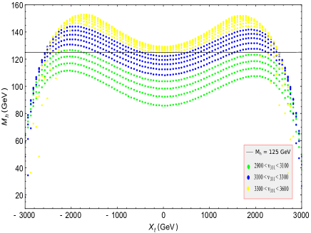
Figure 2: $M_{h}$ vs $X_{t}$ for various values of $v_{331}$. We took $m_{SUSY_{L}}=m_{SUSY_{R}}=[500,1000]$ GeV.

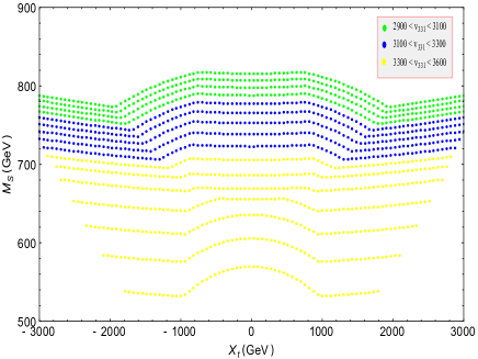
Figure 3: $M_{s}$ versus $X_{t}$ for various values of $v_{331}$.

We also obtained the $2\times 2$ mass matrix for the stops and diagonalized it with the Spheno package. The result is displayed in FIG. 3 where we show the behavior of $M_{s}$ with $X_{t}$. Note that the larger $v_{331}$, the smaller $M_{s}$. In FIG. 4 we show the behavior of $M_{h}$ with $M_{s}$ for the specific case $X_{t}=0$, and in FIG. 5 we show the behavior of $M_{h}$ with $v_{331}$ for $X_{t}=0$. Perceive that the model provides easily a $125$ GeV Higgs boson for $M_{s}$ and $X_{t}$, both, below the TeV scale.

As we can see, the minimal SUSY331 model naturally recovers the standard Higgs boson mass, but we know that it is different from the MSSM one because of the peculiarities of the minimal SUSY331 model. Thus, in order to conclude definitely that our Higgs-like boson recovers all the observed properties of the standard Higgs, we need to calculate its branching ratios and the respective signal strengths and confront the results with the experimental data measured by LHC.

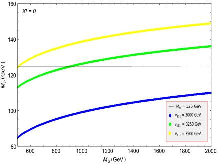
Figure 4: $M_{h}$ versus $M_{s}$ for $X_{t}=0$ for three different values of $v_{331}$.

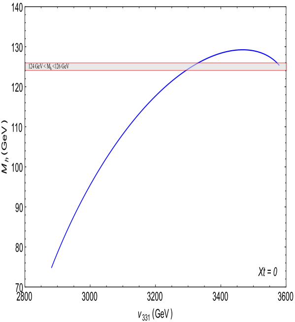
Figure 5: $M_{h}$ versus $v_{331}$ for $X_{t}=0$.

IV Branching Ratios and signal strengths

In what concerns the standard Higgs, any extension of the SM must possess a scalar with 125 GeV of mass and couplings with the standard particles that fit the measured branching ratios and signal strengths Andersen et al. (2013). This is the reason why we wonder if the Higgs-like boson discussed here recovers the Higgs branching ratios and signal strengths as observed by LHC. Our analysis is done for the following set of parameters

$$f_{1}^{\prime}=0.6\,,\,-0.03\leq f_{1}\leq 0.2\,,$$

$$k_{1}=-500\,\mathrm{GeV}\,,k_{2}=-600\,\mathrm{GeV}\,,$$

$$\mu_{\eta}=-550\,\mathrm{GeV},\,\mu_{\rho}=-1700\,\mathrm{GeV}\,,\mu_{\chi}=-1400\,\mathrm{GeV}\,,$$

$$\tan{\beta_{\eta}},\,\,\tan{\beta_{\rho}}=10,\,\tan{\beta_{\chi}}=1.20\,,$$

$$1000\,\mathrm{GeV}\leq v_{331}\leq 5000\,\mathrm{GeV}\,,\,2\leq\,\tan{\beta}\,\leq 10,$$

$$500\,\mathrm{GeV}\leq m_{SUSY_{L}},\,m_{SUSY_{R}}\leq 2000\,\mathrm{GeV},$$

$$X_{t}=0,\,\,\,A_{0},B_{0}=1000\,\mathrm{GeV}.$$ (49)

As we know, the Higgs prefers to decay into pairs of $b\bar{b}$, $WW^{*}$, $\tau\bar{\tau}$, $ZZ^{*}$ and $\gamma\gamma$. We restrict our investigation for these channels. Our results are shown in FIG. 6. Perceive that the predictions are in perfect agreement with the values measured by ATLASAad et al. (2016) and CMSCollaboration (2014). In this point of the work, we are secure in affirming that the minimal SUSY331 model is privileged in what concerns Higgs physics since it posseses a Higgs-like boson with mass and couplings with the standard particles that recovers its observed properties and respecting the naturalness principle.

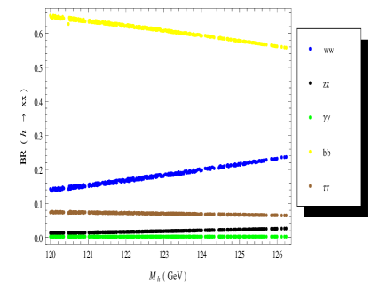
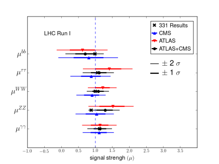
Figure 6: Left: The dominant branching ratios for our Higgs-like boson as function of its mass. Right: Decay signal strengths taking into account the combination of ATLAS and CMS data. The error bars indicate the $1\sigma$ (thick lines) and $2\sigma$ (thin lines) intervals. The combined results show a remarkable agreement with the SM prediction (normalized to $\mu=1$)

V Flavor Changing Neutral Current as Signature of our Higgs-like boson

As we saw above, the lightest Higgs of the minimal SUSY331 model fulfills the conditions to be a SM-like Higgs. However, it is important to recall that our Higgs-like bosom is different from the SM-like one in many aspects with the major one being that itintermediates flavor changing processes involving quarks already at tree level. This is a consequence of quark masses having more than one source, as depicted in the superpotential of the model. According to the last line of the superpotential, and the fact that our Higgs-like boson is mostly a composition of $R_{\eta^{\prime}}$ and $R_{\rho^{\prime}}$, the dominant flavor changing processes are those involving the third family of quarks. We studied all the possible processes here and obtained that the decays $h\rightarrow bs\,,\,bd$ are very surppressed even in relation to the loop predictions of the SMBenitez-Guzm n et al. (2015). Thus, the significant processes are those involving the Yukawa interactions $t-h-u$ and $t-h-c$. For this case, the signature of our Higgs-like boson is through top quark decays via Higgs-mediated flavor-changing processes Khachatryan et al. (2017). The behavior of the branching ratio of these decays as function of $v_{331}$ is presented in FIG. 7. Our calculations were done for the following region of the parameter space

$$f_{1}^{\prime}=0.6\,,\,-0.03\leq f_{1}\leq 0.2\,,$$

$$k_{1}=-500\,\mathrm{GeV}\,,k_{2}=-600\,\mathrm{GeV}\,,$$

$$\mu_{\eta}=-550\,\mathrm{GeV},\,\mu_{\rho}=-1700\,\mathrm{GeV}\,,\mu_{\chi}=-1400\,\mathrm{GeV}\,,$$

$$\tan{\beta_{\eta}},\,\,\tan{\beta_{\rho}}=10,\,\tan{\beta_{\chi}}=1.20\,,$$

$$2000\,\mathrm{GeV}\leq v_{331}\leq 4000\,\mathrm{GeV}\,,\,2\leq\,\tan{\beta}\,\leq 4,$$

$$800\,\mathrm{GeV}\leq m_{SUSY_{L}},\,m_{SUSY_{R}}\leq 1200\,\mathrm{GeV},$$

$$-5000\leq X_{t}\leq 5000,\,\,\,A_{0},B_{0}=1000\,\mathrm{GeV}.$$ (50)

Although our results are far below the excluded region, we hope this to be probed in the next generation of collider.

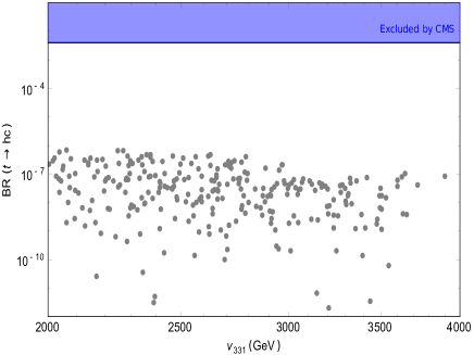
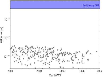
Figure 7: Calculation of the branching ratios for the top decays $t\rightarrow hc$ and $t\rightarrow hu$.

VI Stability of the potential

In this section we check if that region of parameter space considered throughout this paper is so that the potential of the model is stable for such value of the parameters. In practical terms, we have to be sure that the minimum of the potential we are considering is in fact the global one. We check this by means of the Vevacious Package Camargo-Molina et al. (2014, 2013). We export the model implemented in the Sarah package to the Vevacious one and scanned that region of the parameter space used in the results above. Our result is presented in the plane $\tan(\beta)$ versus $v_{331}$ displayed in FIG. 8 .

$$f_{1}^{\prime}=0.6\,,\,-0.03\leq f_{1}\leq 0.2\,,$$

$$k_{1}=-500\,\mathrm{GeV}\,,k_{2}=-600\,\mathrm{GeV}\,,$$

$$\mu_{\eta}=-550\,\mathrm{GeV},\,\mu_{\rho}=-1700\,\mathrm{GeV}\,,\mu_{\chi}=-1400\,\mathrm{GeV}\,,$$

$$\tan{\beta_{\eta}},\,\,\tan{\beta_{\rho}}=10,\,\tan{\beta_{\chi}}=1.20\,,$$

$$1000\,\mathrm{GeV}\leq v_{331}\leq 5000\,\mathrm{GeV}\,,\,2\leq\,\tan{\beta}\,\leq 10,$$

$$500\,\mathrm{GeV}\leq m_{SUSY_{L}},\,m_{SUSY_{R}}\leq 2000\,\mathrm{GeV},$$

$$-3000\leq X_{t}\leq 3000,\,\,\,A_{0},B_{0}=1000\,\mathrm{GeV}.$$ (51)

Perceive that, except for a small region of the parameter space presenting long lived behavior, but with decay time larger than the age of our Universe (blue region), major part of the region of the parameter space considered in this work is associated to a stable minimum of the potential.

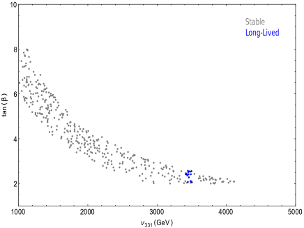
Figure 8: Points in the plane $\tan(\beta)$ versus $v_{331}$ that guarantee stability of the potential.

VII Conclusions

In this work we developed the Higgs sector of the minimal SUSY331 model with the focus on the lightest Higgs. We obtained its mass and couplings with the standard particles. With regard to its mass, tree level contribution may surpass the usual MSSM prediction and attain more than 100 GeV. Consequently, a 125 GeV Higgs will demand feeble loop corrections. In our calculations we showed that a 125 GeV Higgs is compatible with stop with mass below the TeV scale running in the loops. This is a remarkable result concerning the naturalness principle.

Although Higgs mass is the most important aspect of the Higgs physics, a complete work demands we extend our investigation to the Higgs couplings with the standard particles. We performed such an analysis and confirmed that they recover the observed pattern of branching ratios and signal strengths for its dominant processes. Finally we discussed the signature of our Higgs-like boson which manifests in the form of flavor changing processes intermediated by the Higgs. The most relevant ones are the top decay channels $t\rightarrow h+u$ and $t\rightarrow h+c$. We studied the behavior of these processes and concluded that they are out of reach of the LHC but, perhaps, may be probed in future colliders. We also checked if the region of parameter space considered in this work is compatible with the stability of the potential. We obtained that, except for a small region of the parameter space presenting long lived behavior, but with decay time larger than the age of our Universe, major part of it belongs to those points where the potential has a stable global minimum. All of this leads us to conclude that the minimal SUSY331 model is an interesting supersymmetric model for particle physics.

Appendix A

$$\left\langle\frac{\partial V}{\partial\rho^{0}}\right\rangle_{0} = (m^{2}_{\rho}+\mu_{\rho}^{2})v_{\rho}+b_{\rho}v_{\rho^{\prime}}+\frac{1}{12}g^{2}v_{\rho}\left(-v_{\eta}^{2}+v_{\eta^{\prime}}^{2}-v_{\chi}^{2}+v_{\chi^{\prime}}^{2}+2v_{\rho}^{2}-2v_{\rho^{\prime}}^{2}\right)$$

$$+ \frac{1}{2}g_{N}^{2}v_{\rho}\left(-v_{\chi}^{2}+v_{\chi^{\prime}}^{2}+v_{\rho}^{2}-v_{\rho^{\prime}}^{2}\right)+\frac{1}{\sqrt{2}}f_{1}^{\prime}\left(v_{\eta^{\prime}}v_{\chi^{\prime}}\mu_{\rho}\right)$$

$$+ \frac{1}{\sqrt{2}}f_{1}\left(\frac{1}{\sqrt{2}}v_{\eta}^{2}v_{\rho}+\frac{1}{\sqrt{2}}v_{\chi}^{2}v_{\rho}+v_{\eta}v_{\chi^{\prime}}\mu_{\chi}+v_{\eta^{\prime}}v_{\chi}\mu_{\eta}\right)+\frac{1}{\sqrt{2}}k_{1}v_{\eta}v_{\chi}=0,$$

$$\left\langle\frac{\partial V}{\partial\rho^{\prime 0}}\right\rangle_{0} = (m^{2}_{\rho^{\prime}}+\mu_{\rho}^{2})v_{\rho^{\prime}}+b_{\rho}v_{\rho}+\frac{1}{12}g^{2}v_{\rho^{\prime}}\left(v_{\eta}^{2}-v_{\eta^{\prime}}^{2}+v_{\chi}^{2}-v_{\chi^{\prime}}^{2}-2v_{\rho}^{2}+2v_{\rho^{\prime}}^{2}\right)$$

$$+ \frac{1}{2}g_{N}^{2}v_{\rho^{\prime}}\left(-v_{\chi}^{2}+v_{\chi^{\prime}}^{2}+v_{\rho}^{2}-v_{\rho^{\prime}}^{2}\right)+\frac{1}{\sqrt{2}}f_{1}\left(v_{\eta}v_{\chi}\mu_{\rho}\right)$$

$$+ \frac{1}{\sqrt{2}}f_{1}^{\prime}\left(\frac{1}{\sqrt{2}}v_{\eta^{\prime}}^{2}v_{\rho^{\prime}}+\frac{1}{\sqrt{2}}v_{\chi^{\prime}}^{2}v_{\rho^{\prime}}+v_{\eta}v_{\chi^{\prime}}\mu_{\eta}+v_{\eta^{\prime}}v_{\chi}\mu_{\chi}\right)+\frac{1}{\sqrt{2}}k_{2}v_{\eta^{\prime}}v_{\chi^{\prime}}=0,$$

$$\left\langle\frac{\partial V}{\partial\eta^{0}}\right\rangle_{0} = (m^{2}_{\eta}+\mu_{\eta}^{2})v_{\eta}+b_{\eta}v_{\eta^{\prime}}+\frac{1}{12}g^{2}v_{\eta}\left(-v_{\rho}^{2}+v_{\rho^{\prime}}^{2}-v_{\chi}^{2}+v_{\chi^{\prime}}^{2}+2v_{\eta}^{2}-2v_{\eta^{\prime}}^{2}\right)$$

$$+ \frac{1}{2}f_{1}^{\prime}\left(v_{\rho^{\prime}}v_{\chi^{\prime}}\mu_{\eta}\right)+\frac{1}{\sqrt{2}}f_{1}\left(\frac{1}{\sqrt{2}}v_{\rho}^{2}v_{\eta}+\frac{1}{\sqrt{2}}v_{\chi}^{2}v_{\eta}+v_{\rho}v_{\chi^{\prime}}\mu_{\chi}+v_{\rho^{\prime}}v_{\chi}\mu_{\rho}\right)$$

$$+ \frac{1}{\sqrt{2}}k_{1}v_{\rho}v_{\chi}=0,$$

$$\left\langle\frac{\partial V}{\partial\eta^{\prime 0}}\right\rangle_{0} = (m^{2}_{\eta^{\prime}}+\mu_{\eta}^{2})v_{\eta^{\prime}}+b_{\eta}v_{\eta}+\frac{1}{12}g^{2}v_{\eta^{\prime}}\left(v_{\rho}^{2}-v_{\rho^{\prime}}^{2}+v_{\chi}^{2}-v_{\chi^{\prime}}^{2}-2v_{\eta}^{2}+2v_{\eta^{\prime}}^{2}\right)$$

$$+ \frac{1}{\sqrt{2}}f_{1}\left(v_{\rho}v_{\chi}\mu_{\eta}\right)+\frac{1}{\sqrt{2}}f_{1}^{\prime}\left(\frac{1}{\sqrt{2}}v_{\rho^{\prime}}^{2}v_{\eta^{\prime}}+\frac{1}{\sqrt{2}}v_{\chi^{\prime}}^{2}v_{\eta^{\prime}}+v_{\rho}v_{\chi^{\prime}}\mu_{\rho}+v_{\rho^{\prime}}v_{\chi}\mu_{\chi}\right)$$

$$+ \frac{1}{\sqrt{2}}k_{2}v_{\rho^{\prime}}v_{\chi^{\prime}}=0,$$

$$\left\langle\frac{\partial V}{\partial\chi^{0}}\right\rangle_{0} = (m^{2}_{\chi}+\mu_{\chi}^{2})v_{\chi}+b_{\chi}v_{\chi^{\prime}}+\frac{1}{12}g^{2}v_{\chi}\left(-v_{\eta}^{2}+v_{\eta^{\prime}}^{2}-v_{\rho}^{2}+v_{\rho^{\prime}}^{2}+2v_{\chi}^{2}-2v_{\chi^{\prime}}^{2}\right)$$

$$+ \frac{1}{2}g_{N}^{2}v_{\chi}\left(v_{\chi}^{2}-v_{\chi^{\prime}}^{2}-v_{\rho}^{2}+v_{\rho^{\prime}}^{2}\right)+\frac{1}{\sqrt{2}}f_{1}^{\prime}\left(v_{\eta^{\prime}}v_{\rho^{\prime}}\mu_{\chi}\right)$$

$$+ \frac{1}{\sqrt{2}}f_{1}\left(\frac{1}{\sqrt{2}}v_{\eta}^{2}v_{\chi}+\frac{1}{\sqrt{2}}v_{\rho}^{2}v_{\chi}+v_{\eta}v_{\rho^{\prime}}\mu_{\rho}+v_{\eta^{\prime}}v_{\rho}\mu_{\eta}\right)+\frac{1}{\sqrt{2}}k_{1}v_{\eta}v_{\rho}=0,$$

$$\left\langle\frac{\partial V}{\partial\chi^{\prime 0}}\right\rangle_{0} = (m^{2}_{\chi^{\prime}}+\mu_{\chi^{\prime}}^{2})v_{\chi^{\prime}}+b_{\chi}v_{\chi}+\frac{1}{12}g^{2}v_{\chi^{\prime}}\left(v_{\eta}^{2}-v_{\eta^{\prime}}^{2}+v_{\rho}^{2}-v_{\rho^{\prime}}^{2}-2v_{\chi}^{2}+2v_{\chi^{\prime}}^{2}\right)$$ (52)

$$+ \frac{1}{2}g_{N}^{2}v_{\chi^{\prime}}\left(-v_{\chi}^{2}+v_{\chi^{\prime}}^{2}+v_{\rho}^{2}-v_{\rho^{\prime}}^{2}\right)+\frac{1}{\sqrt{2}}f_{1}\left(v_{\eta}v_{\rho}\mu_{\chi}\right)$$

$$+ \frac{1}{\sqrt{2}}f_{1}^{\prime}\left(\frac{1}{\sqrt{2}}v_{\eta^{\prime}}^{2}v_{\chi^{\prime}}+\frac{1}{\sqrt{2}}v_{\rho^{\prime}}^{2}v_{\chi^{\prime}}+v_{\eta}v_{\rho^{\prime}}\mu_{\eta}+v_{\eta^{\prime}}v_{\rho}\mu_{\rho}\right)+\frac{1}{\sqrt{2}}k_{2}v_{\eta^{\prime}}v_{\rho^{\prime}}=0.$$

References

• Aad et al. (2012) G. Aad et al. (ATLAS), Phys. Lett., B716, 1 (2012), arXiv:1207.7214 [hep-ex] .
• Chatrchyan et al. (2012) S. Chatrchyan et al. (CMS), Phys. Lett., B716, 30 (2012), arXiv:1207.7235 [hep-ex] .
• Aad et al. (2016) G. Aad et al. (ATLAS, CMS), JHEP, 08, 045 (2016a), arXiv:1606.02266 [hep-ex] .
• Carena and Haber (2003) M. Carena and H. E. Haber, Prog. Part. Nucl. Phys., 50, 63 (2003), arXiv:hep-ph/0208209 [hep-ph] .
• Pisano and Pleitez (1992) F. Pisano and V. Pleitez, Phys. Rev., D46, 410 (1992), arXiv:hep-ph/9206242 [hep-ph] .
• Frampton (1992) P. H. Frampton, Phys. Rev. Lett., 69, 2889 (1992).
• Montero et al. (2002) J. C. Montero, C. A. de S. Pires,  and V. Pleitez, Phys. Rev., D66, 113003 (2002a), arXiv:hep-ph/0112203 [hep-ph] .
• Queiroz et al. (2010) F. Queiroz, C. A. de S. Pires,  and P. S. R. da Silva, Phys. Rev., D82, 065018 (2010), arXiv:1003.1270 [hep-ph] .
• Dong and Si (2014) P. V. Dong and D. T. Si, Phys. Rev., D90, 117703 (2014), arXiv:1411.4400 [hep-ph] .
• de Sousa Pires and Ravinez (1998) C. A. de Sousa Pires and O. P. Ravinez, Phys. Rev., D58, 035008 (1998), [Phys. Rev.D58,35008(1998)], arXiv:hep-ph/9803409 [hep-ph] .
• de Sousa Pires (1999) C. A. de Sousa Pires, Phys. Rev., D60, 075013 (1999), arXiv:hep-ph/9902406 [hep-ph] .
• Pal (1995) P. B. Pal, Phys. Rev., D52, 1659 (1995), arXiv:hep-ph/9411406 [hep-ph] .
• Dias and Pleitez (2004) A. G. Dias and V. Pleitez, Phys. Rev., D69, 077702 (2004), arXiv:hep-ph/0308037 [hep-ph] .
• Dias et al. (2003) A. G. Dias, C. A. de S. Pires,  and P. S. Rodrigues da Silva, Phys. Rev., D68, 115009 (2003), arXiv:hep-ph/0309058 [hep-ph] .
• Ferreira et al. (2017) J. G. Ferreira, C. A. de S. Pires, J. G. Rodrigues,  and P. S. Rodrigues da Silva, Phys. Lett., B771, 199 (2017), arXiv:1612.01463 [hep-ph] .
• Duong and Ma (1993) T. V. Duong and E. Ma, Phys. Lett., B316, 307 (1993), arXiv:hep-ph/9306264 [hep-ph] .
• Montero et al. (2002) J. C. Montero, V. Pleitez,  and M. C. Rodriguez, Phys. Rev., D65, 035006 (2002b), arXiv:hep-ph/0012178 [hep-ph] .
• Huong et al. (2013) D. T. Huong, L. T. Hue, M. C. Rodriguez,  and H. N. Long, Nucl. Phys., B870, 293 (2013), arXiv:1210.6776 [hep-ph] .
• Ferreira et al. (2013) J. G. Ferreira, C. A. de S. Pires, P. S. Rodrigues da Silva,  and A. Sampieri, Phys. Rev., D88, 105013 (2013), arXiv:1308.0575 [hep-ph] .
• Staub (2008) F. Staub,  (2008), arXiv:0806.0538 [hep-ph] .
• Staub (2015) F. Staub, Adv. High Energy Phys., 2015, 840780 (2015), arXiv:1503.04200 [hep-ph] .
• Vicente (2015) A. Vicente,  (2015), arXiv:1507.06349 [hep-ph] .
• Porod (2003) W. Porod, Comput. Phys. Commun., 153, 275 (2003), arXiv:hep-ph/0301101 [hep-ph] .
• Porod and Staub (2012) W. Porod and F. Staub, Comput. Phys. Commun., 183, 2458 (2012), arXiv:1104.1573 [hep-ph] .
• Staub et al. (2012) F. Staub, T. Ohl, W. Porod,  and C. Speckner, Comput. Phys. Commun., 183, 2165 (2012), arXiv:1109.5147 [hep-ph] .
• Andersen et al. (2013) J. R. Andersen et al. (LHC Higgs Cross Section Working Group),  (2013), doi:10.5170/CERN-2013-004arXiv:1307.1347 [hep-ph] .
• Aad et al. (2016) G. Aad et al. (ATLAS), Eur. Phys. J., C76, 6 (2016b), arXiv:1507.04548 [hep-ex] .
• Collaboration (2014) C. Collaboration (CMS),  (2014).
• Benitez-Guzm n et al. (2015) L. G. Benitez-Guzm n, I. Garc a-Jim nez, M. A. L pez-Osorio, E. Mart nez-Pascual,  and J. J. Toscano, J. Phys., G42, 085002 (2015), arXiv:1506.02718 [hep-ph] .
• Khachatryan et al. (2017) V. Khachatryan et al. (CMS), JHEP, 02, 079 (2017), arXiv:1610.04857 [hep-ex] .
• Camargo-Molina et al. (2014) J. E. Camargo-Molina, B. Garbrecht, B. O’Leary, W. Porod,  and F. Staub, Phys. Lett., B737, 156 (2014), arXiv:1405.7376 [hep-ph] .
• Camargo-Molina et al. (2013) J. E. Camargo-Molina, B. O’Leary, W. Porod,  and F. Staub, Eur. Phys. J., C73, 2588 (2013), arXiv:1307.1477 [hep-ph] .