Phase Transitions between Different Spin-Glass Phases and
between Different Chaoses in Quenched Random Chiral Systems

Abstract

The left-right chiral and ferromagnetic-antiferromagnetic double spin-glass clock model, with the crucially even number of states $q=4$ and in three dimensions $d=3$, has been studied by renormalization-group theory. We find, for the first time to our knowledge, four different spin-glass phases, including conventional, chiral, and quadrupolar spin-glass phases, and phase transitions between spin-glass phases. The chaoses, in the different spin-glass phases and in the phase transitions of the spin-glass phases with the other spin-glass phases, with the non-spin-glass ordered phases, and with the disordered phase, are determined and quantified by Lyapunov exponents. It is seen that the chiral spin-glass phase is the most chaotic spin-glass phase. The calculated phase diagram is also otherwise very rich, including regular and temperature-inverted devil’s staircases and reentrances.

I Introduction

Spin-glass phases, created by competing frustrated random ferromagnetic and antiferromagnetic interactions, have been known NishimoriBook to incorporate a plethora of interesting complex phenomena, not the least being the natural generation chaos McKayChaos ; McKayChaos2 ; BerkerMcKay . Recently, it has been shown Caglar ; Caglar2 that competing left- and right-chiral interactions also create spin-glass phases, even in the absence of competing ferromagnetic and antiferromagnetic interactions. First shown Caglar with chiral Potts models Ostlund ; Kardar ; Huse ; Huse2 ; Caflisch with the inclusion of quenched randomness, chiral spin glasses were recently extended Caglar2 to clock models with an odd number of states $(q=5)$, resulting in a literally moviesque sequence of phase diagrams, including regular and inverted devil’s staircases, a chiral spin-glass phase, and algebraic order.

The chiral clock model work was purposefully initiated Caglar2 with odd number of states $q$, in order to deal with the complexity of the global phase diagram, since it is known that the odd $q$ models do not show Ilker3 the traditional ferromagnetic-antiferromagnetic spin-glass phase. This is because neighboring, antiferromagnetically interacting odd $q$ clock spins cannot achieve perfect antiferromagnetic alignment. Furthermore, there are two configurations for the near-antiferromagnetic alignment, creating a built-in disorder. The traditional ferromagnetic-antiferromagnetic spin-glass phase does not occur and the antiferromagnetic phase is a critical phase lacking conventional long-range order.Ilker3 On the other hand, the even $q$ clock spins can achieve complete antiferromagnetic pairing, and exhibit the conventional antiferromagnetic long-range order and the traditional ferromagnetic-antiferromagnetic spin-glass phase.Ilker1 Thus, the current study is on the random chiral clock model with an even number of states $(q=4)$, which supports the ferromagnetic-antiferromagnetic usual spin-glass phase Ilker1 , as well as, as we shall see below, with added phase diagram complexity, the chiral spin-glass phase and two other new spin-glass phases. A double spin-glass model is constructed, including competing quenched random left-right chiral and ferromagnetic-antiferromagnetic interactions, and solved in three dimensions by renormalization-group theory.

The extremely rich phase diagram includes, to our knowledge for the first time, more than one (four) spin-glass phases on the same phase diagram and three separate spin-glass-to-spin-glass phase transitions. These constitute phase transitions between chaoses. We determine the chaotic behaviors of the spin-glass phases, of the phase transitions between the spin-glass phases, of the phase transitions between the spin-glass phases and the ferromagnetic, antiferromagnetic, quadrupolar, and disordered phases.

II Doubly Spin Glass System:
Left-Right Chiral and Ferro-Antiferro Interactions

The $q-$state clock spin glass is composed of unit spins that are confined to a plane and that can only point along $q$ angularly equidistant directions, with Hamiltonian

$$-\beta{\cal H}=\sum_{\left<ij\right>}J_{ij}\vec{s}_{i}.\vec{s}_{j}=\sum_{\left<ij\right>}J_{ij}\cos\theta_{ij},$$ (1)

where $\beta=1/k_{B}T$, $\theta_{ij}=\theta_{i}-\theta_{j}$, at each site $i$ the spin angle $\theta_{i}$ takes on the values $(2\pi/q)\sigma_{i}$ with $\sigma_{i}=0,1,2,\ldots,(q-1)$, and $\left<ij\right>$ denotes summation over all nearest-neighbor pairs of sites. As the long-studied ferromagnetic-antiferromagnetic spin-glass system NishimoriBook , the bond strengths $J_{ij}$, with quenched (frozen) ferromagnetic-antiferromagnetic randomness, are $+J>0$ (ferromagnetic) with probability $1-p$ and $-J$ (antiferromagnetic) with probability $p$, with $0\leq p\leq 1$. Thus, the ferromagnetic and antiferromagnetic interactions locally compete in frustration centers. Recent studies on ferromagnetic-antiferromagnetic clock spin glasses are in Refs. Ilker1 ; Ilker3 ; Lupo .

In the $q-$state chiral clock double spin glass, recently introduced (and used in the qualitatively different odd $q=5$), frustration also occurs via randomly frozen left or right chirality Caglar , thus doubling the spin-glass mechanisms. The Hamiltonian in Eq. (1) is generalized to random local chirality,

$$-\beta{\cal H}=\sum_{\left<ij\right>}[J_{ij}\cos\theta_{ij}+\Delta\,\delta(\theta_{ij}+\eta_{ij}\frac{2\pi}{q})].$$ (2)

In a cubic lattice, as sites along the respective coordinate directions are considered, the $x,y,$ or $z$ coordinates increase. Since bond moving in the Migdal-Kadanoff approximation Migdal ; Kadanoff is done transversely to the bond directions, this sequencing is respected. Equivalently, in the corresponding hierarchical lattice BerkerOstlund ; Kaufman1 ; Kaufman2 ; McKay ; Hinczewski1 , one can always define a direction along the connectivity, for example from left to right, and assign consecutive increasing number labels to the sites. In Eq. (2), for each pair of nearest-neighbor sites $\left<ij\right>$ the numerical site label $j$ is ahead of $i$, frozen (quenched) $\eta_{ij}=1$ (left chirality) or $-1$ (right chirality), and the delta function $\delta(x)=1\,(0)$ for $x=0\,(x\neq 0)$. The overall concentrations of left and right chirality are respectively $1-c$ and $c$, with $0\leq c\leq 1$. The strength of the random chiral interaction is $\Delta/J$, with temperature divided out. Thus, the system is chiral for $\Delta\neq 0$, chiral-symmetric for $c=0.5$, chiral-symmetry-broken for $c\neq 0.5$. The global phase diagram is in terms of temperature $J^{-1}$, antiferromagnetic bond concentration $p$, random chirality strength $\Delta/J$, and chiral symmetry-breaking concentration $c$.

III Renormalization-Group Method: Migdal-Kadanoff Approximation and Exact Hierarchical Lattice Solution

Our method, previously described in extensive detail Caglar2 and used on a qualitatively different model with qualitatively different results, is simultaneously the Migdal-Kadanoff approximation Migdal ; Kadanoff for the cubic lattice and the exact solution BerkerOstlund ; Kaufman1 ; Kaufman2 ; McKay ; Hinczewski1 for a $d=3$ hierarchical lattice, with length rescaling factor $b=3$. Exact calculations on hierarchical lattices are also currently widely used on a variety of statistical mechanics Derrida ; Thorpe ; Efrat ; Monthus2 ; Lyra ; Xu2014 ; Silva ; Boettcher1 ; Boettcher2 ; Hirose2 ; Boettcher3 ; Nandy ; Boettcher4 ; Bleher ; Zhang2017 , finance Sirca , and, most recently, DNA-binding Maji problems.

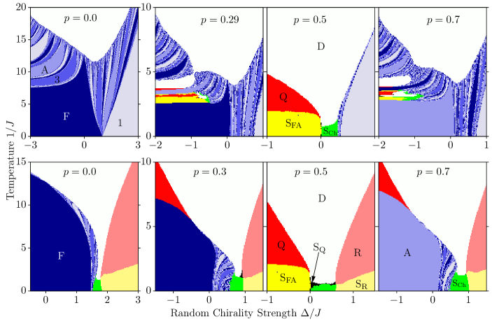
Figure 1: (Color online) A calculated sequence of phase diagrams for the left chiral ($c=0$), on the upper side, and quenched random left and right chiral ($c=0.5$), on the lower side, systems with, in both cases, quenched random ferromagnetic and antiferromagnetic interactions. The horizontal axis is the random chirality strength $\Delta/J$. The consecutive phase diagrams are for different concentrations $p$ of antiferromagnetic interactions. The system exhibits a ferromagnetic phase F, an antiferromagnetic phase A, a multitude of different chiral phases, a quadrupolar phases Q, a ”one-step” phase R, and four differently ordered spin-glass phases: the chiral spin-glass S_CH, the usual ferromagnetic-antiferromagnetic spin glass S_FA, the quadrupolar spin glass S_Q, and S_R. The phase diagrams obtained from $p$ and $1-p$ are symmetric, since the system has an even number of spin directions. On some of the chiral phases, the $\pi/2$ multiplicity of the asymptotically dominant interaction is indicated. The ferromagnetic and chiral phases accumulate as different devil’s staircases at their boundary with the disordered (D) phase.

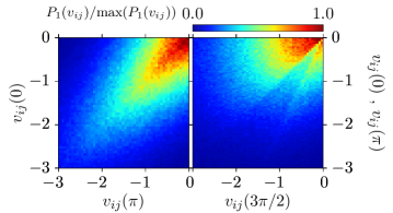
Figure 2: (Color online) Asymptotic fixed distribution of the chiral spin-glass phase S_Ch. The part of the fixed distribution $P_{1}({\bf V}_{ij})$, for the interactions ${\bf V}_{ij}$ in which $V_{ij}(\pi/2)$ is maximum and therefore $0$ (and the other three interactions are negative) is shown in this figure, with $v_{ij}(\theta)=V_{ij}(\theta)/\left<\left|V_{ij}(\theta)\right|\right>$. The projections of $P_{1}({\bf V}_{ij})$ onto two of its three arguments are shown in each panel of this figure. The other three $P_{\sigma}({\bf V}_{ij})$ have the same fixed distribution. Thus chirality is broken locally but not globally, just as, in the long-time studied ferromagnetic-antiferromagnetic spin glasses, spin-direction symmetry breaking is local but not global (i.e., the local magnetization is non-zero, the global magnetization is zero).

Figure 3: Asymptotic fixed distributions of 3 different spin-glass phases, with $v_{ij}(\theta)=V_{ij}(\theta)/\left<\left|V_{ij}(\theta)\right|\right>$. For the ferromagnetic-antiferromagnetic spin-glass S_FA phase, $r=0,\sigma=2$ and $r=2,\sigma=0$. The other two angles do not occur. For the quadrupolar spin-glass S_Q phase, $r=0,\sigma=1$ and $r=1,\sigma=0$, with $V_{ij}(0)=V_{ij}(\pi)$ and $V_{ij}(\pi/2)=V_{ij}(3\pi/2)$. For the spin-glass S_R phase, $r=1,\sigma=3$ and $r=3,\sigma=1$. The other two angles do not occur. The $v_{ij}(0)=v_{ij}(\pi)$ curve obtained from the left panel of Fig. 2 also matches the curve here.

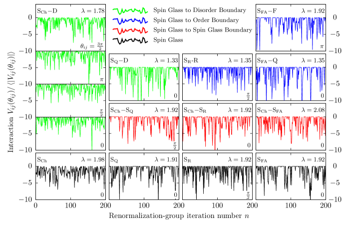
Figure 4: Chaotic renormalization-group trajectories of the four different spin-glass phases (black), of the phase boundaries of the spin-glass phases with other spin-glass phases (red), with non-spin-glass ordered (blue) and disordered (green) phases. The phase boundary chaoses of each spin-glass phase are given in their corresponding vertically aligned panels. In each case, only one of the four interactions $V_{ij}(0),V_{ij}(\pi/2),V_{ij}(\pi),V_{ij}(3\pi/2)$ at a given location $\left<ij\right>$, under consecutive renormalization-group transformations, is shown, except, for illustration, all four interactions are shown for the chaos at the phase transition between the chiral spin-glass and disordered phases. The $\theta_{ij}$ angular value of each interaction $V_{ij}(\theta_{ij})$ is indicated in the figure panels, as well as the Lyapunov exponent $\lambda$ calculated from the chaotic sequence under renormalization-group transformations. The Lyapunov exponent is calculated over 1,000 renormalization-group iterations, after throwing out the first 200 iterations. Inside all four spin-glass phases, the average interaction diverges as $<|V|>\sim b^{y_{R}n}$, where $n$ is the number of renormalization-group iterations and $y_{R}=0.25$ is the runaway exponent. At the S${}_{Ch}-$S_R, S${}_{Ch}-$S_Q, S${}_{FA}-$A, S${}_{FA}-$F phase boundaries, $y_{R}=0.25$ also. At the S${}_{Ch}-$S_FA phase boundary, $y_{R}=0.11$ for $V_{ij}(0),V_{ij}(\pi)$ and $y_{R}=0.25$ for $V_{ij}(\pi/2),V_{ij}(3\pi/2)$. At the phase boundaries of the spin-glass phases with some non-spin-glass-ordered and disordered phases, the average interaction remains non-divergent, fixed at $<V>=-0.34$ for S${}_{FA}-$Q, S${}_{R}-$R, S${}_{Q}-$D and $<V>=-1.07$ for S${}_{Ch}-$D. As indicated by the Lyapunov exponents, chaos is stronger inside the chiral spin-glass phase.

Under the renormalization-group transformation Caglar2 , the Hamiltonian of Eq. (2) maps onto the more general form

$$-\beta{\cal H}=\sum_{\left<ij\right>}V_{ij}(\theta_{ij}),$$ (3)

where $\theta_{ij}=\theta_{i}-\theta_{j}$ can take $q=4$ different values, so that for each pair $<ij>$ of nearest-neighbor sites, there are q = 4 different interaction constants

$$\{V_{ij}(\theta_{ij})\}=\\ \{V_{ij}(0),V_{ij}(\pi/2),V_{ij}(\pi),V_{ij}(3\pi/2)\}\equiv\textbf{V}_{ij},$$ (4)

which are in general different at each locality (quenched randomness). The largest element of $\{V_{ij}(\theta_{ij})\}$ at each locality $<ij>$ is set to zero, by subtracting the same constant from all $q=4$ interaction constants, with no effect on the physics; thus, the $q-1=3$ other interaction constants are negative.

The starting double-bimodal quenched probability distribution of the interactions, characterized by $p$ and $c$ as described above, is not conserved under rescaling. The renormalized quenched probability distribution of the interactions is obtained by the convolution Andelman

$$P^{\prime}(\textbf{V}^{\prime}_{i^{\prime}j^{\prime}})=\int{\left\{\prod_{ij}^{i^{\prime}j^{\prime}}d\textbf{V}_{ij}P(\textbf{V}_{ij})\right\}\delta(\textbf{V}^{\prime}_{i^{\prime}j^{\prime}}-\textbf{R}(\left\{\textbf{V}_{ij}\right\}))},$$ (5)

where $\textbf{V}_{ij}\equiv\{V_{ij}(\theta_{ij})\}$ as in Eq. (4), $\textbf{R}(\{\textbf{V}_{ij}\})$ represents the renormalization-group recursion relation Caglar2 , primes refer to the renormalized system, and the procedure is effected numerically. The different phases and phase transitions of the system are identified by the different asymptotic renormalization-group flows of the quenched probability distribution $P(\textbf{V}_{ij})$. Similar previous studies, on other spin-glass systems, are in Refs. Gingras1 ; Migliorini ; Gingras2 ; Heisenberg ; Guven ; Ohzeki ; Ilker1 ; Ilker2 ; Ilker3 ; Demirtas .

IV Global Phase Diagram:
Multiple Spin-Glass Phases

Figs. 1 show a calculated sequence of phase diagram cross sections for the left-chiral $(c=0)$, on the upper side, and quenched random left- and right-chiral $(c=0.5)$, on the lower side, systems with in both cases quenched random ferromagnetic and antiferromagnetic interactions. The system exhibits a disordered phase (D), a ferromagnetic phase (F), a conventionally ordered (in contrast to the algebraically ordered for $q=5$) antiferromagnetic phase (A), a quadrupolar phase (Q), a new ”one-step” phase (R), a multitude of different chiral phases, and four different spin-glass phases (S_Ch, S_FA, S_Q, S_R) including spin-glass-to-spin-glass phase transitions. The ferromagnetic and different chiral phases accumulate as conventional and temperature-inverted (abutting to the reentrant Cladis ; Hardouin ; Garland ; Netz ; Kumari disordered phase) devil’s staircases Bak ; Fukuda at their boundary with the disordered (D) phase. This accumulation and its multiplicity of intervening phases occur at all scales of phase diagram space (i.e., at all magnifications of the phase diagram figure, as for example seen up to 100-fold calculated magnification in Fig. 4 of Caglar2 ), which is the definition of a devil’s staircase.

Unlike the odd $q$ case of $q=5$, which incorporates built-in entropy Caglar2 even without any quenched randomness, no algebraically ordered phase BerkerKadanoff1 ; BerkerKadanoff2 occurs in this even $q$ case of $q=4$. The devil’s staircases of the chiral phases is again seen. Most interestingly, quadrupolar and ”one-step” phases, different spin-glass phases for the first time in the same phase diagram, and spin-glass-to-spin-glass direct phase transitions are seen. The phases and phase boundaries involving spin glassiness are tracked through the calculated Lyapunov exponents of their chaos.

In all ordered phases, the renormalization-group trajectories flow to strong (infinite) coupling. In the ferromagnetic phase, under renormalization-group transformations, the interaction $V_{ij}(0)$ becomes asymptotically dominant. In the antiferromagnetic phase, under renormalization-group transformations, the interaction $V_{ij}(\pi)$ becomes asymptotically dominant. In the quadrupolar phase Q, the interactions $V_{ij}(0)$ and $V_{ij}(\pi)$ become asymptotically dominant and equal. Thus, there are two such quadrupolar phases, namely along the spin directions $\pm x$ and $\pm y$, with the additional (factorized) trivial degeneracy of $\pm$ spin direction at each site. In the new ”one-step phase” R, the interactions $V_{ij}(+\pi/2)$ and $V_{ij}(-\pi/2)$ become asymptotically dominant and equal. Thus, in such a phase, the average local spins can span all spin directions, taking $\pm\pi/2$ steps from one spin to the next in the renormalized systems. The identification of the distinct chiral phases, each with distinct chiral pitches, has been explained in Ref. Caglar2 .

The renormalization-group trajectories starting in the spin-glass phases, unlike those in the ferromagnetic, antiferromagneric, quadrupolar, ”one-step”, and chiral phases, do not have the asymptotic behavior where at any scale one potential $V(\theta)$ is dominant. These trajectories of the spin-glass phases asymptotically go to a strong-coupling fixed probability distribution $P(\textbf{V}_{ij})$ which assigns non-zero probabilities to a distribution of $\textbf{V}_{ij}$ values, with no single $V_{ij}(\theta)$ being dominant. These distributions are shown in Figs. 2 and 3. Different asymptotic fixed probability distributions indicate different spin-glass phases.

Since, at each locality, the largest interaction in $\{V_{ij}(0),V_{ij}(\pi/2),V_{ij}(\pi),V_{ij}(3\pi/2)\}$ is set to zero and the three other interactions are thus made negative, by subtracting the same constant from all four interactions without affecting the physics, the quenched probability distribution $P(\textbf{V}_{ij})$, a function of four variables, is actually composed of four functions $P_{\sigma}(\textbf{V}_{ij})$ of three variables, each such function corresponding to one of the interactions being zero and the other three, arguments of the function, being negative. Figs. 2 and 3 show the latter functions.

In Fig. 2 for the spin-glass phase S_Ch, the part of the fixed distribution, $P_{1}(\textbf{V}_{ij})$, for the interactions $\textbf{V}_{ij}$ in which $V_{ij}(\pi/2)$ is maximum and therefore 0 (and the other three interactions are negative) is shown. The projections of $P_{1}(\textbf{V}_{ij})$ onto two of its three arguments are shown in each panel of Fig. 2. The other three $P_{\sigma}(\textbf{V}_{ij})$ have the same fixed distribution. Thus, chirality is broken locally, but not globally, just as, in the long-time studied ferromagnetic-antiferromagnetic spin glasses, spin-direction symmetry breaking is local but not global (i.e., the local magnetization is non-zero, the global magnetization is zero). The asymptotic fixed distribution of the phase S_Ch, given in Fig. 2, assigns non-zero probabilities to a continuum of values for all four interactions $\{V_{ij}(0),V_{ij}(\pi/2),V_{ij}(\pi),V_{ij}(3\pi/2)\}$. The phase S_Ch is therefore a chiral spin-glass phase. The similar chiral spin-glass phase has been seen previously, but as the sole spin-glass phase, for the odd $q=5$.Caglar2 . The chiral spin-glass phase occurs even when there is no competing ferromagnetic-antiferromagnetic interactions.Caglar2 ; Caglar

As seen in Fig. 3, in the asymptotic fixed distribution of the spin-glass phase S_FA, non-zero probabilities are assigned to a continuum of values of $\{V_{ij}(0),V_{ij}(\pi)\}$. Fig. 3 shows the fixed distribution values $P_{0}(V_{ij}(\pi))$ for $V_{ij}(0)$ maximum and therefore set to zero. Completing the asymptotic fixed distribution of S_FA is an identical function $P_{2}(V_{ij}(0))$ for $V_{ij}(\pi)$ maximum and therefore set to zero. At this fixed distribution, the values of $V_{ij}(\pi/2)$ and $V_{ij}(3\pi/2)$ diverge to negative infinity, so that these angles do not occur. Thus, S_FA is the long-studied NishimoriBook spin-glass phase of competing ferromagnetic and antiferromagnetic interactions.

Fig. 3 also shows the asymptotic fixed distribution of the spin-glass phase S_R, with the functions $P_{1}(V_{ij}(3\pi/2))$ for $V_{ij}(\pi/2)$ maximum (and therefore set to zero) and $P_{3}(V_{ij}(\pi/2))$ for $V_{ij}(3\pi/2)$ maximum (and therefore set to zero). Again, the other two angles do not occur at this asymptotic fixed distribution. Furthermore, Fig. 3 also shows the asymptotic fixed distribution of the spin-glass phase S_Q, with the functions $P_{0}(V_{ij}(\pi/2))$ and $P_{1}(V_{ij}(0))$, with $V_{ij}(0)=V_{ij}(\pi)$ and $V_{ij}(\pi/2)=V_{ij}(3\pi/2)$. Thus, this fixed distribution does not locally distinguish between $\pm$ spin directions and is thus a quadrupolar spin-glass phase.

In fact, the $v_{ij}(0)=v_{ij}(p)$ curve obtained from the left panel of Fig. 2 also matches the curve here. The three fixed distributions given in Fig. 3 exhibit the same numerical curve, but refer to widely different interactions. Thus, they underpin different spin-glass phases.

V Phase Transitions between Chaos

Another distinctive mechanism, that of chaos under scale change McKayChaos ; McKayChaos2 ; BerkerMcKay or, equivalently Ilker1 , chaos under spatial translation, occurs within the spin-glass phase and differently at the spin-glass phase boundary Ilker1 , in systems with competing ferromagnetic and antiferromagnetic interactions McKayChaos ; McKayChaos2 ; BerkerMcKay ; Bray ; Hartford ; Nifle1 ; Nifle2 ; Banavar ; Frzakala1 ; Frzakala2 ; Sasaki ; Lukic ; Ledoussal ; Rizzo ; Katzgraber ; Yoshino ; Pixley ; Aspelmeier1 ; Aspelmeier2 ; Mora ; Aral ; Chen ; Jorg ; Lima ; Katzgraber2 ; MMayor ; ZZhu ; Katzgraber3 ; Fernandez ; Ilker1 ; Ilker2 ; MMayor2 and, more recently, with competing left- and right-chiral interactions Caglar ; Caglar2 . Originally found in hierarchical systems McKayChaos ; McKayChaos2 ; BerkerMcKay , scaling or equivalently translation spin-glass chaos is now well accepted for real $d=3$ lattices and experimental systems McKayChaos ; McKayChaos2 ; BerkerMcKay ; Bray ; Hartford ; Nifle1 ; Nifle2 ; Banavar ; Frzakala1 ; Frzakala2 ; Sasaki ; Lukic ; Ledoussal ; Rizzo ; Katzgraber ; Yoshino ; Pixley ; Aspelmeier1 ; Aspelmeier2 ; Mora ; Aral ; Chen ; Jorg ; Lima ; Katzgraber2 ; MMayor ; ZZhu ; Katzgraber3 ; Fernandez ; Ilker1 ; Ilker2 ; MMayor2 .

Fig. 4 gives the asymptotic chaotic renormalization-group trajectories of the four different spin-glass phases and of the phase boundaries between the spin-glass phases with other spin-glass phases, with the non-spin-glass ordered phases and the disordered phase.

Chaos is measured by the Lyapunov exponent, whose calculation for the multiinteraction $V_{ij}(0),V_{ij}(\pi/),V_{ij}(\pi),V_{ij}(3\pi/2)$ case is given in Ref. Caglar2 . Spin-glass chaos occurs for $\lambda>0$ Aral and the more positive $\lambda$, the stronger is chaos. Inside all four spin-glass phases, the average interaction diverges as $<|V|>\sim b^{y_{R}n}$, where $n$ is the number of renormalization-group iterations and $y_{R}=0.25$ is the runaway exponent. In the non-spin-glass ordered phases, the runaway exponent value is $y_{R}=d-1=3$ Berker .

At the S${}_{Ch}-$S_R, S${}_{Ch}-$S_Q, S${}_{FA}-F$ and its symmetric S${}_{FA}-$A phase boundaries, $y_{R}=0.25$ also. At the S${}_{Ch}-$S_FA phase boundary, $y_{R}=0.11$ for $V_{ij}(0),V_{ij}(\pi)$ and $y_{R}=0.25$ for $V_{ij}(\pi/2),V_{ij}(3\pi/2)$. At the phase boundaries of the spin-glass phases with some non-spin-glass ordered and disordered phases, the average interaction remains non-divergent, fixed at $<V>=-0.34$ for S${}_{FA}-$Q, S${}_{R}-$R, S${}_{Q}-$D and $<V>=-1.07$ for S${}_{Ch}-$D. As indicated by the Lyapunov exponents, chaos is stronger inside the spin-glass phase than at its phase boundaries with non-spin-glass phases.

As expected from the asymptotic fixed distribution analysis given above, the three spin-glass phases S_FA, S_Q, S_R and the phase transitions between these phases have the same Lyapunov exponent $\lambda=1.92$ and therefore the same degree of chaos. The chiral spin-glass S_Ch has more chaos ($\lambda=1.98$) from the other three spin-glass phases. The phase transition between the chiral spin-glass phase S_Ch and the other three spin-glass phases is a phase transition between different types of chaos. This phase transition itself of course exhibits chaos, as do all spin-glass phase boundaries.

VI Conclusion

The left-right chiral and ferromagnetic-antiferromagnetic double spin-glass clock model, with the crucially even number of states $q=4$ and in three dimensions $d=3$, has been solved by renormalization-group theory that is approximate for the cubic lattice and exact for the corresponding hierarchical lattice. We find in the same phase diagram, for the first time to our knowledge, four different spin-glass phases, including conventional, chiral, and quadrupolar spin-glass phases, and phase transitions between spin-glass phases. The chaoses, in the different spin-glass phases and in the phase transitions of the spin-glass phases with the other spin-glass phases, the non-spin-glass ordered phases, and the disordered phase, are determined and quantified by Lyapunov exponents. It is seen that the chiral spin-glass phase is the most chaotic spin-glass phase. The calculated phase diagram is also otherwise very rich, including regular and temperature-inverted devil’s staircases and reentrances.

The recently found chiral spin-glass phase could possibly be seen in quenched random dimolecular crystals. In fact, if magnetic moments could be included into the component chiral molecules, the double spin-glass system, with the multiplicity of spin-glass phases seen here, could be achieved.

- (1) H. Nishimori, Statistical Physics of Spin Glasses and Information Processing (Oxford University Press, Oxford, 2001).
- (2) S. R. McKay, A. N. Berker, and S. Kirkpatrick, Phys. Rev. Lett. 48, 767 (1982).
- (3) S. R. McKay, A. N. Berker, and S. Kirkpatrick, J. Appl. Phys. 53, 7974 (1982).
- (4) A. N. Berker and S. R. McKay, J. Stat. Phys. 36, 787 (1984).
- (5) T. Çağlar and A. N. Berker, Phys. Rev. E 94, 032121 (2016).
- (6) T. Çağlar and A. N. Berker, Phys. Rev. E 95, 042125 (2017).
- (7) S. Ostlund, Phys. Rev. 24, 398 (1981).
- (8) M. Kardar and A. N. Berker, Phys. Rev. Lett. 48, 1552 (1982).
- (9) D. A. Huse and M. E. Fisher, Phys. Rev. Lett. 49, 793 (1982).
- (10) D. A. Huse and M. E. Fisher, Phys. Rev. 29, 239 (1984).
- (11) R. G. Caflisch, A. N. Berker, and M. Kardar, Phys. Rev. B 31, 4527 (1985).
- (12) E. Ilker and A. N. Berker, Phys. Rev. E 90, 062112 (2014).
- (13) E. Ilker and A. N. Berker, Phys. Rev. E 87, 032124 (2013).
- (14) C. Lupo and F. Ricci-Tersenghi, Phys. Rev. B 95, 054433 (2017).
- (15) A. A. Migdal, Zh. Eksp. Teor. Fiz. 69, 1457 (1975) [Sov. Phys. JETP 42, 743 (1976)].
- (16) L. P. Kadanoff, Ann. Phys. (N.Y.) 100, 359 (1976).
- (17) A. N. Berker and S. Ostlund, J. Phys. C 12, 4961 (1979).
- (18) R. B. Griffiths and M. Kaufman, Phys. Rev. B 26, 5022R (1982).
- (19) M. Kaufman and R. B. Griffiths, Phys. Rev. B 30, 244 (1984).
- (20) S. R. McKay and A. N. Berker, Phys. Rev. B 29, 1315 (1984).
- (21) M. Hinczewski and A. N. Berker, Phys. Rev. E 73, 066126 (2006).
- (22) B. Derrida and G. Giacomin, J. Stat. Phys. 154, 286 (2014).
- (23) M. F. Thorpe and R. B. Stinchcombe, Philos. Trans. Royal Soc. A - Math. Phys. Eng. Sciences 372, 20120038 (2014).
- (24) A. Efrat and M. Schwartz, Physica 414, 137 (2014).
- (25) C. Monthus and T. Garel, Phys. Rev. B 89, 184408 (2014).
- (26) M. L. Lyra, F. A. B. F. de Moura, I. N. de Oliveira, and M. Serva, Phys. Rev. E 89, 052133 (2014).
- (27) Y.-L. Xu, X. Zhang, Z.-Q. Liu, K. Xiang-Mu, and R. Ting-Qi, Eur. Phys. J. B 87, 132 (2014).
- (28) V. S. T. Silva, R. F. S. Andrade, and S. R. Salinas, Phys. Rev. E 90, 052112 (2014).
- (29) S. Boettcher, S. Falkner, and R. Portugal, Phys. Rev. A 91 052330 (2015).
- (30) S. Boettcher and C. T. Brunson, Eur. Phys. Lett. 110, 26005 (2015).
- (31) Y. Hirose, A. Ogushi, and Y. Fukumoto, J. Phys. Soc. Japan 84, 104705 (2015).
- (32) S. Boettcher and L. Shanshan, J. Phys. A 48, 415001 (2015).
- (33) A. Nandy and A. Chakrabarti, Phys. Lett. 379, 43 (2015).
- (34) S. Li and S. Boettcher, Phys. Rev. A 95, 032301 (2017).
- (35) P. Bleher, M. Lyubich, and R. Roeder, J. Mathematiques Pures et Appliquées 107, 491 (2017).
- (36) H. Li and Z. Zhang, Theoretical Comp. Sci. 675, 64 (2017).
- (37) S. J. Sirca and M. Omladic, ARS Mathematica Contemporanea 13, 63 (2017).
- (38) J. Maji, F. Seno, A. Trovato, and S. M. Bhattacharjee, J. Stat. Mech.: Theory Exp. 073203 (2017).
- (39) D. Andelman and A. N. Berker, Phys. Rev. B 29, 2630 (1984).
- (40) M. J. P. Gingras and E. S. Sørensen, Phys. Rev. B. 46, 3441 (1992).
- (41) G. Migliorini and A. N. Berker, Phys. Rev. B. 57, 426 (1998).
- (42) M. J. P. Gingras and E. S. Sørensen, Phys. Rev. B. 57, 10264 (1998).
- (43) C. N. Kaplan and A. N. Berker, Phys. Rev. Lett. 100, 027204 (2008).
- (44) C. Güven, A. N. Berker, M. Hinczewski, and H. Nishimori, Phys. Rev. E 77, 061110 (2008).
- (45) M. Ohzeki, H. Nishimori, and A. N. Berker, Phys. Rev. E 77, 061116 (2008).
- (46) E. Ilker and A. N. Berker, Phys. Rev. E 89, 042139 (2014).
- (47) M. Demirtaş, A. Tuncer, and A. N. Berker, Phys. Rev. E 92, 022136 (2015).
- (48) P. E. Cladis, Phys. Rev. Lett. 35, 48 (1975).
- (49) F. Hardouin, A. M. Levelut, M. F. Achard, and G. Sigaud, J. Chim. Phys. 80, 53 (1983).
- (50) J. O. Indekeu, A. N. Berker, C. Chiang, and C. W. Garland, Phys. Rev. A 35, 1371 (1987).
- (51) R. R. Netz and A. N. Berker, Phys. Rev. Lett. 68, 333 (1992).
- (52) S. Kumari and S. Singh, Phase Transitions 88, 1225 (2015).
- (53) P. Bak and R. Bruinsma, Phys. Rev. Lett. 49, 249 (1982).
- (54) A. Fukuda, Y. Takanishi, T. Isozaki, K. Ishikawa, and H. Takezoe, J. Mat. Chem. 4, 997 (1994).
- (55) A. N. Berker and L. P. Kadanoff, J. Phys. A 13, L259 (1980).
- (56) A. N. Berker and L. P. Kadanoff, J. Phys. A 13, 3786 (1980).
- (57) A. J. Bray and M. A. Moore, Phys. Rev. Lett. 58, 57 (1987).
- (58) E. J. Hartford and S. R. McKay, J. Appl. Phys. 70, 6068 (1991).
- (59) M. Nifle and H. J. Hilhorst, Phys. Rev. Lett. 68, 2992 (1992).
- (60) M. Nifle and H. J. Hilhorst, Physica A 194, 462 (1993).
- (61) M. Cieplak, M. S. Li, and J. R. Banavar, Phys. Rev. B 47, 5022 (1993).
- (62) F. Krzakala, Europhys. Lett. 66, 847 (2004).
- (63) F. Krzakala and J. P. Bouchaud, Europhys. Lett. 72, 472 (2005).
- (64) M. Sasaki, K. Hukushima, H. Yoshino, and H. Takayama, Phys. Rev. Lett. 95, 267203 (2005).
- (65) J. Lukic, E. Marinari, O. C. Martin, and S. Sabatini, J. Stat. Mech.: Theory Exp. L10001 (2006).
- (66) P. Le Doussal, Phys. Rev. Lett. 96, 235702 (2006).
- (67) T. Rizzo and H. Yoshino, Phys. Rev. B 73, 064416 (2006).
- (68) H. G. Katzgraber and F. Krzakala, Phys. Rev. Lett. 98, 017201 (2007).
- (69) H. Yoshino and T. Rizzo, Phys. Rev. B 77, 104429 (2008).
- (70) J. H. Pixley and A. P. Young, Phys Rev B 78, 014419 (2008).
- (71) T. Aspelmeier, Phys. Rev. Lett. 100, 117205 (2008).
- (72) T. Aspelmeier, J. Phys. A 41, 205005 (2008).
- (73) T. Mora and L. Zdeborova, J. Stat. Phys. 131, 1121 (2008).
- (74) N. Aral and A. N. Berker, Phys. Rev. B 79, 014434 (2009).
- (75) Q. H. Chen, Phys. Rev. B 80, 144420 (2009).
- (76) T. Jörg and F. Krzakala, J. Stat. Mech.: Theory Exp. L01001 (2012).
- (77) W. de Lima, G. Camelo-Neto, and S. Coutinho, Phys. Lett. A 377, 2851 (2013).
- (78) W. Wang, J. Machta, and H. G. Katzgraber, Phys. Rev. B 92, 094410 (2015).
- (79) V. Martin-Mayor and I. Hen, Scientific Repts. 5, 15324 (2015).
- (80) Z. Zhu, A. J. Ochoa, S. Schnabel, F. Hamze, and H. G. Katzgraber, Phys. Rev. A 93, 012317 (2016).
- (81) W. Wang, J. Machta, and H. G. Katzgraber, Phys. Rev. B 93, 224414 (2016).
- (82) J. Marshall, V. Martin-Mayor, and I. Hen, Phys. Rev. A 94, 012320 (2016).
- (83) L. A. Fernandez, E. Marinari, V. Martin-Mayor, G. Parisi, and D. Yllanes, J. Stat. Mech.: Theory Exp., 123301 (2016).
- (84) A. N. Berker, Phys. Rev. B 29, 5243 (1984).