Introducing Enhanced Transport to the Effective Hamiltonian Approach via Random Matrices with a Pair of Connecting States

Abstract

Direct transport processes play an important role in wireless communications where an ideal setup uses microwave fields to establish reliable communication channels between transmitter and receiver. But it is inherent to the problem that one cannot fully control the environment. While the influence of a complex scattering surrounding can be very well described using Random Matrix Theory it is not always obvious how to combine this universal approach with concrete communication channels. In this work we present an approach introducing an enhanced path between two antennas to the Hamilton operator to account for a prototypical problem. In order to be able to describe the stability of wireless chip-to-chip communication, we analyze the transport properties and predict the stability of the transmission under increasing importance of the environment.

I Introduction

Using wireless communication is an ubiquitous technology in today’s life as it is the fundamental building block for mobile communications as well as wireless computer networks. The progress of this technology is reflected by increasing bandwidth and reliability as well as reduced production costs, energy consumption and miniaturization. These advances make it plausible to also think of using wireless technology in places currently dominated by wired connections. One of these fields is the very short range communication between chips or even on integrated circuits.

While there have been various progresses in recent years on how to improve the communication quality between WiFi antennas [1, 2, 3] this paper aims at another aspect of microwave communications: How does the achieved quality of an antenna setup, designed within an anechoic environment, change if placed in a random, partly reverberating environment. This is an important question as it is not always possible to fully control the environment, in particular inside computers or cell phones, if one aims at plug-and-play solutions of antenna designs.

In this paper, we propose a physically motivated model and derive analytical predictions in terms of the distribution of transmission probabilities. These results will be compared to numerical calculations.

One very common approach to model complexity in physical or even sociological and financial systems relies on random matrices in the framework of Random Matrix Theory (RMT). Starting from the claim that their eigenvalues and eigenvectors show the same statistical properties as systems with many degrees of freedom and intertwined dynamics [4], one finds astonishing agreements with a wide range of experimental and numerical data given that the described systems show a sufficient level of complexity [4].

This allows to use these random matrices to derive analytical expressions for measured, calculated or otherwise observed quantities. However, one common aspect of the work with random matrices when describing concrete problems is to incorporate all non-universal aspects. This can either be done by incorporating them into the theory or the other way around by removing all non-universal features from the data and compare them with pure RMT predictions. One example of such non-universal features are direct reactions in nuclear scattering.

II Theoretical Model

In order to describe the coupling of the established communication link to the antennas we use an approach based upon the effective Hamiltonian [4, 5, 6]

$$H_{\mathrm{eff}}=H_{\mathrm{system}}-\frac{\mathrm{i}}{2}WW^{T}.$$ (1)

This implies that the antennas themselves do not have any frequency dependence and that there is a fixed number of transporting channels. Furthermore, one assumes that all real shifts of the eigenvalues of the closed system due to the opening can be absorbed into $H_{\mathrm{system}}$ directly [7]. The communication between the antennas can be described by the scattering matrix of the problem which is given by [5, 6]

$$S_{ij}=\delta_{ij}-\mathrm{i}\left(W^{T}\frac{1}{E-H_{\mathrm{eff}}}W\right)_{ij}.$$ (2)

Predictions based on this approach mostly assume that the underlying complex system whose scattering properties are to be described has a time-reversal symmetry and can therefore be modeled by an ensemble of random matrices from the Gaussian Orthogonal Ensemble (GOE). However, the predictions will only be valid if there are no further non-universalities in the system. Otherwise, the latter have to be taken into account appropriately.

One of the earliest approaches of these kinds have been concerned with nuclear scattering experiments. Here, the scattering can be divided into fast-time scale processes by scattering at the total target potential and slow-time scale processes exciting the target. While RMT allows to describe the statistical properties of the excitation, the direct reaction needs to be treated separately. If a separation of time scales is possible, then this is usually done by removing the fast-time scale process by means of scattering phases of the scattering matrix [8, 9]. One thereby removes the non-universal aspects from the system and can compare the data to RMT predictions. Such direct processes with shorter time scales might also be present in microwave cavities and have to be accounted for as well, for example by adapting the impedance matrix [10].

In terms of microwave transmission for WiFi communications, one cannot straightforwardly use the same description for the direct communication links between the antennas. Indeed, the electromagnetic field in the vicinity of printed circuit boards (PCBs), in the presence of external noise due to other computer components, or to an unknown environment, does not necessarily lead to a separation of time-scales in the signals.

This paper addresses this issue by creating a model Hamiltonian which allows for a description of an inter-antenna transmission whose time scale cannot be well separated from that of the background.

III Model Hamiltonian

In order to model a direct process between two antennas, we choose the following coupling matrix $W$ [11]

$$W^{T} =\sqrt{\frac{2\kappa_{\mathrm{A}}\Delta}{\pi}}\sqrt{N}\begin{pmatrix}1&0&0&\cdots\\ 0&1&0&\cdots\end{pmatrix},$$ (3)

where $N$ is the size of the Hamiltonian, $\Delta$ its mean level spacing, and $\kappa_{\mathrm{A}}$ is the antenna coupling strength related to the so-called antenna transmission $T_{\mathrm{A}}$ by the relation [8]

$$1-{\left|{\left\langle{S_{ii}}\right\rangle}\right|^{2}}=:{T_{\mathrm{A}}}(\kappa_{\mathrm{A}})=\frac{4\kappa_{\mathrm{A}}}{{\left|{1+\kappa_{\mathrm{A}}}\right|^{2}}}$$ (4)

This choice allows to identify the channels of the scattering system (rows in $W$) directly with the first two basis vectors in which the Hamiltonian $H_{\mathrm{system}}{}=\sum_{nm}{\left|{n}\right\rangle}H_{nm}{\left\langle{m}\right|}$ is represented. In the following, the mean level spacing is chosen to be unity $\Delta=1$. We model the direct process by a dyadic operator:

$$H_{\mathrm{direct}} =\frac{\sqrt{N}}{\pi}\lambda\left(\left|1\rangle\langle 2\right|+\rule{0.0pt}{10.76385pt}\left|2\rangle\langle 1\right|\right).$$ (5)

In the absence of any chaotic back reflections from the environment, the system Hamiltonian reads $H_{\mathrm{system}}=H_{\mathrm{direct}}+\frac{\mathrm{i}}{2}WW^{T}$ and can be reduced to its upper $2\times 2$ block. We can straightforwardly derive the scattering matrix at $E=0$

$$S=1+\frac{2\mathrm{i}\kappa_{\mathrm{A}}}{\kappa_{\mathrm{A}}^{2}+\lambda^{2}/N}\begin{pmatrix}\mathrm{i}\kappa_{\mathrm{A}}&\lambda/\sqrt{N}\\ \lambda/\sqrt{N}&\mathrm{i}\kappa_{\mathrm{A}}\end{pmatrix}$$ (6)

which leads to a transmission of

$$T=|S_{12}(E=0)|^{2}=T_{A}\left(\frac{N\kappa_{\mathrm{A}}^{2}}{\lambda^{2}}\right)$$ (7)

with the already introduced function $T_{\mathrm{A}}$. This leads to a distribution of transmissions

$$P(T)=\delta\left(T-T_{A}\left(\frac{N\kappa_{\mathrm{A}}^{2}}{\lambda^{2}}\right)\right)$$ (8)

which leads to a maximal transmission of $T=1$ at an optimal parameter $\lambda^{*}$

$$\lambda^{*}_{0}(\kappa_{\mathrm{A}})=\sqrt{N}\kappa_{\mathrm{A}}.$$ (9)

If we use the above $H_{\mathrm{direct}}$ from Eq. (5) in order to include the enhanced transmission into the complex environment, we use the dyadic operator augmented by a GOE Hamiltonian

$$H_{\mathrm{system}}=H_{\mathrm{direct}}+H_{\mathrm{GOE}}.$$ (10)

In the following, we will elucidate how this changes the unperturbed result (8). The elements $h_{ij}$ of $H_{\mathrm{GOE}}$ are zero-mean Gaussian random variables with

$$\langle h_{ij}h_{kl}\rangle=\left\{\begin{array}[]{rl}\frac{N}{\pi^{2}}\delta_{ik}\delta_{jl}&i\neq j\\[4.30554pt] 2\frac{N}{\pi^{2}}\delta_{ik}\delta_{jl}&i=j\end{array}\right.$$ (13)

which ensures that the mean density of states at zero energy is one and therefore $\Delta=1$ as mentioned above. This choice explains the prefactor in Eq. (5) which corresponds to the standard deviation of the elements of $H_{\mathrm{GOE}}$.

The general dependence of the distribution of the transmissions $P(T)$ can be qualitatively read off from calculating the mean transmission, $\left\langle{T}\right\rangle$ vs. both relevant parameters, $\kappa_{\mathrm{A}}$ and $\lambda$.

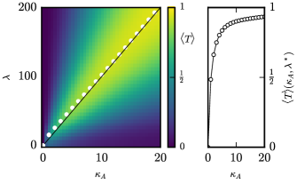
Figure 1: Left panel: Parameter dependence of the average transmission $\left\langle{T}\right\rangle(\kappa_{\mathrm{A}},\lambda)$. The white dots are the optimal values of $\lambda^{*}_{\mathrm{num}}$ obtained by a numerical search for fixed $\kappa_{\mathrm{A}}$. The straight black line is given by Eq. (9) for comparison. Right panel: Average transmission $T(\kappa_{\mathrm{A}},\lambda^{*}_{\mathrm{num}})$ for the numerically obtained optimal parameters. The calculation at each point $\kappa_{\mathrm{A}},\lambda$ is based on $80$ realizations of $100\times 100$ GOE Hamiltonians.

A corresponding plot is shown in Fig. 1. From the figure, one can see that the numerically obtained optimal value $\lambda^{*}_{\mathrm{num}}(\kappa_{\mathrm{A}})$ does tend towards the straight line given by the case without environment in Eq. (9). The same result is obtained when not optimizing numerically for maximal $\left\langle{T}\right\rangle$ but for minimal $\mathrm{Var}\left({T}\right)$ (not shown). At small values of $\kappa_{\mathrm{A}}$ the dependency deviates from the linear form. However, the interesting parameter regime is at large values as this region corresponds to large $\left\langle{T}\right\rangle$, as can be seen from the right panel in Fig. 1. In order to check whether the region

$$\kappa_{\mathrm{A}}\gg 1\qquad\mathrm{and}\qquad\lambda\approx\lambda^{*}\gg 1$$ (14)

is the interesting parameter range, we present three distributions of transmissions along the line in Fig. 2.

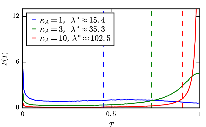
Figure 2: Transmission distribution for three pairs of $\kappa_{\mathrm{A}},\lambda$ values from the numerically obtained optimal curve for maximal average transmission $\left\langle{T}\right\rangle$. The curves belong to increasing value of $\kappa_{\mathrm{A}}$ for blue, green, and red. The dashed lines indicate $\left\langle{T}\right\rangle$ for every curve. The plot emphasizes, that also the variance of the distribution gets smaller for larger values of the parameters. For these curves $8\cdot 10^{5}$ realizations have been used.

In order to get a smooth dependency of $P(T)$, we used $8\cdot 10^{5}$ realizations for each of the curves. The plot clearly shows that the distribution $P(T)$ gets closer to the expression (8) for large values of $\kappa_{\mathrm{A}}$ and $\lambda$.

IV Perturbation Theory

As the most promising parameter region for high transmission can be found for large parameter values (14), we can approach the complex background perturbatively. We can do so by introducing a small parameter $\varepsilon$ in

$$\lambda=\frac{\lambda^{\prime}}{\varepsilon}\hskip 12.91663pt\kappa_{\mathrm{A}}=\frac{\kappa_{\mathrm{A}}^{\prime}}{\varepsilon}\hskip 12.91663ptH_{\mathrm{eff}}^{\prime}=\varepsilon H_{\mathrm{eff}}$$ (15)

which scales the parameters up to large values. With this parametrization, the GOE contribution of the Hamiltonian becomes a small perturbation. With

$$H_{\mathrm{eff}}^{\prime}=\begin{pmatrix}-\mathrm{i}\frac{\kappa_{\mathrm{A}}^{\prime}}{\pi}N&\lambda^{\prime}\frac{\sqrt{N}}{\pi}&0&\\ \lambda^{\prime}\frac{\sqrt{N}}{\pi}&-\mathrm{i}\frac{\kappa_{\mathrm{A}}^{\prime}}{\pi}N&0&\dots\\[4.30554pt] 0&0&0&\\ &\vdots&&\ddots\\ \end{pmatrix}+\varepsilon H_{\mathrm{GOE}}$$ (16)

we can first diagonalize the non-GOE part. The corresponding eigenvalues and eigenvectors are

$$\left(H_{\mathrm{direct}}+\frac{\mathrm{i}}{2}WW^{T}\right){\left|{r^{(0)}_{n}}\right\rangle}=E^{(0)}_{n}{\left|{r^{(0)}_{n}}\right\rangle}.$$ (17)

Although this Hamiltonian is non-hermitian, its symmetric form has right eigenvectors which are equal to the left eigenvectors, ${\left|{l^{(0)}}\right\rangle}={\left|{r^{(0)}}\right\rangle}$. Under the presence of $\varepsilon H_{\mathrm{GOE}}$ we can write the eigenenergies and eigenvectors in first order perturbation theory for non-hermitian operators as [12]

$$\tilde{E}^{(1)}_{n} =E^{(0)}_{n}+\varepsilon E^{(1)}_{n}, {\left|{\tilde{r}^{(1)}_{n}}\right\rangle} ={\left|{r^{(0)}_{n}}\right\rangle}+\epsilon{\left|{r^{(1)}_{n}}\right\rangle}$$ (18)

and arrive at

$$S_{12}=\mathrm{i}\frac{\kappa_{\mathrm{A}}^{\prime}\Delta}{2\pi}N \left({\left\langle{r^{(0)}_{2}}\right|}-{\left\langle{r^{(0)}_{1}}\right|}\right)$$

$$\sum\limits_{n=1}^{2}{\left|{\tilde{r}^{(1)}_{n}}\right\rangle}\frac{1}{\varepsilon E-\tilde{E}^{(1)}_{n}}{\left\langle{\tilde{r}^{(1)}_{n}}\right|}$$ (19)

$$\left({\left|{r^{(0)}_{1}}\right\rangle}+{\left|{r^{(0)}_{2}}\right\rangle}\right).$$

Because all eigenvalues $E_{n}^{(0)}$ of the unperturbed Hamiltonian (16) with $n>2$ are degenerate, the corresponding eigenvectors up to first order are just mixed among each other. Therefore, they are orthogonal to the vectors ${\left|{r^{(0)}_{1}}\right\rangle}\pm{\left|{r^{(0)}_{2}}\right\rangle}$ and do not contribute to $S_{12}$. Hence, only the first two elements of the sum remain thereby effectively reducing the $N(N+1)/2$ independent parameters from the $N\times N$ $H_{\mathrm{GOE}}$ to only $h_{11},h_{12}$, and $h_{22}$. After some algebra we can write

$$S_{12}=-2\mathrm{i}\left(1-z^{2}\right)\frac{y}{(x+\mathrm{i})^{2}-y^{2}}$$ (20)

and therefore

$${\left|{S_{12}}\right|^{2}} =\left(1-z^{2}\right)^{2}\frac{4y^{2}}{\left(x^{2}-y^{2}-1\right)^{2}+4x^{2}}$$ (21)

$$=:\left(1-z^{2}\right)^{2}c(x,y)$$ (22)

where we used the abbreviations

$$x =-\frac{h_{a}}{\kappa_{\mathrm{A}}\sqrt{N}} y =\frac{\lambda}{\kappa_{\mathrm{A}}\sqrt{N}}+\frac{h_{c}}{\kappa_{\mathrm{A}}\sqrt{N}} z =\frac{h_{b}}{2\lambda}.$$ (23)

In these expressions the variables $h_{a,b}:=\pi(h_{11}\pm h_{22})/2\sqrt{N}$ and $h_{c}:=\pi h_{12}/\sqrt{N}$ are normal-distributed $\mathcal{N}(0,1)$ random variables. It follows that the variances read

$$\mathrm{Var}\left({x}\right)=\mathrm{Var}\left({y}\right) =\frac{1}{\kappa_{\mathrm{A}}^{2}N} \mathrm{Var}\left({z}\right) =\frac{1}{4\lambda^{2}}.$$ (24)

With this conventions our main result follows as

$$P(T)= \left\langle{\delta\left(T-{\left|{S_{12}}\right|^{2}}\right)}\right\rangle$$ (25)

$$= \int\!\!\!\!\int\!\mathrm{d}{h_{a}}\frac{\mathrm{e}^{-h_{a}^{2}/2}}{\sqrt{2\pi}}\mathrm{d}{h_{c}}\frac{\mathrm{e}^{-h_{c}^{2}/2}}{\sqrt{2\pi}}\!\frac{\lambda/c}{\sqrt{2\pi}}\frac{1}{\sqrt{{T}/{c}}}$$ (26)

$$\left(\!\frac{\mathrm{e}^{-2\lambda^{2}\left(1+\sqrt{{T}/{c}}\right)}}{\sqrt{1+\sqrt{{T}/{c}}}}\!+\!\Theta\left(c-T\right)\frac{\mathrm{e}^{-2\lambda^{2}\left(1-\sqrt{{T}/{c}}\right)}}{\sqrt{1-\sqrt{{T}/{c}}}}\!\right).$$

The above result can be further simplified when considering the fact that the variances in Eq. (24) go to zero in the interesting limit (14). This allows to evaluate the Gaussians only at their peak. This leads us to

$$c\left(0,\frac{\lambda}{\kappa_{\mathrm{A}}\sqrt{N}}\right)={T_{\mathrm{A}}}\left(\frac{\lambda^{2}}{N\kappa_{\mathrm{A}}^{2}}\right)$$ (27)

and therefore to

$$P(T)\,\approx\, \frac{\lambda/{T_{\mathrm{A}}}}{\sqrt{2\pi}}\frac{1}{\sqrt{{T}/{{T_{\mathrm{A}}}}}}\left(\rule[0.0pt]{0.0pt}{21.52771pt}\right.\frac{\mathrm{e}^{-2\lambda^{2}\left(1+\sqrt{{T}/{{T_{\mathrm{A}}}}}\right)}}{\sqrt{1+\sqrt{{T}/{{T_{\mathrm{A}}}}}}}$$

$$+\Theta\left({T_{\mathrm{A}}}-T\right)\frac{\mathrm{e}^{-2\lambda^{2}\left(1-\sqrt{{T}/{{T_{\mathrm{A}}}}}\right)}}{\sqrt{1-\sqrt{{T}/{{T_{\mathrm{A}}}}}}}\left.\rule[0.0pt]{0.0pt}{21.52771pt}\right).$$ (28)

Note that this treatment is only approximately correct. A proper use of the method of steepest-descent yields a more complicated point for the saddle as it is shifted by the exponential contributions inside the brackets. However, the actual shift turns out to be negligible.

V Numerical Results

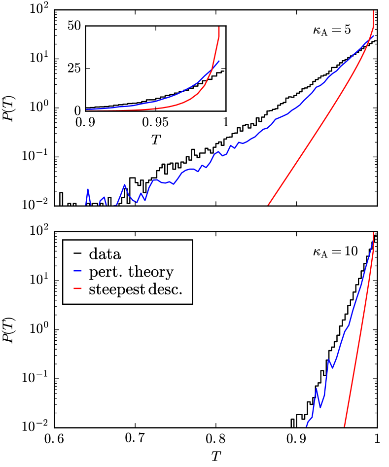
Figure 3: Perturbative prediction of $P(T)$ for $\kappa_{\mathrm{A}}=5$ (upper panel) and $\kappa_{\mathrm{A}}=10$ (lower panel). Shown in black are RMT calculations from $2\times 2$ Hamiltonians for the optimal $\lambda$ from Eq. (9). The calculation was carried out for $8\cdot 10^{3}$ realizations. Shown in blue is the perturbative result (26) while red is the steepest-descent approximation (IV). The upper panel contains an inset in linear scale for comparison.

In order to check the range of validity of the resulting formulas (26) and (IV), we can compare them to RMT calculations as done previously in Fig. 2. The comparison is shown in Fig. 3 for two values of the parameter $\kappa_{\mathrm{A}}=5,10$. While the perturbative results reasonably match the RMT data, the steepest-descent solution proves to be too crude to fully estimate the width of $P(T)$. Note that due to the optimal choice of $\lambda$, Eq. (9), the distribution peaks at $T=1$. In comparison, the solution without any complex background, Eq. (8), is a $\delta$ peak exactly at this value, $P(T)=\delta(T-1)$.

VI Conclusions

This paper presents a physically motivated effective Hamiltonian approach to a common problem of microwave communications. The propagation of electromagnetic fields over PCB boards in the vicinity of obstacles does not allow to use a separation of time scales. This excludes common approaches to account for direct communication paths and makes new models, as the one presented, necessary. By including the direct communication directly into the Hamiltonian, the model allows to determine relevant parameter ranges and a perturbative description of the distribution of transmissions $P(T)$. The resulting approximately exponential decay provides an expression which can be easily compared with experimental data for example from chaotic reverberation chambers (CRCs). In subsequent works we will extract the corresponding parameters from measured transmission and reflection spectra. The above formulas give then rise to distinguish between the stability of several antenna setups (patch, monopole, horn) and give design guidelines for stable communications on small scales.

References

- [1] B. E. Henty and D. D. Stancil, “Multipath-enabled super-resolution for rf and microwave communication using phase-conjugate arrays,” Phys. Rev. Lett., vol. 93, p. 243904, 2004. [Online]. Available: https://dx.doi.org/10.1103/PhysRevLett.93.243904
- [2] P. del Hougne, F. Lemoult, M. Fink, and G. Lerosey, “Spatiotemporal wave front shaping in a microwave cavity,” Phys. Rev. Lett., vol. 117, p. 134302, 2016.
- [3] R. Couillet and M. Debbah, Random Matrix Methods for Wireless Communications. Cambridge: Cambridge University Press, 2011.
- [4] H.-J. Stöckmann, Quantum Chaos - An Introduction. Cambridge: University Press, 2007.
- [5] C. Mahaux and H. A. Weidenmüller, Shell-Model Approach to Nuclear Reactions. Amsterdam: North-Holland, 1969.
- [6] V. V. Sokolov and V. G. Zelevinsky, “Dynamics and statistics of unstable quantum states,” Nucl. Phys. A, vol. 504, p. 562, 1989.
- [7] U. Kuhl, O. Legrand, and F. Mortessagne, “Microwave experiments using open chaotic cavities in the realm of the effective Hamiltonian formalism,” Fortschritte der Physik, vol. 61, p. 404, 2013.
- [8] J. J. M. Verbaarschot, H. A. Weidenmüller, and M. R. Zirnbauer, “Grassmann integration in stochastic quantum physics: The case of compound-nucleus scattering,” Phys. Rep., vol. 129, p. 367, 1985.
- [9] H. Nishioka and H. A. Weidenmüller, “Compound-nucleus scattering in the presence of direct reactions,” Phys. Lett. B, vol. 157, p. 101, 1985.
- [10] S. Hemmady, X. Zheng, J. Hart, T. M. Antonsen Jr., E. Ott, and S. M. Anlage, “Universal properties of two-port scattering, impedance, and admittance matrices of wave-chaotic systems,” Phys. Rev. E, vol. 74, p. 036213, 2006.
- [11] N. Lehmann, D. Saher, V. V. Sokolov, and H.-J. Sommers, “Chaotic scattering: the supersymmetry method for large number of channels,” Nucl. Phys. A, vol. 582, p. 223, 1995.
- [12] Y. V. Fyodorov and D. V. Savin, “Statistics of resonance width shifts as a signature of eigenfunction nonorthogonality,” Phys. Rev. Lett., vol. 108, p. 184101, 2012. [Online]. Available: http://link.aps.org/doi/10.1103/PhysRevLett.108.184101
- [13] “Nemf21: Noisy Electromagnetic Fields – A Technological Platform for Chip-to-Chip Communication in the Century.” see http://www.nemf21.org for detail on the reseach programme and activities.