Probing crustal structures from neutron star compactness

Abstract

With various sets of the parameters that characterize the equation of state (EOS) of nuclear matter, we systematically examine the thickness of a neutron star crust and of the pasta phases contained therein. Then, with respect to the thickness of the phase of spherical nuclei, the thickness of the cylindrical phase, and the crust thickness, we successfully derive fitting formulas that express the ratio of each thickness to the star’s radius as a function of the star’s compactness, the incompressibility of symmetric nuclear matter, and the density dependence of the symmetry energy. In particular, we find that the thickness of the phase of spherical nuclei has such a strong dependence on the stellar compactness as the crust thickness, but both of them show a much weaker dependence on the EOS parameters. Thus, via determination of the compactness, the thickness of the phase of spherical nuclei as well as the crust thickness can be constrained reasonably, even if the EOS parameters remain to be well-determined.

1 Introduction

Neutron stars help to probe the physics in extreme conditions mainly because the star is so compact that the density inside the star can be significantly beyond normal nuclear density (Haensel, Potekhin & Yakovlev, 2007). Moreover, the surface magnetic field can be as high as $\sim 10^{15}$ G (Kouveliotou et al., 1998; Hurley et al., 1999), while the rotation period can be as short as $\sim$msec (Pulsar Group, 2016). Thus, observations of neutron star phenomena associated with such compactness, high magnetic fields, and/or rapid rotation could leave an imprint of the properties of matter under such extreme conditions. However, the neutron star structure has yet to be fixed, because the equation of state (EOS) of matter in the star is still uncertain especially for a high density region. Even so, a conceptual picture of the neutron star structure is theoretically established.

Just below the star’s surface lies an ocean composed of iron, under which matter forms a lattice structure due to the Coulomb interaction. This region is called a crust, where the matter behaves as a solid (or as a liquid crystal). The region below the crust corresponds to a core, where the matter becomes uniform and behaves as a fluid. The density at the base of the crust is expected to lie between $\sim(1/3$–$1)$ times normal nuclear density, depending on the EOS of nuclear matter (Oyamatsu & Iida, 2007). This EOS is often characterized by several parameters that determine the Taylor expansion with respect to the nucleon density and neutron excess around the saturation point of symmetric nuclear matter (Lattimer, 1981), which in turn can be constrained from terrestrial nuclear experiments (Oyamatsu & Iida, 2003; Tsang et al., 2012). One of the key parameters that control the properties of matter in the crust thickness is known to be the slope parameter $L$ of the symmetry energy (Oyamatsu & Iida, 2007), which has yet to be fixed (Li, 2017). This means that one may be able to extract the value of $L$ from astronomical observations. In fact, after the discoveries of quasi-periodic oscillations in the soft-gamma repeaters (Watts & Strohmayer, 2006), attempts to constrain $L$ have been done by identifying the observed frequencies as the crustal torsional oscillations (Steiner & Watts, 2009; Gearheart et al., 2011; Sotani et al., 2012, 2013a, 2013b; Sotani, 2014, 2016; Sotani, Iida & Oyamatsu, 2016).

Additionally, the possible presence of non-spherical (pasta) nuclei in the deepest region of the crust of cold neutron stars has been theoretically considered since Lorenz, Ravenhall & Pethick (1993); Oyamatsu (1993) (see also Pethick & Ravenhall (1995) for early studies on pasta nuclei in collapsing stellar cores and neutron star crusts). As the density increases, the shape of nuclei changes from spherical (SP) to cylindrical (C), slab-like (S), cylindrical-hole (CH), and spherical-hole (SH) shapes before the matter becomes uniform. Whether the pasta structures exist or not depends strongly on $L$ (Oyamatsu & Iida, 2007). It is also suggested that observations of the crustal torsional oscillations enable us to extract the information about the pasta structures (Sotani, 2011; Passamonti & Pons, 2016; Sotani, Iida & Oyamatsu, 2017). We also remark that elaborate dynamical model calculations of the pasta structures have been done at conditions marginally relevant for cold neutron stars (Watanabe et al., 2003; Sébille, de la Mota & Figerou, 2011; Dorso, Giménez Molinelli & López, 2012; Schuetrumpf et al., 2014; Caplan et al., 2015). The possibility that more complicated structures than the above-mentioned shapes may occur even at zero temperature has been suggested, but in this work we assume that the density region where such structures occur is negligible.

In spite of progress in theoretical researches, observational evidences for the presence of the pasta phases, let alone observational constraints on the thickness of such phases, are basically lacking. This is partly because the crust thickness is at most $\sim 10\%$ of the radius of a neutron star with canonical mass and partly because even the star’s mass and radius are hard to determine from observations. On the other hand, the properties of the crust including the pasta structures could be important to the thermal evolution (Newton et al., 2013; Horowitz et al., 2015) and rotational evolution (Pons, Viganò & Rea, 2013) of neutron stars. Via observations associated with such evolutions, one could deduce the crustal properties.

In this paper, we focus on how the thickness of the neutron star crust and the pasta phases depends on the compactness and EOS parameters. For this purpose, we first obtain the equilibrium crust models by numerically integrating the Tolman-Oppenheimer-Volkoff (TOV) equations together with an appropriate crust EOS, and then present a qualitative description of such thickness by simply combining the TOV equations with the Gibbs-Duhem relation. After that, we construct fitting formulas for such thickness from the equilibrium crust models obtained above. We find that the thickness of the phase of spherical nuclei is strong function of the compactness, but relatively weak function of the EOS parameters, and confirm the known compactness dependence of the crust thickness. Then, such thickness could be extracted from determination of the compactness within $\sim 10\%$ accuracy, independent of the EOS parameters. We use units in which $c=G=1$, where $c$ and $G$ denote the speed of light and the gravitational constant, respectively. Note that the compactness becomes a dimensionless parameter with the present units.

2 Models for Neutron Star Crusts

We start with construction of equilibrium neutron star crusts. For this purpose, it is convenient to write down the bulk energy per baryon of uniform nuclear matter at zero temperature in the vicinity of the saturation density, $n_{0}$, of symmetric nuclear matter as a function of baryon number density, $n_{\rm b}$, and neutron excess, $\alpha$, with four coefficients ($w_{0}$, $K_{0}$, $S_{0}$, and $L$) (Lattimer, 1981):

$$w=w_{0}+\frac{K_{0}}{18n_{0}^{2}}(n_{\rm b}-n_{0})^{2}+\left[S_{0}+\frac{L}{3n_{0}}(n_{\rm b}-n_{0})\right]\alpha^{2}.$$ (1)

These coefficients and $n_{0}$ play the role of the saturation parameters, and each EOS has a corresponding set of the saturation parameters. The saturation parameters have been gradually well constrained from terrestrial nuclear experiments, while among the five the incompressibility of symmetric nuclear matter, $K_{0}$, and the slope parameter, $L$, which are higher order coefficients with respect to density change from $n_{0}$, are relatively difficult to determine. Thus, in describing the dependence of the crustal structure on the EOS of nuclear matter, we regard $K_{0}$ and $L$ as free parameters and fix the other saturation parameters ($n_{0}$, $w_{0}$, and $S_{0}$) in such a way as to reproduce empirical data for masses and charge radii of stable nuclei. In practice, we do so by using the phenomenological EOSs of nuclear matter constructed within the framework of the Thomas-Fermi theory by Oyamatsu & Iida (2003). The EOSs of beta-equilibrated, neutral matter in the crust were derived within the same framework from the above EOS of nuclear matter by Oyamatsu & Iida (2007) (see also Iida & Oyamatsu (2014)). Hereafter, we refer to such EOSs as OI-EOSs. We remark that instead of $K_{0}$ and $L$, the OI-EOSs are originally characterized by $K_{0}$ and $y$, where $y$ is defined as $y=-K_{0}S_{0}/(3n_{0}L)$, and that one can easily determine the value of $L$ for given $y$. In Table 1, we show the sets of the saturation parameters that are adopted in this work. Here, even extreme cases are effectively covered (Oyamatsu & Iida, 2003), as compared to typical values obtained from terrestrial experiments, e.g., $K_{0}=230\pm 40$ MeV (Khan & Margueron, 2013) or $250<K_{0}<315$ MeV (Stone, Stone & Moszkowski, 2014), and $30\,\,\raisebox{-3.44444pt}{$\stackrel{{\scriptstyle\textstyle<}}{{\sim}}$ }L\,\,\raisebox{-3.44444pt}{$\stackrel{{\scriptstyle\textstyle<}}{{\sim}}$ }80$ MeV (Newton et al., 2014).

In order to construct neutron star models, one generally needs to prepare the EOS of matter in the star ranging from the star’s surface down to center. However, the EOS of matter in the core, particularly in the density region higher than a few times normal nuclear density, is still uncertain. To avoid such uncertainties, we construct the crust of a non-rotating neutron star with mass $M$ and radius $R$ by integrating the TOV equations from the star’s surface inward down to the base of the crust, as in Iida & Sato (1997); Sotani et al. (2012); Sotani, Iida & Oyamatsu (2017). In this work, we focus on the stellar models with $1.4\leq M/M_{\odot}\leq 1.8$ and $10\leq R\leq 14$ km. Now, the crustal structure thus constructed is controlled by the four parameters, namely, the EOS parameters $K_{0}$ and $L$ and the neutron star parameters $M$ and $R$. We remark in passing that the layer of the ocean is so thin that we can safely neglect the the ocean thickness in calculating the crust thickness.

As mentioned above, the shapes of nuclei can change from spherical to cylindrical, slab-like, cylindrical-hole, and spherical-hole before the matter becomes uniform. The densities at the respective phase transitions depend on the saturation parameters (Oyamatsu & Iida, 2007). In fact, for the EOS parameter sets adopted in this paper, the transition densities are listed in Table 1.

Table 1: The SP-C, C-S, S-CH, CH-SH, and SH-U transition densities obtained for various sets of the EOS parameters, which are characterized by $K_{0}$ and $L$. The asterisk at the value of $K_{0}$ denotes the EOS model by which some pasta phases are not predicted to appear. That is, the values with *1, *2, and *3 denote the transition densities from cylindrical nuclei to uniform matter, from cylindrical-hole nuclei to uniform matter, and from spherical nuclei to uniform matter, respectively.

$K_{0}$ (MeV)	$-y$ (MeV fm3)	$L$ (MeV)	SP-C (fm-3)	C-S (fm-3)	S-CH (fm-3)	CH-SH (fm-3)	SH-U (fm-3)
180	1800	5.7	0.06000	0.08665	0.12039	0.12925	0.13489
180	600	17.5	0.05849	0.07986	0.09811	0.10206	0.10321
180	350	31.0	0.05887	0.07629	0.08739	0.09000	0.09068
180	220	52.2	0.06000	0.07186	0.07733	0.07885	0.07899
230	1800	7.6	0.05816	0.08355	0.11440	0.12364	0.12736
230	600	23.7	0.05957	0.07997	0.09515	0.09817	0.09866
230	350	42.6	0.06238	0.07671	0.08411	0.08604	0.08637
230	220	73.4	0.06421	0.07099	0.07284	0.07344	0.07345
280	1800	9.6	0.05747	0.08224	0.11106	0.11793	0.12286
280	600	30.1	0.06218	0.08108	0.09371	0.09577	0.09623
280	350	54.9	0.06638	0.07743	0.08187	0.08314	0.08331
∗280	220	97.5	0.06678	—	—	—	0.06887∗1
360	1800	12.8	0.05777	0.08217	0.10892	0.11477	0.11812
360	600	40.9	0.06743	0.08318	0.09197	0.09379	0.09414
∗360	350	76.4	0.07239	0.07797	0.07890	—	0.07918∗2
∗360	220	146.1	—	—	—	—	0.06680∗3

Table 2: Same as Table 1 but for the neutron chemical potential, including the rest mass, at the phase transitions.

$K_{0}$ (MeV)	$-y$ (MeV fm3)	$L$ (MeV)	SP-C (MeV)	C-S (MeV)	S-CH (MeV)	CH-SH (MeV)	SH-U (MeV)
180	1800	5.7	951.041	952.272	952.918	953.151	953.291
180	600	17.5	950.667	952.004	952.971	953.175	953.232
180	350	31.0	950.318	951.712	952.434	952.680	952.747
180	220	52.2	949.839	951.114	951.611	951.812	951.831
230	1800	7.6	950.915	952.195	953.119	953.208	953.319
230	600	23.7	950.583	952.069	952.915	953.176	953.219
230	350	42.6	950.307	951.779	952.441	952.689	952.732
230	220	73.4	949.931	950.949	951.196	951.304	951.305
280	1800	9.6	950.837	952.169	952.904	953.168	953.400
280	600	30.1	950.625	952.224	953.286	953.459	953.496
280	350	54.9	950.552	952.050	952.571	952.780	952.807
∗280	220	97.5	950.344	—	—	—	950.743∗1
360	1800	12.8	950.812	952.244	953.307	953.397	953.611
360	600	40.9	950.968	952.756	953.806	954.014	954.051
∗360	350	76.4	951.535	951.929	951.995	—	952.014∗2
∗360	220	146.1	—	—	—	—	951.277∗3

3 Formulas for the thickness of the pasta phases and the whole crust

In this section, we derive fitting formulas for the thickness of the whole and parts of the neutron star crust constructed in the previous section. Before going into details, we give a qualitative description of such thickness by combining the TOV equations with the Gibbs-Duhem relation as

$$\Delta R_{AB}\simeq\frac{(R-C\Delta R_{AB})^{2}[1-2M/(R-C\Delta R_{AB})]}{m_{n}M}(\mu_{B}-\mu_{A}),$$ (2)

where $\Delta R_{AB}$ is the crust thickness between two radii $B$ (lower) and $A$ (upper), $m_{n}$ is the neutron rest mass, $\mu_{A}$ and $\mu_{B}$ are the neutron chemical potentials including $m_{n}$ at the radii $A$ and $B$, and $C$ is a constant that comes from the mean-value theorem and satisfies $0\leq C\leq 1$. In Eq. (2), the pressure is ignored as compared with the mass density, which is in turn approximated as $m_{n}$ times baryon density. We also assume that the mass of the crust is negligibly small compared with $M$. Instead of solving Eq. (2) with respect to $\Delta R_{AB}$, we can obtain an approximate solution by setting $C=0$ as (Pethick & Ravenhall, 1995)

$$\Delta R_{AB}\simeq\frac{R^{2}(1-2M/R)}{m_{n}M}(\mu_{B}-\mu_{A}).$$ (3)

We find from this expression that the ratio of the thickness $\Delta R_{AB}$ to $R$ is controlled by the compactness $M/R$ via the factor $R/M(1-2M/R)$ and also by the neutron chemical potential difference $\mu_{B}-\mu_{A}$. Eventually, by comparing with numerical results that will be given below, expression (3) turns out to be successful in reproducing the $L$, $K_{0}$, and $M/R$ dependence of the thickness of the crust and pasta phases qualitatively, while deviations from the numerical results are at most a factor of two. Incidentally, all the values of $\mu_{A}$ and $\mu_{B}$ to be given in Eq. (3) are listed in Table 2, except in the case of the thickness of the crust and the spherical phase in which $\mu_{A}$ is set to $m_{n}$. We remark that Zdunik & Haensel (2011); Zdunik, Fortin & Haensel (2017) have also derived the approximate relation between the crust thickness and the stellar compactness by ignoring the pressure correction terms in the TOV equations as we do in Eq. (2).

To examine how the chemical potential difference $\mu_{B}-\mu_{A}$ depends on the EOS parameters, it is convenient to obtain the expansion form of the neutron chemical potential from Eq. (1) as

$$\mu_{n}=m_{n}+w_{0}+S_{0}\alpha(2-\alpha)+\frac{n_{b}-n_{0}}{18n_{0}}\left(12L\alpha+K_{0}\frac{3n_{b}-n_{0}}{n_{0}}\right)+\frac{L}{3}\alpha^{2},$$ (4)

This expression clearly shows the $L$ and $K_{0}$ contributions to $\mu_{n}$. Although Eq. (4) is strictly valid near $n_{b}=n_{0}$ and $\alpha=0$, it is instructive to extrapolate it to the regime of $n_{b}$ and $\alpha$ relevant to the deepest region of the crust, i.e., subnuclear densities and extremely large neutron excess. Note that all the transition densities listed in Table 1 (see also Fig. 1 of Sotani, Iida & Oyamatsu (2017)) lies between $n_{0}/3$ and $n_{0}$ and that a gas of dripped neutrons occupy more than $\sim$70% of the nucleons. Thus, we can simply set $\alpha=1$, which gives rise to $w_{0}+S_{0}+L/3$ as a constant part of $\mu_{n}-m_{n}$. This part is typically of order 10–40 MeV. The remaining density-dependent part, which is negative and roughly of order 10 MeV, controls the EOS dependence of the thickness of each pasta-like nonspherical phase because the constant part is essentially cancelled in the difference $\mu_{B}-\mu_{A}$. This EOS dependence is complicated by the fact that the transition densities themselves depend on $L$ and $K_{0}$ as in Table 1. Anyway, according to Eq. (4), the $L$ dependence of $\mu_{B}-\mu_{A}$ is dominant over the $K_{0}$ dependence, which will play a role in parametrizing the thickness of the pasta phases as a function of $M/R$, $L$, and $K_{0}$.

The thickness of the spherical phase needs to be examined separately. In this case, the constant part $w_{0}+S_{0}+L/3$ contributes to the $L$ dependence of $\mu_{B}-\mu_{A}$ (here, $\mu_{A}=m_{n}$) in such a way that the $L$ dependence that comes from the density-dependent part as shown above is weakened. Since the SP-C transition density is about $n_{0}/3$ and almost independent of $L$ and $K_{0}$, furthermore, the thickness of the spherical phase is expected to depend only weakly on $L$ and $K_{0}$. This expectation looks consistent with the behavior of $\mu_{n}$ that can be seen from Table 2. We remark that the thickness of the whole crust, which is dominated by the thickness of the spherical phase, has a similarly weak EOS dependence.

As a typical thickness of the whole crust, we will thus use

$$\frac{\Delta R}{R}\simeq 2.1\times 10^{-2}\frac{R}{M}\left(1-\frac{2M}{R}\right),$$ (5)

which is based on Eq. (2) and is independent of $L$ and $K_{0}$. Here, the factor $2.1\times 10^{-2}$ is slightly different from the factor $2.57\times 10^{-2}$ that were obtained by calculating the factor $\mu_{B}/m_{n}-1$ in Eq. (3) from the EOS of FPS (Ravenhall & Pethick, 1994). Note that the factor $2.1\times 10^{-2}$ effectively allows for nonzero $C$ in contrast to the factor $2.57\times 10^{-2}$. We remark that Zdunik & Haensel (2011); Zdunik, Fortin & Haensel (2017) have also indicated the strong compactness dependence of the relative crust thickness, while studying the effects of accretion and rotation. In the present work, we try to derive a fitting formula for the thickness of the whole crust by including the detailed $L$ and $K_{0}$ dependence. Before doing so, in the following subsections, we consider the thickness of the SP phase and of each pasta phase.

3.1 Phase of spherical (SP) nuclei

By using the neutron star crusts constructed in Sec. 2 for nine stellar models with the combinations of three different masses ($M/M_{\odot}=1.4$, 1.6, and 1.8) and three different radii ($R=10$, 12, and 14 km), let us now examine the compactness and EOS dependence of the thickness, $\Delta R_{\rm sp}$, of the phase composed of the spherical nuclei. In Fig. 1, we show the ratio of $\Delta R_{\rm sp}$ to $R$ as a function of $R/M$, which is the reciprocal of the stellar compactness, for various sets of $L$ and $K_{0}$. From this figure, we find that $\Delta R_{\rm sp}/R$ can be well expressed as a function of $R/M$ for each set of the EOS parameters:

$$\frac{\Delta R_{\rm sp}}{R}=-\alpha_{1}^{\rm sp}\left(\frac{R}{M}\right)^{2}+\alpha_{2}^{\rm sp}\left(\frac{R}{M}\right)-\alpha_{3}^{\rm sp},$$ (6)

where $\alpha_{1}^{\rm sp}$, $\alpha_{2}^{\rm sp}$, and $\alpha_{3}^{\rm sp}$ are positive dimensionless adjustable coefficients that depend on ($L$, $K_{0}$). Note that this form arises from Eq. (2) in which the parameter $C$ is taken to be order unity. We can then expect $\alpha_{1}^{\rm sp}$ to be small compared with $\alpha_{2}^{\rm sp}$ and $\alpha_{3}^{\rm sp}$. In Fig. 1, we can confirm that expression (6) does accurately reproduce $\Delta R_{\rm sp}/R$ for each set of the EOS parameters. In addition, one can observe that $\Delta R_{\rm sp}/R$ strongly depends on the stellar compactness, while the dependence on the EOS parameters is relatively weak, as expected from the above-mentioned arguments. That is, one can deduce the value of $\Delta R_{\rm sp}/R$ once the stellar compactness is observationally determined.

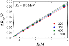
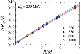
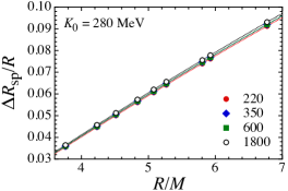
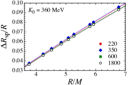
Figure 1: The ratio of the thickness of the phase composed of spherical nuclei to the star’s radius, which was obtained from various OI-EOSs, as a function of the inverse of the compactness $M/R$. The upper-left, upper-right, lower-left, and lower-right panels correspond to the cases of $K_{0}=180$, 230, 280, and 360 MeV, while the solid-circles, solid-diamonds, solid-squares, and open-circles in each panel are the results obtained for $-y=220$, $350$, $600$, and $1800$ MeV fm³. The dotted lines denote the fitting formula given by Eq. (6).

We then move on to express the coefficients in Eq. (6) as a function of the EOS parameters $(L,K_{0})$. In Fig. 2 we plot the values of $\alpha_{i}^{\rm sp}$ with $i=1$, 2, and 3, which were obtained by fitting for several sets of $K_{0}$ and $L$. From this figure, we find that $\alpha_{i}^{\rm sp}$ with $i=1$, 2, and 3 can be expressed as a function of $L$ for $K_{0}=180$, 230, and 280 MeV by

$$\alpha_{1}^{\rm sp} = \beta_{11}^{\rm sp}\left(\frac{L}{60\ {\rm MeV}}\right)^{-1}+\beta_{12}^{\rm sp}-\beta_{13}^{\rm sp}\left(\frac{L}{60\ {\rm MeV}}\right),$$ (7)

$$\alpha_{2}^{\rm sp} = \beta_{21}^{\rm sp}\left(\frac{L}{60\ {\rm MeV}}\right)^{-1}+\beta_{22}^{\rm sp}-\beta_{23}^{\rm sp}\left(\frac{L}{60\ {\rm MeV}}\right),$$ (8)

$$\alpha_{3}^{\rm sp} = \beta_{31}^{\rm sp}\left(\frac{L}{60\ {\rm MeV}}\right)^{-1}+\beta_{32}^{\rm sp}-\beta_{33}^{\rm sp}\left(\frac{L}{60\ {\rm MeV}}\right),$$ (9)

where $\beta_{ij}^{\rm sp}$ with $i=1$, 2, 3 and $j=1$, 2, 3 are positive dimensionless fitting parameters that depend on $K_{0}$. Figure 2 shows that expressions (7)–(9) accurately reproduce the $L$ dependence of the coefficients in Eq. (6) for $K_{0}=180$, 230, 280 MeV. We remark that this is not the case with $K_{0}=360$ MeV, but this value of $K_{0}$ is obviously beyond the constraint from the terrestrial experiments (e.g., Khan & Margueron (2013); Stone, Stone & Moszkowski (2014)).

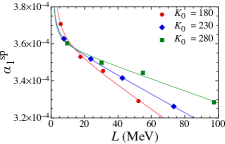
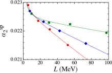
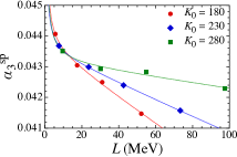
Figure 2: The coefficients in Eq. (6), shown as a function of $L$. The circles, diamonds, and squares are the results of $K_{0}=180$, 230, and 280 MeV. The dotted lines in each panel denote the fitting formula given by Eqs. (7)–(9).

Finally, we construct the fitting formula for the coefficients in Eqs. (7)–(9) as a function of $K_{0}$. In Fig. 3, we plot the values of $\beta_{ij}^{\rm sp}$ obtained by fitting for $K_{0}=180,230,280$ MeV as shown in Fig. 2. From Fig. 3, we find that the values of $\beta_{ij}^{\rm sp}$ can then be fitted as a linear function of $K_{0}$:

$$\beta_{11}^{\rm sp} = \left[2.3515-1.5395\left(\frac{K_{0}}{230\ {\rm MeV}}\right)\right]\times 10^{-6},$$ (10)

$$\beta_{12}^{\rm sp} = \left[3.6353-0.02852\left(\frac{K_{0}}{230\ {\rm MeV}}\right)\right]\times 10^{-4},$$ (11)

$$\beta_{13}^{\rm sp} = \left[7.0703-4.2055\left(\frac{K_{0}}{230\ {\rm MeV}}\right)\right]\times 10^{-5},$$ (12)

$$\beta_{21}^{\rm sp} = \left[2.8280+0.5881\left(\frac{K_{0}}{230\ {\rm MeV}}\right)\right]\times 10^{-5},$$ (13)

$$\beta_{22}^{\rm sp} = \left[2.3107-0.05589\left(\frac{K_{0}}{230\ {\rm MeV}}\right)\right]\times 10^{-2},$$ (14)

$$\beta_{23}^{\rm sp} = \left[3.2551-2.4233\left(\frac{K_{0}}{230\ {\rm MeV}}\right)\right]\times 10^{-3},$$ (15)

$$\beta_{31}^{\rm sp} = \left[0.4770+0.1564\left(\frac{K_{0}}{230\ {\rm MeV}}\right)\right]\times 10^{-4},$$ (16)

$$\beta_{32}^{\rm sp} = \left[4.4481-0.1081\left(\frac{K_{0}}{230\ {\rm MeV}}\right)\right]\times 10^{-2},$$ (17)

$$\beta_{33}^{\rm sp} = \left[6.0989-4.5574\left(\frac{K_{0}}{230\ {\rm MeV}}\right)\right]\times 10^{-3}.$$ (18)

Now, we obtain a complete set of the fitting formulas (6)–(18), which well reproduces the calculated values of $\Delta R_{\rm sp}/R$ for various combinations of $R/M$, $L$, and $K_{0}$. Note that applicability of these formulas is limited to the range of $180\,\,\raisebox{-3.44444pt}{$\stackrel{{\scriptstyle\textstyle<}}{{\sim}}$ }K_{0}\,\,\raisebox{-3.44444pt}{$\stackrel{{\scriptstyle\textstyle<}}{{\sim}}$ }280$ MeV.

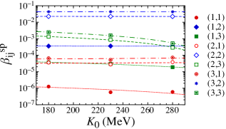
Figure 3: The coefficients in Eqs. (7)–(9) plotted as a function of $K_{0}$, where the labels of $(i,j)$ for $i=1,2,3$ and $j=1,2,3$ denote the subscript in $\beta_{ij}^{\rm sp}$. The dotted, dashed, and dot-dashed lines denote the fitting formula for $i=1$, 2, and 3, respectively.

3.2 Phase of cylindrical (C) nuclei

Next, we turn to the thickness of the phase composed of cylindrical nuclei, $\Delta R_{\rm cy}$. We find again that $\Delta R_{\rm cy}/R$ can be well expressed as a function of $R/M$ for each set of the EOS parameters, as shown in Fig. 4, i.e., we can derive the fitting formula for $\Delta R_{\rm cy}/R$ by

$$\frac{\Delta R_{\rm cy}}{R}=-\alpha_{1}^{\rm cy}\left(\frac{R}{M}\right)^{2}+\alpha_{2}^{\rm cy}\left(\frac{R}{M}\right)-\alpha_{3}^{\rm cy},$$ (19)

where $\alpha_{1}^{\rm cy}$, $\alpha_{2}^{\rm cy}$, and $\alpha_{3}^{\rm cy}$ are positive dimensionless adjustable coefficients that depend on $(L,K_{0})$. We notice that $\Delta R_{\rm cy}$ reduces to zero in the case of $(K_{0},-y)=(360\ {\rm MeV},220\ {\rm MeV\ fm}^{3})$ in which the spherical nuclei melt into uniform matter instead of changing into cylindrical ones. We also find that $\Delta R_{\rm cy}/R$ depends on the EOS parameters as strongly as $R/M$, which is a contrast to the case of $\Delta R_{\rm sp}/R$ but expected from the arguments based on Eq. (4).

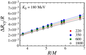
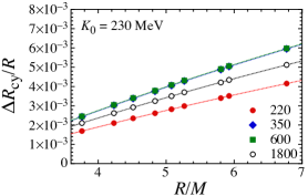
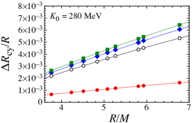
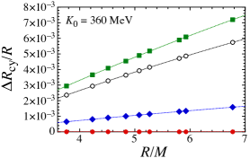
Figure 4: Same as Fig. 1, but for the ratio of the thickness of the phase composed of cylindrical nuclei to the star’s radius. The dotted lines denote the fitting formula given by Eq. (19).

In a similar way to the case of $\Delta R_{\rm sp}/R$, we plot in Fig. 5 the values of $\alpha_{1}^{\rm cy}$, $\alpha_{2}^{\rm cy}$, and $\alpha_{3}^{\rm cy}$, which were obtained by fitting for several sets of $K_{0}$ and $L$, as a function of $L$. These values can then be accurately expressed by the following fitting formulas:

$$\alpha_{1}^{\rm cy} = \beta_{11}^{\rm cy}+\beta_{12}^{\rm cy}\left(\frac{L}{60\ {\rm MeV}}\right)-\beta_{13}^{\rm cy}\left(\frac{L}{60\ {\rm MeV}}\right)^{2},$$ (20)

$$\alpha_{2}^{\rm cy} = \beta_{21}^{\rm cy}+\beta_{22}^{\rm cy}\left(\frac{L}{60\ {\rm MeV}}\right)-\beta_{23}^{\rm cy}\left(\frac{L}{60\ {\rm MeV}}\right)^{2},$$ (21)

$$\alpha_{3}^{\rm cy} = \beta_{31}^{\rm cy}+\beta_{32}^{\rm cy}\left(\frac{L}{60\ {\rm MeV}}\right)-\beta_{33}^{\rm cy}\left(\frac{L}{60\ {\rm MeV}}\right)^{2},$$ (22)

where $\beta_{ij}^{\rm cy}$ with $i=1$, 2, 3 and $j=1$, 2, 3 are positive dimensionless adjustable coefficients that depend on $K_{0}$. Again, such fitting does not work well for $K_{0}=360$ MeV. We note that the functional form of $\alpha_{i}^{\rm cy}$ with respect to $L$ is different from that of $\alpha_{i}^{\rm sp}$.

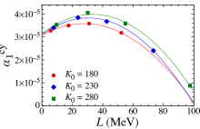
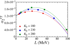
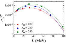
Figure 5: Same as Fig. 2, but for the coefficients in Eq. (19) and the fitting formula given by Eqs. (20)–(22).

In Fig. 6, the values of $\beta_{ij}^{\rm cy}$ with $i=1$, 2, 3 and $j=1$, 2, 3, obtained by fitting for $K_{0}=180,230,280$ MeV, are shown as a function of $K_{0}$. From this figure, we find that $\beta_{ij}^{\rm cy}$ can be accurately expressed as a linear function of $K_{0}$,

$$\beta_{11}^{\rm cy} = \left[2.9604+0.1490\left(\frac{K_{0}}{230\ {\rm MeV}}\right)\right]\times 10^{-5},$$ (23)

$$\beta_{12}^{\rm cy} = \left[0.7194+1.9688\left(\frac{K_{0}}{230\ {\rm MeV}}\right)\right]\times 10^{-5},$$ (24)

$$\beta_{13}^{\rm cy} = \left[1.8003+0.8342\left(\frac{K_{0}}{230\ {\rm MeV}}\right)\right]\times 10^{-5},$$ (25)

$$\beta_{21}^{\rm cy} = \left[1.2506-0.03795\left(\frac{K_{0}}{230\ {\rm MeV}}\right)\right]\times 10^{-3},$$ (26)

$$\beta_{22}^{\rm cy} = \left[-0.02827+1.3325\left(\frac{K_{0}}{230\ {\rm MeV}}\right)\right]\times 10^{-3},$$ (27)

$$\beta_{23}^{\rm cy} = \left[0.4456+0.6976\left(\frac{K_{0}}{230\ {\rm MeV}}\right)\right]\times 10^{-3},$$ (28)

$$\beta_{31}^{\rm cy} = \left[2.3235-0.06992\left(\frac{K_{0}}{230\ {\rm MeV}}\right)\right]\times 10^{-3},$$ (29)

$$\beta_{32}^{\rm cy} = \left[-0.03548+2.4785\left(\frac{K_{0}}{230\ {\rm MeV}}\right)\right]\times 10^{-3},$$ (30)

$$\beta_{33}^{\rm cy} = \left[0.8266+1.3062\left(\frac{K_{0}}{230\ {\rm MeV}}\right)\right]\times 10^{-3}.$$ (31)

Now, we obtain a complete set of the fitting formulas (19)–(31), which well reproduce the calculated values of $\Delta R_{\rm cy}/R$ for various combinations of $R/M$, $L$, and $K_{0}$. Note that applicability of these formulas is here again limited to the range of $180\,\,\raisebox{-3.44444pt}{$\stackrel{{\scriptstyle\textstyle<}}{{\sim}}$ }K_{0}\,\,\raisebox{-3.44444pt}{$\stackrel{{\scriptstyle\textstyle<}}{{\sim}}$ }280$ MeV.

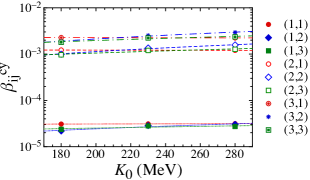
Figure 6: Same as Fig. 3, but for the coefficients in Eqs. (20)–(22) and the corresponding fitting formulas.

3.3 Phases of slab-like (S), cylindrical-hole (CH), and spherical-hole (SH) nuclei

We now focus on the rest of the pasta phases, namely, the S, CH, and SH phases. For various sets of the EOS parameters, the calculated relative thickness of the layer of slab-like nuclei, $\Delta R_{\rm sl}/R$, that of the layer of cylindrical-hole nuclei, $\Delta R_{\rm ch}/R$, and that of the layer of spherical-hole nuclei, $\Delta R_{\rm sh}/R$, are shown in Figs. 7, 8, and 9, respectively, as a function of $R/M$. From these figures, we can confirm that $\Delta R_{\rm sl}/R$, $\Delta R_{\rm ch}/R$, and $\Delta R_{\rm sh}/R$ can be accurately expressed as a function of $R/M$ by

$$\frac{\Delta R_{\rm sl}}{R} = -\alpha_{1}^{\rm sl}\left(\frac{R}{M}\right)^{2}+\alpha_{2}^{\rm sl}\left(\frac{R}{M}\right)-\alpha_{3}^{\rm sl},$$ (32)

$$\frac{\Delta R_{\rm ch}}{R} = -\alpha_{1}^{\rm ch}\left(\frac{R}{M}\right)^{2}+\alpha_{2}^{\rm ch}\left(\frac{R}{M}\right)-\alpha_{3}^{\rm ch},$$ (33)

$$\frac{\Delta R_{\rm sh}}{R} = -\alpha_{1}^{\rm sh}\left(\frac{R}{M}\right)^{2}+\alpha_{2}^{\rm sh}\left(\frac{R}{M}\right)-\alpha_{3}^{\rm sh},$$ (34)

where $\alpha_{i}^{\rm sl}$, $\alpha_{i}^{\rm ch}$, and $\alpha_{i}^{\rm sh}$ with $i=1$, 2, 3 are positive dimensionless adjustable coefficients, tabulated in Tables 3, 4, and 5. One can observe that $\Delta R_{\rm sl}/R$, $\Delta R_{\rm ch}/R$, and $\Delta R_{\rm sh}/R$ depend on the EOS parameters as strongly as $R/M$, as in the case of $\Delta R_{\rm cy}/R$. We remark that in contrast to the cases of $\Delta R_{\rm sp}/R$ and $\Delta R_{\rm cy}/R$, the coefficients in Eqs. (32)–(34) are difficult to express as a simple function of $(L,K_{0})$. This is mainly because the thickness of each layer, which is tiny or even zero, has a complicated dependence on the EOS parameters.

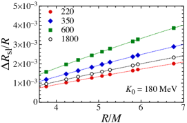
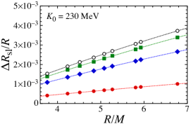
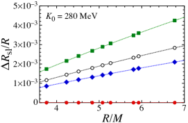
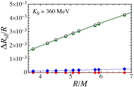
Figure 7: Same as Fig. 1, but for the ratio of the thickness of the phase composed of slab-like nuclei to the star’s radius. The dotted lines denote the fitting formula given by Eq. (32).

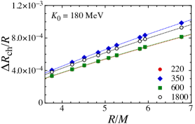
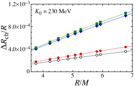
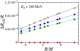
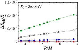
Figure 8: Same as Fig. 1, but for the ratio of the thickness of the phase composed of cylindrical-hole nuclei to the star’s radius. The dotted lines denote the fitting formula given by Eq. (33).

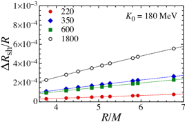
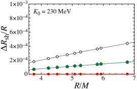
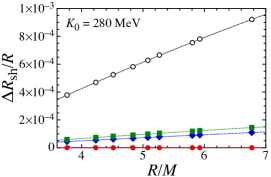
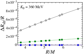
Figure 9: Same as Fig. 1, but for the ratio of the thickness of the phase composed of spherical-hole nuclei to the star’s radius. The dotted lines denote the fitting formula given by Eq. (34).

Table 3: The optimized coefficients in Eq. (32).

$K_{0}$ (MeV)	$L$ (MeV)	$\alpha_{1}^{\rm sl}$	$\alpha_{s}^{\rm sl}$	$\alpha_{3}^{\rm sl}$
180	5.7	$1.502\times 10^{-5}$	$6.138\times 10^{-4}$	$1.140\times 10^{-3}$
180	17.5	$2.432\times 10^{-5}$	$1.012\times 10^{-3}$	$1.881\times 10^{-3}$
180	31.0	$1.798\times 10^{-5}$	$7.561\times 10^{-4}$	$1.406\times 10^{-3}$
180	52.2	$1.211\times 10^{-5}$	$5.226\times 10^{-4}$	$9.740\times 10^{-4}$
230	7.6	$2.389\times 10^{-5}$	$9.801\times 10^{-4}$	$1.820\times 10^{-3}$
230	23.7	$2.113\times 10^{-5}$	$8.862\times 10^{-4}$	$1.647\times 10^{-3}$
230	42.6	$1.596\times 10^{-5}$	$6.896\times 10^{-4}$	$1.283\times 10^{-3}$
230	73.4	$5.723\times 10^{-6}$	$2.582\times 10^{-4}$	$4.819\times 10^{-4}$
280	9.6	$1.822\times 10^{-5}$	$7.460\times 10^{-4}$	$1.385\times 10^{-3}$
280	30.1	$2.568\times 10^{-5}$	$1.104\times 10^{-3}$	$2.051\times 10^{-3}$
280	54.9	$1.208\times 10^{-5}$	$5.399\times 10^{-4}$	$1.005\times 10^{-3}$
280	97.5	$0.0$	$0.0$	$0.0$
360	12.8	$2.691\times 10^{-5}$	$1.114\times 10^{-3}$	$2.068\times 10^{-3}$
360	40.9	$2.418\times 10^{-5}$	$1.079\times 10^{-3}$	$2.005\times 10^{-3}$
360	76.4	$1.660\times 10^{-6}$	$6.874\times 10^{-5}$	$1.279\times 10^{-4}$
360	146.1	$0.0$	$0.0$	$0.0$

Table 4: The optimized coefficients in Eq. (33).

$K_{0}$ (MeV)	$L$ (MeV)	$\alpha_{1}^{\rm ch}$	$\alpha_{s}^{\rm ch}$	$\alpha_{3}^{\rm ch}$
180	5.7	$5.827\times 10^{-6}$	$2.430\times 10^{-4}$	$4.510\times 10^{-4}$
180	17.5	$5.002\times 10^{-6}$	$2.123\times 10^{-4}$	$3.942\times 10^{-4}$
180	31.0	$6.025\times 10^{-6}$	$2.567\times 10^{-4}$	$4.771\times 10^{-4}$
180	52.2	$4.837\times 10^{-6}$	$2.102\times 10^{-4}$	$3.916\times 10^{-4}$
230	7.6	$2.244\times 10^{-6}$	$9.401\times 10^{-5}$	$1.744\times 10^{-4}$
230	23.7	$6.347\times 10^{-6}$	$2.710\times 10^{-4}$	$5.032\times 10^{-4}$
230	42.6	$5.886\times 10^{-6}$	$2.575\times 10^{-4}$	$4.787\times 10^{-4}$
230	73.4	$2.494\times 10^{-6}$	$1.129\times 10^{-4}$	$2.107\times 10^{-4}$
280	9.6	$6.487\times 10^{-6}$	$2.706\times 10^{-4}$	$5.023\times 10^{-4}$
280	30.1	$4.079\times 10^{-6}$	$1.789\times 10^{-4}$	$3.321\times 10^{-4}$
280	54.9	$4.766\times 10^{-6}$	$2.152\times 10^{-4}$	$4.002\times 10^{-4}$
280	97.5	$0.0$	$0.0$	$0.0$
360	12.8	$2.146\times 10^{-6}$	$9.086\times 10^{-5}$	$1.685\times 10^{-4}$
360	40.9	$4.630\times 10^{-6}$	$2.112\times 10^{-4}$	$3.918\times 10^{-4}$
360	76.4	$4.882\times 10^{-7}$	$2.024\times 10^{-5}$	$3.763\times 10^{-5}$
360	146.1	$0.0$	$0.0$	$0.0$

Table 5: The optimized coefficients in Eq. (34).

$K_{0}$ (MeV)	$L$ (MeV)	$\alpha_{1}^{\rm sh}$	$\alpha_{s}^{\rm sh}$	$\alpha_{3}^{\rm sh}$
180	5.7	$3.435\times 10^{-6}$	$1.449\times 10^{-4}$	$2.689\times 10^{-4}$
180	17.5	$1.395\times 10^{-6}$	$5.952\times 10^{-5}$	$1.105\times 10^{-4}$
180	31.0	$1.610\times 10^{-6}$	$6.892\times 10^{-5}$	$1.281\times 10^{-4}$
180	52.2	$4.609\times 10^{-7}$	$2.008\times 10^{-5}$	$3.740\times 10^{-5}$
230	7.6	$2.718\times 10^{-6}$	$1.146\times 10^{-4}$	$2.125\times 10^{-4}$
230	23.7	$1.035\times 10^{-6}$	$4.446\times 10^{-5}$	$8.253\times 10^{-5}$
230	42.6	$1.020\times 10^{-6}$	$4.479\times 10^{-5}$	$8.326\times 10^{-5}$
230	73.4	$2.312\times 10^{-8}$	$1.048\times 10^{-6}$	$1.955\times 10^{-6}$
280	9.6	$5.688\times 10^{-6}$	$2.405\times 10^{-4}$	$4.462\times 10^{-4}$
280	30.1	$8.503\times 10^{-7}$	$3.744\times 10^{-5}$	$6.949\times 10^{-5}$
280	54.9	$6.170\times 10^{-7}$	$2.795\times 10^{-5}$	$5.198\times 10^{-5}$
280	97.5	$0.0$	$0.0$	$0.0$
360	12.8	$5.171\times 10^{-6}$	$2.205\times 10^{-4}$	$4.091\times 10^{-4}$
360	40.9	$8.349\times 10^{-7}$	$3.825\times 10^{-5}$	$7.096\times 10^{-5}$
360	76.4	$0.0$	$0.0$	$0.0$
360	146.1	$0.0$	$0.0$	$0.0$

3.4 Crust thickness

We conclude this section by deriving a simple fitting formula for the ratio of the crust thickness to the star’s radius. Such derivation may well be possible even though $\Delta R_{\rm sl}/R$, $\Delta R_{\rm ch}/R$, and $\Delta R_{\rm sh}/R$ are difficult to express by a simple fitting formula. This is because the crust thickness, $\Delta R$, is dominated by the phase composed of spherical nuclei, of which the thickness has been parametrized above.

In Fig. 10, we plot the results for $\Delta R/R$ obtained for various EOS parameters as a function of $R/M$, which can be accurately expressed by

$$\frac{\Delta R}{R}=-\alpha_{1}\left(\frac{R}{M}\right)^{2}+\alpha_{2}\left(\frac{R}{M}\right)-\alpha_{3},$$ (35)

where $\alpha_{1}$, $\alpha_{2}$, and $\alpha_{3}$ are positive dimensionless adjustable coefficients that depend on $(L,K_{0})$. It should be noticed that the dependence of $\Delta R/R$ on the EOS parameters is sufficiently weak that observations of $R/M$ would lead to deduction of $\Delta R/R$ within $\sim 10\%$ accuracy.

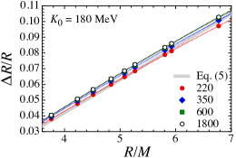
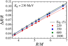
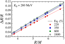
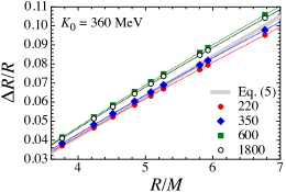
Figure 10: Same as Fig. 1, but for the ratio of the crust thickness to the star’s radius. The dotted lines denote the fitting formula given by Eq. (35), while the thick-solid line denotes the typical crust thickness given by Eq. (5).

The coefficients in Eq. (35) obtained by fitting for various sets of the EOS parameters are shown in Fig. 11 as a function of $L$. Then, we can successfully derive the fitting formula as

$$\alpha_{1} = \beta_{11}+\beta_{12}\left(\frac{L}{60\ {\rm MeV}}\right)+\beta_{13}\left(\frac{L}{60\ {\rm MeV}}\right)^{2},$$ (36)

$$\alpha_{2} = \beta_{21}+\beta_{22}\left(\frac{L}{60\ {\rm MeV}}\right)+\beta_{23}\left(\frac{L}{60\ {\rm MeV}}\right)^{2},$$ (37)

$$\alpha_{3} = \beta_{31}+\beta_{32}\left(\frac{L}{60\ {\rm MeV}}\right)+\beta_{33}\left(\frac{L}{60\ {\rm MeV}}\right)^{2},$$ (38)

where $\beta_{ij}$ with $i=1$, 2, 3 and $j=1$, 2, 3 are dimensionless adjustable coefficients that depend on $K_{0}$. In deriving these fitting formulas, we omit the results with $K_{0}=360$ MeV, which are difficult to fit as in the cases of $\Delta R_{\rm sp}/R$ and $\Delta R_{\rm cy}/R$.

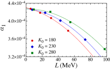
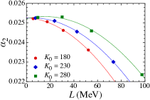
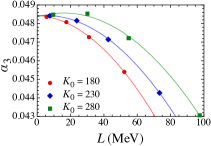
Figure 11: Same as Fig. 2, but for the coefficients in Eq. (35) and the fitting formula given by Eqs. (36)–(38).

Finally, in Fig. 12 we exhibit the normalized quantities $\bar{\beta}_{ij}$ of the coefficients in Eqs. (36)–(38) as a function of $K_{0}$, where $\bar{\beta}_{ij}$ is given by $\bar{\beta}_{11}=\beta_{11}\times 10^{4}$, $\bar{\beta}_{12}=\beta_{12}\times 10^{5}$, $\bar{\beta}_{13}=\beta_{13}\times 10^{5}$, $\bar{\beta}_{21}=\beta_{21}\times 10^{2}$, $\bar{\beta}_{22}=\beta_{22}\times 10^{4}$, $\bar{\beta}_{23}=\beta_{23}\times 10^{3}$, $\bar{\beta}_{31}=\beta_{31}\times 10^{2}$, $\bar{\beta}_{32}=\beta_{32}\times 10^{3}$, and $\bar{\beta}_{33}=\beta_{33}\times 10^{3}$. Again, the coefficients $\beta_{ij}$ can be expressed as a linear function of $K_{0}$ by

$$\beta_{11} = \left[4.3474-0.06256\left(\frac{K_{0}}{230\ {\rm MeV}}\right)\right]\times 10^{-4},$$ (39)

$$\beta_{12} = \left[-7.4004+6.2366\left(\frac{K_{0}}{230\ {\rm MeV}}\right)\right]\times 10^{-5},$$ (40)

$$\beta_{13} = \left[-4.4550+0.7337\left(\frac{K_{0}}{230\ {\rm MeV}}\right)\right]\times 10^{-5},$$ (41)

$$\beta_{21} = \left[2.5350-0.01058\left(\frac{K_{0}}{230\ {\rm MeV}}\right)\right]\times 10^{-2},$$ (42)

$$\beta_{22} = \left[-20.9930+23.9487\left(\frac{K_{0}}{230\ {\rm MeV}}\right)\right]\times 10^{-4},$$ (43)

$$\beta_{23} = \left[-2.5407+0.7880\left(\frac{K_{0}}{230\ {\rm MeV}}\right)\right]\times 10^{-3},$$ (44)

$$\beta_{31} = \left[4.8581-0.01794\left(\frac{K_{0}}{230\ {\rm MeV}}\right)\right]\times 10^{-2},$$ (45)

$$\beta_{32} = \left[-3.7203+4.3243\left(\frac{K_{0}}{230\ {\rm MeV}}\right)\right]\times 10^{-3},$$ (46)

$$\beta_{33} = \left[-4.8761+1.5884\left(\frac{K_{0}}{230\ {\rm MeV}}\right)\right]\times 10^{-3}.$$ (47)

Now, we obtain a complete set of the fitting formulas (35)–(47), which well reproduce the calculated values of $\Delta R/R$ for various combinations of $R/M$, $L$, and $K_{0}$. Note that applicability of these formulas is here again limited to the range of $180\,\,\raisebox{-3.44444pt}{$\stackrel{{\scriptstyle\textstyle<}}{{\sim}}$ }K_{0}\,\,\raisebox{-3.44444pt}{$\stackrel{{\scriptstyle\textstyle<}}{{\sim}}$ }280$ MeV.

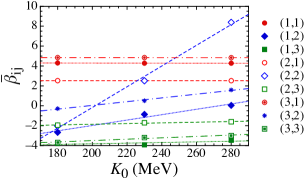
Figure 12: The normalized quantities $\bar{\beta}_{ij}$ of the coefficients in Eqs. (36)–(38) plotted as a function of $K_{0}$, where the labels of $(i,j)$ for $i=1$, 2, 3 and $j=1$, 2, 3 denote the subscript in $\bar{\beta}_{ij}$. The dotted lines denote the fitting formulas given by Eqs. (39)–(47).

4 Conclusion

We have constructed the fitting formulas for the thickness of the whole crust and the layers of the respective pasta phases in a manner that is dependent on the neutron star compactness $M/R$ and the EOS parameters $L$ and $K_{0}$. We find from the approximate form of the EOS [Eq. (1)] and the thickness [Eq. (2)] that the $L$ and $K_{0}$ dependence is much weaker than the $M/R$ for the whole crust and the SP phase, while being as strong for each of the pasta (C, S, CH, SH) phases. We remark that the known approximate dependence of the crust thickness on the compactness (e.g., Pethick & Ravenhall (1995)) is updated here by including the term of order $(M/R)^{2}$ in Eq. (35). The resultant fitting formulas would be useful in deducing the thickness of the whole crust and the layer of the SP phase from future accurate determinations of $M/R$ of X-ray bursters by LOFT and millisecond pulsars by NICER.

We thank K. Nakazato for useful discussion in the initial stage of the present study. This work was supported in part by Grants-in-Aid for Scientific Research on Innovative Areas through No. 15H00843 and No. 24105008 provided by MEXT, by Grant-in-Aid for Young Scientists (B) through No. 26800133 provided by JSPS, and by Grant-in-Aid for Scientific Research (C) through Grant No. 17K05458 provided by JSPS.

References

- Pulsar Group (2016) ATNF Pulsar Group, http://www.atnf.csiro.au
- Caplan et al. (2015) Caplan M. E., Schneider A. S., Horowitz C. J., Berry D. K., 2015, Phys. Rev. C, 91, 065802
- Dorso, Giménez Molinelli & López (2012) Dorso C. O., Giménez Molinelli P. A., López J. A., 2012, Phys. Rev. C, 86, 055805
- Gearheart et al. (2011) Gearheart M., Newton W. G., Hooker J., Li B. A., 2011, MNRAS, 418, 2343
- Haensel, Potekhin & Yakovlev (2007) Haensel P., Potekhin A. Y., Yakovlev D. G., Neutron Stars 1: Equation of State and Structure, Springer, New York.
- Horowitz et al. (2015) Horowitz C. J., Berry D. K., Briggs C. M., Caplan M. E., Cumming A., Schneider A. S., 2015, Phys. Rev. Lett., 114, 031102
- Hurley et al. (1999) Hurley K. et al., 1999, Nature, 397, L41
- Iida & Sato (1997) Iida K., Sato K., 1997, ApJ, 477, 294
- Iida & Oyamatsu (2014) Iida K., Oyamatsu K., 2014, Eur. Phys. J. A, 50, 42
- Khan & Margueron (2013) Khan E., Margueron J., 2013, Phys. Rev. C, 88, 034319
- Kouveliotou et al. (1998) Kouveliotou C. et al., 1998, Nature, 393, L235
- Lattimer (1981) Lattimer J. M., 1981, Annu. Rev. Nucl. Part. Sci., 31, 337
- Li (2017) Li B. A., 2017, arXiv:1701.03564
- Lorenz, Ravenhall & Pethick (1993) Lorenz C. P., Ravenhall D. G., Pethick C. J., 1993, Phys. Rev. Lett., 70, 379
- Newton et al. (2013) Newton W. G., Murphy K., Hooker J., Li B. A., 2013, ApJ, 779, L4
- Newton et al. (2014) Newton W. G., Hooker J., Gearheart M., Murphy K., Wen D. H., Fattoyev F. J., Li B. A., 2014, Eur. Phys. J. A, 50, 41
- Oyamatsu (1993) Oyamatsu K., 1993, Nucl. Phys. A, 561, 431
- Oyamatsu & Iida (2003) Oyamatsu K., Iida K., 2003, Prog. Theor. Phys., 109, 631
- Oyamatsu & Iida (2007) Oyamatsu K., Iida K., 2007, Phys. Rev. C, 75, 015801
- Passamonti & Pons (2016) Passamonti A., Pons J. A., 2016, MNRAS, 463, 1173
- Pethick & Ravenhall (1995) Pethick C. J., Ravenhall D. G., 1995, Annu. Rev. Nucl. Part. Sci. 45, 429
- Pons, Viganò & Rea (2013) Pons J. A., Viganò D., Rea N., 2013, Nature Phys., 9, 431
- Ravenhall & Pethick (1994) Ravenhall D. G., Pethick C. J., 1994, ApJ, 424, 846
- Schuetrumpf et al. (2014) Schuetrumpf B., Iida K., Maruhn J. A., Reinhard P.-G., 2014, Phys. Rev. C, 90, 055802
- Sébille, de la Mota & Figerou (2011) Sébille F., de la Mota V., Figerou S., 2011, Phys. Rev. C, 84, 055801
- Sotani (2011) Sotani H., 2011, MNRAS, 417, L70
- Sotani et al. (2012) Sotani H., Nakazato K., Iida K., Oyamatsu K., 2012, Phys. Rev. Lett., 108, 201101
- Sotani et al. (2013a) Sotani H., Nakazato K., Iida K., Oyamatsu K., 2013a, MNRAS, 428, L21
- Sotani et al. (2013b) Sotani H., Nakazato K., Iida K., Oyamatsu K., 2013b, MNRAS, 434, 2060
- Sotani (2014) Sotani H., 2014, Phys. Lett. B, 730, 166
- Sotani, Iida & Oyamatsu (2015) Sotani H., Iida K., Oyamatsu K., 2015, Phys. Rev. C, 91, 015805
- Sotani, Iida & Oyamatsu (2016) Sotani H., Iida K., Oyamatsu K., 2016, New Astron., 43, 80
- Sotani (2016) Sotani H., 2016, Phys. Rev. D, 93, 044059
- Sotani, Iida & Oyamatsu (2017) Sotani H., Iida K., Oyamatsu K., 2017, MNRAS, 464, 3101
- Steiner & Watts (2009) Steiner A. W., Watts A. L., 2009, Phys. Rev. Lett., 103, 181101
- Stone, Stone & Moszkowski (2014) Stone J. R., Stone N. J., Moszkowski S. A., 2014, Phys. Rev. C, 89, 044316
- Tsang et al. (2012) Tsang M. B. et al., 2012, Phys. Rev. C, 86, 015803
- Watanabe et al. (2003) Watanabe G., Sato K., Yasuoka K., Ebisuzaki T., 2003, Phys. Rev. C, 68, 035806
- Watts & Strohmayer (2006) Watts A. L., Strohmayer T. E., 2006, Adv. Space Res., 40, 1446
- Zdunik & Haensel (2011) Zdunik J. L., Haensel P., 2011, Astron. Astrophys., 530, A137
- Zdunik, Fortin & Haensel (2017) Zdunik J. L., Fortin M., Haensel P., 2017, Astron. Astrophys., 599 A119