Revenue Optimization with Approximate Bid Predictions

Abstract

In the context of advertising auctions, finding good reserve prices is a notoriously challenging learning problem. This is due to the heterogeneity of ad opportunity types, and the non-convexity of the objective function. In this work, we show how to reduce reserve price optimization to the standard setting of prediction under squared loss, a well understood problem in the learning community. We further bound the gap between the expected bid and revenue in terms of the average loss of the predictor. This is the first result that formally relates the revenue gained to the quality of a standard machine learned model.

1 Introduction

A crucial task for revenue optimization in auctions is setting a good reserve (or minimum) price. Set it too low, and the sale may yield little revenue, set it too high and there may not be anyone willing to buy the item. The celebrated work by Myerson (1981) shows how to optimally set reserves in second price auctions, provided the value distribution of each bidder is known.

In practice there are two challenges that make this problem significantly more complicated. First, the value distribution is never known directly; rather, the auctioneer can only observe samples drawn from it. Second, in the context of ad auctions, the items for sale (impressions) are heterogeneous, and there are literally trillions of different types of items being sold. It is therefore likely that a specific type of item has never been observed previously, and no information about its value is known.

A standard machine learning approach addressing the heterogeneity problem is to parametrize each impression by a feature vector, with the underlying assumption that bids observed from auctions with similar features will be similar. In online advertising. these features encode, for instance, the ad size, whether it’s mobile or desktop, etc.

The question is, then, how to use the features to set a good reserve price for a particular ad opportunity. On the face of it, this sounds like a standard machine learning question—given a set of features, predict the value of the maximum bid. The difficulty comes from the shape of the loss function. Much of the machine learning literature is concerned with optimizing well behaved loss functions, such as squared loss, or hinge loss. The revenue function, on the other hand is non-continuous and strongly non-concave, making a direct attack a challenging proposition.

In this work we take a different approach and reduce the problem of finding good reserve prices to a prediction problem under the squared loss. In this way we can rely upon many widely available and scalable algorithms developed to minimize this objective. We proceed by using the predictor to define a judicious clustering of the data, and then compute the empirically maximizing reserve price for each group. Our reduction is simple and practical, and directly ties the revenue gained by the algorithm to the prediction error.

1.1 Related Work

Optimizing revenue in auctions has been a rich area of study, beginning with the seminal work of  Myerson (1981) who introduced optimal auction design. Follow up work by  Chawla et al. (2007) and  Hartline and Roughgarden (2009), among others, refined his results to increasingly more complex settings, taking into account multiple items, diverse demand functions, and weaker assumptions on the shape of the value distributions.

Most of the classical literature on revenue optimization focuses on the design of optimal auctions when the bidding distribution of buyers is known. More recent work has considered the computational and information theoretic challenges in learning optimal auctions from data. A long line of work (Cole and Roughgarden, 2015; Devanur et al., 2016; Dhangwatnotai et al., 2015; Morgenstern and Roughgarden, 2015, 2016) analyzes the sample complexity of designing optimal auctions. The main contribution of this direction is to show that under fairly general bidding scenarios, a near-optimal auction can be designed knowing only a polynomial number of samples from bidders’ valuations. Other authors,  (Leme et al., 2016; Roughgarden and Wang, 2016) have focused on the computational complexity of finding optimal reserve prices from samples, showing that even for simple mechanisms the problem is often NP-hard to solve directly.

Another well studied approach to data-driven revenue optimization is that of online learning. Here, auctions occur one at a time, and the learning algorithm must compute prices as a function of the history of the algorithm. These algorithms generally make no distributional assumptions and measure their performance in terms of regret: the difference between the algorithm’s performance and the performance of the best fixed reserve price in hindsight. Kleinberg and Leighton (2003) developed an online revenue optimization algorithm for posted-price auctions that achieves low regret. Their work was later extended to second-price auctions by Cesa-Bianchi et al. (2015).

A natural approach in both of these settings is to attempt to predict an optimal reserve price, equivalently the highest bid submitted by any of the buyers. While the problem of learning this reserve price is well understood for the simplistic model of buyers with i.i.d. valuations (Cesa-Bianchi et al., 2015; Devanur et al., 2016; Kleinberg and Leighton, 2003), the problem becomes much more challenging in practice, when the valuations of a buyer also depend on features associated with the ad opportunity (for instance user demographics, and publisher information).

This problem is not nearly as well understood as its i.i.d. counterpart. Mohri and Medina (2014) provide learning guarantees and an algorithm based on DC programming to optimize revenue in second-price auctions with reserve. The proposed algorithm, however, does not easily scale to large auction data sets as each iteration involves solving a convex optimization problem. A smoother version of this algorithm is given by (Rudolph et al., 2016). However, being a highly non-convex problem, neither algorithm provides a guarantee on the revenue attainable by the algorithm’s output. Devanur et al. (2016) give sample complexity bounds on the design of optimal auctions with side information. However, the authors consider only cases where this side information is given by $\sigma\in[0,1]$. More importantly, their proposed algorithm only works under the unverifiable assumption that the conditional distributions of bids given $\sigma$ satisfy stochastic dominance.

Our results. We show that given a predictor of the bid with squared loss of $\eta^{2}$, we can construct a reserve function $r$ that extracts all but $g(\eta)$ revenue, for a simple increasing function $g$. (See Theorem  2 for the exact statement.) To the best of our knowledge, this is the first result that ties the revenue one can achieve directly to the quality of a standard prediction task. Our algorithm for computing $r$ is scalable, practical, and efficient.

Along the way we show what kinds of distributions are amenable to revenue optimization via reserve prices. We prove that when bids are drawn i.i.d. from a distribution $F$, the ratio between the mean bid and the revenue extracted with the optimum monopoly reserve scales as $O(\log{\bf Var}(F))$ – Theorem  5. This result refines the $\log h$ bound derived by  Goldberg et al. (2001), and formalizes the intuition that reserve prices are more successful for low variance distributions.

2 Setup

We consider a repeated posted price auction setup where every auction is parametrized by a feature vector $x\in\mathcal{X}$ and a bid $b\in[0,1]$. Let $D$ be a distribution over $\mathcal{X}\times[0,1]$. Let $h\colon\mathcal{X}\to[0,1]$, be a bid prediction function and denote by $\eta^{2}$ the squared loss incurred by $h$:

$$\operatorname*{\mathbb{E}}[(h(x)-b)^{2}]=\eta^{2}.$$

We assume $h$ is given, and make no assumption on the structure of $h$ or how it is obtained. Notice that while the existence of such $h$ is not guaranteed for all values of $\eta$, using historical data one could use one of multiple readily available regression algorithms to find the best hypothesis $h$.

Let $\mathcal{S}=\big{(}(x_{1},b_{1}),\ldots,(x_{m},b_{m})\big{)}\sim D$ be a set of $m$ i.i.d. samples drawn from $D$ and denote by $\mathcal{S}_{\mathcal{X}}=(x_{1},\ldots,x_{m})$ its projection on $\mathcal{X}$. Given a price $p$ let $\text{Rev}(p,b)=p\mathds{1}_{b\geq p}$ denote the revenue obtained when the bidder bids $b$. For a reserve price function ${r}\colon\mathcal{X}\to[0,1]$ we let:

$$\mathcal{R}({r})=\operatorname*{\mathbb{E}}_{(x,b)\sim D}\big{[}\text{Rev}({r}(x),b)\big{]}\quad\text{and}\quad\widehat{\mathcal{R}}({r})=\frac{1}{m}\sum_{(x,b)\in\mathcal{S}}\text{Rev}(r(x),b)$$

denote the expected and empirical revenue of reserve price function ${r}$.

We also let $B=\operatorname*{\mathbb{E}}[b]$, $\widehat{B}=\frac{1}{m}\sum_{i=1}^{m}b_{i}$ denote the population and empirical mean bid, and $S({r})=B-\mathcal{R}({r})$, $\widehat{S}({r})=\widehat{B}-\widehat{\mathcal{R}}(r)$ denote the expected and empirical separation between bid values and the revenue. Notice that for a given reserve price function ${r}$, $S({r})$ corresponds to revenue left on the table. Our goal is, given $\mathcal{S}$ and $h$, to find a function ${r}$ that maximizes $\mathcal{R}({r})$ or equivalently minimizes $S({r})$.

2.1 Generalization Error

Note that in our set up we are only given samples from the distribution, $D$, but aim to maximize the expected revenue. Understanding the difference between the empirical performance of an algorithm and its expected performance, also known as the generalization error, is a key tenet of learning theory.

At a high level, the generalization error is a function of the training set size: larger training sets lead to smaller generalization error; and the inherent complexity of the learning algorithm: simple rules such as linear classifiers generalize better than more complex ones.

In this paper we characterize the complexity of a class $G$ of functions by its growth function $\Pi$. The growth function corresponds to the maximum number of binary labelings that can be obtained by $G$ over all possible samples $\mathcal{S}_{\mathcal{X}}$. It is closely related to the VC-dimension when $G$ takes values in $\{0,1\}$ and to the pseudo-dimension (Morgenstern and Roughgarden, 2015; Mohri et al., 2012) when $G$ takes values in $\mathbb{R}$.

We can give a bound on the generalization error associated with minimizing the empirical separation over a class of functions $G$. The following theorem is an adaptation of Theorem 1 of (Mohri and Medina, 2014) to our particular setup.

Theorem 1.

Let $\delta>0$, with probability at least $1-\delta$ over the choice of the sample $\mathcal{S}$ the following bound holds uniformly for $r\in G$

$$S({r})\leq\widehat{S}({r})+2\sqrt{\frac{\log 1/\delta}{2m}}+4\sqrt{\frac{2\log(\Pi(G,m))}{m}}.$$ (1)

Therefore, in order to minimize the expected separation $S({r})$ it suffices to minimize the empirical separation $\widehat{S}({r})$ over a class of functions $G$ whose growth function scales polynomially in $m$.

3 Warmup

In order to better understand the problem at hand, we begin by introducing a straightforward mechanism for transforming the hypothesis function $h$ to a reserve price function ${r}$ with guarantees on its achievable revenue.

Lemma 1.

Let ${r}\colon\mathcal{X}\to[0,1]$ be defined by ${r}(x):=\max(h(x)-\eta^{2/3},0)$. The function ${r}$ then satisfies $S({r})\leq\eta^{1/2}+2\eta^{2/3}.$

The proof is a simple application of Jensen’s and Markov’s inequalities and it is deferred to Appendix B.

This surprisingly simple algorithm shows there are ways to obtain revenue guarantees from a simple regressor. To the best of our knowledge these is the first guarantee of its kind. The reader may be curious about the choice of $\eta^{2/3}$ as the offset in our reserve price function. We will show that the dependence on $\eta^{2/3}$ is not a simple artifact of our analysis, but a cost inherent to the problem of revenue optimization.

Moreover, observe that this simple algorithm fixes a static offset, and does not make a distinction between those parts of the feature space, where the algorithm makes a low error, and those where the error is relatively high. By contrast our proposed algorithm partitions the space appropriately and calculates a different reserve for each partition. More importantly we will provide a data dependent bound on the performance of our algorithm that only in the worst case scenario behaves like $\eta^{2/3}$.

4 Results Overview

In principle to maximize revenue we need to find a class of functions $G$ with small complexity, but that contains a function which approximately minimizes the empirical separation. The challenge comes from the fact that the revenue function, Rev, is not continuous and highly non-concave—a small change in the price, $p$, may lead to very large changes in revenue. This is the main reason why simply using the predictor $h(x)$ as a proxy for a reserve function is a poor choice, even if its average error, $\eta^{2}$ is small. For example a function $h$, that is just as likely to over-predict by $\eta$ as to under predict by $\eta$ will have very small error, but lead to $0$ revenue in half the cases.

A solution on the other end of the spectrum would simply memorize the optimum prices from the sample $\mathcal{S}$, setting $r(x_{i})=b_{i}$. While this leads to optimal empirical revenue, a function class $G$ containing r would satisfy $\Pi(G,m)=2^{m}$, making the bound of Theorem 1 vacuous.

In this work we introduce a family $G(h,k)$ of classes parameterized by $k\in\mathbb{N}$. This family admits an approximate minimizer that can be computed in polynomial time, has low generalization error, and achieves provable guarantees to the overall revenue.

More precisely, we show that given $\mathcal{S}$, and a hypothesis $h$ with expected squared loss of $\eta^{2}$:

• For every $k\geq 1$ there exists a set of functions $G(h,k)$ such that $\Pi(G(h,k),m)=O(m^{2k})$.

• For every $k\geq 1$, there is a polynomial time algorithm that outputs ${r}_{k}\in G(h,k)$ such that in the worst case scenario $\widehat{S}({r}_{k})$ is bounded by $O(\frac{1}{k^{2/3}}+\eta^{2/3}+\frac{1}{m^{1/6}})$.

Effectively, we show how to transform any classifier $h$ with low squared loss, $\eta^{2}$, to a reserve price predictor that recovers all but $O(\eta^{2/3})$ revenue in expectation.

4.1 Algorithm Description

In this section we give an overview of the algorithm that uses both the predictor $h$ and the set of samples in $\mathcal{S}$ to develop a pricing function ${r}$. Our approach has two steps. First we partition the set of feasible prices, $0\leq p\leq 1,$ into $k$ partitions, $C_{1},C_{2},\ldots,C_{k}$. The exact boundaries between partitions depend on the samples $\mathcal{S}$ and their predicted values, as given by $h$. For each partition we find the price that maximizes the empirical revenue in the partition. We let ${r}(x)$ return the empirically optimum price in the partition that contains $h(x)$.

For a more formal description, let $\mathcal{T}_{k}$ be the set of $k$-partitions of the interval $[0,1]$ that is:

$$\mathcal{T}_{k}=\{\mathbf{t}=(t_{0},t_{1},\ldots,t_{k-1},t_{k})\ |\ 0=t_{0}<\ldots<t_{k}=1\}.$$

We define $G(h,k)=\{x\mapsto\sum_{j=0}^{k-1}r_{i}\mathds{1}_{t_{j}\leq h(x)<t_{j+1}}\ |\ r_{j}\in[t_{i},t_{j+1}]\;\text{and}\;\mathbf{t}\in\mathcal{T}_{k}\}$. A function in $G(h,k)$ chooses $k$ level sets of $h$ and $k$ reserve prices. Given $x$, price $r_{j}$ is chosen if $x$ falls on the $j$-th level set.

It remains to define the function $r_{k}\in G(h,k)$. Given a partition vector $\mathbf{t}\in\mathcal{T}_{k}$, let the partition $\mathcal{C}^{h}=\{C^{h}_{1},\ldots,C^{h}_{k}\}$ of $\mathcal{X}$ be given by $C^{h}_{j}=\{x\in\mathcal{X}|t_{j-1}<h(x)\leq t_{j}\}$. Let $m_{j}=|\mathcal{S}_{\mathcal{X}}\cap C^{h}_{j}|$ be the number of elements that fall into the $j$-th partition.

We define the predicted mean and variance of each group $C_{j}^{h}$ as

$$\mu^{h}_{j}=\frac{1}{m_{j}}\sum_{x_{i}\in C^{h}_{j}}h(x_{i})\qquad\text{and}\qquad(\sigma^{h}_{j})^{2}=\frac{1}{m_{j}}\sum_{x_{i}\in C^{h}_{j}}(h(x_{i})-\mu_{j})^{2}.$$

We are now ready to present algorithm RIC-$h$ for computing $r_{k}\in H_{k}$.

Reserve Inference from Clusters

  Compute $\mathbf{t}^{h}\in\mathcal{T}_{k}$ that minimizes $\frac{1}{m}\sum_{j=0}^{k-1}m_{j}\sigma^{h}_{j}$.

  Let $\mathcal{C}^{h}=C^{h}_{1},C^{h}_{2},\ldots,C^{h}_{k}$ be the induced partitions.

  For each $j\in 1,\ldots,k$, set $r_{j}=\max_{r}r\cdot|\{i|b_{i}\geq r\wedge x_{i}\in C^{h}_{j}\}|$.

  Return $x\mapsto\sum_{j=0}^{k-1}r_{j}\mathds{1}_{h(x)\in C^{h}_{j}}$.

Our main theorem states that the separation of $r_{k}$ is bounded by the cluster variance of $\mathcal{C}^{h}$. For a partition $\mathcal{C}=\{C_{1},\ldots,C_{k}\}$ of $\mathcal{X}$ let $\sigma_{j}$ denote the empirical variance of bids for auctions in $C_{j}$. We define the weighted empirical variance by:

$$\Phi(\mathcal{C})\colon=\sum_{j=1}^{k}\sqrt{\sum_{i,i^{\prime}:x_{i},x_{i^{\prime}}\in C_{k}}(b_{i}-b_{i^{\prime}})^{2}}=2\sum_{j=1}^{k}m_{j}\widehat{\sigma}_{j}$$ (2)

Theorem 2.

Let $\delta>0$ and let ${r}_{k}$ denote the output of Algorithm 4.1 then ${r}_{k}\in G(h,k)$ and with probability at least $1-\delta$ over the samples $\mathcal{S}$:

$$\widehat{S}({r}_{k})\leq(3\widehat{B})^{1/3}\Big{(}\frac{1}{2m}\Phi(\mathcal{C}^{h})\Big{)}\leq(3\widehat{B})^{1/3}\Big{(}\frac{1}{2k}+2\Big{(}\eta^{2}+\sqrt{\frac{\log 1/\delta}{2m}}\Big{)}^{1/2}\Bigg{)}^{2/3}.$$

Notice that our bound is data dependent and only in he worst case scenario it behaves like $\eta^{2/3}$. In general it could be much smaller.

We also show that the complexity of $G(h,k)$ admits a favorable bound. The proof is similar to that in (Morgenstern and Roughgarden, 2015); we include it in Appendix  E for completness.

Theorem 3.

The growth function of the class $G(h,k)$ can be bounded as: $\Pi(G(h,k),m)\leq\frac{m^{2k-1}}{k^{k}}.$

We can combine these results with Equation 1 and an easy bound on $\widehat{B}$ in terms of $B$ to conclude:

Corollary 1.

Let $\delta>0$ and let ${r}_{k}$ denote the output of Algorithm 4.1 then ${r}_{k}\in G(h,k)$ and with probability at least $1-\delta$ over the samples $\mathcal{S}$:

$$S({r}_{k})\leq(3\widehat{B})^{1/3}\Big{(}\frac{\Phi(\mathcal{C}^{h})}{2m}\Big{)}+O\Big{(}\sqrt{\frac{k\log m}{m}}\Big{)}\leq(12B\eta^{2})^{1/3}+O\Big{(}\frac{1}{k^{2/3}}+\Big{(}\frac{\log 1/\delta}{2m}\Big{)}^{1/6}\!\!\!+\!\sqrt{\frac{k\log m}{m}}\Big{)}.$$

Since $B\in[0,1]$, this implies that when $k=\Theta(m^{3/7})$, the separation is bounded by $2.28\eta^{2/3}$ plus additional error factors that go to 0 with the number of samples, $m$, as $\tilde{O}(m^{-\nicefrac{{2}}{{7}}}).$

5 Bounding Separation

In this section we prove the main bound motivating our algorithm. This bound relates the variance of the bid distribution and the maximum revenue that can be extracted when a buyer’s bids follow such distribution. It formally shows what makes a distribution amenable to revenue optimization.

To gain intuition for the kind of bound we are striving for, consider a bid distribution $F$. If the variance of $F$ is $0$, that is $F$ is a point mass at some value $v$, then setting a reserve price to $v$ leads to no separation. On the other hand, consider the equal revenue distribution, with $F(x)=1-\nicefrac{{1}}{{x}}$. Here any reserve price leads to revenue of $1$. However, the distribution has unbounded expected bid and variance, so it is not too surprising that more revenue cannot be extracted. We make this connection precise, showing that after setting the optimal reserve price, the separation can be bounded by a function of the variance of the distribution.

Given any bid distribution $F$ over $[0,1]$ we denote by $G(r)=1-\lim_{r^{\prime}\to r^{-}}F(r^{\prime})$ the probability that a bid is greater than or equal to $r$. Finally, we will let $R=\max_{r}rG(r)$ denote the maximum revenue achievable when facing a bidder whose bids are drawn from distribution $F$. As before we denote by $B=\operatorname*{\mathbb{E}}_{b\sim F}[b]$ the mean bid and by $S=B-R$ the expected separation of distribution $F$.

Theorem 4.

Let $\sigma^{2}$ denote the variance of $F$. Then $\sigma^{2}\geq 2R^{2}e^{\frac{S}{R}}-B^{2}-R^{2}.$

The proof of this theorem is highly technical and we present it in Appendix A.

Corollary 2.

The following bound holds for any distribution F: $S\leq(3R)^{1/3}\sigma^{2/3}\leq(3B)^{1/3}\sigma^{2/3}$

The proof of this corollary follows immediately by an application of Taylor’s theorem to the bound of Theorem 4. It is also easy to show that this bound is tight (see Appendix  D).

5.1 Approximating Maximum Revenue

In their seminal work Goldberg et al. (2001) showed that when faced with a bidder drawing values distribution $F$ on $[1,M]$ with mean $B$, an auctioneer setting the optimum monopoly reserve would recover at least $\Omega(B/\log M)$ revenue. We show how to adapt the result of Theorem 4 to refine this approximation ratio as a function of the variance of $F$. We defer the proof to Appendix B.

Theorem 5.

For any distribution $F$ with mean $B$ and variance $\sigma^{2}$, the maximum revenue with monopoly reserves, $R$, satisfies: $\frac{B}{R}\leq 4.78+2\log\big{(}1+\frac{\sigma^{2}}{B^{2}}\big{)}$

Note that since $\sigma^{2}\leq M^{2}$ this always leads to a tighter bound on the revenue.

5.2 Partition of $\mathcal{X}$

Corollary 2 suggests clustering points in such a way that the variance of the bids in each cluster is minimized. Given a partition $\mathcal{C}=\{C_{1},\ldots,C_{k}\}$ of $\mathcal{X}$ we denote by $m_{j}=|\mathcal{S}_{\mathcal{X}}\cup C_{j}|$, $\widehat{B}_{j}=\frac{1}{m_{j}}\sum_{i:x_{i}\in C_{j}}b_{i}$, $\widehat{\sigma}_{j}^{2}=\frac{1}{m_{j}}\sum_{i:x_{i}\in C_{j}}(b_{i}-\widehat{B}_{j})^{2}$. Let also $r_{j}=\arg\!\max_{p>0}p|\{b_{i}>p|x_{i}\in C_{j}\}|$ and $\widehat{R}_{j}=r_{j}|\{b_{i}>r_{j}|x_{i}\in C_{j}\}|$.

Lemma 2.

Let $r(x)=\sum_{j=1}^{k}r_{j}\mathds{1}_{x\in C_{j}}$ then $\widehat{S}(r)\leq\Big{(}3\widehat{B}\Big{)}^{1/3}\Big{(}\frac{1}{m}\sum_{j=1}^{k}m_{j}\widehat{\sigma}_{j}\Big{)}^{2/3}=\Big{(}3\widehat{B}\Big{)}^{1/3}\Big{(}\frac{1}{2m}\Phi(\mathcal{C})\Big{)}.$

Proof.

Let $\widehat{S}_{j}=\widehat{B}_{j}\!\!-\!\!\widehat{R}_{j}$, Corollary 2 applied to the empirical bid distribution in $C_{j}$ yields $\widehat{S}_{j}\!\!\leq\!\!(3\widehat{B}_{j})^{1/3}\widehat{\sigma}_{j}^{2/3}$. Multiplying by $\frac{m_{j}}{m}$, summing over all clusters and using Hölder’s inequality gives:

$$\widehat{S}(r)=\frac{1}{m}\sum_{j=1}^{k}m_{j}S_{j} \leq\frac{1}{m}\sum_{j=1}^{k}(3\widehat{B}_{j})^{1/3}\widehat{\sigma}_{j}^{2/3}m_{j}\leq\Big{(}\sum_{j=1}^{k}\frac{3m_{j}}{m}\widehat{B}_{j}\Big{)}^{1/3}\Big{(}\sum_{j=1}^{k}\frac{m_{j}}{m}\widehat{\sigma}_{j}\Big{)}^{2/3}.$$

∎

6 Clustering Algorithm

In view of Lemma 2 and since the quantity $\widehat{B}$ is fixed, we can find a function minimizing the expected separation by finding a partition of $\mathcal{X}$ that minimizes the weighted variance $\Phi(\mathcal{C})$ defined Section 4.1. From the definition of $\Phi$, this problem resembles a traditional $k$-means clustering problem with distance function $d(x_{i},x_{i^{\prime}})=(b_{i}-b_{i^{\prime}})^{2}$. Thus, one could use one of several clustering algorithms to solve it. Nevertheless, in order to allocate a new point $x\in\mathcal{X}$ to a cluster, we would require access to the bid $b$ which at evaluation time is unknown. Instead, we show how to utilize the predictions of $h$ to define an almost optimal clustering of $\mathcal{X}$.

For any partition $\mathcal{C}=\{C_{1},\ldots,C_{k}\}$ of $\mathcal{X}$ define

$$\Phi_{h}(\mathcal{C})=\sum_{j=1}^{k}\sqrt{\sum_{i,i^{\prime}:x_{i},x_{i^{\prime}}\in C_{k}}(h(x_{i})-h(x_{i^{\prime}}))^{2}}.$$

Notice that $\frac{1}{2m}\Phi_{h}(C)$ is the function minimized by Algorithm 4.1. The following lemma, proved in Appendix B, bounds the cluster variance achieved by clustering bids according to their predictions.

Lemma 3.

Let $h$ be a function such that $\frac{1}{m}\sum_{i=1}^{m}(h(x_{i})-b_{i})^{2}\leq\widehat{\eta}^{2}$, and let $\mathcal{C}^{*}$ denote the partition that minimizes $\Phi(\mathcal{C})$. If $\mathcal{C}^{h}$ minimizes $\Phi_{h}(\mathcal{C})$ then $\Phi(\mathcal{C}^{h})\leq\Phi(\mathcal{C}^{*})+4m\widehat{\eta}$.

Corollary 3.

Let $r_{k}$ be the output of Algorithm 4.1. If $\frac{1}{m}\sum_{j=1}^{m}(h(x_{i})-b_{i})^{2}\leq\widehat{\eta}^{2}$ then:

$$\widehat{S}(r_{k})\leq(3\widehat{B})^{1/3}\Big{(}\frac{1}{2m}\Phi(\mathcal{C}^{h})\Big{)}^{2/3}\leq(3\widehat{B})^{1/3}Big(\frac{1}{2m}\Phi(\mathcal{C}^{*})+2\widehat{\eta}\Big{)}^{2/3}.$$ (3)

Proof.

It is easy to see that the elements $C^{h}_{j}$ of $\mathcal{C}^{h}$ are of the form $C_{j}=\{x|t_{j}\leq h(x)\leq t_{j+1}\}$ for $\mathbf{t}\in\mathcal{T}_{k}$. Thus if $r_{k}$ is the hypothesis induced by the partition $\mathcal{C}^{h}$, then $r_{k}\in G(h,k)$. The result now follows by definition of $\Phi$ and lemmas 2 and 3. ∎

The proof of Theorem 2 is now straightforward. Define a partition $\mathcal{C}$ by $x_{i}\in C_{j}$ if $b_{i}\in\big{[}\frac{j-1}{k},\frac{j}{k}\big{]}$. Since $(b_{i}-b_{i^{\prime}})^{2}\leq\frac{1}{k^{2}}$ for $b_{i},b_{i^{\prime}}\in C_{j}$ we have

$$\Phi(\mathcal{C})\leq\sum_{j=1}^{k}\sqrt{\frac{m_{j}^{2}}{k^{2}}}=\frac{m}{k}.$$ (4)

Furthermore since $\operatorname*{\mathbb{E}}[(h(x)-b)^{2}]\leq\eta^{2}$, Hoeffding’s inequality implies that with probability $1-\delta$:

$$\frac{1}{m}\sum_{i=1}^{m}(h(x_{i})-b_{i})^{2}\leq\Big{(}\eta^{2}+\sqrt{\frac{\log 1/\delta}{2m}}\Big{)}.$$ (5)

In view of inequalities (4) and (5) as well as Corollary 3 we have:

$$\widehat{S}(r_{k})\leq(3\widehat{B})^{1/3}\Bigg{(}\frac{1}{2m}\Phi(\mathcal{C})+2\Big{(}\eta^{2}+\sqrt{\frac{\log 1/\delta}{2m}}\Big{)}^{1/2}\Bigg{)}^{2/3}\leq(3\widehat{B})^{1/3}\Big{(}\frac{1}{2k}+2\Big{(}\eta^{2}+\sqrt{\frac{\log 1/\delta}{2m}}\Big{)}^{1/2}\Bigg{)}^{2/3}$$

This completes the proof of the main result. To implement the algorithm, note that the problem of minimizing $\Phi_{h}(C)$ reduces to finding a partition $\mathbf{t}\in\mathcal{T}_{k}$ such that the sum of the variances within the partitions is minimized. It is clear that it suffices to consider points $t_{j}$ in the set $\mathcal{B}=\{h(x_{1}),\ldots,h(x_{m})\}$. With this observation, a simple dynamic program leads to a polynomial time algorithm with an $O(km^{2})$ running time (see Appendix C).

7 Experiments

We now compare the performance of our algorithm against the following baselines:

1. The offset algorithm presented in Section 3, where instead of using the theoretical offset $\eta^{2/3}$ we find the optimal $t$ maximizing the empirical revenue $\sum_{i=1}^{m}\big{(}h(x_{i})-t)\mathds{1}_{h(x_{i})-t\leq b_{i}}$.

2. The DC algorithm introduced by Mohri and Medina (2014), which represents the state of the art in learning a revenue optimal reserve price.

Synthetic data. We begin by running experiments on synthetic data to demonstrate the regimes where each algorithm excels. We generate feature vectors $\mathbf{x}_{i}\in\mathbb{R}^{10}$ with coordinates sampled from a mixture of lognormal distributions with means $\mu_{1}=0$, $\mu_{2}=1$, variance $\sigma_{1}=\sigma_{2}=0.5$ and mixture parameter $p=0.5$. Let $\mathbf{1}\in\mathbb{R}^{d}$ denote the vector with entries set to $1$. Bids are generated according to two different scenarios:

• Bids $b_{i}$ generated according to $b_{i}=\max(\mathbf{x}_{i}^{\top}\mathbf{1}+\beta_{i},0)$ where $\beta_{i}$ is a Gaussian random variable with mean $0$, and standard deviation $\sigma\in\{0.01,0.1,1.0,2.0,4.0\}$.

• Bids $b_{i}$ generated according to the following rule: let $s_{i}=\max(\mathbf{x}_{i}^{\top}\mathbf{1}+\beta_{i},0)$ if $s_{i}>30$ then $b_{i}=40+\alpha_{i}$ otherwise $b_{i}=s_{i}$. Here $\alpha_{i}$ has the same distribution as $\beta_{i}$.

The linear scenario demonstrates what happens when we have a good estimate of the bids. The bimodal scenario models a buyer, which for the most part will bid as a continuous function of features but that is interested in a particular set of objects (for instance retargeting buyers in online advertisement) for which she is willing to pay a much higher price.

For each experiment we generated a training dataset $\mathcal{S}_{train}$, a holdout set $\mathcal{S}_{holdout}$ and a test set $\mathcal{S}_{test}$ each with 16,000 examples. The function $h$ used by RIC-$h$ and the offset algorithm is found by training a linear regressor over $\mathcal{S}_{train}$. For efficiency, we ran RIC-$h$ algorithm on quantizations of predictions $h(x_{i})$. Quantized predictions belong to one of 1000 buckets over the interval $[0,50]$.

Finally, the choice of hyperparameters $\gamma$ for the Lipchitz loss and $k$ for the clustering algorithm was done by selecting the best performing parameter over the holdout set. Following the suggestions in (Mohri and Medina, 2014) we chose $\gamma\in\{0.001,0.01,0.1,1.0\}$ and $k\in\{2,4,\ldots,24\}$.

Figure 1(a),(b) shows the average revenue of the three approaches across 20 replicas of the experiment as a function of the log of $\sigma$. Revenue is normalized so that the DC algorithm revenue is $1.0$ when $\sigma=0.01$. The error bars at one standard deviation are indistinguishable in the plot. It is not surprising to see that in the linear scenario, the DC algorithm of (Mohri and Medina, 2014) and the offset algorithm outperform RIC-$h$ under low noise conditions. Both algorithms will recover a solution close to the true weight vector $\mathbf{1}$. In this case the offset is minimal, thus recovering virtually all revenue. On the other hand, even if we set the optimal reserve price for every cluster, the inherent variance of each cluster makes us leave some revenue on the table. Nevertheless, notice that as the noise increases all three algorithms seem to achieve the same revenue. This is due to the fact that the variance in each cluster is comparable with the error in the prediction function $h$.

The results are reversed for the bimodal scenario where RIC-$h$ outperforms both algorithms under low noise. This is due to the fact that RIC-$h$ recovers virtually all revenue obtained from high bids while the offset and DC algorithms must set conservative prices to avoid losing revenue from lower bids.

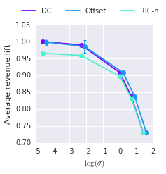
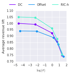
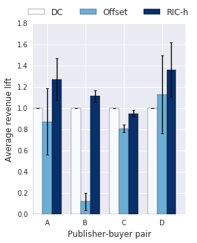
(a)	(b)	(c)

Figure 1: (a) Mean revenue of the three algorithms on the linear scenario. (b) Mean revenue of the three algorithms on the bimodal scenario. (c) Mean revenue on auction data.

Auction data. In practice, however, neither of the synthetic regimes is fully representative of the bidding patterns. In order to fully evaluate RIC-$h$, we collected auction bid data from AdExchange for 4 different publisher-advertiser pairs. For each pair we sampled 100,000 examples with a set of discrete and continuous features. The final feature vectors are in $\mathbb{R}^{d}$ for $d\in[100,200]$ depending on the publisher-buyer pair. For each experiment, we extract a random training sample of 20,0000 points as well as a holdout and test sample. We repeated this experiment 20 times and present the results on Figure 1 (c) where we have normalized the data so that the performance of the DC algorithm is always 1. The error bars represent one standard deviation from the mean revenue lift. Notice that our proposed algorithm achieves on average up to $30\%$ improvement over the DC algorithm. Moreover, the simple offset strategy never outperforms the clustering algorithm, and in some cases achieves significantly less revenue.

8 Conclusion

We provided a simple, scalable reduction of the problem of revenue optimization with side information to the well studied problem of minimizing the squared loss. Our reduction provides the first polynomial time algoritm with a quantifiable bound on the achieved revenue. In the analysis of our algorithm we also provided the first variance dependent lower bound on the revenue attained by setting optimal monopoly prices. Finally, we provided extensive empirical evidence of the advantages of RIC-$h$ over the current state of theart.

Appendix A Proof of Theorem 4

Recall that given any bid distribution $F$ over $[0,1]$ we denote by $G(r)=1-\lim_{r^{\prime}\to r^{-}}F(r^{\prime})$ the probability that a bid is greater than or equal to $r$. Let $\mathsf{x}(q)=\sup\{x|G(x)\geq q\}$ denote the pseudo-inverse of $G$. Notice in particular that when $G$ is strictly decreasing then $\mathsf{x}=G^{-1}$. When it is clear from context we will refer to a distribution indistinctly by $F$, $G$ or $\mathsf{x}$.

We will use the following expressions for the expected bid and second moment of a distribution.

Lemma 4.

The expected bid and second moments of any distribution $F$ are given respectively by:

$$B=\int_{0}^{1}\mathsf{x}(q)dq\quad\text{and}\quad s^{2}=\int_{0}^{1}\mathsf{x}(q)^{2}dq.$$

Proof.

We show the result only for the mean as the proof for the second moment is similar. It is well known that for a positive random variable, the mean can be expressed as:

$$B=\int_{0}^{\infty}G(x)dx=\int_{0}^{\infty}\int_{0}^{G(x)}dqdx=\int_{D}dqdx.$$

where $D=\{(x,q)\ |\ x>0\;\text{and}\;q\leq G(x)\}$. Let $D^{\prime}=\{(x,q)\ |\ 0\leq q\leq 1\;\text{and}\;x\leq\mathsf{x}(q)\}$. It is immediate that $D\subset D^{\prime}$ as $q\leq G(x)$ implies by definition that $x\leq\mathsf{x}(q)$. We can thus decompose the above integral as:

$$\int_{D}dqdx=\int_{D^{\prime}}dqdx-\int_{D^{\prime}-D}dqdx.$$

The proof will be complete by showing that $D^{\prime}-D$ has Lebesgue measure $0$. Indeed, in that case the above expression reduces to:

$$\int_{D^{\prime}}dqdx=\int_{0}^{1}\int_{0}^{\mathsf{x}(q)}dxdq=\int_{0}^{1}\mathsf{x}(q)dq.$$

Let us then characterize points $(x,q)\in D^{\prime}-D$. Notice that if $(x,q)\notin D$ then $G(x)<q$ but this again by definition implies $x\geq\mathsf{x}(q)$. If $(x,q)$ is also in $D^{\prime}$ then we must have $x=\mathsf{x}(q)$. From which we conclude that $\lim_{x^{\prime}\to x^{-}}G(x^{\prime})\geq q>G(x)$. Thus $(x,y)\in D^{\prime}-D$ implies that $x$ is a discontinuity of $G$. Finally, since $G$ is decreasing there can be at most a countable number of discontinuities and thus $D^{\prime}-D$ has measure 0. ∎

In order to show the bound of Theorem 4 holds, we consider the following optimization problem over the space of square integrable functions $L^{2}[0,1]$:

$$\min_{\mathsf{x}\in L_{2}[0,1]} \quad\frac{1}{2}\int_{0}^{1}\mathsf{x}^{2}(q)dq$$ (6)

s.t. $$\quad\int_{0}^{1}\mathsf{x}(q)=B\quad\text{and}\quad R\geq q\,\mathsf{x}(q)\;\forall q.$$

We show that the value of this optimization problem is greater than $\frac{1}{2}\big{(}2R^{2}e^{\frac{S}{R}}-R^{2}\big{)}$. Since any distribution $\mathsf{x}(q)$ achieving revenue $R$ and separation $S$ is feasible for (6) it follows that it must satisfy $\sigma^{2}=s^{2}-B^{2}\geq 2R^{2}e^{\frac{S}{R}}-B^{2}-R^{2}$.

Proposition 1.

The objective value of (6) is lower bounded by:

$$\frac{B^{2}}{2}+\max_{v\in L_{2}[0,1]:v\geq 0}-\frac{1}{2}\Big{(}\int_{0}^{1}(qv(q))^{2}-\Big{(}\int_{0}^{1}qv(q)\Big{)}^{2}\Big{)}+B\int_{0}^{1}qv(q)-R\int_{0}^{1}v(q).$$ (7)

Proof.

For any $\lambda\in\mathbb{R}$ and $v\in L_{2}[0,1]$ define the Lagrangian

$$L(x,\lambda,v)=\frac{1}{2}\int_{0}^{1}\mathsf{x}(q)^{2}-\lambda\int_{0}^{1}\mathsf{x}(q)+\lambda B+\int_{0}^{1}v(q)(q\,\mathsf{x}(q)-R).$$

It is immediate to see that optimization problem (6) is equivalent to

$$\min_{x\in L_{2}[0,1]}\max_{\lambda\in\mathbb{R},v\geq 0}L(x,\lambda,v)\geq\max_{\lambda\in\mathbb{R},v\geq 0}\min_{x\in L_{2}[0,1]}L(x,\lambda,v).$$

By taking variational derivatives of the function $L$ with respect to $\mathsf{x}$ we see that the minimizing solution $\mathsf{x}(q)$ satisfies:

$$\mathsf{x}(q)=\lambda-qv(q).$$

Replacing this value in the function $L$ we see that problem (6) is lower bounded by:

$$\max_{\lambda,v\geq 0}\lambda B-R\int_{0}^{1}v(q)-\frac{1}{2}\int_{0}^{1}(\lambda-qv(q))^{2}$$

We can solve for the unconstrained variable $\lambda$ to obtain $\lambda=B+\int_{0}^{1}qv(q)$. Replacing this value in the above expression yields:

$$\max_{v\geq 0}-R\int_{0}^{1}v(q)+\frac{1}{2}\Big{(}\int_{0}^{1}qv(q)+B\Big{)}^{2}-\frac{1}{2}\int_{0}^{1}(qv(q))^{2}.$$

Expanding the quadratic term yields:

$$\frac{B^{2}}{2}+\max_{v\geq 0}-\frac{1}{2}\Big{(}\int_{0}^{1}(qv(q))^{2}-\Big{(}\int_{0}^{1}qv(q)\Big{)}^{2}\Big{)}+B\int_{0}^{1}qv(q)-R\int_{0}^{1}v(q).$$

∎

To obtain a lower bound on (7) we simply need to evaluate the objective function at a feasible function $v$. In particular we let

$$v(q)=\frac{R}{q}\Big{[}\frac{1}{s}-\frac{1}{q}\Big{]}\mathds{1}_{q>s}$$ (8)

with $s=e^{-\frac{S}{R}}$. Notice that $v$ is clearly in $L_{2}[0,1]$ and $v\geq 0$. The choice of this function is highly motivated by the solution to the unconstrained version of problem (7).

Proposition 2.

The optimization problem

$$\max_{v\in L_{2}[0,1]:v\geq 0}-\frac{1}{2}\Big{(}\int_{0}^{1}(qv(q))^{2}-\Big{(}\int_{0}^{1}qv(q)\Big{)}^{2}\Big{)}+B\int_{0}^{1}qv(q)-R\int_{0}^{1}v(q)$$ (9)

is lower bounded by $\frac{1}{2}\Big{(}2R^{2}e^{\frac{S}{R}}-R^{2}-B^{2}\Big{)}$.

Proof.

Let $v(q)$ be defined by (8). Using the fact that $\log s=-\frac{S}{R}=\frac{R-B}{R}$ we have the following equalities:

$$\int_{0}^{1}qv(q) =R\int_{s}^{1}\frac{1}{s}-\frac{1}{q}=R\Big{(}\frac{1-s}{s}+\log(s)\Big{)}=\frac{R}{s}-B$$ (10)

$$\int_{0}^{1}v(q) =R\Big{(}-\frac{\log s}{s}+\Big{(}1-\frac{1}{s}\Big{)}\Big{)}=\frac{R}{s}(s-1-\log s)=\frac{B+R(s-2)}{s}.$$ (11)

In view of (10) and (11) we have that for all $q\geq s$

$$q^{2}v(q)-q\int_{s}^{1}qv(q)=\frac{Rq}{s}-R-\frac{Rq}{s}+Bq=Bq-R$$

Multiplying the above equality by $v(q)$ and integrating we see the objective function of (9) evaluated at $v(q)$ is given by

$$\frac{1}{2}\Big{(}B\int_{0}^{1}qv(q)-R\int_{0}^{1}v(q)\Big{)}.$$

Replacing (10) and (11) on the expression above we obtain:

$$\frac{1}{2}\Big{(}\frac{BR}{s}-B^{2}-\frac{RB+R^{2}(s-2)}{s}\Big{)} =\frac{1}{2}\Big{(}\frac{2R^{2}}{s}-R^{2}-B^{2}\Big{)}$$

$$=\frac{1}{2}\Big{(}2R^{2}e^{\frac{S}{R}}-R^{2}-B^{2}\Big{)}$$

∎

Appendix B Additional proofs

Lemma 1.

Let ${r}\colon\mathcal{X}\to[0,1]$ be defined by ${r}(x):=\max(h(x)-\eta^{2/3},0)$. The function ${r}$ then satisfies

$$S({r})\leq\eta^{1/2}+2\eta^{2/3}.$$

Proof.

By definition of $S$ and ${r}$ we have:

$$S(r) =\operatorname*{\mathbb{E}}[b-{r}(x)\mathds{1}_{b\geq{r}(x)}]=\operatorname*{\mathbb{E}}[b-{r}(x)]+\operatorname*{\mathbb{E}}[{r}(x)\mathds{1}_{b<{r}(x)}]$$

$$\leq\operatorname*{\mathbb{E}}[b-h(x)]+\operatorname*{\mathbb{E}}[h(x)-{r}(x)]+P(b<{r}(x))$$

$$\leq\eta^{1/2}+\eta^{2/3}+P(h(x)-b>\eta^{2/3})$$ (12)

$$\leq\eta^{1/2}+\eta^{2/3}+\frac{\operatorname*{\mathbb{E}}\big{[}(h(x)-b)^{2}\big{]}}{\eta^{4/3}}=\eta^{1/2}+2\eta^{2/3},$$ (13)

where (12) is a consequence of Jensen’s inequality and we used Markov’s inequality in (13). ∎

Corollary 2.

The following bound holds for any distribution F:

$$S\leq(3R)^{1/3}\sigma^{2/3}\leq(3B)^{1/3}\sigma^{2/3}$$

Proof.

By Theorem 4 and using a third order Taylor expansion we have:

$$\sigma^{2} \geq 2R^{2}e^{\frac{S}{R}}-R^{2}-B^{2}$$

$$\geq 2R^{2}\Big{(}1+\frac{S}{R}+\frac{S^{2}}{2R^{2}}+\frac{S^{3}}{6R^{3}}\Big{)}-B^{2}-R^{2}$$

$$=2R^{2}+2RS+S^{2}+\frac{S^{3}}{3R}-B^{2}-R^{2}$$

$$=(S-R)^{2}-B^{2}+\frac{S^{3}}{3R}=\frac{S^{3}}{3R}.$$

The proof follows by rearranging terms. ∎

Theorem 5.

For any distribution $F$ with mean $B$ and variance $\sigma^{2}$, the maximum revenue with monopoly reserves, $R$, satisfies:

$$\frac{B}{R}\leq 4.78+2\log\big{(}1+\frac{\sigma^{2}}{B^{2}}\big{)}$$

Proof.

Let $\alpha=\frac{B}{R}$. Note that $\alpha\geq 1$. We begin by dividing both sides of the statement of 4 by $R^{2}$:

$$\frac{\sigma^{2}}{B^{2}}\alpha^{2}+\alpha^{2}-2e^{\alpha-1}\geq-1$$

Rearranging, we have:

$$\frac{\sigma^{2}}{B^{2}}\alpha^{2}+\alpha^{2}\geq 2e^{\alpha-1}-1.$$ (14)

Since $\alpha\geq 1$, $e^{\alpha-1}\geq 1$. Therefore, if Equation 14 holds, then:

$$\frac{\sigma^{2}}{B^{2}}\alpha^{2}+\alpha^{2}\geq e^{\alpha-1}$$

$$\Leftrightarrow\quad \alpha\sqrt{1+\frac{\sigma^{2}}{B^{2}}}\geq e^{\frac{\alpha-1}{2}}$$

$$\Leftrightarrow\quad 2\sqrt{e}\sqrt{1+\frac{\sigma^{2}}{B^{2}}}\geq\frac{e^{\alpha/2}}{\alpha/2}$$

Suppose $e^{x}/x\leq t$ for some fixed $t\geq 2\sqrt{e}$. Note that the function $e^{x}/x$ is increasing in $x$ for $x\geq 1$. Moreover, at $x=2\log t>1$ we have $e^{x}/x=t^{2}/(2\log t)\geq t$, since $t>2\log t$ for $t>2$. Therefore $x\leq 2\log t$.

In our situation, we can then conclude that

$$\alpha\leq 4\log\left(2\sqrt{e}\sqrt{1+\frac{\sigma^{2}}{B^{2}}}\right)<4.78+2\log\left(1+\frac{\sigma^{2}}{B^{2}}\right).$$

∎

Lemma 3.

Let $h$ be a function such that $\frac{1}{m}\sum_{i=1}^{m}(h(x_{i})-b_{i})^{2}\leq\widehat{\eta}^{2}$, and let $\mathcal{C}^{*}$ denote the partition that minimizes $\Phi(\mathcal{C})$. If $\mathcal{C}^{h}$ minimizes $\Phi_{h}(\mathcal{C})$ then

$$\Phi(\mathcal{C}^{h})\leq\Phi(\mathcal{C}^{*})+4m\widehat{\eta}.$$

Proof.

From definition of $\Phi(\mathcal{C})$ and a straightforward application of the triangle inequality we have:

$$\Phi(\mathcal{C}^{h})=\sum_{j=1}^{k}\sqrt{\sum_{i,i^{\prime}:x_{i},x_{i^{\prime}}\in C^{h}_{j}}(b_{i}-b_{i^{\prime}})^{2}}$$

$$\leq\sum_{j=1}^{k}\sqrt{\sum_{i,i^{\prime}:x_{i},x_{i^{\prime}}\in C^{h}_{j}}(h(x_{i})-h(x_{i^{\prime}}))^{2}}+\sqrt{\sum_{i,i^{\prime}:x_{i},x_{i^{\prime}}\in C^{h}_{j}}(h(x_{i})-b_{i})^{2}}+\sqrt{\sum_{i,i^{\prime}:x_{i},x_{i^{\prime}}\in C^{h}_{j}}(h(x_{i^{\prime}})-b_{i^{\prime}})^{2}}$$

$$=\Phi_{h}(\mathcal{C}^{h})+2\sum_{j=1}^{k}\sqrt{m_{j}\sum_{i:x_{i}\in C^{h}_{j}}(h(x_{i})-b_{i})^{2}}$$

$$\leq\Phi_{h}(\mathcal{C}^{h})+2\sqrt{m}\sqrt{\sum_{j=1}^{k}\sum_{i:x_{i}\in C_{j}^{h}}(h(x_{i})-b_{i})^{2}},$$

where we have used Cauchy-Schwarz inequality for the last line. Using the property of $h$ we can further bound the above expression as

$$\Phi(\mathcal{C}^{h}) \leq\Phi_{h}(\mathcal{C}^{h})+2m\widehat{\eta}$$

$$\leq\Phi_{h}(\mathcal{C}^{*})+2m\widehat{\eta},$$ (15)

where we have used the fact that $\mathcal{C}^{h}$ minimizes $\Phi_{h}$. Proceeding in the same manner as before, it is easy to see that $\Phi_{h}(\mathcal{C}^{*})\leq\Phi(\mathcal{C}^{*})+2m\widehat{\eta}$. Replacing this bound in (15) we recover the statement of the lemma. ∎

Appendix C Dynamic Program

Lemma 5.

Let $y_{1}\leq\ldots\leq y_{m}$, there exists an algorithm with time complexity in $O(km^{2})$ that finds a set of indices $i_{0}=1\leq i_{1}\leq\ldots i_{k-1}\leq i_{k}=m$ minimizing

$$\Phi(i_{0},\ldots,i_{k})=\sum_{j=1}^{l}\sqrt{\sum_{i,i^{\prime}=i_{j-1}}^{i_{j}}(y_{i}-y_{i}^{\prime})^{2}}$$

Proof.

For every $l\leq k$ and $r\leq m$ define

$$A_{l,r} =\min_{i_{0}=1\leq\ldots\leq i_{l}=r}\sum_{j=1}^{k}\sqrt{\sum_{i,i^{\prime}=i_{j-1}}^{i_{j}}(y_{i}-y_{i}^{\prime})^{2}}$$

It is clear that $A_{k,m}$ is equal to the minimum of $\Phi$. We now show that $A_{l,r}$ satisfies the recursion:

$$A_{l,r}=\min_{r^{\prime}<r}A_{l-1,r^{\prime}}+\sqrt{\sum_{i,i^{\prime}=r^{\prime}+1}^{r}(y_{i}-y_{i^{\prime}})^{2}}.$$

Let $i_{0}\leq\ldots\leq i_{l}$ denote the set of indices defining $A_{l,r}$ notice that by definition

$$A_{l-1,i_{l-1}}\leq\sum_{j=1}^{l-1}\sqrt{\sum_{i,i^{\prime}=i_{j=1}}^{i_{j}}(y_{i}-y_{i^{\prime}})^{2}}.$$

Therefore

$$\min_{r^{\prime}<r}A_{l-1,r^{\prime}}+\sqrt{\sum_{i,i^{\prime}=r^{\prime}+1}^{r}(y_{i}-y_{i^{\prime}})^{2}} \leq A_{l-1,i_{l-1}}+\sqrt{\sum_{i,i^{\prime}=i_{l-1}}^{r}(y_{i}-y_{i}^{\prime})^{2}}$$

$$\leq A_{l,r}.$$

The reverse inequality is trivial. We have thus shown that calculating $A_{k,m}$ requires finding all values $A_{l,r}$ and each value can be calculated in $O(m)$ time. Therefore, the complexity of the algorithm is in $O(km^{2})$. ∎

Appendix D Lower Bounds

Lemma 6.

For any $\epsilon>0$ there exists a distribution $F$ such that $B-R\geq(3B)^{1/3}\sigma^{2/3}-\epsilon$.

Proof.

Let $R=1$ and consider a distribution $G$ given by $G(x)=1$ for $x<1$ and $G(x)=\frac{1}{x}$ for $x\in[R,M]$. We then have that the optimal revenue is given by $1$ and the mean of this distribution is

$$B=\int_{0}^{M}G(x)=1+\log M.$$

On the other hand the second moment of the distribution is given by

$$2\int_{0}^{M}xG(x)=1+2\Big{(}1-\frac{1}{M}\Big{)}.$$

Therefore the variance of the distribution is given by:

$$\sigma^{2}=2\Big{(}1-\frac{1}{M}-\log M-\frac{\log M^{2}}{2}\Big{)}$$

Using the fact that $\frac{1}{M}=e^{-\log M}$ and using the Taylor expansion of $x\mapsto e^{x}$ around 0 we see that the variance is roughly $\frac{\log^{3}M}{3}+o(\log^{3}M)$as $M\to 1$. Since $B-R^{*}=\log M$ it follows that for any $\epsilon>0$ there exists $M$ close to $1$ such that $B-R^{*}\geq(3R^{*})^{1/3}\sigma^{2/3}-\epsilon$. ∎

Appendix E Complexity Bounds

Theorem 3.

The growth function of the class $G(h,k)$ can be bounded as:

$$\Pi(G(h,k),m)\leq\frac{m^{2k}}{k^{k}}.$$

Proof.

Let $\mathcal{S}^{\prime}=\big{(}(x_{1},z_{1}),\ldots,(x_{m},z_{m})\big{)}$ denote a sample.Let $\mathcal{G}=\{\big{(}\text{sign}(g(x_{1})-z_{1}),\ldots,\text{sign}(g(x_{m})-z_{m})\big{)}|g\in G(h,k)\}$. We proceed to bound the cardinality of $\mathcal{G}$. Notice that a partition $\mathbf{t}\in\mathcal{T}_{k}$ can divide the set of predictions $h(x_{1}),\ldots,h(x_{m})$ into at most $m^{k-1}$ different ways. Indeed, this is immediate as a $k$-partition of $[0,1]$ is defined by $k-1$ points $t_{1},\ldots,t_{k-1}$ and each $t_{i}$ has at most $m$ distinct places to be placed. Now, fix a partition $\mathbf{t}\in\mathcal{T}_{k}$ and let $I_{j}=[t_{j-1},t_{j}]$. Let (possibly after relabeling) $h(x_{1}),\ldots,h(x_{m_{j}})$ denote the points that fall in interval $I_{j}$. Notice that all points falling in $I_{j}$ share the same reserve price $r_{j}$ thus the number of labelings that can be obtained in interval $j$ are equal to

$$\big{|}\{(\text{sign}(r_{j}-z_{1}),\ldots,\text{sign}(r_{j}-z_{m_{j}}))|r_{j}\in\mathbb{R}\}\big{|}=m_{j}$$

Therefore for a fixed partition there are at most $\prod_{j=1}^{k}m_{j}\leq\Big{(}\frac{m}{k}\Big{)}^{k}$ labelings. Since there are at most $m^{k-1}$ partitions then we must have:

$$\Pi(G(h,k))\leq\frac{m^{2k-1}}{k^{k}}$$

∎

References

• Cesa-Bianchi et al. [2015] Nicolò Cesa-Bianchi, Claudio Gentile, and Yishay Mansour. Regret minimization for reserve prices in second-price auctions. IEEE Trans. Information Theory, 61(1):549–564, 2015.
• Chawla et al. [2007] Shuchi Chawla, Jason D. Hartline, and Robert D. Kleinberg. Algorithmic pricing via virtual valuations. In Proceedings 8th ACM Conference on Electronic Commerce (EC-2007), San Diego, California, USA, June 11-15, 2007, pages 243–251, 2007. doi: 10.1145/1250910.1250946.
• Cole and Roughgarden [2015] Richard Cole and Tim Roughgarden. The sample complexity of revenue maximization. CoRR, abs/1502.00963, 2015.
• Devanur et al. [2016] Nikhil R. Devanur, Zhiyi Huang, and Christos-Alexandros Psomas. The sample complexity of auctions with side information. In Proceedings of STOC, pages 426–439, 2016.
• Dhangwatnotai et al. [2015] Peerapong Dhangwatnotai, Tim Roughgarden, and Qiqi Yan. Revenue maximization with a single sample. Games and Economic Behavior, 91:318–333, 2015.
• Goldberg et al. [2001] Andrew V. Goldberg, Jason D. Hartline, and Andrew Wright. Competitive auctions and digital goods. In Proceedings of the Twelfth Annual Symposium on Discrete Algorithms, January 7-9, 2001, Washington, DC, USA., pages 735–744, 2001.
• Hartline and Roughgarden [2009] Jason D. Hartline and Tim Roughgarden. Simple versus optimal mechanisms. In Proceedings 10th ACM Conference on Electronic Commerce (EC-2009), Stanford, California, USA, July 6–10, 2009, pages 225–234, 2009.
• Kleinberg and Leighton [2003] Robert D. Kleinberg and Frank Thomson Leighton. The value of knowing a demand curve: Bounds on regret for online posted-price auctions. In Proceedings of FOCS, pages 594–605, 2003.
• Leme et al. [2016] Renato Paes Leme, Martin Pál, and Sergei Vassilvitskii. A field guide to personalized reserve prices. In Proceedings of the 25th International Conference on World Wide Web, WWW 2016, Montreal, Canada, April 11 - 15, 2016, pages 1093–1102, 2016. doi: 10.1145/2872427.2883071.
• Mohri and Medina [2014] Mehryar Mohri and Andres Muñoz Medina. Learning theory and algorithms for revenue optimization in second-price auctions with reserve. In Proceedings of ICML, pages 262–270, 2014.
• Mohri et al. [2012] Mehryar Mohri, Afshin Rostamizadeh, and Ameet Talwalkar. Foundations of Machine Learning. The MIT Press, 2012. ISBN 026201825X, 9780262018258.
• Morgenstern and Roughgarden [2015] Jamie Morgenstern and Tim Roughgarden. On the pseudo-dimension of nearly optimal auctions. In Proceedings of NIPS, pages 136–144, 2015.
• Morgenstern and Roughgarden [2016] Jamie Morgenstern and Tim Roughgarden. Learning simple auctions. In Proceedings ofCOLT, pages 1298–1318, 2016.
• Myerson [1981] R. Myerson. Optimal auction design. Mathematics of Operations Research, 6(1):58–73, 1981.
• Roughgarden and Wang [2016] Tim Roughgarden and Joshua R. Wang. Minimizing regret with multiple reserves. In Proceedings of the 2016 ACM Conference on Economics and Computation, EC ’16, Maastricht, The Netherlands, July 24-28, 2016, pages 601–616, 2016. doi: 10.1145/2940716.2940792.
• Rudolph et al. [2016] Maja R. Rudolph, Joseph G. Ellis, and David M. Blei. Objective variables for probabilistic revenue maximization in second-price auctions with reserve. In Proceedings of WWW 2016, pages 1113–1122, 2016.