On Counting Triangles through Edge Sampling in Large Dynamic Graphs

Abstract

Traditional frameworks for dynamic graphs have relied on processing only the stream of edges added into or deleted from an evolving graph, but not any additional related information such as the degrees or neighbor lists of nodes incident to the edges. In this paper, we propose a new edge sampling framework for big-graph analytics in dynamic graphs which enhances the traditional model by enabling the use of additional related information. To demonstrate the advantages of this framework, we present a new sampling algorithm, called Edge Sample and Discard (esd). It generates an unbiased estimate of the total number of triangles, which can be continuously updated in response to both edge additions and deletions. We provide a comparative analysis of the performance of esd against two current state-of-the-art algorithms in terms of accuracy and complexity. The results of the experiments performed on real graphs show that, with the help of the neighborhood information of the sampled edges, the accuracy achieved by our algorithm is substantially better. We also characterize the impact of properties of the graph on the performance of our algorithm by testing on several Barab$\mathrm{\acute{a}}$si-Albert graphs.

1 Introduction

Given the rising significance of social networks in our society, the analysis of their structural properties and the principles guiding their evolution and dynamics have attracted tremendous interest from researchers, sociologists and marketeers [28, 10, 5]. Social networks can be modeled as graphs with nodes representing users and edges representing the interactions between the users; the study of social networks, therefore, usually translates into a study of extremely large graphs.

In the real world, social networking services (social networking sites or social media), such as facebook, twitter and wechat, offer prominent examples of fully dynamic graphs. A typical representation of a dynamic graph consists of two components: a connected graph and an edge stream. The stream indicates the addition of a new edge or the deletion of an existing edge from the graph. Social networking service (SNS) providers need to maintain and update their datasets in a real-time fashion. Moreover, service providers may perform various types of analytics on their graph datasets, such as distinguishing different communities, detecting anomalies or spam, and finding the nodes with high betweenness centrality. Real-time graph analytics has the ability to discover important information which can help SNS providers improve existing services, develop new ones, detect anomalous conditions and respond rapidly to resource management concerns.

One of the key structural properties of interest in social graphs is the triangle, the simplest of graph motifs. The number of triangles is used as one of the signatures of social roles in online discussion groups [33]. The distribution of triangles is a relevant property for spam detection in social networks [4]. The real-time estimation of the number of triangles helps monitor the evolution of the community structure of the graph. The global clustering coefficient can be easily tracked by the changes in the number of triangles and can tell us whether the network is becoming tightly connected, or decentralized [21, 5]. Moreover, a dramatic growth or reduction in the number of triangles in a short time can reflect abnormal behaviors.

In this paper, we develop a new low-cost sampling algorithm which monitors the edge stream of an evolving graph and is able to, at any instant, provide the current real-time estimate of the number of triangles in it. The goal is for our algorithm to also be adaptable to the case of a static graph.

A dynamic graph, such as one representing a social network, is described by a sequence of edge addition and deletion operations occurring over time. The following tasks may be involved in the management of the graph:

• Maintenance of the graph datasets. When a user becomes another user’s follower or when a user removes some infrequent contacts from his/her friend list, the system needs to perform edge addition or deletion over the dataset. In addition, the system need to update the lists of neighbors of the users accordingly.

• Graph analytics. Besides the task of maintaining the graph dataset mentioned above, some SNS providers may analyze their social networks quantitatively and qualitatively for better understanding of the networks and improving the existing services.

The fact that a typical dynamic graph-based system needs to maintain the graph dataset as described in the first of the two tasks above whether or not the second task of graph analytics is performed, suggests a framework where the minimum available information for graph analytics is all of the information obtained from the first task. In a real scenario, since graph datasets are constantly maintained anyway, it is unnecessary to restrict graph analytics to use only the information from the edge stream but without use of any information about other graph characteristics related to those edges.

1.1 A Framework for Graph Analytics

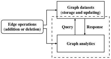
Figure 1: A framework of graph analytics in a dynamic system.

Figure 1 shows the outline of our framework for performing graph analytics in a dynamic system. Each time a new edge operation happens, the system maintains the graph dataset by adding or deleting the edge according to the operation, and updates the corresponding information which is determined by the service provided. This comprises the normal functioning of a dynamic graph-based system regardless of whether graph analytics is taken into consideration or not. Note that graph datasets have to be stored somewhere, typically on a server, and can be queried for graph analytics. In almost all real contexts, after all, we would not be counting the triangles in a graph without the graph existing in storage somewhere. Our framework, by assuming the existence of a stored graph dataset and allowing queries on it, achieves a better approximation of the reality of graph-based applications and networks.

For graph analytics, each new edge operation represents the addition or the deletion of an edge. There are streaming edge algorithms for various analytical purposes. Real-time algorithms for graph analytics will typically allow only a single pass over the edge stream. Based on the design of the algorithm, certain queries can be made of the server asking for additional information when processing a new edge. The availability of this additional information, via queries, is not an additional burden on the server since this information is often already updated and maintained by the service providers for offering necessary services.

In our framework for graph analytics, we assume the ability to process an edge stream (one pass) and also the ability to query the graph dataset server for information on the neighborhood of an edge. The dotted line in the figure frames the real-time graph analytics in a realistic scenario. In this framework, each new edge operation is treated as an arriving edge involving either an addition of an edge or the deletion of an edge. Edges are sampled independently with a certain probability. If an edge is sampled, queries are sent to the server asking for the information on the neighborhood of the two incident nodes of the sampled edge in order to update the estimators used in graph analytics.

We use the above framework to design a new sampling algorithm to keep a running count of the number of triangles in a dynamic graph. The estimation is enabled by the use of neighborhood information. Since the list of neighbors of a user is necessary information for a social network’s server to maintain and update anyway, little extra computational/memory costs are expended for querying this additional information.

1.2 Contributions

Based on the new framework/model of a dynamic graph system, we propose a new edge sampling algorithm, called Edge Sample and Discard (esd), which returns an estimate of the total number of triangles in a large dynamic graph by sampling only a tiny fraction of the edges in the graph. For each sampled edge, it samples the presence of triangles at the end points of the edge to update its estimates and then discards the edge (as opposed to holding the edge in memory in a subgraph sample as in [1, 30, 15]). The algorithm works on fully dynamic graphs where both edge deletions and additions are considered, and can be readily applied to static graphs as well. A preliminary version of this work appeared in [12].

In Section 2, we introduce the graph model more formally and present the esd algorithm. We show that the total number of triangles can be estimated from the probabilities with which we sample an edge and one of its neighbor nodes, and whether the sampled edge and the node form a triangle.

Section 3 presents a theoretical analysis of the algorithm and proves that its estimate is an unbiased one. We also derive a bound on the variance of our estimate and draw implications from it. We show that our sampling algorithm for an evolving graph can be readily modified to apply to static graphs.

Section 4 provides a comparative analysis of esd against two edge sampling algorithms, doulion [30] and trièst [26] which also can handle both edge additions and deletions, and provide a real-time tracking of the number of triangles. Note that the framework assumed by both doulion and trièst are slightly different from the one assumed by our algorithm. They are designed assuming traditional streaming edge framework and do not consider the possibility of using additional information obtained by querying the stored graph dataset on the server. We use several real network graphs with millions of edges to create streams of dynamic graphs. Based on tests on these graphs, we show that, with the use of the neighborhood information of the sampled edges, the accuracy achieved by esd is at least one order of magnitude better than the accuracies achieved by doulion and trièst, while the extra cost of querying for additional information is relatively small. These costs and the associated trade-offs are described in Section 4.

Section 4 also evaluates our algorithm on real dynamic graphs. The tests show that our algorithm can generate accurate estimates of the number of triangles in real dynamic graphs. Moreover, we present the influence of the total number of triangles and the clustering coefficient on the accuracy of the estimate of esd by performing simulations on Barab$\mathrm{\acute{a}}$si-Albert (BA) graphs. The accuracy achieved by our algorithm is better on graphs with a larger number of triangles or a larger global clustering coefficient.

Section 5 concludes the paper.

1.3 Related Work

Triadic properties such as triangle counts and the global clustering coefficient have been widely studied [7, 32]. Some early works use enumeration or matrix multiplication to compute the exact number of triangles in the graph [24, 18, 9, 8]. Alon et al. [2] propose the theoretically fastest exact triangle counting algorithm, which is based on fast matrix multiplication and runs in $O(|E|^{1.41})$ time. But it has a high space complexity of $O(|V|^{2})$ which renders it largely infeasible for extremely large graphs. Besides, in many cases, the exact answer is not necessary and an approximation is sufficient. Therefore, well-performing approximation methods, which achieve fast runtime and small memory footprint, have attracted tremendous interest.

Eigenvalue-based methods are one class of algorithms used to approximate the global and local number of triangles in the graph [3, 29]. They use the interesting property that the total number of triangles in an undirected graph is $1/6$ of the sum of the cubes of the eigenvalues of its adjacency matrix. But the computation of matrix multiplication is still very expensive and they only work on static graphs. Hardiman et al. [13] presents a method based on a random walk which is capable of estimating both the global and the average clustering coefficient by testing the connectivity of each node in the random walk after the mixing time is reached.

Most of the studies on triangle counting use the graph stream model, where a graph is treated as a stream of edges. Two algorithms for approximating the local number of triangles in both directed and undirected graph are presented in [4]. These two algorithms both require multiple passes over the edge stream and only work on static graphs.

Another class of algorithms uses an edge sparsification approach based on a certain selecting probability to decide whether an edge should be sampled [1, 30, 20]. In [16], a hybrid approach is used which combines edge sparsification with degree-based vertex partitioning. In all of these algorithms, the sample size is not fixed. Algorithms bases on reservoir sampling, which use a fixed amount of space for estimating the triadic properties, are described in [15, 25]. However, except for the method presented in [30], none of these algorithms can handle edge deletions in an evolving graph; they work on static graphs and on dynamic graphs with edge additions but not edge deletions.

One approach which works on fully dynamic graphs where both edge additions and deletions are allowed is presented in [17]. It combines the sampling of vertex triples algorithm in [6] and monochromatic sampling method in [22]. The algorithm first performs monochromatic sampling on the original large graph to obtain a sampled graph, and then estimates the global clustering coefficient by checking the closure of wedges selected in the sampled graph. The estimate of the total number of wedges in the original graph is obtained by applying the second moment estimation method in [27]. This algorithm has a large memory requirement and cannot provide a real-time update of the estimates. De Stefani et al. [26] propose a method based on reservoir sampling called trièst, which also works on fully dynamic graphs. It adopts random pairing [11], an extension of the reservoir sampling, to solve the problem of accounting for edge deletions. This algorithm uses a fixed sample size and can keep updating the estimates during the processing of the graph. Since the publication of our preliminary work in [12], a similar approach has been used in a recently published report [31]. However, they limit their focus on estimating the number of triangles on static graphs, and do not consider the dynamic case.

As presented in [26], trièst is significantly better than previously known methods in terms of accuracy, space requirement and the applicability to fully dynamic graphs. Even though the graph dataset in most real applications has to be stored somewhere, such as on a server accessible by API queries, the framework assumed by trièst does not permit queries to the graph dataset. The Edge Sample and Discard (esd), proposed in this paper, assumes a slightly different but more realistic framework allowing access to the graph dataset information to help substantially improve both the computational/memory costs and the accuracy.

2 The Algorithm

The Edge Sample and Discard (esd) algorithm is designed assuming the framework described in Section 1.1. It works on dynamic graphs where both edge deletions and additions are considered. Additional information, the neighboring nodes of the sampled edges, is queried. It is also generalizable to the case of directed graphs, but for clarity of presentation in the paper, we will use undirected graphs in this paper.

2.1 Preliminaries and Notation

Let $G_{t}=(V_{t},E_{t})$ represent an undirected simple graph, where $t$ is the time instant and $t\geq 0$. $V_{t}$ and $E_{t}$ are the node set and the edge set at time $t$, respectively. At the beginning, we have $V_{0}=E_{0}=\emptyset$.

Consider a stream $\mathcal{S}$ of $((u,v),\beta)$, where $(u,v)$ denotes the edge which is added to or deleted from the graph, and $\beta\in\{+1,-1\}$. $\beta=+1$ indicates that edge $(u,v)$ is added to the graph, and $\beta=-1$ indicates that edge $(u,v)$ is deleted from the graph. For any $t\geq 0$, if a new pair $((u,v),\beta)$ arrives at time $t$, we update $G_{t-1}=(V_{t-1},E_{t-1})$ to $G_{t}=(V_{t},E_{t})$ with the corresponding edge addition or deletion.

For simplicity, we drop $t$ from the notation and denote by $G=(V,E)$ the most recent update of the graph. Let $\Gamma(v)$ denote the set of neighbors of node $v\in V$, and let $d(v)=|\Gamma(v)|$ denote the node-degree of $v$. A wedge is a path of length two, and a triangle is a closed wedge (a circular path of length three). Let $T$ denote the set of triangles in $G$ and let $N_{T}=|T|$.

The goal of this work is to monitor the edge stream of a graph and estimate the value of $N_{T}$ by examining only a small fraction of the edges and their neighborhoods.

2.2 Edge Sample and Discard

Algorithm 1 presents the pseudo-code of Edge Sample and Discard (esd) to estimate the total number of triangles given a stream of $((u,v),\beta)$. In our algorithm, we use a global variable $T_{\mathrm{est}}$ to record the real-time estimate of the total number of triangles in the current graph. We consider both edge addition and deletion operations are included; however, as described in Figure 1 and as in real-life scenarios, the SNS server assumes responsibility for the maintenance and update of the graph datasets while the information related to the dataset can be queried and obtained by esd.

Lines 1-2 in the pseudo-code perform necessary initializations. Lines 3-8 show that for each pair $((u,v),\beta)$ in the stream, we check the value of $\beta$ and decide whether edge addition or deletion should be performed. Lines 9-13 perform edge sampling and estimate. We use the sampling fraction $\alpha$ as the selecting probability. Each arriving edge has a probability $\alpha$ of being sampled. If an edge is sampled, the UpdateCount routine is called. Note that UpdateCount works on the graph where the addition or deletion has just been made. Suppose, at time $t$, an edge $e=(u,v)$ is sampled and UpdateCount$(u,v,\beta)$ is called. Then, we examine the size of the neighborhood of $u$. For $\beta=-1$, when $(u,v)$ is deleted from $G_{t-1}$, we check whether node $u$ has neighbors in $G_{t}$. For $\beta=+1$, where $(u,v)$ is added to $G_{t-1}$, we check whether node $u$ has more than one neighbor in $G_{t}$. If one of the requirements is fulfilled, we check the value of $\beta$ and perform the corresponding neighborhood selection. If $\beta=+1$, we pick one node from the neighbor set of $u$ other than $v$. For example, we select node $a$ from $\Gamma(u)\setminus\{v\}$, and thus the probability of $a$ being picked uniformly at random is $\frac{1}{d(u)-1}$. Since the probability of sampling edge $(u,v)$ is $\alpha$, the total probability $P$ of selecting $(u,v)$ and then $a$ as a neighbor of $u$ is:

$$P=\frac{\alpha}{d(u)-1}.$$ (1)

Algorithm 1 The esd algorithm

1:A graph stream $\mathcal{S}$ and sampling fraction $\alpha$

2:$T_{\mathrm{est}}\leftarrow 0$

3:Create an empty graph $G$

4:for each pair $((u,v),\beta)$ in $\mathcal{S}$ do

5:     if $\beta=+1$ then

6:         Add new edge $(u,v)$ to graph $G$

7:     else

8:         Delete old edge $(u,v)$ from graph $G$

9:     end if

10:     $r\leftarrow$ Random number $\in[0,1]$

11:     if $r\leq\alpha$ then

12:         UpdateCount$(u,v,\beta)$

13:         UpdateCount$(v,u,\beta)$

14:     end if

15:end for

16:return $T_{\mathrm{est}}$

 

1:Function used in the esd algorithm  

2:UpdateCount$(u,v,\beta)$:

3:if $|\Gamma(u)|>\frac{1+\beta}{2}$ then

4:     if $\beta=+1$ then

5:         Pick random node $a$ uniformly from $\Gamma(u)\setminus\{v\}$

6:         if $a\in\Gamma(v)$ then

7:              $T_{\mathrm{est}}=T_{\mathrm{est}}+\frac{1}{2}\frac{d(u)-1}{\alpha}$

8:         end if

9:     else

10:         Pick random node $a$ uniformly from $\Gamma(u)$

11:         if $a\in\Gamma(v)$ then

12:              $T_{\mathrm{est}}=T_{\mathrm{est}}-\frac{1}{2}\frac{d(u)}{\alpha}$

13:         end if

14:     end if

15:end if

Given a wedge $a$-$u$-$v$, we check whether the closing edge $(a,v)$ exists by examining $\Gamma(v)$. If $a\in\Gamma(v)$, we update the triangle estimator $T_{\mathrm{est}}$. The estimate is updated by applying Eq. (5) (in Section 3). On the other hand, if $\beta=-1$, since edge $(u,v)$ is already deleted from $G$ and $v$ is no longer a neighbor of $u$, we pick one node from the neighbor set of $u$. Thus, the total probability $P$ of selecting $(u,v)$ and then one node from the neighborhood of $u$ is

$$P=\frac{\alpha}{d(u)}.$$ (2)

After selecting a node from the neighbor set of $u$, we check whether the selected node is also a neighbor of $v$. If it is, which means the subgraph induced by the two incident nodes of the deleted edge $(u,v)$ and the selected node together is a triangle in $G_{t-1}$, we update the triangle estimator $T_{\mathrm{est}}$.

Given a dynamic graph, esd avoids using extra space for storing the sample graph by discarding the processed edge and nodes after updating the estimate. The total number of triangles is estimated from the probabilities with which an edge and one of its neighbor nodes are sampled, and whether the sampled edge and the node form a triangle. esd can provide a real-time estimate of the triangle counts in a dynamic graph as new edges come in or old edges are deleted.

3 Quality of Estimation

In this section, we present the mathematical reasoning behind our triangle estimator and prove that our algorithm provides an unbiased estimate of the total number of triangles with a theoretically tight bound on the variance. We first discuss the case of dynamic graphs allowing only the addition of edges and with edge deletions not considered; we next show that estimating the number of triangles in this additions-only case is not different from that in the case of a fully dynamic graph with both additions and deletions.

Let an ordered tuple $(u,v,z)$ denote the sampled edge $(u,v)$ and the node $z$ selected by UpdateCount$(u,v,\beta)$. The first element in the tuple, $u$, is one of the incident nodes of the edge and the second element is the other incident node. The third element of the tuple, $z$, is the node picked from the neighborhood of the first element, $u$. For example, given a sampled pair $((a,b),+1)$ from the edge stream, we select node $c$ from $\Gamma(a)\setminus\{b\}$ which gives us the ordered tuple $(a,b,c)$.

Let’s consider the partially dynamic case with edge additions only. Suppose we have a stream $\mathcal{S}$ of pairs $((u,v),\beta)$ where $\beta=+1$ for each pair in $\mathcal{S}$. If a pair $((u,v),+1)$ arrives at time $t$, the graph $G_{t-1}$ is updated to $G_{t}$ as follows:

$$G_{t}=(V_{t-1}\cup\{u,v\},E_{t-1}\cup\{(u,v)\}).$$

Let $T_{t}$ denote the set of triangles in $G_{t}$, where $T_{0}=\emptyset$. Suppose, at time $t+1$, we get $(e_{t+1},+1)$ from the stream, where $e_{t+1}=(u,v)$ is an edge arriving at time $t+1$ , so we have an updated graph $G_{t+1}$. Let $H(e_{t},G_{t})$ denote the set of triangles composed of edge $e_{t}$ in graph $G_{t}$. We can obtain that $T_{t+1}=T_{t}\cup H(e_{t+1},G_{t+1})$. Since $T_{t}\cap H(e_{t+1},G_{t+1})=\emptyset$,

$$|T_{t+1}|=|T_{t}|+|H(e_{t+1},G_{t+1})|.$$ (3)

According to Eq. (3), we can obtain:

$$|T_{t}|=\sum_{i=0}^{t}{|H(e_{i},G_{i})|}.$$ (4)

Let $\mathcal{Q}_{t}$ denote the set of all ordered tuples $(u,v,z)$ that have a non-zero probability to be observed when processing a new arriving pair $(e_{t},\beta)$ from stream $\mathcal{S}$. Let $\mathcal{T}_{t}\subseteq\mathcal{Q}_{t}$ be the set of all ordered tuples in $\mathcal{Q}_{t}$ of which the three elements form a triangle in $G_{t}$. Note that $(u,v,z)$ and $(v,u,z)$ are two different tuples but the three elements in each of them induce the same triangle in the graph.

Suppose $(e_{t},\beta)$ is sampled, and then one node is picked from the neighborhood of each incident node of $e_{t}$. So the same triangle may be observed twice during the sampling period. Thus, we can obtain

$$|\mathcal{T}_{t}|=2|H(e_{t},G_{t})|.$$

Consider $\mathcal{T}_{t}^{\prime}\subseteq\mathcal{T}_{t}$ as the set of ordered tuples obtained by sampling $(e_{t},+1)$ , where the three elements of each ordered tuple in $\mathcal{T}_{t}^{\prime}$ form a triangle in $G_{t}$. Let $P(r)$ be the probability that an ordered tuple $r=(u,v,z)\in\mathcal{T}_{t}^{\prime}$ is sampled. By adopting the Horvitz-Thompson construction[14], we come up with the linear estimator,

$$H^{t}_{\mathrm{est}}=\omega\sum_{r\in\mathcal{T}_{t}^{\prime}}\frac{1}{P(r)}.$$ (5)

$\omega$ is a weight parameter, and $\omega=|H(e_{t},G_{t})|/|\mathcal{T}_{t}|=1/2$.

Let $\Delta_{k}=(u,v,z)$ be an element in $\mathcal{T}_{t}$, where $k\in[1,|\mathcal{T}_{t}|]$. Remember that the subgraph induced by the three elements of $\Delta_{k}$ in $G_{t}$ is a triangle. Let $\delta_{k}$ denote the existence of $\Delta_{k}$ in the set $\mathcal{T}_{t}^{\prime}$. We have

$$\delta_{k}=\left\{\begin{array}[]{ll}1&\mbox{ $\Delta_{k}\in\mathcal{T}_{t}^{\prime}$}\\ 0&\mbox{ $\Delta_{k}\notin\mathcal{T}_{t}^{\prime}$}\end{array}\right.$$

Taking the expectation of $H^{t}_{\mathrm{est}}$,

$$\mathrm{E}[H^{t}_{\mathrm{est}}] = \omega\sum_{k=1}^{|\mathcal{T}_{t}|}\mathrm{E}[\delta_{k}\cdot\frac{1}{P(\Delta_{k})}]$$

$$= \omega\sum_{k=1}^{|\mathcal{T}_{t}|}P(\Delta_{k})\cdot\frac{1}{P(\Delta_{k})}$$

$$= |H(e_{t},G_{t})|$$

The expected number of triangles composed of edge $e_{t}$ obtained by our estimator is equal to the actual number of triangles composed of edge $e_{t}$ in $G_{t}$. Applying Eq. (4) and Eq. (5), we get:

$$|T_{t}|_{\mathrm{est}}=\omega\sum_{i=0}^{t}\sum_{r\in\mathcal{T}_{t}^{\prime}}\frac{1}{P(r)}$$

According to the linearity of the expectation, $\mathrm{E}[|T_{t}|_{\mathrm{est}}]=|T_{t}|$. So we have an unbiased estimator to approximate the total number of triangles in $G_{t}$. The variance of $H^{t}_{\mathrm{est}}$ is:

$$\mathrm{Var}[H^{t}_{\mathrm{est}}] = \mathrm{E}[(H^{t}_{\mathrm{est}}-\mathrm{E}[H^{t}_{\mathrm{est}}])^{2}]$$

$$= \mathrm{E}[{H^{t}_{\mathrm{est}}}^{2}]-|H(e_{t},G_{t})|^{2}$$

Expanding $\mathrm{E}[{H^{t}_{\mathrm{est}}}^{2}]$, we get:

$$\mathrm{E}[{H^{t}_{\mathrm{est}}}^{2}] = \omega^{2}\,\mathrm{E}\left[\sum_{i=1}^{|\mathcal{T}_{t}|}\left(\frac{\delta_{i}}{P(\Delta_{i})}\right)^{2}+\sum_{i\neq j}^{|\mathcal{T}_{t}|}\frac{\delta_{i}\delta_{j}}{P(\Delta_{i})P(\Delta_{j})}\right]$$

Suppose the sampling fraction is $\alpha$, and the maximum degree in $G_{t}$ (the graph upon the most recent update) is $d_{\mathrm{max}}$, then we have $P(\Delta_{i})\geq\frac{\alpha}{d_{\mathrm{max}}-1}$ for any $i\in[1,|\mathcal{T}_{t}|]$. Letting $m=\frac{\alpha}{d_{\mathrm{max}}-1}$, we can obtain,

$$\mathrm{E}\left[\sum_{i=1}^{|\mathcal{T}_{t}|}\left(\frac{\delta_{i}}{P(\Delta_{i})}\right)^{2}\right]\leq|\mathcal{T}_{t}|\frac{1}{m}$$

According to the definition of $\mathcal{T}_{t}$, each ordered-tuple in $\mathcal{T}_{t}$ represents the triangle which is part of edge $e_{t}$ in $G_{t}$. So the two triangles represented by any two ordered-tuples $\Delta_{i}$ and $\Delta_{j}$ in set $\mathcal{T}_{t}$, where $i\neq j$, must have edge $e_{t}$ as a shared edge. Thus,

$$\mathrm{E}\left[\sum_{i\neq j}^{|\mathcal{T}_{t}|}\frac{\delta_{i}\delta_{j}}{P(\Delta_{i})P(\Delta_{j})}\right]=\frac{2}{\alpha}\left(\frac{|\mathcal{T}_{t}|}{2}\right)^{2}$$

So the variance of our estimator is bounded as follows,

$$\mathrm{Var}[H^{t}_{\mathrm{est}}]\leq\frac{|\mathcal{T}_{t}|(d_{\mathrm{max}}-1)}{4\alpha}+\left(\frac{1}{2\alpha}-1\right)\left(\frac{|\mathcal{T}_{t}|}{2}\right)^{2}$$

Since $\mathrm{Var}[|T_{t}|_{\mathrm{est}}]=\sum_{i=0}^{t}\mathrm{Var}[H^{t}_{\mathrm{est}}]$, we have

$$\mathrm{Var}[|T_{t}|_{\mathrm{est}}]\leq\frac{|T_{t}|(d_{\mathrm{max}}-1)}{2\alpha}+\sum_{i=0}^{t}|H(e_{t},G_{t})|^{2}\left(\frac{1}{2\alpha}-1\right)$$

For any $t>0$, when the degree of the incident nodes of the sampled edge in $G_{t}$, where $t$ is the time step that the edge is sampled, are all equal, the equality in the above bound holds. Therefore, the bound derived above on the variance of our estimate, $\mathrm{Var}[|T_{t}|_{\mathrm{est}}]$, is a strict upper bound.

Further, applying Chebyshev’s inequality

$$P(||T_{t}|_{\mathrm{est}}-|T_{t}||\geqslant\epsilon|T_{t}|)\leqslant\frac{\mathrm{Var}[|T_{t}|_{\mathrm{est}}]}{\epsilon^{2}|T_{t}|^{2}}$$ (6)

The above shows that the relative error of the estimate is influenced by the sampling fraction and the properties of the graph. The error is increased as the value of the sampling fraction is decreased and the estimate achieves a better accuracy on a graph with more triangles. Moreover, the local clustering coefficient also affects the estimate; the algorithm can achieve a better accuracy on a graph where most of the nodes have a higher clustering coefficient. In general, esd achieves a better estimate on graphs with a higher global clustering coefficient.

The proof for the fully dynamic case with edge deletions is similar to the case with additions described above. Suppose we keep performing edge addition up to time $t$. Thus, at time $t$, we have a graph $G_{t}=(V_{t},E_{t})$ and $T_{t}$, the set of triangles in $G_{t}$. Suppose, at time $t+1$, we get $(e_{t+1},-1)$ from the stream, indicating an edge deletion, so we have an updated graph $G_{t+1}$. We can easily obtain that $T_{t+1}=T_{t}\setminus H(e_{t+1},G_{t})$. In other words, we have

$$|T_{t+1}|=|T_{t}|-|H(e_{t+1},G_{t})|.$$

As proved before, we have an unbiased estimator $H^{t}_{\mathrm{est}}$ for estimating $|H(e_{t},G_{t})|$, so in the edge deletion case, we use the same estimator to estimate the decreased number of triangles caused by deleting $e_{t+1}$.

3.1 Static graphs

Although esd is designed for implementation on dynamic graphs, it can be easily extended to work on static graphs. In the dynamic case, a triangle can be detected only when the new coming edge is the closing edge of a wedge already in the graph; however, in static graphs, each of the three edges of a triangle appears in the edge stream, so one triangle can be detected every time the new coming edge is part of this triangle. Thus, for static graphs, the value of the weight parameter $\omega$ of the estimator is one-third of the one in the dynamic case.

Let $\mathcal{S}^{\prime}$ be the set of ordered tuples which represent the triangles observed in the sampling period by an edge stream which delivers random edges from the static graph. Let $P(s)$ be the probability that a tuple $s\in\mathcal{S}^{\prime}$ is sampled. By applying the Horvitz-Thompson construction, we have:

$$|T|_{\mathrm{est}}=\omega\sum_{s\in\mathcal{S}^{\prime}}\frac{1}{P(s)}$$

where the weight parameter is $\omega=1/6$.

4 Performance Analysis

In this section, we perform a comparative analysis of the performance of esd against trièst [26] and doulion[30]. Both trièst and doulion, like esd, can provide a real-time estimate of the total number of triangles by performing edge sampling on an edge stream of a fully dynamic graph. However, trièst and doulion assume a traditional streaming graph framework, where a graph can be processed only via a stream of edges. As our comparative analysis will show, the use of additional information by esd already available and kept updated for graph maintenance as per our framework, substantially improves the accuracy.

We use real, simple and undirected graphs from the Network Repository site [23] to create streams of addition-only graphs and fully dynamic graphs. Table 1 summarizes some vital properties of these graphs. We also evaluate our algorithm on two real dynamic graphs from [19] and [34].

Table 1: Properties of the graphs used in the experiments. $|E|$ is the number of edges, $|V|$ is the number of nodes, $N_{T}$ is the number of triangles and $\eta$ is the global clustering coefficient.

Graph	$|E|$	$|V|$	$N_{T}$	$\eta$
socfb-UCLA	7.47e+05	2.05e+04	5.11e+06	0.1431
socfb-Wisconsin	8.35e+05	2.38e+04	4.86e+06	0.1201
com-Amazon	9.26e+05	5.49e+05	6.67e+05	0.2052
com-DBLP	1.05e+06	4.26e+05	2.22e+06	0.3064
web-Stanford	1.99e+06	2.82e+05	1.13e+07	0.0086
web-Google	4.32e+06	8.76e+05	1.34e+07	0.0552

4.1 Complexity

Table 2: The complexity of the three algorithms.

Algorithm	Time complexity	Server-side time complexity	Space complexity	Server-side space complexity
esd	$O(p|E|\log d_{G})$	$O(p|E|)$	$O(d_{G})$	$O(d_{G})$
doulion1	$O(p|E|+(p|E|)^{\frac{2\omega}{\omega+1}})$	N/A	$O({V_{s}}^{2})$	N/A
trièst	$O(Md_{s}\log|E|\log d_{s})$	N/A	$O(M)$	N/A

• The algorithm given in [30] cannot provide a real-time estimate; it only updates the estimate once after processing the entire graph.

Fast runtime and small space requirement are two vital goals of a good sampling algorithm.

4.1.1 Runtime

Consider the partially dynamic case where edge additions happen $|E|$ times and there are no edge deletions. Suppose the neighbors of each node in a graph are stored in a sorted list. This allows a determination of whether a node is a neighbor of another specific node in $O(\log d)$ steps where $d$ is the degree of that specific node.

In trièst, an edge reservoir is maintained and updated. Suppose the size of the edge reservoir is $M$. At time $t$ ($t>M$), the probability of updating the edge reservoir is $M/t$, so the expected number of times that the edge reservoir is updated is $M+\sum_{t=M+1}^{|E|}\frac{M}{t}\approx M+M\ln|E|.$ Each time the edge reservoir is updated, trièst checks the number of triangles composed of the newly sampled edge in the sample graph. Suppose $d_{s}$ is the maximum degree in the sample graph, the computational complexity of trièst is $O(Md_{s}\log|E|\log d_{s})$.

As presented in [30], the computational complexity of doulion is $O(p|E|+(p|E|)^{\frac{2\omega}{\omega+1}})$, where $\omega$ is 2.371 and $p$ is the probability of sampling an edge.

In the case of ESD, suppose $p|E|$ is the number of edges which are sampled, and each query of the neighbor nodes takes O(1). Then, for each sampled edge, we take a maximum of $O(\log d_{G})$ steps to sample a neighboring node and determine if the node and the sampled edge form a triangle. The complexity of esd, therefore, is $O(p|E|\log d_{G})$. Besides, the server needs to take $O(p|E|)$ to respond to the queries.

Table 2 summaries the complexity of the three algorithms for the case with no edge deletions. esd is faster than doulion when $\log d_{G}<(p|E|)^{0.41}$ (the number of edges sampled is not too small). In fact, on all real graphs today and reasonable sample sizes, esd enjoys a lower computational complexity than doulion. For esd and trièst, since $\log|E|>\log d_{G}$ for large graphs, esd is faster then trièst when sampling the same number of edges ($p|E|=M$).

Moreover, for each edge deletion, both doulion and trièst have to check whether the deleted edge is in the sample set or not, and update the estimates. While in esd, it avoids looking up the sample set and processes edge deletions with a sampling probability. So our algorithm is substantially faster than doulion and trièst, especially when facing a large amount of edge deletions.

Note that esd uses a different framework from doulion and trièst, neither of which involve querying the server for additional information. Given the framework used by esd, it involves an additional server-side cost in responding to the queries. As shown in Table 2, esd achieves a substantially better trade-off saving computational and memory costs with a small amount of extra effort on the part of the server.

4.1.2 Space

At first sight, it may appear as though the framework used in this paper to develop the ESD algorithm requires the storage of the entire graph while doulion and trièst only have to store the sampled graph. However, this mischaracterizes the actual storage needs under these frameworks. In real contexts, even streaming graph data for a fully dynamic graph are ultimately generated by a system/server which maintains and keeps updated a graph dataset. After all, a well-maintained graph dataset is essential for the normal functioning of most applications relying on the graph. Before, after and in the midst of any graph analytics, in most real contexts, the graph datasets are still kept stored somewhere. So even for the traditional streaming graph model (used by trièst and doulion), the existence and the storage needs of the complete graph dataset cannot and should not be ignored. It is unrealistic to assume that, after performing a streaming graph algorithm, one would only store the sampled graph and not store anywhere the large dynamic graph observed so far. Therefore, the cost of storing the dynamic graph is a necessity for all of the three algorithms and their respective frameworks.

For the graph analytics part, our algorithm avoids the requirement of extra memory to store the sampled edges by performing independent collections of edges and discarding edges after updating the estimators. The list of the neighbor nodes of the sampled edge are required for estimating which leads to a memory requirement $O(d_{G})$ where $d_{G}$ is the maximum degree in the original graph. As described in Section 1.1, the graph datasets are maintained regardless of whether the graph analytics is applied or not. Thus, for the server-side space complexity, we do not include the cost for maintaining the graph datasets, and only count the extra space complexity required by our algorithm.

doulion uses a certain probability $p$ to sample edges in the stream, and the samples are maintained in the memory during the entire process. So the amount of memory used is not fixed and partially depends on the algorithm used to calculate the exact number of triangles in the sampled graph. In [30], the fast matrix multiplication is used to count triangles in the sampled graph, so the space complexity is $O({V_{s}}^{2})$, where $V_{s}$ is the number of nodes in the sampled graph. trièst is a reservoir sampling based algorithm which uses a fixed amount of memory to store the sampled edges.

4.2 Partially dynamic case

We show the comparison of the performances of esd with trièst and doulion on dynamic graphs where only edge additions are considered. The edge stream is generated by permuting the edges uniformly at random.

We consider the relative error in estimating the triangle number as a measure of the accuracy. The relative error is measured as:

$$\mathrm{Relative~{}error}=\frac{\mathrm{Average~{}estimate}-\mathrm{Actual~{}value}}{\mathrm{Actual~{}value}},$$

where the average estimate is the mean of the estimated value over 100 independent runs.

Table 3: The relative errors in the estimates of the total number of triangles. Sample size is the number of edges sampled.

		Triangles $N_{T}$
Graph	Sample	Relative error (%)
name	size	esd	doulion	trièst
socfb-UCLA	7,476	0.0958	1.6274	3.5433
socfb-Wisconsin	8,359	0.5380	4.2736	2.6817
com-Amazon	9,258	0.2329	6.4262	3.4856
com-DBLP	10,498	0.4301	1.5458	3.4481
web-Stanford	19,926	0.9796	3.1822	5.6751
web-Google	43,220	0.0336	2.2997	3.2821

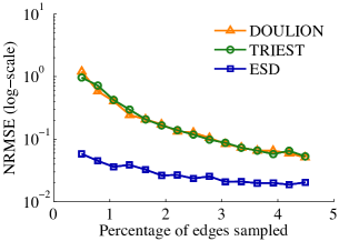
(a) socfb-UCLA

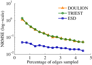
(b) socfb-Wisconsin

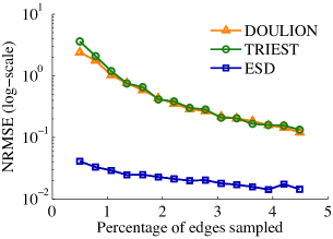
(c) com-Amazon

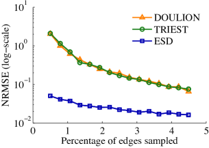
(d) com-DBLP

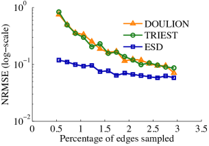
(e) web-Stanford

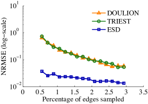
(f) web-Google

Figure 2: Comparison of NRMSEs of the estimates for three algorithms over 100 independent runs.

Table 3 shows relative errors in estimating the total number of triangles for each of the three algorithms. We sample 1% of the edges for each graph. As shown in the table, esd achieves better accuracy than the other algorithms on all the graphs. On most of the graphs, the relative errors obtained by esd are at least one order of magnitude smaller than the errors obtained by doulion and trièst.

To further compare the accuracy of the three algorithms, we use the normalized root mean square error:

$$\mathrm{NRMSE}=\frac{\sqrt{\mathrm{E}[(\mathrm{estimate}-\mathrm{Actual~{}value})^{2}]}}{\mathrm{Actual~{}value}},$$

Figure 2 depicts the average NRMSEs based on 100 independent runs for each graph as the sample sizes are increased. We can see from the figure that esd has the smallest NRMSEs in all cases. Especially when the sample size is small, the NRMSEs of esd are almost one order of magnitude smaller than the NRMSEs of doulion and trièst. On most of the graphs, our algorithm achieves similar NRMSEs to the other two algorithms with one-ninth of the sample size used by these two algorithms. In other words, to achieve equivalent accuracy, esd requires fewer samples, and thus reduces the computational cost.

4.3 Fully dynamic graphs

In the experiments for the fully dynamic case, we use the model presented in [26] to simulate the deletions or additions of nodes or edges.

We first tested the performances of the three algorithms on dynamic graphs where both edge additions and deletions are considered. For each test on the graph, we first generate a stream of edges by randomly permuting the edges. Initially, an empty graph $G$ is created. The arrival of each edge in the stream is treated as an edge addition, and each new edge is added into $G$. A probability $p_{e}=0.0001$ is used to decide whether a deletion event should be performed after each edge addition is made. If a deletion event happens, every edge in $G$ has a probability $p_{d}=0.01$ of being deleted.

(a) socfb-UCLA

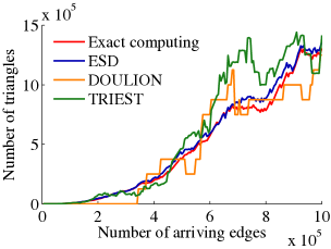
(b) socfb-Wisconsin87

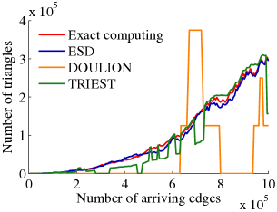
(c) com-DBLP

Figure 3: Comparison of the estimated values of total number of triangles in dynamic case.

Figure 3 shows the comparison of the estimates of the triangle number for three algorithms. The red line indicates the actual number of triangles obtained by the exact triangle computing algorithm. For all graphs, the final sample sizes of both doulion and esd are approximately equal to 10,000, while the sample size of trièst is fixed at 10,000.

As shown in the figure, esd has the best performance among the three in tracking the changes in the number of triangles, even at small sample sizes. In the case of doulion, however, the edge deletion affects the accuracy of its estimate. If many deleted edges are edges held in the sample set, the sample set shrinks quickly, significantly reducing the accuracy of estimates made by doulion. For example, in the com-DBLP graph, the estimate obtained by doulion is sometimes more than twice as large as the actual value.

trièst uses reservoir sampling with a fixed size of the sample set. If the deleted edge is an edge in the sample set, it would be removed from the sample set, and the edge deletion in the sample set would be compensated by future edge insertion. So trièst can maintain a sample set with fixed number of edges during the entire sampling period. In other words, the number of edges sampled by trièst is always larger than the number of edges sampled by esd and doulion in the simulations. The figure shows that esd achieves a better performance than trièst in terms of the accuracy even though trièst samples more edges than esd.

Besides edge deletion, in the real world, node deletion also occurs. Deletion of a single node can be modeled as a sequence of deletions of edges adjacent to that node. We also tested the performances of the three algorithms on dynamic graphs with node deletions. For each test on the graph, we use a probability $p_{e}=0.0001$ to decide whether a deletion event should be performed after the occurrence of each edge addition. If a deletion event happens, every node in the current graph has a probability $p_{d}=0.001$ of being deleted.

Figure 4 plots the comparison of the estimates of the number of triangles for the three algorithms. For all graphs, the sampling probability is set to 0.02 for doulion and is set to 0.01 for esd, while the sample size of trièst is fixed at 10,000.

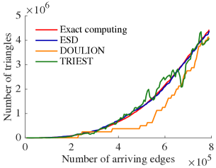
(a) socfb-UCLA

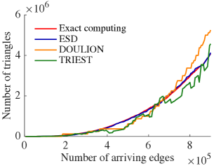
(b) socfb-Wisconsin87

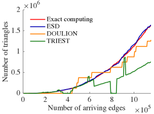
(c) com-DBLP

Figure 4: Comparison of the estimated values of total number of triangles in dynamic case.

As plotted in the figure, esd achieves the best performance among the three in estimating the number of triangles in dynamic graphs with node deletions. The red line which indicates the actual number of triangles, is extremely close to the blue line which plots the estimates obtained by esd. The closeness between the red line and the blue line indicates that our algorithm is capable of providing accurate estimates of number of triangles in a real-time fashion. Moreover, for all graphs, esd has the smallest final sample size. In other words, our algorithm samples fewer edges, but achieves higher accuracy than the other two algorithms in tracking the number of triangles.

Besides the above mentioned models, we also tested the performance of our algorithm on two real dynamic graphs. Oregon-2 dataset [19] contains 9 autonomous system (AS) graphs which represent AS peering information inferred from Oregon route-views. It was collected from March 31, 2001, to May 26, 2001. Yahoo! Message dataset [34] which has 28 graphs, was generated by a small subset of Yahoo! Messenger users from different zip codes for 28 days starting from April 1, 2008. Graphs in each of the datasets are timestamped. Each of the graphs is processed sequentially according to its time order. Edges which are not present in the previous graph, but are in the current graph, are treated as edge additions, and edges which are present in the previous graph, but are not in the current graph, are treated as edge deletions. Thus, both of the two datasets exhibit the addition and deletion of the edges over time.

Figure 5 shows the estimation of the total number of triangles on real dynamic graphs when the sampling fraction is $\alpha=0.01$. As shown in the figure, esd has a good performance on real graphs in terms of the accuracy and the variance. Even on the Yahoo! Message graph, where the number of triangles changes frequently and dramatically, our algorithm is still capable of tracking variation on the number of triangles accurately.

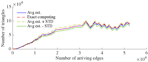
(a) Oregon-2

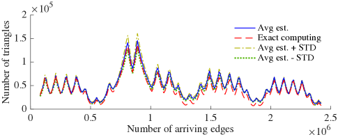
(b) Yahoo! Messenger

Figure 5: Estimation of the total number of triangles in dynamic case.

Table 4: Properties of the Barab$\mathrm{\acute{a}}$si-Albert (BA) graphs used in the experiments. $\gamma$ is the power of the preferential attachment, $N_{T}$ is the number of triangles, and $\eta$ is the global clustering coefficient.

Graph	$\gamma$	$N_{T}$	$\eta$	$|E|$	$|V|$
BA-1	1.5	281,296	0.00255	200,500	20,000
BA-2	1.5	1,046,132	0.00381	399,500	20,000
BA-3	1.5	6,874,145	0.01195	996,500	20,000
BA-4	1.0	3,526,361	0.02615	1,474,100	20,000
BA-5	1.5	3,473,097	0.00818	757,700	20,000
BA-6	2.0	3,464,420	0.00233	598,500	20,000

4.4 Relationship to graph properties

We show the influence of the properties of the graph on the performance of esd by testing on several Barab$\mathrm{\acute{a}}$si-Albert (BA) graphs. For ease in illustrating this relationship, we only consider edge-additions in this set of experiments. We ran esd on BA graphs with the same number of nodes, but with different numbers of edges and different powers of the preferential attachment. For each BA graph, we start with an Erd$\mathrm{\ddot{o}}$s-R$\mathrm{\acute{e}}$nzi graph with 100 nodes. Then, in each time step, one node is added to the graph, and the new node initiates dozens of edges to old nodes. The probability that an old node is selected is given by:

$$P(i)\thicksim{d_{i}}^{\gamma}$$

where $d_{i}$ is the degree of node $i$ in the current time step and $\gamma$ is the power of the preferential attachment. Table 4 lists some basic properties of the BA graphs used in these simulation experiments.

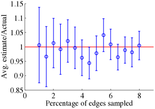
(a) BA-1 ($\gamma=1.5$, $N_{T}=281,296$)

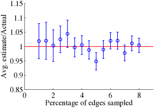
(b) BA-2 ($\gamma=1.5$, $N_{T}=1,046,132$)

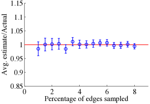
(c) BA-3 ($\gamma=1.5$, $N_{T}=6,874,145$)

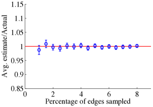
(d) BA-4 ($\gamma=1.0$, $N_{T}=3,526,361$)

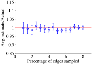
(e) BA-5 ($\gamma=1.5$, $N_{T}=3,473,097$)

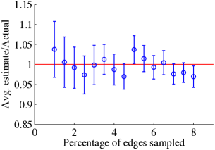
(f) BA-6 ($\gamma=2.0$, $N_{T}=3,464,420$)

Figure 6: Blue circles represent the ratio of the average estimated values of the total number of triangles to the actual value over 100 independent runs. Red line indicates 1. The blue error bars indicate 95% confidence intervals.

Figure 6 shows the ratio of the average estimated total number of triangles to the actual value for each BA graph with increasing number of edges sampled. The error bars represent the 95% confidence intervals. The red line indicates 1, when the estimated and the actual values are equal. For all of the graphs, the same sampling fraction is used. By comparing Figures 6$(a)$, 6$(b)$ and 6$(c)$ where all of these figures are obtained by testing on BA graphs with the same power of the preferential attachment, we can see that the confidence intervals are larger in the BA graphs with a smaller number of triangles. In Figures 6$(d)$, 6$(e)$ and 6(f), the total number of triangles in each of the tested graphs is approximately equal but the values of $\gamma$ and the global clustering coefficient are different. We can see that the estimate on graphs with a higher global clustering coefficient achieves a smaller confidence interval.

These results confirm the theoretical analysis of the relative error of the estimate presented in Section 3. Besides the sampling fraction, the relative error of the estimate is influenced by certain properties of the graph. Our algorithm achieves better accuracy on graphs with more triangles and a higher global clustering coefficient.

5 Conclusion

In this paper, we propose a new framework for analyzing graphs in a dynamic system, and present an edge sampling algorithm, called Edge Sample and Discard (esd), which estimates the total number of triangles in a fully dynamic graph where both edge additions and deletions are possible. With a tiny modification of the weight parameter, esd can also be applied to static graphs. Our algorithm achieves a significant improvement in accuracy by allowing the use of neighborhood information of the sampled edges through sending queries to the graph dataset. As illustrated in our performance analysis, esd achieves much better accuracy, smaller variance, and faster speed than the previously known state-of-the-art algorithms. In particular, it offers a methodology to keep track of the changes in the number of motifs of a certain type in a fully dynamic graph.

References

- [1] Ahmed, N.K., Duffield, N., Neville, J., Kompella, R.: Graph sample and hold: A framework for big-graph analytics. In: ACM KDD. pp. 1446–1455 (2014)
- [2] Alon, N., Yuster, R., Zwick, U.: Finding and counting given length cycles. Algorithmica 17(3), 209–223 (1997)
- [3] Avron, H.: Counting triangles in large graphs using randomized matrix trace estimation. In: Workshop on Large-scale Data Mining: Theory and Applications. vol. 10, pp. 10–9 (2010)
- [4] Becchetti, L., Boldi, P., Castillo, C., Gionis, A.: Efficient algorithms for large-scale local triangle counting. ACM TKDD 4(3), 13 (2010)
- [5] Berry, J.W., Hendrickson, B., LaViolette, R.A., Phillips, C.A.: Tolerating the community detection resolution limit with edge weighting. Physical Review E 83(5), 056119 (2011)
- [6] Buriol, L.S., Frahling, G., Leonardi, S., Marchetti-Spaccamela, A., Sohler, C.: Counting triangles in data streams. In: ACM SIGMOD-SIGACT-SIGART Symposium on Principles of Database Systems. pp. 253–262 (2006)
- [7] Chakrabarti, D., Faloutsos, C.: Graph mining: Laws, generators, and algorithms. ACM Computing Surveys (CSUR) 38(1), 2 (2006)
- [8] Chiba, N., Nishizeki, T.: Arboricity and subgraph listing algorithms. SIAM Journal on Computing 14(1), 210–223 (1985)
- [9] Coppersmith, D., Winograd, S.: Matrix multiplication via arithmetic progressions. In: Proceedings of the 19th annual ACM symposium on Theory of computing. pp. 1–6. ACM (1987)
- [10] Foucault Welles, B., Van Devender, A., Contractor, N.: Is a friend a friend?: Investigating the structure of friendship networks in virtual worlds. In: CHI’10 Extended Abstracts on Human Factors in Computing Systems. pp. 4027–4032. ACM (2010)
- [11] Gemulla, R., Lehner, W., Haas, P.J.: Maintaining bounded-size sample synopses of evolving datasets. The VLDB Journal-—The International Journal on Very Large Data Bases 17(2), 173–201 (2008)
- [12] Han, G., Sethu, H.: Edge sample and discard: A new algorithm for counting triangles in large dynamic graphs. In: IEEE/ACM International Conference on Advances in Social Networks Analysis and Mining. pp. 44–49. ACM (2017)
- [13] Hardiman, S.J., Katzir, L.: Estimating clustering coefficients and size of social networks via random walk. In: WWW. pp. 539–550 (2013)
- [14] Horvitz, D.G., Thompson, D.J.: A generalization of sampling without replacement from a finite universe. Journal of the American statistical Association 47(260), 663–685 (1952)
- [15] Jha, M., Seshadhri, C., Pinar, A.: A space-efficient streaming algorithm for estimating transitivity and triangle counts using the birthday paradox. ACM TKDD 9(3), 15 (2015)
- [16] Kolountzakis, M.N., Miller, G.L., Peng, R., Tsourakakis, C.E.: Efficient triangle counting in large graphs via degree-based vertex partitioning. Internet Mathematics 8(1-2), 161–185 (2012)
- [17] Kutzkov, K., Pagh, R.: Triangle counting in dynamic graph streams. In: Algorithm Theory–SWAT 2014, pp. 306–318. Springer (2014)
- [18] Latapy, M.: Main-memory triangle computations for very large (sparse (power-law)) graphs. Theoretical Computer Science 407(1), 458–473 (2008)
- [19] Leskovec, J., Krevl, A.: SNAP Datasets: Stanford large network dataset collection. http://snap.stanford.edu/data (Jun 2014)
- [20] Lim, Y., Kang, U.: Mascot: Memory-efficient and accurate sampling for counting local triangles in graph streams. In: ACM KDD. pp. 685–694. ACM (2015)
- [21] Newman, M.E.: The structure and function of complex networks. SIAM review 45(2), 167–256 (2003)
- [22] Pagh, R., Tsourakakis, C.E.: Colorful triangle counting and a mapreduce implementation. Information Processing Letters 112(7), 277–281 (2012)
- [23] Rossi, R.A., Ahmed, N.K.: The network data repository with interactive graph analytics and visualization (2013), http://networkrepository.com
- [24] Schank, T., Wagner, D.: Finding, counting and listing all triangles in large graphs, an experimental study. In: Experimental and Efficient Algorithms, pp. 606–609. Springer (2005)
- [25] Shin, K.: Wrs: Waiting room sampling for accurate triangle counting in real graph streams. arXiv preprint arXiv:1709.03147 (2017)
- [26] Stefani, L.D., Epasto, A., Riondato, M., Upfal, E.: TRIÈST: Counting local and global triangles in fully-dynamic streams with fixed memory size. CoRR abs/1602.07424 (2016), http://arxiv.org/abs/1602.07424
- [27] Thorup, M., Zhang, Y.: Tabulation-based 5-independent hashing with applications to linear probing and second moment estimation. SIAM Journal on Computing 41(2), 293–331 (2012)
- [28] Tiropanis, T., Hall, W., Crowcroft, J., Contractor, N., Tassiulas, L.: Network science, web science, and Internet science. Communications of the ACM 58(8), 76–82 (Jul 2015)
- [29] Tsourakakis, C.E.: Fast counting of triangles in large real networks without counting: Algorithms and laws. In: 2008 8th IEEE International Conference on Data Mining. pp. 608–617. IEEE (2008)
- [30] Tsourakakis, C.E., Kang, U., Miller, G.L., Faloutsos, C.: Doulion: Counting triangles in massive graphs with a coin. In: ACM KDD. pp. 837–846 (2009)
- [31] Türkoğlu, D., Turk, A.: Edge-based wedge sampling to estimate triangle counts in very large graphs. arXiv preprint arXiv:1710.09961 (2017)
- [32] Wasserman, S., Faust, K.: Social network analysis: Methods and applications, vol. 8. Cambridge University Press (1994)
- [33] Welser, H.T., Gleave, E., Fisher, D., Smith, M.: Visualizing the signatures of social roles in online discussion groups. Journal of Social Structure 8(2), 1–32 (2007)
- [34] Yahoo! webscope dataset. http://research.yahoo.com/Academic_Relations