Spatial Regression and the Bayesian Filter
Abstract.
Regression for spatially dependent outcomes poses many challenges, for inference and for computation. Non-spatial models and traditional spatial mixed-effects models each have their advantages and disadvantages, making it difficult for practitioners to determine how to carry out a spatial regression analysis. We discuss the data-generating mechanisms implicitly assumed by various popular spatial regression models, and discuss the implications of these assumptions. We propose Bayesian spatial filtering as an approximate middle way between non-spatial models and traditional spatial mixed models. We show by simulation that our Bayesian spatial filtering model has several desirable properties and hence may be a useful addition to a spatial statistician’s toolkit.
1. Introduction
Spatially referenced data arise in sundry fields of inquiry, e.g., radiology, neuroscience, epidemiology, marketing, ecology, agriculture, forestry, geography, and climatology. Because spatial data tend to exhibit spatial dependence (usually attractive but sometimes repulsive or even a combination of the two), a number of statistical models, collectively referred to as spatial models, have been developed for analyzing such data (Banerjee et al., 2014). Since dependence is customarily considered to be a second-moment phenomenon, nearly all spatial models are second-moment models. In fact, second-moment methods so dominate the field that allowing “second-moment” to be a defining characteristic of spatial models would not be unreasonable. Here we revisit this important assumption, and discuss what the assumption implies regarding the data-generating process. Our goals are to (i) provide an appreciation of the assumptions underpinning our models, and (ii) understand how these assumptions may impact the results of a spatial regression analysis.
Often, the aim of a spatial analysis is to do inference regarding the effects of a number of spatially structured covariates . By accounting for spatial dependence in excess of that explained by , it is claimed, spatial regression models permit more reliable inference for , and better prediction, than do non-spatial models. But whether a given spatial model yields improved regression inference and/or prediction depends on the posited data-generating mechanism (i.e., the “true” model from which the data arose) as well as the properties of said spatial model.
The rest of this manuscript is organized as follows. In Section 2 we review the class of spatial models and discuss them as data-generating mechanisms. In Section 3 we discuss how our modeling assumptions impact spatial regression inference and prediction. In Section 4 we discuss computing for spatial regression. In Section 5 we apply six regression models to simulated outcomes in an effort to assess their performance in a challenging, but realistic, setting informed by the discussion in Sections 2 and 3. We develop Bayesian spatial filtering, a new approach to spatial regression, in Section 6. We then conclude in Section 7.
2. Spatial Data: Ontology versus Phenomenology
In this section we will examine spatial models as data-generating mechanisms. We begin by reviewing the most commonly applied spatial regression models—partly to introduce useful notation, and partly to highlight the models’ second-order components. Then we will discuss what sort of generating mechanism we are assuming when we apply each of these models.
2.1. A Brief Review of Spatial Regression Models
Let be the response vector, where is observed at spatial location . If said locations are points residing in a continuous spatial domain (e.g., a Borel subset of or near the surface of a biaxial ellipsoid), the outcomes are said to be point-level or geostatistical. If instead refers to an area over which measurements have been aggregated (e.g., county, voxel, Census tract) to produce , the outcomes are said to be areal.
Along with we have covariates , where and , like , was measured at spatial location . Presumably, each of is spatially structured and so may be useful for explaining a significant portion of the spatial variation exhibited by .
It is often the case that exhibits additional spatial structure, i.e., spatial structure that cannot be explained by alone. The most common means of accounting for this additional structure is to augment the linear predictor with spatially dependent random effects. This leads to the spatial generalized linear mixed model (SGLMM), for which the transformed conditional mean vector is given by
| (1) |
where , is a link function, , and are latent spatially dependent random effects. Conditional on , the outcomes are assumed to be independent draws from a suitable distribution (common choices are binomial, Gaussian, and Poisson). Whether the spatial domain is continuous (Diggle et al., 1998) or discrete (Besag et al., 1991), the spatial random effects are nearly always assumed to be multinormal with mean (Haran, 2011), and so variants of the SGLMM are distinguished by alternative specifications of ’s covariance matrix , which is usually structured to accommodate (or induce) spatial clustering.
For areal data, spatial proximity is defined in terms of an undirected -graph , where are the vertices and are the edges. The vertices of represent the areal units, and the edges of represent adjacencies among the units (usually, a pair of vertices share an edge iff their corresponding areal units share a boundary). In this setting is typically a function of ’s adjacency matrix——and perhaps one or more dependence parameters. A famous possibility is the proper conditional autoregressive (CAR) model, in which is equal to , where is a smoothing parameter and , with behaving like a range parameter. This implies that is a Gaussian Markov random field (GMRF) (Rue and Held, 2005), which implies that and are independent conditional on their neighbors iff areal units and are not adjacent. That ’s adjacency structure corresponds to a conditional independency structure for is widely considered to be an appealing characteristic of this and similar definitions of . Unfortunately, the resulting marginal dependence structure for may be counterintuitive or even pathological (Wall, 2004; Assunção and Krainski, 2009).
For point-level observations, the elements of are given by a spatial covariance function: . A common choice for is the Mátern covariance function, which is given by
where is the distance between and , is the common variance, is a smoothness parameter, denotes the gamma function, is a range parameter (often referred to as the characteristic length scale), and is the modified Bessel function of the second kind. This defines a Gaussian process (Rasmussen and Williams, 2006). Since depends only on distances between locations, the process is stationary, i.e., translation invariant. If the norm is the Euclidean norm, the process is also isotropic, which is to say that the variability is the same in all directions.
A second approach to accommodating/inducing extra- spatial structure in areal outcomes is to augment with an autocovariate in place of the SGLMM’s random effects, in which case the linear predictor is given by
| (2) |
where and dependence parameter captures the “reactivity” of the outcomes to their neighbors, conditional on the independence expectations . (A positive value of implies spatial attraction while a negative value implies repulsion, and larger produces/indicates stronger dependence.) This defines the automodel (Besag, 1974), a type of Markov random field (MRF) model (Kindermann and Snell, 1980; Clifford, 1990). The proper CAR model described above is a special case. Another noteworthy example is the autologistic model (Caragea and Kaiser, 2009; Hughes et al., 2011) for binary data, for which (2) takes the form
where
or, more explicitly,
for .
A third, and newer, type of spatial regression model is the spatial copula regression model (SCRM) (Kazianka and Pilz, 2010; Hughes, 2015). Unlike the SGLMM and automodel, the SCRM is a marginal model, which is to say the regression coefficients have the same interpretation as in the classical GLM (McCullagh and Nelder, 1983). A common choice for the joint component of the spatial CRM is the spatial Gaussian copula
where the are standard uniform, denotes the cdf of the multinormal distribution with mean vector and spatial correlation matrix , and is the standard normal quantile function. See Joe (2014) for an extensive treatment of copula models, and Kolev and Paiva (2009) for a review of copula-based regression models.
The copula can be applied to the outcomes directly, or be employed in a hierarchical fashion. The gamma–Poisson model provides an intuitive example of the latter:
where denotes the Poisson distribution, denotes the gamma distribution, , and is the cdf. In this formulation the copula is applied to the (which are marginally gamma and exhibit Gaussian dependence), and so the outcomes are dependent because the are dependent.
Two additional spatial regression models are the simultaneous autoregressive model (Cressie, 1993) and the clipped random field (De Oliveira, 2000). Although interesting, these models are not applied as often as the models described above, and so, in the interest of brevity, we will not consider them further in this work.
2.2. Interpreting Spatial Regression Models
What do the above mentioned models—the SGLMM, the automodel, and the SCRM—mean if we attempt to grant ontological status to their second-order components? This is clearly not an issue for since we are in possession of it and believe it to be more fundamental than the outcomes (in the sense that much of the spatial variation exhibited by the response can be attributed to ). What we seek are equally fundamental interpretations of the models’ dependence components.
Let us first consider the SGLMM, which induces extra- spatial variation by augmenting the classical linear predictor with spatially dependent random effects . To what aspect of reality does refer? A prima facie interpretation of would lead us to conclude that is an unobservable realization of some spatial process (just as each column of is an observable realization of some spatial process) and that said process acts on the outcomes on link scale and in an additive fashion. But this interpretation of does not explain the extra- spatial variation in the outcomes. This interpretation merely accommodates, i.e., reveals the pattern of, that additional variation but cannot describe its origin. That is, this apparently ontological interpretation of is, in fact, phenomenological—is, in fact, no more fundamental than the outcomes themselves.
It is perhaps just as difficult to tie the automodel’s autocovariate term to (non-mathematical) reality. Since the autocovariate, unlike , involves , one might argue that the autocovariate is more fundamental than . But the autocovariate is also self-referential, i.e., it contains the response we aim to explain. And so it is not clear how one might arrive at a sensible realist interpretation of the autocovariate term. The term does admit an intuitive phenomenological interpretation, however: for the automodel, extra- spatial variation is defined, quite explicitly, as localized departures from the independence expectations . We might attach this same interpretation to the SGLMM, although there the mechanism of departure from the independence expectations is less explicit and is not self-referential.
The copula-based model, whether the copula is applied directly or hierarchically, is a rather different sort of model since it does not induce/accommodate extra- spatial variation on the scale of the link function. Instead, the copula acts by way of quantile transformations. To see this, consider the stochastic form of the copula model, where we apply the copula to the outcomes (in contrast to the hierarchical formulation given above):
where is the quantile function of the Poisson distribution with mean . Here, extra- spatial variation originates in the , carries over to the (which are marginally standard uniform and exhibit Gaussian dependence), and finally influences the outcomes through the quantile transformations (which also incorporate ). That is, the copula does not induce extra- variation by additively perturbing (or perturbing the in any fashion) but instead pushes the away from the by inducing a spatial pattern among the .
Does the copula represent some real-world mechanism? The answer must be no since in the copula model serves precisely the same role, conceptually, as does in the SGLMM. Both models can be viewed as latent Gaussian models, and what distinguishes them is merely the way in which the latent Gaussian random variable obscures .
And so it appears that the dependence components of commonly applied spatial regression models do not lend themselves to realist interpretations but are instead merely instrumental. The dependence components of these models may be capable of generating what we have termed extra- spatial variation, but the models are unable to explain spatial variation in the response in the same sense that can.
2.3. Extra- Spatial Variation as the Result of Model Underspecification
Model underspecification offers a plausible realist explanation for extra- spatial variation. Specifically, we might suppose that
| (3) |
where the columns of are unmeasured spatial predictors, their effects. This implies that extra- spatial variation is a first-moment phenomenon, i.e., the spatial dependence among the outcomes is due entirely to spatial structure among the predictors and . This view demystifies the spatial regression problem and allows us to analyze the problem using intuitive and well-understood ideas regarding ordinary regression modeling (i.e., regression modeling for independent outcomes).
3. Spatial Regression Models as Data-Analytic Tools
In the setting of ordinary regression, consider four possibilities for a given model:
-
(A)
the model is correct;
-
(B)
the model is underspecified, i.e., one or more important predictors is missing;
-
(C)
the model is overspecified, i.e., one or more predictors is redundant; or
-
(D)
the model contains extraneous predictors, i.e., one or more predictors is not related to the response or to any other predictor.
If the true model is linear with spherical Gaussian errors, say,
-
(A)
permits unbiased estimation of the regression coefficients and unbiased prediction, and yields accurate standard errors;
-
(B)
permits unbiased estimation of only if is not correlated with , and leads to biased prediction and inflated standard errors;
-
(C)
permits unbiased estimation of the regression coefficients and unbiased prediction, but standard errors may be inflated dramatically due to collinearity; and
-
(D)
permits unbiased estimation of the regression coefficients and unbiased prediction, but standard errors may be inflated dramatically if the number of extraneous predictors is large.
We mentioned in Section 1 that employing a spatial regression model to account for extra- spatial variation in the response can allegedly permit more reliable inference for than a non-spatial model can. Assuming (3), and in light of (B), this claim implies that some spatial model(s) can remedy the absence of , resulting in (i) more accurate estimation of , better (ii) coverage and (iii) type II error rates, and (iv) more accurate prediction. Can any spatial regression model accomplish all of these tasks? That is, if the data-generating mechanism is (3), can any spatial regression model, when employed not as data-generating mechanism but as data-analytic tool, accomplish (i–iv)?
Regarding (i), estimation of will be biased, perhaps badly so, unless the unmeasured predictors are not correlated with the measured predictors . Some spatial models may be able to provide a surrogate for , but that is not the same as revealing , for it is the relationship between and , not the structure of , that matters when estimating . In other words, no spatial model can remedy unmeasured confounding.
The absence of need not lead to poor prediction, however. Recall that the SGLMM and the automodel augment with, respectively, spatial random effects or the autocovariate . Presumably, each of these terms aids prediction by acting as a surrogate for . The SCRM (in the form described above, at least) does not augment , and so we should expect that model to offer poorer predictive performance than the SGLMM and automodel.
Although the SGLMM offers better prediction than a non-spatial model or a copula-based model, the improvement is costly. To see this, it will prove useful to rewrite the SGLMM’s linear predictor as
| (4) |
where is the orthogonal projection onto , and denotes the identity matrix. This form of the linear predictor allows us to see that the SGLMM is overspecified as well as underspecified: since , the model is perfectly collinear. This trait of the SGLMM—which inflates the variance of , often dramatically, as per (C) above—is called spatial confounding (Clayton et al., 1993; Reich et al., 2006; Paciorek, 2010; Hodges and Reich, 2010).
The confounding evident in (4) can be eliminated by removing , thereby constraining smoothing to the residual space . This technique is called restricted spatial regression (RSR) (Hodges and Reich, 2010). RSR not only obviates spatial confounding but can also permit considerable dimension reduction and much more time- and space-efficient computation (Hughes and Haran, 2013; Hughes, 2014).
Hanks et al. (2015) acknowledged the potential computational benefits of RSR but cautioned that RSR may lead to erroneous inference for if (1) is the true model. According to Hanks et al. (2015), the RSR model, which has linear predictor
| (5) |
implicitly assumes that all variation in the direction of can be explained by , whereas the traditional SGLMM can accommodate additional variation in the direction of .
To support the latter claim they rewrite (4) as
| (6) | ||||
Similarly, we can rewrite our posited data-generating model (3) as
| (7) | ||||
to show that (3) can generate additional variation in the direction of . Hence, (6) and (7) show that the RSR model— and —can, in fact must, accommodate extra variation in the direction of . That is, when we fit an RSR model, we are estimating , not , and this is true whether the “true” linear predictor is or (assuming is correlated with ).
In any case, the crux of the matter is the absence of . It is the absence of that prevents accurate estimation of (if is correlated with ), and neither the traditional SGLMM nor the RSR model provides a remedy. What both models do provide is more accurate prediction (by furnishing a stand-in for ). The traditional SGLMM accomplishes this at the cost of spatial confounding and a large (with respect to both time and storage) computational burden. RSR successfully addresses these problems and, if applied properly, yields significantly better predictive performance than the traditional model (see Section 5 below).
Although unmeasured spatial confounding cannot be remedied (in general, or entirely, at least), Hanks et al. (2015) suggest another avenue by which inference for might be improved. They note that the RSR model may suffer from a low coverage rate for , and they recommend the larger credible region that results from posterior predictive inference (Gelman et al., 2013) according to
where is the th sample from ’s posterior, and is the value of produced from the th update of the covariance parameters . In Section 5 we study how this approach performs in practice.
The spatial confounding caused by adding to may lead us to suspect that the automodel, which adds to , is likewise confounded. This is, in fact, the case for the traditional automodel, which has linear predictor
Caragea and Kaiser (2009) studied this problem in the context of the autologistic model and showed that centering the autocovariate alleviates spatial confounding for the automodel: is to as is to .
Since the SCRM does not augment , the SCRM is not spatially confounded. But the SCRM has no way of fitting extra- spatial variation, and so we should expect the SCRM’s predictive performance to be no better than that of the ordinary GLM.
4. Some Computational Aspects of Spatial Regression
Now we turn our attention to computational issues involved in spatial regression. This topic could easily fill a book, and so our goal is not to provide a thorough treatment. We aim to describe only the most important aspects of computing for spatial regression, and, in so doing, to set the stage for the simulation study that is the subject of Section 5. We will focus on models for binary areal data, for four reasons: (1) binary spatial data are common; (2) binary outcomes, being relatively uninformative, present the most challenging case; (3) the automodel is an areal model; and (4) although spatial counts are common, the auto-Poisson and autonegative binomial models permit only negative spatial dependence. (This limitation of the auto-Poisson and autonegative binomial models can be overcome through Winzorization (Kaiser and Cressie, 1997), but the resulting models are, perhaps surprisingly, not often applied.)
4.1. Computing for the Autologistic Model
Maximum likelihood and Bayesian inference for the autologistic model are complicated by an intractable normalizing function. To see this, assume the underlying graph has clique number 2, in which case the joint pmf of the centered model is
where and
is the normalizing function (Hughes et al., 2011). The normalizing function is intractable for all but the smallest datasets because the sample space contains points.
There are many techniques for doing inference in the presence of intractable normalizing functions (see, e.g., Park and Haran, 2017). One way is to avoid the normalizing function altogether. For the autologistic model, this can be accomplished by considering the so called pseudolikelihood (PL), which is a composite likelihood (Lindsay, 1988) of the conditional type. Each of the factors in the pseudolikelihood is the likelihood of a single observation, conditional on said observation’s neighbors:
where is the observed value of , and is the th row of . Since the are free of the normalizing function, so is the log pseudolikelihood, which is given by
| (8) |
Although (8) is not the true log likelihood unless , Besag (1975) showed that the maximum pseudolikelihood estimator (MPLE) converges almost surely to the maximum likelihood estimator (MLE) as the lattice size goes to (under an infill, as opposed to increasing domain, regime). For small samples the MPLE is less precise than the MLE (and the Bayes estimator), but point estimation of is generally so poor for small samples that precision is unimportant. When the sample size is large enough to permit accurate estimation of , the MPLE is nearly as precise as the MLE (Hughes et al., 2011).
We find the MPLE by optimizing . This is computationally efficient even for larger samples. To speed computation even further, we can use a quasi-Newton (Byrd et al., 1995) or conjugate-gradient algorithm and supply the score function
where and .
Confidence intervals can be obtained using a parametric bootstrap (Efron and Tibshirani, 1994) or sandwich estimation. For the former we generate samples from and compute the MPLE for each sample, thus obtaining the bootstrap sample . Appropriate quantiles of the bootstrap sample are then used to construct approximate confidence intervals for the elements of .
The second approach for computing confidence intervals is based on (Varin et al., 2011)
| (9) |
where is the Godambe information matrix (Godambe, 1960). The “bread” in this sandwich is the inverse of the information matrix , and the “filling” is the variance of the score: . We use the observed information (computed during optimization) in place of and estimate using a parametric bootstrap. For the bootstrap we simulate samples from and estimate as
Because the bootstrap sample can be generated in parallel and little subsequent processing is required, these approaches to inference are very efficient computationally, even for large datasets. We note that sandwich estimation tends to be much faster than the full bootstrap. Moreover, asymptotic inference and bootstrap inference yield comparable results for practically all sample sizes because (9) is not, in fact, an asymptotic result. This is because the log pseudolikelihood is approximately quadratic with Hessian approximately invariant in law, which implies that the MPLE is approximately normally distributed irrespective of sample size (Geyer, 2013).
4.2. Computing for the Traditional SGLMM
The traditional SGLMM is typically applied using MCMC for Bayesian inference, in which case the model for might be considered a prior distribution. Whether the model is viewed from a Bayesian or a classical point of view, or is applied to areal data or point-level data, the computational bottleneck is the handling of ’s precision matrix .
For point-level outcomes the customary approach to this problem is to avoid inversion of in favor of Cholesky decomposition followed by a linear solve. Since is typically dense, its Cholesky decomposition is in , and so the time complexity of the overall fitting algorithm is in . This considerable computational expense makes the analyses of large point-level datasets time consuming or infeasible. Consequently, efforts to reduce the computational burden have resulted in an extensive literature detailing many approaches, e.g., process convolution (Higdon, 2002), fixed-rank kriging (Cressie and Johannesson, 2008), Gaussian predictive process models (Banerjee et al., 2008), covariance tapering (Furrer et al., 2006), approximation by a Gaussian Markov random field (Rue and Tjelmeland, 2002; Lindgren et al., 2011), integrated nested Laplace approximations (Rue et al., 2009), and nearest-neighbor Gaussian process models (Datta et al., 2016).
Fitting the areal version of the model can also be burdensome even though the areal model is parameterized in terms of and is sparse. It is well known that a univariate Metropolis–Hastings algorithm for sampling from the posterior distribution of leads to a slow mixing Markov chain because the components of exhibit strong a posteriori dependence. This has led to a number of methods for updating the random effects in a block(s). Constructing proposals for these block updates is challenging, and the improved mixing comes at the cost of increased running time per iteration (see, for instance, Knorr-Held and Rue, 2002; Haran et al., 2003; Haran and Tierney, 2010).
The large dimension of and the slowness of mixing together imply a large storage requirement too. If RAM capacity is insufficient the samples can be stored in a file-backed structure, but this solution is hardly ideal since accessing secondary storage is many orders of magnitude slower than accessing RAM.
4.3. Computing for the RSR Model
Restricted spatial regression can be done parsimoniously and efficiently by augmenting with an appropriate basis expansion. Hughes and Haran (2013) employed the linear predictor in their sparse areal mixed model (SAMM), where is and its columns are the principle eigenvectors of the Moran basis; are spatial random effects; and is the Laplacian (Brouwer and Haemers, 2012) of . The Moran basis takes its name from the Moran operator for : . This operator appears in a generalized form of Moran’s (a popular nonparametric measure of spatial dependence for areal data (Moran, 1950)), which is given by
(This becomes Moran’s when is replaced with , i.e., when .)
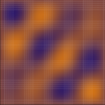
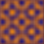
Boots and Tiefelsdorf (2000) showed that (1) the (standardized) spectrum of comprises the possible values for , and (2) the eigenvectors comprise all possible mutually distinct patterns of clustering residual to and accounting for . The positive (negative) eigenvalues of correspond to varying degrees of positive (negative) spatial dependence, and the eigenvectors associated with a given eigenvalue (, say) are the patterns of spatial clustering that data exhibit when the dependence among them is of degree . In other words, the eigenvectors of form a multiresolutional spatial basis for that exhausts all possible patterns that can arise on . Three Moran basis vectors are shown in Figure 1.
 |
 |
 |
Since we do not expect to observe repulsion in the phenomena to which these models are usually applied, we can use the spectrum of the operator to discard all repulsive patterns, retaining only attractive patterns for our analysis (although it can be advantageous to accommodate repulsion (Griffith, 2006)). By retaining only eigenvectors that exhibit positive spatial dependence, we can usually reduce the model dimension by at least half a priori. And Hughes and Haran (2013) showed that a much greater reduction is possible in practice, with 50–100 eigenvectors being sufficient for most datasets. Moreover, a simple spherical Gaussian proposal distribution for performs well because the elements of are approximately a posteriori uncorrelated owing to the orthogonality of the Moran basis.
Although using a truncated Moran basis dramatically reduces the time required to draw samples from the posterior, and the space required to store those samples, this approach does incur the substantial up-front burden of computing and eigendecomposing . The efficiency of the former can be increased by storing in a sparse format (Furrer and Sain, 2010) and parallelizing the matrix multiplications. And we can more efficiently obtain the desired basis vectors by computing only the first eigenvectors of instead of doing the full eigendecomposition. This can be done using the Spectra library (Qiu, 2017), for example.
4.4. Computing for the SCRM
The hierarchical copula model and the direct copula model pose rather different computing challenges. And that is not the only important difference between the two models. A sufficiently substantive discussion of this issue is beyond the scope of this article, but it is worth mentioning that the hierarchical SCRM may be more appealing from a modeling point of view (Musgrove et al., 2016) but suffers from certain limitations when employed as a data-analytic tool (Han and De Oliveira, 2016). For this reason we will focus on copCAR (Hughes, 2015), a form of the direct copula model, here and in Section 5.
copCAR employs the CAR copula, a Gaussian copula (or other suitable copula) based on the proper CAR described above. Recall that the proper CAR has precision matrix , where . Since a copula is scale free, we do not need , but omitting does not leave us with an inverse correlation matrix because the variances are not equal to 1. We could rescale so that its inverse is a correlation matrix, i.e., we could construct a Gaussian copula using , where . In fact, rescaling is necessary in the general case lest the model be unidentifiable with respect to the variances. For copCAR, however, rescaling is unnecessary because the variances are not free parameters; the variances are entirely determined by ’s only dependence parameter, , which is not a scale parameter. Since using itself leads to an identifiable model, rescaling would merely slow computation. Thus copCAR employs the CAR correlation structure indirectly, by using along with the variances . This leads to the CAR copula:
| (10) |
where denotes the distribution function of the normal distribution with mean 0 and variance .
The model specification can be completed by pairing the CAR copula with a set of suitable marginal distributions for the outcomes. The copula and the marginals are linked by way of the probability integral transform. Specifically, if are the observations, and are the desired marginal distribution functions, we have , where is a realization of the copula. We will assume Bernoulli marginal distributions with expectations .
Unless is quite small, computation of the copCAR likelihood is infeasible (when the marginals are discrete) because the multinormal cdf is unstable in high dimensions and because the likelihood contains a sum of terms. For Bernoulli marginals, a composite marginal likelihood approach (Varin, 2008) performs well. The objective function is a product of pairwise likelihoods:
where denotes the bivariate Gaussian copula with covariance matrix
This implies the log composite likelihood
| (11) |
where and . Optimization of (11) yields .
While tends to be approximately normally distributed, tends to be left skewed when is close to 1. This implies that asymptotic inference for tends to result in poor coverage rates. This can be avoided by using a parametric bootstrap, but a parametric bootstrap is rather burdensome computationally. Luckily, a simple reparameterization yields an approximately normally distributed estimator because the objective function for the reparameterized model is approximately quadratic with constant Hessian (Geyer, 2013). Specifically, for , we have
where is the Fisher information matrix and is the variance of the score:
Note that the asymptotic covariance matrix for the CML estimator is a Godambe information matrix (Godambe, 1960) because is misspecified. The matrix can be estimated in the same manner as we described above for the autologistic model.
The form of given in (11) requires four evaluations of the bivariate normal cdf for each of the pairs of observations. This computation is rather expensive even for fairly small samples.
In a spatial setting we can expect a pair of nearby observations to carry more information about dependence than a pair of more distant observations. Others have found, in a variety of contexts, that retaining the contributions to the CML made by more distant pairs of observations decreases not only the computational efficiency of the procedure but also the statistical efficiency of the estimator (Varin and Vidoni, 2009; Apanasovich et al., 2008). Hence, we allow only pairs of adjacent observations to contribute to the copCAR CML. This means replacing (11) with
| (12) |
If thoughtfully implemented, optimization of (12) is efficient enough to permit analysis of larger areal datasets.
5. Application of Various Spatial Regression Models to Simulated Binary Data
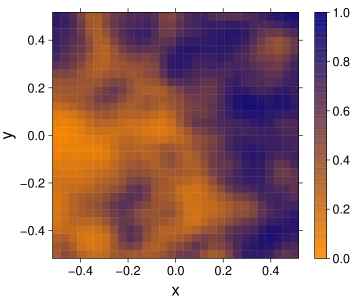
Our simulation study focused on binary areal outcomes, for the reasons given above. We simulated those outcomes on the square lattice. This data size kept the computational burden manageable while giving all of the approaches a fighting chance at performing well. Our mean surface was a function of the and coordinates of the lattice points, and , respectively, which we restricted to the unit square centered at the origin. While simulating data we used linear predictor , where and . Vector exhibits a smaller-scale spatial pattern than do and ; this lends more interesting spatial structure to the mean surface and ensures that and are substantially, but not strongly, correlated ( rather than 0.71). We let , which implies a mean vector equal to
These means are shown in Figure 2.
Predictor was our unmeasured confounder and source of extra- spatial variation. That is, we analyzed the data using , which implies that . More specifically, to each of 100 simulated datasets we applied six models:
-
(1)
the ordinary logistic regression model with linear predictor ;
-
(2)
the centered autologistic model having regression component ;
-
(3)
the copCAR model with marginals;
-
(4)
the traditional CAR model having regression component ;
-
(5)
the sparse RSR model of Hughes and Haran, having regression component and using the first eigenvectors of , where ; and
-
(6)
the sparse RSR model of Hughes and Haran along with the posterior predictive approach of Hanks et al.
The results are provided in Table 1. We see that the RSR approach of Hughes and Haran performed better than the other approaches. The RSR estimator of has the smallest bias and mean squared error, and strikes the best balance between coverage rate and type II error rate. The RSR model also offers the most accurate prediction. The traditional CAR model, along with the RSR approach of Hanks et al., resulted in very high coverage rates at the cost of very high type II error rates. The other three models performed poorly with respect to coverage rate and prediction.
| Model | Med. Est. of | Med. CI Width | MSE | Coverage Rate Type II Rate | Med. |
|---|---|---|---|---|---|
| Ordinary Logistic | 2.11 | 0.97 | 1.29 | 0% 0% = 0 | 4.93 |
| Centered Autologistic | 2.17 | 1.17 | 1.44 | 0% 0% = 0 | 4.18 |
| copCAR | 2.15 | 1.26 | 1.36 | 0% 0% = 0 | 4.93 |
| Traditional CAR | 2.35 | 5.27 | 2.59 | 99% 61% = 38 | 3.21 |
| RSR () | 2.01 | 2.30 | 1.18 | 56% 2% = 54 | 3.01 |
| Adjusted RSR () | 2.01 | 5.75 | 3.51 | 100% 91% = 9 | 3.01 |
Predictions for a single dataset are shown in Figure 3. The autologistic model and the CAR model clearly undersmooth. The CAR model’s undersmoothing is less dramatic, but it is perhaps surprising that the CAR model undersmoothes at all given that it has spatial random effects. (Note that we could force to be smoother by using in place of (Rue and Held, 2005).)
| RSR () | |
 |
 |
| CAR | Autologistic |
 |
 |
6. Bayesian Spatial Filtering
In this section we will develop, and assess the performance of, Bayesian spatial filtering, which possesses the computational advantages and good predictive performance of RSR while allowing for some advantages in regression inference. We begin by describing classical spatial filtering.
6.1. Classical Spatial Filtering
In developing the SAMM, Hughes and Haran (2013) drew inspiration from spatial filtering (Griffith, 2003), which uses a basis expansion to accommodate any extra- spatial pattern exhibited by the response vector, resulting in conventional residuals, i.e., residuals having at most trace spatial dependence. This implies that spatial filtering can reveal extra- structure while permitting the analyst to apply ordinary, well-understood diagnostic techniques to the residuals.
The basis used most often in spatial filtering are eigenvectors of the Moran operator for : . This yields vectors that reside in . (Recall that the SAMM employs basis vectors from , where typically contains along with one or more spatially structured predictors.) Considerable dimension reduction can be achieved by using only basis vectors. If we store said vectors as the columns of matrix , say, the filtering linear predictor can be written as
where is once again a -vector of coefficients.
Since constructing requires that be computed and eigendecomposed, it is clear that spatial filtering and the SAMM have much in common from a computational point of view. There are two key differences, however. First, to our knowledge, there are no Bayesian approaches for spatial filtering; practitioners estimate by optimizing a likelihood or a composite likelihood. The choice of objective function of course has a substantial impact on computational complexity. And second, the columns of can be chosen using any of a number of methods (three will be discussed shortly). Those methods vary greatly in sophistication and computational complexity. It is not clear how they compare to one another with respect to quality of regression inference or quality of prediction, however.
Chun et al. (2016) recommend that the first
eigenvectors be included initially in a stepwise, ordinary GLM analysis with a significance level of 0.2. Here, is the number of positive eigenvalues of and is the score of Moran’s for the response.
For a binary response, another possibility is to do a two-sample test for each of the first few hundred eigenvectors, where the eigenvector of interest is treated as the response and is used as the grouping variable. Any eigenvector that yields a -value smaller than 0.1, say, is then included in the analysis. In this scheme, the number of variables may or may not be further reduced using a stepwise procedure.
A third approach to spatial filtering is to include Moran eigenvectors in a spatial model and use that model’s dependence component to decide which eigenvectors to retain. For example, one might use some procedure to choose the Moran eigenvectors that lead to for an appropriate automodel, or for a model that employs the proper CAR. It is this technique for which spatial filtering is named, since here an explicit aim is to remove (filter) spatial dependence from the response (Griffith, 2004).
6.2. A Bayesian Approach to Spatial Filtering
We can develop a Bayesian approach to spatial filtering by replacing in the SAMM specification with a filtering design matrix . Specifically, the Bayesian spatial filtering (BSF) model has the same transformed conditional mean as the classical spatial filtering model, namely,
where contains the principle eigenvectors of , and is a -vector of coefficients. Borrowing from the SAMM, the prior distribution for is
| (13) |
where is once again the Laplacian of . The BSF model, like the SAMM, assigns a spherical Gaussian prior with a large variance, and assigns the smoothing parameter a gamma prior with shape parameters 0.5 and 2,000. Note that the latter prior, having a large mean, discourages artifactual spatial structure in the posterior (Kelsall and Wakefield, 1999).
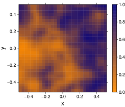
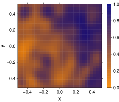
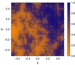
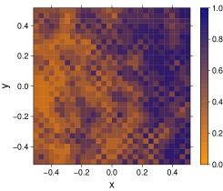
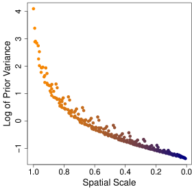
Since are regression coefficients, one may be tempted to assign a spherical Gaussian prior instead of the above mentioned prior. This would be a mistake, however, for (13) is not arbitrary (see Reich et al. (2006) and/or Hughes and Haran (2013) for derivations) but is, in fact, very well suited to the task at hand. Specifically, two characteristics of (13)—along with the above mentioned prior for —discourage overfitting even when is too large for the dataset being analyzed. First, the prior variances are commensurate with the spatial scales of the predictors in (Figure 4). This shrinks toward zero the coefficients corresponding to predictors that exhibit small-scale spatial variation. Additionally, the correlation structure of (13) effectively reduces the degrees of freedom in the smoothing component of the model.
If the response is non-Gaussian, and are updated using Metropolis–Hastings random walks with Gaussian proposals. The proposal covariance matrix for is the estimated asymptotic covariance matrix from an ordinary GLM fit to the data, which generally yields an acceptance rate around 50%. The proposal for is spherical Gaussian—with standard deviation , say. A sensible default value for is 0.1, but a smaller value may be required to achieve large enough acceptance rates for larger datasets. The update for is a Gibbs update irrespective of the response distribution. If the response is Gaussian distributed, all updates are Gibbs updates. Note that the BSF MCMC sampler is very easy to tune since is the only tuning parameter (unless the outcomes are Gaussian, in which case no tuning is required).
Bayesian spatial filtering for point-level outcomes can be accomplished analogously by adapting Guan and Haran’s (2016) random-projection framework. The resulting BSF model for point-level data is different from the areal BSF model in a potentially important way, however. Since Guan and Haran obtain their basis vectors by eigendecomposing , they, quite naturally, assign a spherical Gaussian prior to . Because a spherical Gaussian prior lacks the appealing attributes of (13), Guan and Haran recommend that be chosen in a pre-processing step. It is not clear how well this approach performs compared to the use of a prior similar to (13).
6.3. Application of BSF to Simulated Binary Data
As a followup to the simulation study described in Section 5, we applied our BSF model to the simulated datasets. We used four different values for : 50, 100, 200, and 400. The results are given in Table 2.
For smaller values of , has smaller bias and MSE than any of the other estimators considered here, and yields a higher coverage rate while keeping the type II rate very low. As becomes large, the bias and MSE of grow. Eventually the coverage rate begins to decrease, the type II rate to increase. The BSF model also performs very well at prediction.
The BSF model accomplishes all of this through judicious use of multicollinearity. Recall that the basis vectors used in RSR are (at least nearly) uncorrelated with the columns of . This is not the case for the BSF model since spatial filtering employs eigenvectors of . As we increase , we introduce more and more multicollinearity between and . Up to a point, this alleviates unmeasured confounding to some extent (hence the reduced bias), and adjusts the variance upward by a modest amount (hence the increased coverage rate). As gets large, the linear predictor becomes rather redundant, causing the BSF model to perform much like the CAR model (increased bias and type II error rate).
| Model | Med. Est. of | Med. CI Width | MSE | Coverage Rate Type II Rate | Med. |
|---|---|---|---|---|---|
| Ordinary Logistic | 2.11 | 0.97 | 1.29 | 0% 0% = 0 | 4.93 |
| Centered Autologistic | 2.17 | 1.17 | 1.44 | 0% 0% = 0 | 4.18 |
| copCAR | 2.15 | 1.26 | 1.36 | 0% 0% = 0 | 4.93 |
| Traditional CAR | 2.35 | 5.27 | 2.59 | 99% 61% = 38 | 3.21 |
| RSR () | 2.01 | 2.30 | 1.18 | 56% 2% = 54 | 3.01 |
| Adjusted RSR () | 2.01 | 5.75 | 3.51 | 100% 91% = 9 | 3.01 |
| BSF () | 1.87 | 2.08 | 0.94 | 63% 2% = 61 | 3.07 |
| BSF () | 1.89 | 2.34 | 0.96 | 74% 2% = 72 | 3.01 |
| BSF () | 1.99 | 2.69 | 1.25 | 81% 2% = 79 | 2.99 |
| BSF () | 2.25 | 3.23 | 1.88 | 67% 20% = 47 | 3.01 |
7. Conclusion
When unmeasured confounding is the source of extra- spatial variation in a response variable, spatial regression models struggle to perform well. In Section 5 we saw that the autologistic model and the copCAR model (examples of the automodel and the spatial copula regression model, respectively) perform rather poorly, about as poorly as a non-spatial model. Spatial mixed-effects models perform better but still have weaknesses. The traditional SGLMM, for example, is badly spatially confounded and computationally burdensome, and often undersmoothes. Restricted spatial regression offers an appealing alternative, for RSR reduces bias and mean squared error, provides a more sensible balance between coverage rate and type II rate, smoothes very effectively, and permits efficient computation. Yet there is room for improvement.
In the latter part of this article we developed Bayesian spatial filtering, which performs as well as RSR with respect to prediction and computational complexity while besting RSR in terms of bias, mean squared error, and coverage rate. BSF does this by using an expansion in a well-chosen basis to introduce an appropriate amount of spatial confounding. This situates the BSF model on a continuum of spatial confounding, with the non-spatial model and the CAR model at either end:
References
- Apanasovich et al. (2008) Apanasovich, T., Ruppert, D., Lupton, J., Popovic, N., Turner, N., Chapkin, R., and Carroll, R. (2008). Aberrant crypt foci and semiparametric modeling of correlated binary data. Biometrics, 64(2):490–500.
- Assunção and Krainski (2009) Assunção, R. and Krainski, E. (2009). Neighborhood dependence in Bayesian spatial models. Biometrical Journal, 51(5):851–869.
- Banerjee et al. (2013) Banerjee, A., Dunson, D. B., and Tokdar, S. T. (2013). Efficient Gaussian process regression for large datasets. Biometrika, 100(1):75.
- Banerjee et al. (2014) Banerjee, S., Carlin, B., and Gelfand, A. (2014). Hierarchical Modeling and Analysis for Spatial Data. Chapman & Hall/CRC, Boca Raton.
- Banerjee et al. (2008) Banerjee, S., Gelfand, A., Finley, A., and Sang, H. (2008). Gaussian predictive process models for large spatial data sets. Journal of the Royal Statistical Society: Series B (Statistical Methodology), 70(4):825–848.
- Besag (1974) Besag, J. (1974). Spatial interaction and the statistical analysis of lattice systems (with discussion). Journal of the Royal Statistical Society, Series B: Methodological, 36:192–236.
- Besag (1975) Besag, J. (1975). Statistical analysis of non-lattice data. The Statistician: Journal of the Institute of Statisticians, 24:179–196.
- Besag et al. (1991) Besag, J., York, J., and Mollié, A. (1991). Bayesian image restoration, with two applications in spatial statistics (Disc: P21-59). Annals of the Institute of Statistical Mathematics, 43:1–20.
- Boots and Tiefelsdorf (2000) Boots, B. and Tiefelsdorf, M. (2000). Global and local spatial autocorrelation in bounded regular tessellations. Journal of Geographical Systems, 2(4):319.
- Brouwer and Haemers (2012) Brouwer, A. E. and Haemers, W. H. (2012). Spectra of Graphs. Springer-Verlag.
- Byrd et al. (1995) Byrd, R., Lu, P., Nocedal, J., and Zhu, C. (1995). A limited memory algorithm for bound constrained optimization. SIAM Journal on Scientific Computing, 16(5):1190–1208.
- Caragea and Kaiser (2009) Caragea, P. and Kaiser, M. (2009). Autologistic models with interpretable parameters. Journal of Agricultural, Biological, and Environmental Statistics, 14(3):281–300.
- Chun et al. (2016) Chun, Y., Griffith, D. A., Lee, M., and Sinha, P. (2016). Eigenvector selection with stepwise regression techniques to construct eigenvector spatial filters. Journal of Geographical Systems, 18(1):67–85.
- Clayton et al. (1993) Clayton, D., Bernardinelli, L., and Montomoli, C. (1993). Spatial correlation in ecological analysis. International Journal of Epidemiology, 22(6):1193–1202.
- Clifford (1990) Clifford, P. (1990). Markov random fields in statistics. In Grimmett, G. R. and Welsh, D. J. A., editors, Disorder in Physical Systems: A Volume in Honour of John M. Hammersley on His 70th Birthday, pages 19–32. Clarendon Press [Oxford University Press].
- Cressie and Johannesson (2008) Cressie, N. and Johannesson, G. (2008). Fixed rank kriging for very large spatial data sets. Journal of the Royal Statistical Society: Series B (Statistical Methodology), 70(1):209–226.
- Cressie (1993) Cressie, N. A. (1993). Statistics for Spatial Data. John Wiley & Sons, New York, 2nd. edition.
- Datta et al. (2016) Datta, A., Banerjee, S., Finley, A. O., and Gelfand, A. E. (2016). Hierarchical nearest-neighbor Gaussian process models for large geostatistical datasets. Journal of the American Statistical Association, 111(514):800–812.
- De Oliveira (2000) De Oliveira, V. (2000). Bayesian prediction of clipped Gaussian random fields. Computational Statistics & Data Analysis, 34(3):299–314.
- Diggle et al. (1998) Diggle, P. J., Tawn, J. A., and Moyeed, R. A. (1998). Model-based geostatistics (Disc: P326-350). Journal of the Royal Statistical Society, Series C: Applied Statistics, 47:299–326.
- Efron and Tibshirani (1994) Efron, B. and Tibshirani, R. J. (1994). An Introduction to the Bootstrap. CRC Press.
- Furrer et al. (2006) Furrer, R., Genton, M., and Nychka, D. (2006). Covariance tapering for interpolation of large spatial datasets. Journal of Computational and Graphical Statistics, 15(3):502–523.
- Furrer and Sain (2010) Furrer, R. and Sain, S. R. (2010). spam: A sparse matrix R package with emphasis on MCMC methods for Gaussian Markov random fields. Journal of Statistical Software, 36(10):1–25.
- Gelman et al. (2013) Gelman, A., Carlin, J. B., Stern, H. S., Dunson, D. B., Vehtari, A., and Rubin, D. B. (2013). Bayesian Data Analysis. Chapman and Hall/CRC, third edition.
- Geyer (2013) Geyer, C. J. (2013). Le Cam made simple: Asymptotics of maximum likelihood without the LLN or CLT or sample size going to infinity. In Jones, G. L. and Shen, X., editors, Advances in Modern Statistical Theory and Applications: A Festschrift in honor of Morris L. Eaton. Institute of Mathematical Statistics, Beachwood, Ohio, USA.
- Godambe (1960) Godambe, V. (1960). An optimum property of regular maximum likelihood estimation. The Annals of Mathematical Statistics, pages 1208–1211.
- Griffith (2004) Griffith, D. (2004). A spatial filtering specification for the autologistic model. Environment and Planning A, 36(10):1791–1811.
- Griffith (2003) Griffith, D. A. (2003). Spatial Autocorrelation and Spatial Filtering: Gaining Understanding Through Theory and Scientific Visualization. Springer, Berlin.
- Griffith (2006) Griffith, D. A. (2006). Hidden negative spatial autocorrelation. Journal of Geographical Systems, 8(4):335–355.
- Guan and Haran (2016) Guan, Y. and Haran, M. (2016). A computationally efficient projection-based approach for spatial generalized linear mixed models. ArXiv e-prints.
- Halko et al. (2011) Halko, N., Martinsson, P.-G., and Tropp, J. A. (2011). Finding structure with randomness: Probabilistic algorithms for constructing approximate matrix decompositions. SIAM Review, 53(2):217–288.
- Han and De Oliveira (2016) Han, Z. and De Oliveira, V. (2016). On the correlation structure of Gaussian copula models for geostatistical count data. Australian & New Zealand Journal of Statistics.
- Hanks et al. (2015) Hanks, E. M., Schliep, E. M., Hooten, M. B., and Hoeting, J. A. (2015). Restricted spatial regression in practice: Geostatistical models, confounding, and robustness under model misspecification. Environmetrics, 26(4):243–254.
- Haran (2011) Haran, M. (2011). Gaussian random field models for spatial data. Handbook of Markov Chain Monte Carlo, pages 449–478.
- Haran et al. (2003) Haran, M., Hodges, J., and Carlin, B. (2003). Accelerating computation in Markov random field models for spatial data via structured MCMC. Journal of Computational and Graphical Statistics, 12(2):249–264.
- Haran and Tierney (2010) Haran, M. and Tierney, L. (2010). On automating Markov chain Monte Carlo for a class of spatial models. Bayesian Analysis, pages 1–26.
- Higdon (2002) Higdon, D. (2002). Space and space-time modeling using process convolutions. In Anderson, C., Barnett, V., Chatwin, P., and El-Shaarawi, A., editors, Quantitative Methods for Current Environmental Issues, pages 37–56. Springer-Verlag, London.
- Hodges and Reich (2010) Hodges, J. S. and Reich, B. J. (2010). Adding spatially-correlated errors can mess up the fixed effect you love. The American Statistician, 64(4):325–334.
- Hughes (2014) Hughes, J. (2014). ngspatial: A package for fitting the centered autologistic and sparse spatial generalized linear mixed models for areal data. The R Journal, 6(2):81–95.
- Hughes (2015) Hughes, J. (2015). copCAR: A flexible regression model for areal data. Journal of Computational and Graphical Statistics, 24(3):733–755.
- Hughes and Haran (2013) Hughes, J. and Haran, M. (2013). Dimension reduction and alleviation of confounding for spatial generalized linear mixed models. Journal of the Royal Statistical Society: Series B (Statistical Methodology), 75(1):139–159.
- Hughes et al. (2011) Hughes, J., Haran, M., and Caragea, P. C. (2011). Autologistic models for binary data on a lattice. Environmetrics, 22(7):857–871.
- Joe (2014) Joe, H. (2014). Dependence Modeling with Copulas. Chapman and Hall/CRC, Boca Raton, USA.
- Kaiser and Cressie (1997) Kaiser, M. S. and Cressie, N. (1997). Modeling Poisson variables with positive spatial dependence. Statistics & Probability Letters, 35:423–432.
- Kazianka and Pilz (2010) Kazianka, H. and Pilz, J. (2010). Copula-based geostatistical modeling of continuous and discrete data including covariates. Stochastic Environmental Research and Risk Assessment, 24(5):661–673.
- Kelsall and Wakefield (1999) Kelsall, J. and Wakefield, J. (1999). Discussion of “Bayesian models for spatially correlated disease and exposure data”, by Best et al. In Bernardo, J., Berger, J., Dawid, A., and Smith, A., editors, Bayesian Statistics 6. Oxford University Press, New York.
- Kindermann and Snell (1980) Kindermann, R. and Snell, J. (1980). Markov Random Fields and Their Applications. American Mathematical Society, Providence, RI.
- Knorr-Held and Rue (2002) Knorr-Held, L. and Rue, H. (2002). On block updating in Markov random field models for disease mapping. Scandinavian Journal of Statistics, 29(4):597–614.
- Kolev and Paiva (2009) Kolev, N. and Paiva, D. (2009). Copula-based regression models: A survey. Journal of Statistical Planning and Inference, 139(11):3847–3856.
- Lindgren et al. (2011) Lindgren, F., Rue, H., and Lindström, J. (2011). An explicit link between Gaussian fields and Gaussian Markov random fields: the stochastic partial differential equation approach. Journal of the Royal Statistical Society: Series B (Statistical Methodology), 73(4):423–498.
- Lindsay (1988) Lindsay, B. (1988). Composite likelihood methods. Contemporary Mathematics, 80(1):221–239.
- McCullagh and Nelder (1983) McCullagh, P. and Nelder, J. A. (1983). Generalized Linear Models. Chapman & Hall Ltd.
- Moran (1950) Moran, P. (1950). Notes on continuous stochastic phenomena. Biometrika, 37(1/2):17–23.
- Musgrove et al. (2016) Musgrove, D., Hughes, J., and Eberly, L. (2016). Hierarchical copula regression models for areal data. Spatial Statistics, 17:38–49.
- Paciorek (2010) Paciorek, C. J. (2010). The importance of scale for spatial-confounding bias and precision of spatial regression estimators. Statistical Science: A Review Journal of the Institute of Mathematical Statistics, 25(1):107.
- Park and Haran (2017) Park, J. and Haran, M. (2017). Bayesian inference in the presence of intractable normalizing functions. ArXiv e-prints.
- Qiu (2017) Qiu, Y. (2017). Spectra: Sparse eigenvalue computation toolkit as a redesigned ARPACK.
- Rasmussen and Williams (2006) Rasmussen, C. and Williams, C. (2006). Gaussian Processes for Machine Learning. Springer.
- Reich et al. (2006) Reich, B., Hodges, J., and Zadnik, V. (2006). Effects of residual smoothing on the posterior of the fixed effects in disease-mapping models. Biometrics, 62(4):1197–1206.
- Rue and Held (2005) Rue, H. and Held, L. (2005). Gaussian Markov Random Fields: Theory and Applications, volume 104 of Monographs on Statistics and Applied Probability. Chapman & Hall, London.
- Rue et al. (2009) Rue, H., Martino, S., and Chopin, N. (2009). Approximate Bayesian inference for latent Gaussian models by using integrated nested Laplace approximations. Journal of the Royal Statistical Society: Series B (Statistical Methodology), 71(2):319–392.
- Rue and Tjelmeland (2002) Rue, H. and Tjelmeland, H. (2002). Fitting Gaussian Markov random fields to Gaussian fields. Scandinavian Journal of Statistics, 29(1):31–49.
- Sarlos (2006) Sarlos, T. (2006). Improved approximation algorithms for large matrices via random projections. In Foundations of Computer Science, 2006. FOCS’06. 47th Annual IEEE Symposium on, pages 143–152. IEEE.
- Varin (2008) Varin, C. (2008). On composite marginal likelihoods. AStA Advances in Statistical Analysis, 92(1):1–28.
- Varin et al. (2011) Varin, C., Reid, N., and Firth, D. (2011). An overview of composite likelihood methods. Statistica Sinica, 21(1):5–42.
- Varin and Vidoni (2009) Varin, C. and Vidoni, P. (2009). Pairwise likelihood inference for general state space models. Econometric Reviews, 28, 1(3):170–185.
- Wall (2004) Wall, M. M. (2004). A close look at the spatial structure implied by the CAR and SAR models. Journal of Statistical Planning and Inference, 121(2):311–324.