Stochastic Modeling and Simulation of Viral Evolution

Abstract

RNA viruses comprise vast populations of closely related, but highly genetically diverse, entities known as quasispecies. Understanding the mechanisms by which this extreme diversity is generated and maintained is fundamental when approaching viral persistence and pathobiology in infected hosts. In this paper we access quasispecies theory through a mathematical model based on the theory of multi-type branching processes, to better understand the roles of mechanisms resulting in viral diversity, persistence and extinction. We accomplish this understanding by a combination of computational simulations and the theoretical analysis of the model. In order to perform the simulations we have implemented the mathematical model into a computational platform capable of running simulations and presenting the results in a graphical format in real time. Among other things, we show that the establishment of virus populations may display four distinct regimes from its introduction into new hosts until achieving equilibrium or undergoing extinction. Also, we were able to simulate different fitness distributions representing distinct environments within a host which could either be favorable or hostile to the viral success. We addressed the most used mechanisms for explaining the extinction of RNA virus populations called lethal mutagenesis and mutational meltdown. We were able to demonstrate a correspondence between these two mechanisms implying the existence of a unifying principle leading to the extinction of RNA viruses.

1 Introduction

Viruses with RNA genomes, the most abundant group of human pathogens DH97 , exhibit high mutational rates, fast replicative kinetics, large population sizes, and high genetic diversity. Current evidences also indicate that RNA virus populations consist of a wide and interrelated distribution of variants, which can display complex evolutionary dynamics. The complex evolutionary properties of RNA virus populations features the modulation of viral phenotypic traits, the interplay between host and viral factors, and other emergent properties D85 ; DMP06 . During viral infections, these features allow viral populations to escape from host pressures represented by the actions from the immune system, from vaccines and to develop resistance antiviral drugs. Taken together these features represent the major obstacle for the success and implementation of effective therapeutic intervention strategies.

In order o describe the evolution of RNA viruses and its relationship with their hosts and antiviral therapies, theoretical models of virus evolution have been developed. These models employ mathematical and computational tools as methodological instruments allowing one to address evolutionary questions from a different perspective than the commonly seen use of modern experimental technologies. This kind of approach allows the implementation of low-cost research projects addressing evolutionary questions that are usually investigated by experimental methods. At a deeper level, they provide a systematic perspective of the biological phenomenon, when viewed as proof-of-concept models SBD14 . Verbal or pictorial models have long been used in evolutionary biology to formulate abstract hypotheses about processes and mechanisms that operate among diverse species and across vast time scales. Used in many fields, proof-of-concept-models test the validity of verbal or pictorial models by laying out the underlying assumptions in a mathematical framework.

Eigen and Schuster E71 ; ES79 proposed and analyzed a deterministic model for the evolution of polynucleotides in a dialysis reactor based on a system of ordinary, differential equations called quasispecies model. Subsequently, Demetrius et al. DSS85 proposed a stochastic quasispecies model in order to overcome some drawbacks of the deterministic quasispecies model of Eigen and Schuster ES79 . The approach of Demetrius et al. DSS85 employed very powerful methods based on the theory of stochastic branching processes. This theory, originally developed to deal with the extinction of family names (Watson and Galton WG1874 ), has been applied since the forties to a great variety of physical and biological problems H63 ; AN72 ; K02 . On the experimental side, an early study of the RNA phage $\mathrm{Q\beta}$ reporting that sequence variation in a population was high but approximately stable over time around a consensus sequence, gave the initial stimulus to consider the notion of quasispecies in the broader context of RNA viruses DSTW78 .

Since then, quasispecies theory has been recognized as a subset of theoretical population genetics W05 ; TH07 . Recently, in the series of papers C15a ; C15b ; D15 ; CD16 , it has been rigorously shown that the Wright-Fisher and Moran models for multi-loci mutation-selection converges to the single-peak fitness landscape quasispecies model, in the appropriate limit of infinite populations. Moreover, due to is a capability to accommodate high mutation rates, it has been widely applied to model the evolution of viruses with RNA genomes E93 .

Inspired by the stochastic quasispecies model of Demetrius et al. DSS85 and based on branching process techniques, Antoneli et al. ABCJ13b ; ABCJ13a proposed a mathematical model aimed at understanding the basic mechanisms and phenomena of the evolution of highly-mutating viral populations replicating in a single host organism, called phenotypic (quasispecies) model. It is denominated “phenotypic” due to the fact that it only comprises probabilities associated with the occurrence of deleterious, beneficial and neutral effects that operate directly on the replicative capability of viral particles, without any explicit reference to their genome. In D16 Dalmau introduced another generalization of the stochastic quasispecies model also based on multitype branching processes but retaining the genotypic character of Demetrius et al. DSS85 .

The phenotypic model ABCJ13b ; ABCJ13a is defined through a probability generating function which formally determines the transition structure of the process. The matrix of first moments of the branching process, or simply the mean matrix, defines a deterministic linear system which describes the time evolution of conditional expectations, a “mean field model” for the actual stochastic process which is equivalent to the Eigen’s selection equation DSS85 . The deterministic mean field model has been studied by several researches, but without the connection to a stochastic branching process, see for instance BMR99 ; MLPED03 ; C11 .

As shown in ABCJ13b ; ABCJ13a , the phenotypic model is fully specified by three fundamental parameters: the probabilities of occurrence of deleterious and beneficial effects $d$ and $b$ – the probability of occurrence of neutral effects is fixed by the complementary relation $c=1-d-b$ – and the maximum replicative capability $R$. By an exhaustive analysis of this “parameter space” we were able to depict a fairly detailed portrait of all possible behaviors of the model. In ABCJ13b we carry out a thorough analysis of mean matrix, assuming that beneficial effects are absent and were able to show that the phenotypic model is “exactly solvable”, in the sense that the spectral problem for the mean matrix has an explicit solution. In ABCJ13a we employ spectral perturbation theory in order to treat the general case of small beneficial effects. This approach has provided a complete description of the generic behavior of the model.

In the present paper, we further address the biological implications of modeling RNA virus populations in terms of the phenotypic model. We achieved this goal by a combination of computational simulations and basic results of the theory of multitype branching processes as used in ABCJ13b ; ABCJ13a . In order to perform the simulations we have implemented the phenotypic model into a computational platform capable of running the simulation and presenting the results in graphical format in real time.

We start with the description of the computational platform (its interface, output and main simulation routine). Then we proceed to use some of the theoretical results of ABCJ13b ; ABCJ13a to validate the program with several simulation experiments that can be read independently from each other and are used to evaluate distinct features of the program. Finally, we perform two additional simulation experiments to address the main questions of this paper:

1. What is the impact of fitness distributions on the evolution of the phenotypic model and how to measure it?

2. Is there an extinction mechanism similar to the “mutational meltdown” in the phenotypic model?

Role of fitness distributions.

The fitness distributions of the phenotypic model are discrete distributions forming location-scale families parameterized by the replicative classes that control the progeny sizes at each replication cycle. They can be seen as representing distinct “compartments” in the host which can be more favorable or pose restrictions to the viral replication process. For instance, some distributions have a positive influence on the replication, by enhancing the replication of particles in the higher replicative classes, while other distributions have an opposite effect. Examples of favorable compartments would be sites associated with immune privilege, or with lower concentration of antiviral drugs, or allowing for cell to cell virus transmission. Unfavorable compartments are sites with high antiviral drug penetration, small number of target cells, or accessed by elements of host responses as antibodies, citotoxic cells and others. In this sense, we may think of fitness distributions as an environmental component during viral evolution. We show that the impact of the fitness distributions on the branching process is subtle and can not be detected by quantities that depend only on the first moments of the process. Nevertheless, we introduce a new quantity, called populational variance, that is capable to detect the influence of different fitness distributions and is analytically and computationally tractable.

Unifying principle for extinction.

According to the phenotypic model a virus population can be become extinct or eradicated from the host by the fulfillment of a condition involving only the probability of occurrence of deleterious effects $d$ and the maximum replicative capability $R$. Even further, in the absence of beneficial or compensatory effects, the fate of the population determined by the product $R(1-d)$. If it is greater than $1$ the population will survive or if it is lesser than $1$ the population will face extinction. Based on this result we show that there is a correspondence between two well known distinct mechanisms of extinction:

1. Lethal Mutagenesis LEKZRM99 ; BSW07 ; BSW08 . The process of extinction of the viral population due to the increment of the deleterious rate.

2. Mutational Meltdown LBBG93 ; LG90 . The process of extinction of the viral population through the step-wise loss of the fittest replicative classes due to random drift associated with the finite population size effect.

The correspondence between the two mechanisms reinforces the view that both are “two sides of the same coin” MOBJ17 . We propose here an unifying principle for the extinction of a virus population: This principle is based on a mathematical model containing probabilities of neutral and deleterious effects and the average growth rate or average maximum fitenss which is equivalent (under appropriate interpretation) to the extinction threshold of a branching process given by the malthusian parameter. In the course of the proof (see Section 3.3) we consider another parameter present in our phenotypic model, called the carrying capacity. Initially, it was introduced as a convenient step for the computational implementation of the model, i.e., to prevent the population to grow boundlessly. Nevertheless, it can be seen as a genuine parameter of the model, which controls the intensity of the random drift. Because of this, we may consider our model as a self-regulated branching process, instead of a “pure” branching process. Furthermore, we observe that, even though the extinction mechanisms have the same mathematical “origin”, the processes leading to the actual extinction of the viral population may display distinct “signatures”.

Structure of the paper.

The paper is structured as follows. In section 2 we introduce the computational platform for the simulation of the phenotypic model. In section 3 we perform several simulation experiments to validate the program by comparing its output with the theoretical results from ABCJ13b ; ABCJ13a . We end this section with the presentation of the new results on the role of the fitness distributions and the mutational meltdown. The validation subsections and the two subsections on new results depend only on section 2 and so can be read independently from each other. The paper ends with a conclusion section. There are 5 appendices. Appendices A, B and C provide some background on branching process theory and theoretical results about the phenotypic model for the reader’s convenience. Appendices D and E provide some details about the implementation of the computational platform introduced in the paper.

2 Software Description

In this section introduce a computational platform for the simulation of the phenotypic model of ABCJ13b ; ABCJ13a .

2.1 The ENVELOPE Program

The ENVELOPE (EvolutioN of Virus populations modELd by stOchastic ProcEss) program is a cross-platform application developed to simulate the phenotypic model of ABCJ13b ; ABCJ13a . The software contains a graphical interface to input data, visualize graphics in real time, and export the output data to CSV format, which can be used with a wide range of statistical analysis tools. It was written in C++ programming language using the Qt framework to design the graphical user interface. It was exhaustively tested on Linux operating systems.

The main window of the program has several tabs with the first called “Data Input” where the user can set the values of several parameters that completely specify the model, as follows (see Figure 1).

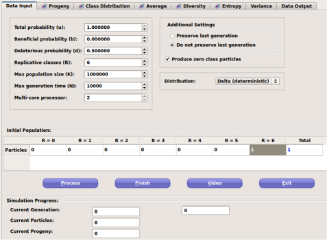
Figure 1: The “Data Input” tab of the ENVELOPE program.

• Total probability ($u$): the probability that a progeny particle will undergo some fitness effect. It should be a number between $0$ and $1$. The effect of this probability is to renormalize the other probabilities ($p\mapsto u\,p$) and its default value is $u=1$ (no renormalization).

• Beneficial probability ($b$): the probability of occurrence of a beneficial effect. It should be a number between $0$ and $1$.

• Deleterious probability ($d$): the probability of occurrence of deleterious effect. It should be a number between $0$ and $1$.
  The complementary probability $c=1-b-d$ is the probability of occurrence of neutral effect. If $b+d>1$ then $c$ is set to $0$ and $d=1-b$.

• Replicative classes ($R$): the number of non-zero replicative classes, hence there are $R+1$ replicative classes (maximum replicative capability).

• Max population size ($K$): the maximum population size (carrying capacity).

• Maximum generation time ($N$): the total number of generations to be simulated. Each generation corresponds to a replication cycle.

• Multi-core processor: controls the recruitment of processors by the program.

• Initial population: the number of particles in each replicative class that will initiate the process.

• Distribution: location-scale family of fitness distributions (see Table 1).

Distribution	Family ($r\geqslant 1$)	Variance
Deterministic	$t_{r}(k)=\delta_{rk}$	$0$
Poisson	$t_{r}(k)=\mathrm{e}^{-r}\tfrac{r^{k}}{k!}$	$r$
Geometric	$t_{r}(k)=\tfrac{1}{r+1}\big{(}1-\tfrac{1}{r+1}\big{)}^{k}$	$r(r+1)$
$\tfrac{1}{2}$-Binomial	$t_{r}(k)=\binom{2r}{k}\tfrac{1}{2^{r}}$	$r/2$
Power law	$t_{r}(k)=\mathfrak{z}_{r}(k)$	$+\infty$

Table 1: Location-scale families of fitness distributions. All distributions are normalized so that the expectation value of $t_{r}$ is $r$ and $t_{0}(k)=\delta_{0k}$. See Appendix B for the notation $\delta_{rk}$ and Appendix D for the definition of the family of power law distributions $\mathfrak{z}_{r}(k)$.

The remaining tabs (“Progeny”, “Class Distribution”, “Average”, “Diversity”, “Entropy”, “Variance”) display graphics of the above quantities in real time as the simulation proceeds. The tab “Data Output” displays a table with all the data generated during the simulation. This data can be saved to a file (button “Save to File”) or copied to the memory (button “Copy to Memory”) and then it can be directly pasted into a spreadsheet.

The button “Process” starts the simulation, the button “Finish” ends the simulation at any time and the button “Exit” closes the program. If the total number of particles in a generation is equal to zero, it is assumed that the population has become extinct and hence the simulation stops. The button “Video” pauses the simulation, without ending the simulation, and allows the user to change the above parameter settings and continue the simulation with the new setting. This feature is used to emulate the changes in the environment – the host organism – where the reproduction process takes place.

The evolution of the population can be measured through a few simple quantities that vary as a function of the generation number $n\geqslant 0$. Let $\bm{Z}_{n}=(Z_{n}^{0},\ldots,Z_{n}^{R})$ denote the vector whose component $Z^{r}_{n}$ is the number of particles in the $r$-th replicative class at generation $n$.

• Progeny size: total number of particles $|\bm{Z}_{n}|=\sum_{r}Z^{r}_{n}$ at generation $n$.

• Relative growth rate: the relative growth rate at generation $n$ given by (for $n>1$)

  $$\mu(n)=\dfrac{|\bm{Z}_{n}|}{|\bm{Z}_{n-1}|}$$

  It is a multidimensional version of the Lotka-Nagaev estimator L39 ; N67 , which gives an empirical estimator of the malthusian parameter.

• Asymptotic distribution of classes: the proportion of particles in the $r$-th replicative class at generation $n$ given by

  $$u_{r}(n)=\dfrac{Z^{r}_{n}}{|\bm{Z}_{n}|}$$

  The vector $\bm{u}(n)=\big{(}u_{0}(n),\ldots,u_{R}(n)\big{)}$ is called asymptotic distribution of classes (or simply the class distribution).

• Average reproduction rate: the average reproduction rate (mean of the class distribution) at generation $n$ given by

  $$\langle\varrho(n)\rangle=\sum_{r=0}^{R}r\,u_{r}(n)$$

  It can be shown that the average reproduction rate equals to the relative growth rate:

  $$\langle\varrho(n)\rangle=\mu(n)\qquad\text{for all}\quad n>1$$

  (see Appendix A for details).

• Phenotypic diversity: the variance (or standard deviation) of the class distribution at generation $n$ given by

  $$\sigma_{\varrho}^{2}(n)=\sum_{r=0}^{R}r^{2}\,u_{r}(n)-\langle\varrho(n)\rangle^{2}$$

• Phenotypic entropy: the informational or Shannon entropy of the class distribution at generation $n$ given by

  $$h_{\varrho}(n)=-\sum_{r=0}^{R}u_{r}(n)\,\ln u_{r}(n)$$

  Here we use the convention “$0\ln 0\equiv 0$”. This quantity behaves very much like the phenotypic diversity.

• Normalized populational variance: the normalized populational variance at generation $n$ given by

  $$\phi(n)=\sigma^{2}(n)-\sigma^{2}_{\varrho}(n)$$

  where $\sigma^{2}$ is the empirical estimator of the variance corresponding to the malthusian parameter $\mu(n)$ (see Appendix A for details).

Strictly speaking, a surviving population described by branching process which does not becomes extinct grows indefinitely, at an exponential rate proportional to $\mu^{n}$. Hence, in order to simulate a branching process it is necessary to impose a cut off on the progeny size, otherwise it would blow up the memory of the computer. This cut off is done by setting the maximum population size $K$ which controls how much the population can grow unconstrained, acting in a similar fashion as the carrying capacity of the logistic growth C03 ; L05 . If the total number of particles that comprises the current generation is greater than the maximum population size $N$, a random sampling procedure is performed to choose $N$ particles to be used as parental particles for the next generation. In particular, the progeny growth curve resembles a “Logistic Growth Curve” (see Figure 2).

There are also some other additional settings that alter the way the program behaves. “Produce zero class particles” allows to set if the particles of replicative capability $r=0$ will be considered in the calculations or not. “Previous last generation/Do not preserve last generation” allows to choose if the particles in previous generation will be carried over to current generation. This was included in order to account for the possibility of a replication strategy that does not implement the disassemble of the parental particle. In most cases the replication strategy used by RNA viruses implements the disassemble of the virus particle during the replication. Retroviruses replication process is performed by the reverse transcriptase enzyme. The process of reverse transcription involves the synthesis of complementary DNA from the single-stranded RNA followed by the degradation of the intermediate RNA-DNA hybrid form. The preservation of the parental generation in the model of viral evolution can allow one or more particle to be preserved during several generations, in contrast with the above-mentioned replication strategies of the RNA viruses. The main routine of the program is given by the pseudo-code in Appendix E.

Finally, in order to discuss the simulations for the case when $b=0$ it is useful to introduce some conventions. The instantaneous maximum replicative capability (at generation $n$), defined by $r_{\!*}(n)=\max\{r:Z_{n}^{r}\neq 0\}$, where $\bm{Z}_{n}=(Z_{n}^{0},\ldots,Z_{n}^{R})$ is the vector whose component $Z^{r}_{n}$ is the number of particles in the $r$-th replicative class at generation $n\geqslant 0$. If the initial population $\bm{Z}_{0}=(Z_{0}^{0},\ldots,Z_{0}^{R})$ has $r_{\!*}(0)<R$ then all the quantities that depend on $R$ can must be calculated with $r_{\!*}(n)$ in the place of $R$, at the generation $n$. Note that if $b=0$ then, for all purposes, $r_{\!*}=r_{\!*}(0)$ acts as the maximum replicative capability. Even when $b\neq 0$, the parameter $r_{\!*}(n)$ acts as an “instantaneous” maximum replicative capability, which changes only when a particle in the highest replicative class $r_{\!*}(n)$ produces a progeny particle in the next replicative class, namely $r_{\!*}(n+1)=r_{\!*}(n)+1$, that is retained in the population.

3 Simulation Experiments

In this section we use some of the theoretical results from ABCJ13b ; ABCJ13a (see also Appendix B) to validate the ENVELOPE program at several levels of refinement. The validation is subdivided into several parts corresponding to distinct features of the model that are classified according to the possible regimes and phases of the time evolution of a multitype branching process. The subitems of the validation subsection can be read independently from each other. We also present new consequences of the combination of simulations with theoretical analysis and provide new perspectives on the role of fitness distributions and the variance of the branching process and on the mechanism of extinction, allowing us to propose a unifying principle underlying for the extinction of a virus population.

3.1 Validation of the ENVELOPE Program

3.1.1 Transient Phase and Recovery Time

A heterogeneous population replicating in a constant environment typically undergoes an initial period of high stochastic fluctuations in the relative frequency of each variant, until it reaches a stationary regime where the relative frequencies become constant. This initial period, called transient phase, is marked by the beginning of the viral infection, after the bottleneck event when one or more particles are transmitted to a host organism and initiates the process of (re)establishment of the viral population in the new host. The transient phase comprises the acute infection phase FWR03 ; MBTGH10 , which is characterized by an initial exponential growth of the population, the attainment of the viremia peak, followed by a slower decrease towards a stabilization of the population size (see Figure 2).

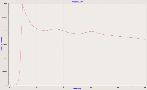
Figure 2: Typical long term behavior of a population with two distinct regimes. The first stage (from $n=0$ to $n$ around $10$–$20$) is the transient stage and the second stage is the stationary stage. Parameters values: $b=0$; $d=0.75$; $Z_{0}^{8}=1$; $R=10$; $N=100$; $K=10^{6}$; fitness distribution: Delta.

In the phenotypic model the transient regime corresponds to the beginning of the time evolution of the process. It is characterized, as noted before, by an instability of the relative frequencies of the replicative classes, an exponential growth of the progeny size, a decrease of the average reproduction rate, and an increase of both the phenotypic diversity and the phenotypic entropy.

The expected time (as function of the number of generations) of the relaxation to- wards an equilibrium after the bottleneck event, called recovery time (see the initial segment of the time series in Figure 3).

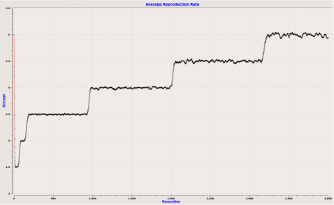
Figure 3: Average reproduction rate $=$ Relative growth rate. The “jumps” associated with the recovery time have heights about $0.5$. Parameters values: $b=0.000001$; $d=0.50$; $Z_{0}^{5}=1$; $R=10$; $N=4,000$; $K=10^{6}$; fitness distribution: Delta.

Let us assume, as usual, that the beneficial probability $b\approx 0$ and the founding population has $r_{\!*}(0)<R$. Then one observes that the progeny size, the average reproduction rate, the phenotypic diversity and phenotypic diversity display a time series with several plateaus. The “length” of each plateau is the number of generations that the population remains with the same value of $r_{\!*}(n)$ and the higher the plateau the longer, on average, is its length. The presence of a jump indicates that a progeny particle form a parental particle in the replicative class $r_{\!*}(n)$ has undergone a beneficial effect, that is, the active maximum replicative capability increases by $1$ unit: $r_{\!*}(n+1)=r_{\!*}(n)+1$. The occurrence of jumps can go on until $r_{\!*}(n)=R$. Therefore, the “length” of each plateau represents the time, in number of generations, required for a beneficial effect to occur on a particle at the highest replicative class and be retained in the population. The probability $\mathbf{P}\big{(}\text{jump in }r_{\!*}(n)\big{)}$ of occurrence of a jump event, when $r_{\!*}(n)<R$, may be estimated using equation (22) of Appendix B as

$$\mathbf{P}\big{(}\text{jump in }r_{\!*}(n)\big{)}\approx b\,u_{r_{\!*}(n)}\approx b\,(1-d)^{r_{\!*}(n)}$$

where $u_{r_{\!*}(n)}$ is the proportion of particles in the $r_{\!*}(n)$-th replicative class at generation $n$, which is the instantaneous maximum replicative capability at time $n$. Notice that, as $r_{\!*}(n)$ increases, $u_{r_{\!*}(n)}$ decreases monotonically and therefore, $\mathbf{P}\big{(}\text{jump in }r_{\!*}(n)\big{)}\to 0$ when $r_{\!*}(n)\to\infty$. This result highlights the asymmetry between the contributions of the beneficial probability versus the deleterious probability to the recovery time.

The “height” of a jump in the average reproduction rate time series is independent of the plateau where the jump occurs. In order to estimate the “height”, consider two consecutive levels on the time series of the average reproduction rate, the first “height” $\mu(n_{1})$ measured at generation $n_{1}$ and the second “height” $\mu(n_{2})$ measured at generation $n_{2}$, with $n_{1}<n_{2}$ not necessarily consecutive, such that $r_{\!*}(n_{2})=r_{\!*}(n_{1})+1$ and $\mu$ is approximately constant around $n_{1}$ and $n_{2}$. Thus, the difference $\mu(n_{2})-\mu(n_{1})$ gives an estimate of the height of the jump between two consecutive plateaus. When $b\approx 0$, equation (20) of Appendix B implies that $\mu(n)\approx r_{\!*}(n)(1-d)$ and hence

$$\mu(n_{2})-\mu(n_{1})\approx\big{(}r_{\!*}(n_{2})-r_{\!*}(n_{1})\big{)}(1-d)\approx 1-d\,.$$

For instance, in Figure 3 it can be readily seen that the height of the jumps is about $0.5$ and, in fact, $d=0.50$, $b=0.000001$ and hence $1-d=0.4999999$.

3.1.2 Stationary Regime

The advanced stage of the infection, also called chronic infection phase FWR03 ; MBTGH10 , is comprised by the stationary regime where the viral population has recovered its phenotypic (and genotypic) diversity and becomes better adapted to the new host environment by exhibiting rather stable relative frequencies of almost all variants.

In the phenotypic model the stationary regime corresponds to the asymptotic behavior of a super-critical branching process ($\mu>1$). But, as mentioned before, a surviving population described by super-critical branching process is never stationary (in the strict sense) and therefore this correspondence is not straightforward.

The normalized process $\bm{W}_{n}=\bm{Z}_{n}/\mu^{n}$ is stationary and, when $n\to\infty$, the random variable $Z^{r}_{n}/|\bm{Z}_{n}|$ converges to the asymptotic relative frequency $u_{r}$ of $r$-th replicative class. Consequently, the average reproduction rate $\langle\varrho(n)\rangle=\mu(n)$, the phenotypic diversity $\sigma^{2}_{\varrho}(n)$ and the phenotypic entropy $h_{\varrho}(n)$ remain essentially constant in time. Moreover, the maximum population size cut off $K$ ensures that the total progeny size remains constant in time with expected value $\langle|\bm{Z}_{n}|\rangle\approx\mu(n)\,K$.

During the stationary regime, the stability of the relative frequency of each class is maintained by a steady “flow of particles” from a replicative class to its adjacent classes, due to the deleterious probability $d$ and the beneficial probability $b$. The probability $c$ contributes maintenance of a constant proportion of particles in each replicative class. When the beneficial probability $b\neq 0$ the asymptotic distribution of classes $u_{r}$ is independent of the configuration of the founding population and, when $n$ is large enough, $r_{\!*}(n)=R$.

More importantly, when $b\approx 0$, the replicative classes that are most representative in the population are the classes near the mode of the distribution of classes $u_{r}$, also known as “most probable replicative capability”. The mode of $u_{r}=\mathrm{binom}(r;R,1-d)$ is given by $m(u_{r})=\lfloor(R+1)(1-d)\rfloor$, except when $(R+1)(1-d)$ happens to be an integer, then the two replicative classes corresponding to $(R+1)(1-d)-1$ and $(R+1)(1-d)$ are equally “most probable” (see F68 , here, $\lfloor x\rfloor$ denotes the greatest integer less than $x$). When $(1-d)\approx 1/2$ the mode is close to the average reproduction rate $\mu(n)=\langle\varrho(n)\rangle$ (see Figure 4).

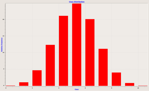
Figure 4: Histogram of the replicative classes. Parameter values: $b=0.000001$; $d=0.50$; $Z_{0}^{5}=1$; $R=10$; $N=4,000$; $K=10^{6}$; fitness distribution: Delta.

3.1.3 Threshold of Extinction

The threshold of extinction takes place when the deleterious rate is sufficiently high that it prevents the viral population of reaching the stationary regime but not high enough to induce the extinction of the population in the short run. Therefore, any small increase in the deleterious rate can push the population toward extinction, while any small decrement can allow the population to reach the stationary regime.

In the phenotypic model, the threshold of extinction corresponds to a critical branching process ($\mu=1$) and is characterized by instability of the relative frequencies of the replicative classes, the average replicative rate and the phenotypic diversity. The instability observed represents the impossibility of the viral population to preserve, due to the deleterious effects, particles with high replicative capability. The occurrence of an eventual extinction of the population is almost certain, although the time of occurrence of the extinction may be arbitrarily long if the initial population is sufficiently large. In other words, the threshold of extinction looks like an infinite transient phase and is the borderline between the stationary regime, where the transient phase ends at an stationary equilibrium, and the extinction in finite time.

Setting the parameters of the phenotypic model in order to obtain a critical branching process is a matter of “fine tuning”, since it requires that the probabilities $d$, $b$ and the maximum replicative capability $R$ satisfy the algebraic equation $\mu(b,d;R)=1$ – which is a non-generic condition (see Figure 5).

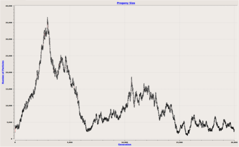
Figure 5: Progeny size of a population at the extinction threshold. Parameter values: $b=0$; $d=0.50$; $Z_{0}^{2}=1,000$; $R=2$; $N=20,000$; $K=10^{6}$; fitness distribution: Delta.

When $b=0$, the critical deleterious probability is $d_{c}=1-1/R$, for each fixed $R$. When $b\neq 0$ one may consider, for fixed $R$, the corresponding critical probability $d_{c}(b)$ as given implicitly by the equation $\mu(b,d_{c}(b),R)=1$ and the condition $\mu(0,d_{c}(0),R)=1$, with $d_{c}(0)=1-1/R$ (see Figure 10 of Appendix B). Since $b$ and $d$ are constrained to satisfy $b+d\leqslant 1$, there is a maximum value of $b$ such that $b+d_{c}(b)=1$, for each fixed $R$. Denote this maximum value by $b^{\star}(R)$. The number $b^{\star}(R)$ is the maximum beneficial probability such that the phenotypic model has three distinct regimes. In other words, if $b>b^{\star}(R)$ then $d<d_{c}(b)$ and the process never becomes extinct. In the parameter space of the phenotypic model, the critical probabilities $d_{c}(b^{\star})$ at $b^{\star}$ are given as the intersection of the boundary line $b+d=1$ with the critical curves $\mu(d,b,R)=1$ for each fixed $R$.

Using the expressions for the malthusian parameter obtained in ABCJ13a , it is easy to show that the following approximations hold (when $R\to\infty$)

$$\begin{split}b^{\star}(R)&\approx\dfrac{1}{R}-\dfrac{1}{R}\,\dfrac{(R-1)^{2}}{1+(R-1)^{2}}\\ d_{c}(b^{\star}(R))&\approx d_{c}(0)+\dfrac{1}{R}\,\dfrac{(R-1)^{2}}{1+(R-1)^{2}}\,.\end{split}$$ (1)

Here, one uses that $b^{\star}+d_{c}(b^{\star})=1$ and $d_{c}(0)=1-1/R$. Comparison of critical deleterious probability given by equations (1) with the correct values obtained by numerical computation using the mean matrix, shown in Table 2, indicate that the asymptotic expressions converge to the real values when $R\to\infty$.

$R$	$d_{c}(0)$	$d_{c}(b^{\star})$	$\tilde{d}_{c}(b^{\star})$	$|d_{c}(b^{\star})-\tilde{d}_{c}(b^{\star})|$
2	0.50	0.707	0.750	0.043
3	0.66	0.895	0.933	0.038
4	0.75	0.951	0.975	0.024
5	0.80	0.972	0.988	0.016
6	0.83	0.982	0.993	0.011

Table 2: Critical deleterious probabilities $d_{c}(0)$ and $d_{c}(b^{\star})$. The real values of $d_{c}(b^{\star})$ were obtained by numerical computation using the mean matrix and the values denoted by $\tilde{d}_{c}(b^{\star})$ were obtained using equations (1).

3.1.4 Extinction by Lethal Mutagenesis

The process of extinction of the viral population induced by increase of the deleterious rate is called lethal mutagenesis BSW07 . In the phenotypic model, the lethal mutagenesis corresponds to a sub-critical branching process ($\mu<1$). It is characterized by continuous decrease of the average replicative rate and by increase of the phenotypic diversity followed by a sudden decrease in the subsequent generations.

The progeny size and the phenotypic diversity increase during the first generations because the founding population still has reasonable replicative capability. However, increasing the size of the founding population does not prevent extinction, it only increases the time required for the extinction to occur. Increasing the deleterious probability $d$ decreases the time required for extinction and increasing beneficial probability $b$ can prevent extinction.

Note that when $b=0$ the population cannot achieve a replicative capability higher than the one present in the founding population. In this case, a population transmitted to a new host organism via a bottleneck event will have maximum replicative capability less or equal to the maximum replicative capability of the original population.

Interesting enough, there is a signature of the extinction process which may be directly observed in the behavior of the average reproduction rate curve $\mu(n)$. It is marked by an explosive growth in the variation of $\mu(n)$ as $n$ approaches the extinction time $n^{*}$ (see Figure 6).

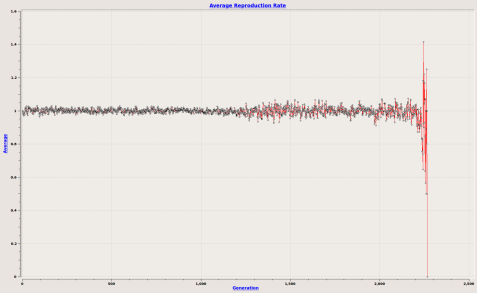
Figure 6: Lethal mutagenesis and the path to extinction. Parameter values: $b=0$; $d=0.501$; $R=2$; $N=2,500$; $K=10^{6}$; $\bm{Z}_{0}=(1000,2000,1000)$; fitness distribution: Delta.

The phenomenon of explosive growth near the extinction event may be detected by the oscillation of $\mu(n)$ in an interval ending at the last non-zero generation:

$$\mathrm{osc}(\mu)=\max_{n<n^{*}}\mu(n)\;-\min_{n<n^{*}}\mu(n)\,.$$

Even when the process is slightly super-critical, it is expected that the oscillation of $\mu(n)$ remains very small, with $\mathrm{osc}(\mu)\sim 10^{-3}$ for all $n$. On the other hand, when a slightly sub-critical process is approaching the extinction time $n^{*}$ one typically observes $\mathrm{osc}(\mu)\sim 10^{-1}$.

The expected time to extinction $\langle T_{\mathrm{ext}}\rangle$ of a branching process was determined in JKS07 : if $\mu\leqslant 1$ then

$$\langle T_{\mathrm{ext}}\rangle=\dfrac{\ln Z_{0}^{r_{\!*}}+\kappa}{-\ln\mu}$$

where $\kappa>0$ depends only on the parameters of the model (not on the initial population). It is easy to show that at the critical value of the malthusian parameter ($\mu=1$) equilibrium is never reached. A scaling exponent characterizing the behavior of expected time to extinction in a neighborhood of the critical value of the malthusian parameter can be obtained by considering the first order expansion of $\langle T_{\mathrm{ext}}\rangle$ about $1$:

$$\langle T_{\mathrm{ext}}\rangle\approx|\mu-1|^{-1}\,.$$

When $b=0$ one may write $\langle T_{\mathrm{ext}}\rangle$ as a function of the deleterious probability and the critical deleterious probability $d_{c}=1-1/R$ as

$$\langle T_{\mathrm{ext}}\rangle\approx\frac{1}{R}|d-d_{c}|^{-1}$$

since $|\mu-1|=R|d-d_{c}|$. This “scaling law” is formally identical to the one obtained in GD15 for the error threshold of the deterministic quasispecies model as a function of the mutation rate.

3.2 Populational Variance and the Role of Fitness Distributions

All properties of the phenotypic model that have been discussed so far are related to the mean matrix of the model, that is, they depend only on the first moments of the branching process and may be called “first order properties”. In particular, they are independent of the choice of the family of fitness distributions. If we want to see how the fitness distributions influence the evolution of the population we must to look at a “second order property”, which is expected to depend on the second moments of the fitness distributions (see Table 1).

Distribution	$\sigma^{2}_{r}$	$\phi$
Deterministic	$0$	$0$
Poisson	$r$	$\langle\varrho\rangle$
Geometric	$r(r+1)$	$\langle\varrho\rangle\big{(}\langle\varrho\rangle+1\big{)}+\sigma^{2}_{\varrho}$
$\tfrac{1}{2}$-Binomial	$r/2$	$\langle\varrho\rangle/2$
Power law	$+\infty$	$+\infty$

Table 3: Location-scale families of fitness distribution of the ENVELOPE program, their variance and the corresponding normalized populational variances.

The simplest property of second order is given by the population variance $\sigma^{2}$ associated with the malthusian parameter $\mu$ (namely, the relative growth rate). Furthermore, the difference between the populational variance and the (squared) phenotypic diversity, called normalized populational variance and denoted by $\phi$ is a very interesting quantity to be measured, since it satisfies

$$\phi=\sigma^{2}-\sigma^{2}_{\varrho}=\sum_{r=0}^{R}\sigma^{2}_{r}\,u_{r}$$ (2)

In other words, $\phi$ is a weighted average of the variances $\sigma^{2}_{r}$ of the fitness distributions. See Appendix A for the precise definition of $\sigma^{2}$ and the proof of the second equality in equation (2).

Given a location-scale family of fitness distributions $t_{r}$ such that $\sigma_{r}^{2}$ is at most a quadratic polynomial on $r$, eqaution (2) allows one to write the corresponding normalized population variance $\phi$ in terms of the average reproduction rate $\langle\varrho\rangle$ and the phenotypic diversity $\sigma_{\varrho}^{2}$. Hence, $\phi$ can be exactly computed for all location-scale families of distributions used in the ENVELOPE program (see Table 3).

It is important to stress that unlike the malthusian parameter, the normalized populational variance does depend on the choice of the family of fitness distributions. Recall that the malthusian parameter depends only on the mean matrix, which depends on the fitness distributions $t_{r}$ only through its expectation values. Since we have imposed the same normalization condition that the expectation value of $t_{r}$ is $r$ for all families of fitness distributions, it follows that the mean matrix, and hence the malthusian parameter, does not depend on the family of fitness distributions. On the other hand, the variances of different families of fitness distributions are not necessarily the same. For instance, if $t_{r}$ is the family of Poisson distributions then $\sigma^{2}_{r}=r$ and thus $\phi=\mu$.

Assume that $b=0$ (then $c=1-d$). From the expression of the asymptotic distribution of classes (21) one obtains: $\langle\varrho\rangle=\mu=R(1-d)$ and $\sigma_{\varrho}^{2}=Rd(1-d)$. Moreover, when $b\neq 0$ is sufficiently small, formula 22 ensures that $\langle\varrho\rangle$ and $\sigma_{\varrho}^{2}$ are approximated by the corresponding values for $b=0$ and the same holds for $\phi$.

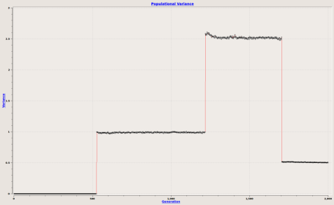
Figure 7: Normalized population variance $\phi$, with $\langle\varrho\rangle=1$ and $\sigma^{2}_{\varrho}=0.5$. Parameter values: $b=0$; $d=0.50$; $R=2$; $N=2,000$; $K=10^{6}$; $Z_{0}^{2}=10,000$; fitness distributions: Delta ($\phi=0$), Poisson ($\phi=1$), Geometric ($\phi=2.5$), Binomial ($\phi=0.5$).

For instance, in Figure 7 we show the graph of the normalized population variance $\phi(n)$, at generation $n$, from a simulation in which we switched among the four families of fitness distributions with finite variance using the “Video” function of the ENVELOPE program to pause the simulation and change the type of fitness distribution.

Finally, it is worth to remark that the impact of the power law family of fitness distribution on the evolution of the population is very distinct from the other families, because, unlike the other fitness distributions, it has infinite variance. One of the consequences of this property is the appearance of intense bursts of progeny production clearly seen on the times series of progeny size and the average reproduction rate (see Figure 8). The instability caused by unbounded fluctuations coupled with the finite population size effect (even for large $K$) is responsible for the generation of a train of sparse and intense bursts of progeny production. On the other hand, this instability coupled with finiteness effect may also provoke sudden drops on the progeny size driving the population to a premature extinction, even if the malthusian parameter is above $1$. Because of these extreme phenomena one would be led to believe that the phenotypic model with the power law family of fitness distributions is an exception to the general result: any property derived from the mean matrix is independent of the fitness distribution. It is not the case. In fact, if one considers the time-average of any quantity that is time-dependent over a time interval $[n_{0},N]$ during the stationary regime, let’s say

$$\bar{\mu}(N)=\frac{1}{N}\sum_{n=n_{0}}^{N}\mu(n)\,,$$

then it is expected that $\bar{\mu}(N)$ becomes very close to the asymptotic value of the relative growth rate $\mu$ when $N$ is sufficiently large.

For instance, in Figure 8 the time-average of the progeny size $\bar{\mu}(N)$ is around $14,000$, while the expected progeny size for the model is $\mu K=R(1-d)K=2\times 0.7\times 10^{4}=1.4\times 10^{4}=14,000$, in full agreement with the general theory.

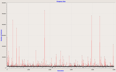
Figure 8: Power law induced bursts (viral blips), with time-average progeny size around $14,000$ viral particles, going up to $400,000$ - $500,000$ particles during an intense burst. Parameter values: $b=0$; $d=0.30$; $R=2$; $N=5,000$; $K=10^{4}$; $Z_{0}^{2}=10,000$; fitness distribution: Power law.

3.3 Finite Population Size and Mutational Meltdown

Recently, Matuszewski et al. MOBJ17 reviewed the literature about theories and models describing the extinction of populations owing to the excessive accumulation of deleterious mutations or effects and distinguished two apparently distinct lines of research, represented by the lethal mutagenesis models BSW07 and the mutational meltdown models LG90 which, nonetheless, display a considerable amount of similarity.

Indeed, as shown in BSW07 ; ABCJ13b ; ABCJ13a , lethal mutagenesis is independent of population size, hence it is fundamentally a deterministic process that operates even on very large populations. Although the outcome of lethal mutagenesis is deterministic, other aspects of the population dynamics (such as extinction time, individual trajectories of progeny size, etc.) are not. On the other hand, the mutational meltdown generally works within the context of “small” population sizes in which stochastic effects caused by random drift play an important role.

We believe that the approach presented here may help shed some light on this issue. There is one ingredient in the mutational meltdown theory that is absent in the lethal mutagenesis theory: the carrying capacity. This is true even for models with finite population, such as DSS85 and the phenotypic model, in their theoretical formulations as branching process. However, as seen before, the computational implementation of the phenotypic model required the introduction a cut off $K$ in order to bound the growth of the population. If the cut off is taken as basic constituent of the phenotypic model, and not merely a convenient device, then it can play a role similar to a carrying capacity and the model may no longer be considered a “pure” branching process, but a self-regulating branching process MS12 ; MSR13 .

In a self-regulating branching process not all the offspring produced in a given generation will to produce offspring in the next generation and hence, it is necessary to introduce a survival probability distribution $S(n|T_{n})$, to stochastically regulate the survival of offspring at any generation $n$ as a function of the total population size $T_{n}=|\bm{Z}_{n}|$. The motivation behind this definition is the following: if the population size at a generation $n$ exceeds the carrying capacity of the environment then, due to competition for resources, it is less likely that an offspring produced in that generation will survive to produce offspring at generation $n+1$.

Let $S(n|T_{n})$ denote the conditional probability that any offspring produced at generation $n$ survives to produce offspring at generation $n+1$, given that the population has $T_{n}$ individuals at generation $n$. If we define the conditional probability $S$ as

$$S(n|T_{n})=\left\{\begin{array}[]{l@{\quad\text{if}\quad}l}K/T_{n}&T_{n}>K\\ 1&T_{n}\leqslant K\end{array}\right.$$

then the phenotypic model becomes a self-regulating process with carrying capacity $K$. Moreover, when $K\to\infty$ the self-regulating process reduces to a “pure” branching process.

If $K$ is not large enough then a kind of random drift effect due to finite population size may take place, which happens when the fittest replicative classes are lost by pure chance, since its frequency is typically very low (they are the lesser represented replicative class in the population). If the loss of the fittest replicative class occurs a sufficient number of times then the population will undergo extinction. Note that this may happen even when the process is super-critical, namely, it is far from the extinction threshold. This is not a contradiction with the definition of extinction probability, since a super-critical process still has a positive probability to become extinct (see Appendix A).

Now suppose that $b=0$, the initial population has active maximum replicative capability $r_{\!*}(0)$ and the carrying capacity $K$ is sufficiently small (we shall give an estimate of $K$ in a moment). Then, as mentioned before, the value $r_{\!*}=r_{\!*}(0)$ acts as the maximum replicative capability for that population. Moreover, if the highest replicative class $r_{\!*}$ is lost by chance, that is, if $r_{\!*}(n+1)=r_{\!*}(n)-1$, then it can not be recovered anymore and hence, from that time on the maximum replicative capability for that population has dropped by $1$ unit. This may be seen as a manifestation of the “Muller’s ratchet”, since the population has accumulated a deleterious effect in an irreversible manner.

For sake of concreteness, let us assume that $r_{\!*}=R$ and $d$ are such that $(R-1)(1-d)<1$, but $R(1-d)>1$. Then, at the beginning of the process, the malthusian parameter is $\mu=R(1-d)>1$ and the process is super-critical. However, if at some generation $n$, the $R$-th replicative class is lost by chance, then $R$ drops by $1$ and $\mu=(R-1)(1-d)<1$, so the process becomes sub-critical and the population becomes extinct very quickly. In this case, the frequency of the $R$-th replicative class is $(1-d)^{R}$ and fraction of particles that are purged, at each generation, is $R(1-d)-1$, hence the fraction of particles that are left in the $R$-th replicative class, at each generation, is $\nu_{R}=2(1-d)^{R}-R(1-d)^{R+1}$. If $K\approx 1/\nu_{R}$ then there will be, on average, $1$ particle of class $R$ per generation – it is very unlikely that this replicative class will be retained for a long period of time. Therefore, in order to avoid the random drift effect $K$ should be at least of the order of $10\times R(1-d)/\nu_{R}$, or higher. At each “click of the ratchet” the fittest replicative class is lost and there is a drop in the malthusian parameter by $(1-d)$, until $r_{\!*}(1-d)$ becomes less than $1$, where $r_{\!*}$ is the maximum replicative capability at the current generation. This drop occurs in the phenotypic diversity and the phenotypic entropy, as well (see Figure 9).

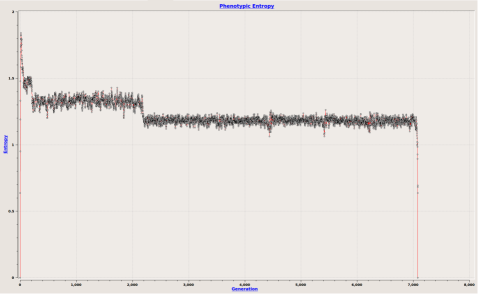
Figure 9: Extinction by mutational meltdown. Phenotypic Entropy time series. At the beginning the branching process is super-critical with $\mu=3.41$. Parameter values: $b=0$; $d=0.659$; $R=10$; $N=10,000$; $K=2,000$; $Z_{0}^{10}=6,000$; fitness distributions: Delta.

If one writes the usual condition for occurrence of extinction $r_{\!*}(1-d)<1$ as

$$(1-d)<1/r_{\!*}$$

then this is an exact phenotypic analogue of the mutational meltdown extinction criterion. Indeed, $r_{\!*}$ is the phenotypic analogue of absolute growth rate of the population at time $n$ and $c=(1-d)$, the probability of occurrence of a neutral fitness effect per individual particle, is the phenotypic analogue of the mean viability (compare with the equations in LBBG93 ; LG90 ).

4 Conclusion and Outlook

In this paper we have exhaustively explored a model for the evolution of RNA virus, which was formulated as a multivariate branching process, called phenotypic model. The theory of branching processes provides a suitable framework endowed with concepts and analytic tools allowing for the investigation of evolutionary aspects of RNA viruses propagating along different adaptive landscapes.

One of the greatest virtues of the phenotypic model is its simplicity. Since the model has essentially only $3$ parameters it is possible to analytically compute the spectrum of its mean matrix and, applying the classification of multitype branching processes, obtain a complete qualitative description its “generic behaviors”, that is, the most likely outcomes of the model’s asymptotic dynamics.

The maximum replication capacity $R$ and the probabilities of occurrence of deleterious effects $d$ entirely determine whether a viral population becomes extinct infinite time or not. On the other hand, the third parameter, the probability of occurrence of beneficial effects $b$, plays a distinct role from the other two probabilities, functioning as a threshold parameter which determines if the model posses the three typical regimes of a branching process or just one regime (super-critical).

The model provides several statistical measures, such as average growth rate, phenotypic diversity, phenotypic entropy and population variance, that allows one to asses the stochastic dynamics of a viral population. The dynamics of the associated deterministic quasispecies model is given by a mean field limit where the mean matrix completely determines the dynamics (see Appendix C). Hence it is possible to establish a relation between statistical measures mentioned above and the fundamental macroscopic parameters that characterize the evolutionary dynamics of a quasispecies. In particular, the models of SS82 ; SS1988 could be used as a representation of the evolution of mean values obtained from the mean matrix of a branching process. By extending the scope of the model to age dependent branching processes AN72 could allow the incorporation other statistical measures, such as evolutionary entropy D05 ; D2013 . This quantity could provide a more precise understanding of viral diversity given the fact that population sizes of viral population are finite.

Despite its conceptual appeal, the phenotypic model has some important drawbacks. The first limitation is the lack of feedback from the host organism on the virus population, since the probabilities of fitness effects are independent of time. This shortcoming is partially handled in the ENVELOPE program by the “Video” function, which allows one to pause the simulation and change the probabilities and emulate the host’s “response” against the virus. The second limitation is the lack of the phenotype-to-genotype map, i.e, the relationship between genotypic and phenotypic change. The motivation to use a phenotypic approach was to avoid the severe difficulties in modeling this kind of mapping A91 ; FZOW17 .

Even though there is no phenotype-to-genotype map, it still is possible to draw some consequences about mutation rates from a purely phenotypic model ABCJ13b . For example, under the assumption that the mutation rate $U$ is sufficiently high (between $0.1$ and $1$), the probability that a spontaneous mutation produces a deleterious effect may be estimated as follows: if we assume that the number of mutations in a genome follows a Poisson distribution, then $d_{\mathrm{sp}}\approx 1-\mathrm{e}^{-f_{d}}$, where $f_{d}$ is the probability that a spontaneous mutation has a deleterious effect KM66 . Values of $f_{d}$ have been measured in vitro for a few viruses and are shown in Table 4, along with the respective mutation rates $U$. Now, $d_{\mathrm{sp}}$ provides a lower bound for the deleterious probability and since the value $d_{\mathrm{sp}}\approx 1/2$ seems to be typical for RNA viruses, the interval $1/2<d<d_{c}=1-1/R$ is more likely to be the range of the parameter $d$. Moreover, it is easy to see that the phenotypic diversity and the phenotypic entropy are maximal when $d$ is near $1/2$, for any value of $R$ ABCJ13b . One could speculate that this is a universal property for RNA viruses that replicate under high mutational rates associated with a maximization principle that seeks to improve the chances of survival D12 .

Virus	Group	$f_{d}$	$d_{\mathrm{sp}}$	$U$	REFS.
VSV	($-$)ssRNA (V)	$0.69$	$0.50$	$0.1$	SME04 ; FMS05
Q$\beta$	($+$)ssRNA (IV)	$0.74$	$0.52$	$0.6$	CCS09 ; BCDS13
TEV	($+$)ssRNA (IV)	$0.77$	$0.53$	$0.5$	CIE07 ; TE10
$\Phi$6	dsRNA (III)	$0.42$	$0.34$	$0.03$	BC04 ; BGSS07
$\Phi$X174	ssDNA (II)	$0.77$	$0.53$	$0.003$	CCS09 ; CDS09
F$1$	ssDNA (II)	$0.65$	$0.47$	$0.004$	PDC10 ; D12

Table 4: Measured values of $f_{d}$, the corresponding deleterious probability $d_{\mathrm{sp}}=1-\mathrm{e}^{-f_{d}}$ and genome-wide spontaneous mutation rate $U$.

The first main result of this paper is concerns the role of the fitness distributions. The fitness distributions of the phenotypic model were motivated by the results and observations of ZYY09 on the distribution of single cell progeny sizes of RNA viruses. In ZYY09 the authors demonstrated that even in a well controlled experiment, using the same viral isolate, same infection parameters and clonally expanded target cells, progeny sizes can vary substantially. The variance on progeny sizes in such uniform environment indicates that RNA viruses replication bears in some way a portion of unpredictability. In this manner, it is impossible to know how many particles will be produced by a cell until the infection takes place and the progeny is released. Thus, fitness distributions provide a simple way to accommodate this unpredictability into each viral replication cycle. In fact, as shown here, some types of fitness distributions may have a substantial impact on the evolution of the viral population, most notably the power law. The extreme behavior produced by the power law resembles that of the “viral load blips” frequently observed in HIV patients under highly active antiretroviral therapy (HAART) DML03 ; NKK05 ; NK06 ; LKSN06 ; G07 ; RP09a ; RP09b , with undetectable or very low viral loads. This particular prediction of the model agrees with the assumption that these events are simply due to random fluctuation of the replication process, since after a “blip” the viral load quickly returns to its basal values.

The second main result of this paper is concerned with the mechanisms that drive a RNA virus population to extinction. As mentioned before, in the framework of multitype branching processes, there are essentially to main attributes associated with this type of event: the probability of occurrence of deleterious effects $d$ and the maximum replicative capability $R$. If in addition to these two, one also considers the carrying capacity as a fundamental parameter of the phenotypic model then it is possible to show that the two principal mechanisms of extinction, lethal mutagenesis and mutational meltdown, are based on the same mathematical principle. Therefore, as far as the phenotypic model is concerned, this is a proof of the claim MOBJ17 that these two mechanisms are “two sides of the same coin”.

Finally, for the sake of simplicity the phenotypic model considers only three basic types of fitness effects; the deleterious, beneficial and neutral. However, fitness effects represent a broad group forces acting on virus replication and one possible direction for further investigation would be to ungroup some of these forces and test their action. For example, on the deleterious side, the inclusion of defective interfering particles could yield another extinction mechanism, whereas on the beneficial side, the inclusion of recombination could help the viral population escape from extinction.

Acknowledgments.

LG acknowledges the support of FAPESP through the grant number 14/13382-1. BG and DC received financial support from CAPES.

Software Availability and Requirements.

The ENVELOPE program was written in C++ programming language, using the Qt 4.8.6 framework, with the Qwt 5.2.1 library. It runs on Linux and MAC-OSX operating systems and requires at least 2 GB of RAM memory and 1.5 MB of disk space. Its distribution is free to all users under the LGPL license. Binary files for Linux and MAC-OSX operating systems are available for download at: https://envelopeviral.000webhostapp.com

Author contribution:

LG and DC contributed equally to this work. LMRJ and FA contributed equally to this work. Conceived the model and formulated the underlying theory: LMJR and FA. Implemented the software: LG, DC and BG. Simulated the model and analyzed the output: LG and DC. Wrote the paper: LMRJ and FA.

Appendices

Appendix A Review of Multitype Branching Process Theory

A discrete-time multitype branching process with types or classes indexed by a non-negative integer $r$ ranging from $0$ to $R$ is described by a sequence of vector-valued random variables $\bm{Z}_{n}=(Z_{n}^{0},\ldots,Z_{n}^{R})$, ($n=0,1,\ldots$), where $Z_{n}^{r}$ is the number of particles of type or class $r$ in the $n$-th generation. The initial population is represented by a vector of non-negative integers $\bm{Z}_{0}$ (also called a multi-index) which is non-zero and non-random. The time evolution of the population is determined by a vector-valued discrete probability distribution $\bm{\zeta}(\bm{i})=\big{(}\zeta_{r}(\bm{i})\big{)}$, defined on the set of multi-indices $\bm{i}=(i^{0},\ldots,i^{R})$, called the offspring distribution of the process, which is usually encoded as the coefficients of a vector-valued multivariate power series $\bm{f}(\bm{z})=\big{(}f_{r}(\bm{z})\big{)}$, called probability generating function (PGF).

The mean matrix or the matrix of first moments $\bm{M}=\{M_{ij}\}$ of a multitype branching process describes how the average number of particles in each type or class evolves in time and is defined by $M_{ij}=\mathbf{E}(Z_{1}^{i}|Z^{j}_{0}=1)$, where $Z^{j}_{0}=1$ is the abbreviation of $\bm{Z}_{0}=(0,\ldots,1,\ldots,1)$. In terms of the probability generating function $\bm{f}=(f_{0},\ldots,f_{R})$ it is given by

$$M_{ij}=\dfrac{\partial f_{j}}{\partial z_{i}}(\bm{s})\bigg{|}_{\bm{s}=\bm{1}}$$ (3)

where $\bm{1}=(1,1,\ldots,1)$. Typically, the mean matrix $\bm{M}$ is non-negative and hence it has a largest non-negative eigenvalue. When the largest eigenvalue is positive, it coincides with the spectral radius of $\bm{M}$ and it is called, following Kimmel and Axelrod K02 , the malthusian parameter $\mu$.

The vector of extinction probabilities of a multitype branching process, denoted by $\bm{\gamma}=(\gamma_{0},\ldots,\gamma_{R})$, where $0\leqslant\gamma_{r}\leqslant 1$, is defined by the condition that $\gamma_{r}$ is the probability that the process eventually become extinct given that initially there was exactly one particle of class $r$.

The classification theorem of multitype branching proceses states that there are only three possible regimes for a multitype branching process H63 ; AN72 ; K02 :

Super-critical:

If $\mu>1$ then $0\leqslant\gamma_{r}<1$ for all $r$ and, with positive probability the population survives indefinitely.

Sub-critical:

If $\mu<1$ then $\gamma_{r}=1$ for all $r$ and with probability $1$ the population becomes extinct in finite time.

Critical:

If $\mu=1$ then $\gamma_{r}=1$ for all $r$ and with probability $1$ the population becomes extinct, however, the expected time to the extinction is infinite.

When a multitype branching process is super-critical it is expected that, according to the “Malthusian Law of Growth” it will grow indefinitely at a geometric rate proportional to $\mu^{n}$, where $\mu$ is the malthusian parameter, $\bm{Z}_{n}\approx\mu^{n}\,\bm{W}_{n}$ for some bounded random vector $\bm{W}_{n}$, when $n\to\infty$. The formalization of the above heuristic reasoning is given by the Kesten-Stigum limit theorem for super-critical multitype branching processes (see KS66a ; KS66b ; KS67 ). If $\bm{W}_{n}=\bm{Z}_{n}/\mu^{n}$ then there exists a scalar random variable $W\neq 0$ such that, with probability one,

$$\lim_{n\to\infty}\bm{W}_{n}=W\,\bm{u}$$ (4)

where $\bm{u}$ is the right eigenvector corresponding to the malthusian parameter $\mu$ and

$$\mathbf{E}(W|\bm{Z}_{0})=\bm{v}^{\mathrm{t}}\bm{Z}_{0}$$ (5)

where $\bm{v}$ is the left eigenvector corresponding to the malthusian parameter $\mu$. The vectors $\bm{u}$ and $\bm{v}$ may be normalized so that $\bm{v}^{\mathrm{t}}\bm{u}=1$ and $\bm{1}^{\mathrm{t}}\bm{u}=1$ where ^t denotes the transpose of a vector. Moreover, under the assumption that $\bm{M}$ is non-negative (which is satisfied by the phenotypic model (18)), the right and left eigenvectors corresponding to the malthusian parameter are non-negative.

The normalization of right eigenvector $\bm{u}=(u_{0},\ldots,u_{R})$ implies that $\sum_{r}u_{r}=1$ and therefore one has the “law of convergence of types” (see KLPP94 )

$$\lim_{n\to\infty}\dfrac{\bm{Z}_{n}}{|\bm{Z}_{n}|}=\bm{u}\,,$$ (6)

where $|\bm{Z}_{n}|=\sum_{r}Z_{n}^{r}$ is the total population at the $n$-th generation and the equality holds almost surely. Equation (6) asserts that the asymptotic proportion of a replicative class $r$ converges almost surely to the constant value $u_{r}$.

In particular, equation (6) implies that the malthusian parameter is the asymptotic relative growth rate of the population

$$\mu=\lim_{n\to\infty}\dfrac{|\bm{Z}_{n}|}{|\bm{Z}_{n-1}|}=\lim_{n\to\infty}\dfrac{1}{|\bm{Z}_{n-1}|}\,\sum_{j=1}^{|\bm{Z}_{n-1}|}\#[\,j\,]$$ (7)

since $|\bm{Z}_{n-1}|$ may be interpreted as the set of “parental particles” of the particles in the $n$-th generation and $|\bm{Z}_{n}|$ is the sum of the “progeny sizes” $\#[\,j\,]$ of the “parental particles” $j$ from the previous generation.

Now consider the quantitative random variable $\varrho$ defined on the set of classes $\{0,\ldots,R\}$ and having probability distribution $(u_{0},\ldots,u_{R})$, called the asymptotic distribution of classes. When the classes are indexed by their expectation values the variable $\varrho$ associates to a random particle its expected class

$$\mathbf{P}(\varrho=r)=u_{r}\,.$$

Therefore, one can define the average reproduction rate of the population as

$$\langle\varrho\rangle=\sum_{r=0}^{R}r\,u_{r}\,.$$ (8)

Using equations (4), (5), (6) one can show that the average reproduction rate is equal to the malthusian parameter:

$$\langle\varrho\rangle=\mu\,.$$ (9)

The average population size at the $n$-th generation is $|\langle\bm{Z}_{n}\rangle|=\sum_{r=0}^{R}\langle Z^{r}_{n}\rangle$. Then for $n\to\infty$, equation (4) gives $|\langle\bm{Z}_{n}\rangle|\approx\mu^{n}|\langle\bm{W}_{n}\rangle|\approx\mu^{n}\langle W\rangle$ and so

$$\mu=\lim_{n\to\infty}\dfrac{|\langle\bm{Z}_{n}\rangle|}{|\langle\bm{Z}_{n-1}\rangle|}$$ (10)

On the other hand, from the definition of mean matrix and its form (18), one has

$$|\langle\bm{Z}_{n}\rangle|=|\bm{M}\,\langle\bm{Z}_{n-1}\rangle|=\sum_{r=0}^{R}r\,\langle Z^{r}_{n-1}\rangle\,.$$

Now dividing by $|\langle\bm{Z}_{n-1}\rangle|$ and taking the limit $n\to\infty$ gives

$$\mu=\lim_{n\to\infty}\dfrac{|\langle\bm{Z}_{n}\rangle|}{|\langle\bm{Z}_{n-1}\rangle|}=\lim_{n\to\infty}\sum_{r=0}^{R}r\,\dfrac{\langle Z^{r}_{n-1}\rangle}{|\langle\bm{Z}_{n-1}\rangle|}=\sum_{r=0}^{R}r\,u_{r}=\langle\varrho\rangle$$

where here we used equations (5) and (6) in the third equality from left to right.

In analogy with the characterization of the malthusian parameter as given by equation (7), one may define the asymptotic populational variance

$$\sigma^{2}=\lim_{n\to\infty}\dfrac{1}{|\bm{Z}_{n-1}|}\,\sum_{j=1}^{|\bm{Z}_{n-1}|}\#[\,j\,]^{2}-\mu^{2}$$ (11)

and in analogy with the mean reproduction rate, one may define the (squared) phenotypic diversity as

$$\sigma_{\varrho}^{2}=\langle\varrho^{2}\rangle-\langle\varrho\rangle^{2}$$ (12)

By decomposing the sum in equation (11) according to the classes $r$, one obtains

$$\sum_{j=1}^{|\bm{Z}_{n-1}|}\#[\,j\,]^{2}=\sum_{r=0}^{R}\sum_{j_{r}=1}^{Z_{n-1}^{r}}\#[\,j_{r}\,]^{2}$$

where $j_{r}$ runs over the particles of class $r$ for $r=0,\ldots,R$ and $\#[\,j_{r}\,]$ are independent random variables assuming non-negative values with probability distribution $t_{r}$, called fitness distribution of class $r$.

Denoting the variance of the fitness distribution $t_{r}$ by $\sigma^{2}_{r}$, one may write the limit in equation (11) as

$$\begin{split}\sigma^{2}&=\lim_{n\to\infty}\dfrac{1}{|\bm{Z}_{n-1}|}\,\sum_{j=1}^{|\bm{Z}_{n-1}|}\#[\,j\,]^{2}-\mu^{2}\\ &=\lim_{n\to\infty}\dfrac{1}{|\bm{Z}_{n-1}|}\,\sum_{r=0}^{R}\left[Z^{r}_{n-1}\left(\dfrac{1}{Z^{r}_{n-1}}\sum_{j_{r}=1}^{Z_{n-1}^{r}}\#[\,j\,]^{2}-r^{2}\right)+Z^{r}_{n-1}\right]-\mu^{2}\\ &=\lim_{n\to\infty}\dfrac{1}{|\bm{Z}_{n-1}|}\,\sum_{r=0}^{R}(\sigma^{2}_{r}+r^{2})Z^{r}_{n-1}-\mu^{2}\end{split}$$

Then equations (6), (9) and (12) give

$$\sigma^{2}=\sum_{r=0}^{R}(\sigma^{2}_{r}+r^{2})\,u_{r}-\mu^{2}=\sum_{r=0}^{R}\sigma^{2}_{r}\,u_{r}+\sigma^{2}_{\varrho}$$ (13)

The difference between the asymptotic populational variance and the (squared) phenotypic diversity, called normalized populational variance, is the weighted average of the variances of the fitness distributions

$$\phi=\sigma^{2}-\sigma^{2}_{\varrho}=\sum_{r=0}^{R}\sigma^{2}_{r}\,u_{r}\,.$$ (14)

In particular, when the family of fitness distributions is the deterministic family the populational variance is exactly the phenotypic diversity (that is $\phi=0$). This is an expected result since the Delta distributions $t_{r}(k)=\delta_{rk}$ have zero variance and hence the only source of fluctuation of the population size is due to its stratification into replicative classes, which is expressed by the phenotypic diversity.

Appendix B Mathematical Basis of the Phenotypic Model

Based on the general aspects of the phenomenon of viral replication described before it is compelling to model it in terms of a branching process. At each replicative cycle, every parental particle in the replicative class $r$ produces a random number of progeny particles that is independently drawn from the corresponding fitness distribution.

A fitness distribution is a member of a location-scale family of discrete probability distributions $t_{r}$ parameterized by the replicative classes ($r=0,\ldots,R$) assuming non-negative integer values and normalized so that the expectation value of $t_{r}$, defined as $\sum_{k}k\,t_{r}(k)$, is exactly $r$ and $t_{0}(k)=\delta_{k0}$. Here $\delta_{kr}=1$ if $k=r$ and $\delta_{kr}=0$ if $k\neq r$. Therefore, each particle in the viral population is characterized by the mean value of its fitness distribution, called mean replicative capability. Viral particles with replicative capability equal to zero ($0$) do not generate progeny; viral particles with replicative capability one ($1$) generate one particle on average; viral particles with replicative capability two ($2$) generate two particles on average, and so on. Typical examples of location-scale families of discrete probability distributions that can be used as fitness distributions are:

1. The family of Deterministic (Delta) distributions: $t_{r}(k)=\delta_{kr}$.

2. The family of Poisson distributions: $t_{r}(k)=\mathrm{e}^{-r}\tfrac{r^{k}}{k!}$.

Note that in the first example, the replicative capability is completely concentrated on the mean value $r$ – that is, the particles have deterministic fitness. On the other hand, in the second example the fitness is truly stochastic.

During the replication, each progeny particle always undergoes one of the following effects:

Deleterious effect:

the mean replication capability of the respective progeny particle decreases by one. Note that when the particle has capability of replication equal to $0$ it will not produce any progeny at all.

Beneficial effect:

the replication capability of the respective progeny particle increases by one. If the mean replication capability of the parental particle is already the maximum allowed then the mean replication capability of the respective progeny particles will be the same as the replicative capability of the parental particle.

Neutral effect:

the mean replication capability of the respective progeny particle remains the same as the mean replication capability of the parental particle.

To define which effect will occur during a replication event, probabilities $d$, $b$ and $c$ are associated, respectively, to the occurrence of deleterious, beneficial and neutral effects. The only constraints these numbers should satisfy are $0\leqslant d,b,c\leqslant 1$ and $b+c+d=1$. In the case of in vitro experiments with homogeneous cell populations the probabilities $c$, $d$ and $b$ essentially refer to the occurrence of mutations.

The probability generating function (PGF) of the phenotypic model with $b=0$ and $t_{r}(k)=\delta_{kr}$ is (see Antoneli et al. ABCJ13b ; ABCJ13a for details):

$$\begin{split}f_{0}(z_{0},z_{1},\ldots,z_{R})&=1\\ f_{1}(z_{0},z_{1},\ldots,z_{R})&=dz_{0}+cz_{1}\\ f_{2}(z_{0},z_{1},\ldots,z_{R})&=(dz_{1}+cz_{2})^{2}\\ &\vdots\\ f_{R}(z_{0},z_{1},\ldots,z_{R})&=(dz_{R-1}+cz_{R})^{R}\end{split}$$ (15)

Note that the functions $f_{r}(z_{0},z_{1},\ldots,z_{R})$ are polynomials whose coefficients are exactly the probabilities of the binomial distribution $\mathrm{binom}(k;r,1-d)$. The PGF in the case with general beneficial effects and with a general family of fitness distribution (which reduces to the previous PGF when $b=0$ and $t_{r}(k)=\delta_{kr}$) is given by.

$$\begin{split}f_{0}(z_{0},z_{1},\ldots,z_{R})&=1\\ f_{1}(z_{0},z_{1},\ldots,z_{R})&=\sum_{k=0}^{\infty}\,t_{1}(k)\,(dz_{0}+cz_{1}+bz_{2})^{k}\\ f_{2}(z_{0},z_{1},\ldots,z_{R})&=\sum_{k=0}^{\infty}\,t_{2}(k)\,(dz_{1}+cz_{2}+bz_{3})^{k}\\ &\vdots\\ f_{R}(z_{0},z_{1},\ldots,z_{R})&=\sum_{k=0}^{\infty}\,t_{R}(k)\,(dz_{R-1}+(c+b)z_{R})^{k}\end{split}$$ (16)

Note that in the last equation the beneficial effect acts like the neutral effect. This is a kind of “consistency condition” ensuring that the populational replicative capability is, on average, upper bounded by $R$. Even though it is possible that a parental particle in the replicative classes $R$ eventually has more than $R$ progeny particles when $t_{r}$ is not deterministic, the average progeny size is always $R$.

Finally, it is easy to see that the PGF of the two-dimensional case of the phenotypic model with $b=0$ and $z_{0}=1$ (and ignoring $f_{0}$) reduces to

$$f(z)~{}=~{}\sum_{k=0}^{\infty}\,t(k)\,((1-c)+cz)^{k}~{}=~{}\sum_{k=0}^{\infty}\,t(k)\,(1-c(1-z))^{k}\,.$$ (17)

This is formally identical to the PFG of the single-type model proposed by (DSS85, , p. 255, eq. (49)) for the evolution of polynucleotides. In their formulation, $c=p^{\nu}$ is the probability that a given copy of a polynucleotide is exact, where the polymer has chain length of $\nu$ nucleotides and $p$ is the probability of copying a single nucleotide correctly. The replication distribution $t(k)$ provides the number of copies a polynucleotide yields before it is degraded by hydrolysis.

A remarkable property of the phenotypic model that was fully explored in Antoneli et al. ABCJ13b ; ABCJ13a is the fact that when $b=0$ the phenotypic model is “exactly solvable” in a very specific sense.

It is straightforward form the generating function (16), using formula (3), that the matrix of the phenotypic model is given by

$$\bm{M}=\begin{pmatrix}0&d&0&0&0&\ldots&0\\ 0&c&2d&0&0&\ldots&0\\ 0&b&2c&3d&0&\ldots&0\\ 0&0&2b&3c&4d&\ldots&0\\ 0&0&0&3b&4c&\ldots&0\\ \vdots&\vdots&\vdots&\vdots&\vdots&\ddots&Rd\\ 0&0&0&0&0&(R-1)b&R(c+b)\end{pmatrix}\,.$$ (18)

Note that the mean matrix does depend on the fitness distributions $t_{r}$ only through their mean values, since $t_{r}$ are normalized to have the mean value $r$.

Assume for a moment that $b=0$ (hence $c=1-d$). Then the mean matrix becomes upper-triangular and hence its eigenvalues are the diagonal entries $\lambda_{r}=r(1-d)$ and the malthusian parameter $\mu$ is the largest eigenvalue $\lambda_{R}$:

$$\mu=R(1-d)\,.$$ (19)

Now suppose that $b\neq 0$ is small compared to $d$ and $c$ (hence $c=1-d-b$). Then spectral perturbation theory allows one to write the malthusian parameter $\mu$ as a power series

$$\mu=\mu_{0}+\mu_{1}b+\mu_{2}b^{2}+\cdots$$

where $\mu_{0}$ is the malthusian parameter for the case $b=0$ and $\mu_{j}$ are functions of the form $R\,\tilde{m}_{j}(d,R)$. A lengthy calculation (see ABCJ13a ) gives the following result:

$$\mu=R\left((1-d)+(R-1)\dfrac{d}{1-d}\,b+\bm{O}(b^{2})\right)\,.$$ (20)

Let us return to the case $b=0$ and consider the eigenvectors corresponding to the malthusian parameter $\mu$. The right eigenvector $\bm{u}=(u_{0},\ldots,u_{R})$ and the left eigenvector $\bm{v}=(v_{0},\ldots,v_{R})$ may be normalized so that $\bm{v}^{\mathrm{t}}\bm{u}=1$ and $\bm{1}^{\mathrm{t}}\bm{u}=1$, where ^t denotes the transpose of a vector. In ABCJ13a it is shown that the normalized right eigenvector $\bm{u}=(u_{0},\ldots,u_{R})$ is given by

$$u_{r}=\binom{R}{r}\,(1-d)^{r}\,d^{R-r}\,.$$ (21)

The fact that $\bm{u}$ is a binomial distribution is not accidental. Indeed, it can be shown that $\bm{u}$ is the probability distribution of a quantitative random variable $\varrho$ defined on the set of replicative classes $\{0,\ldots,R\}$, called the asymptotic distribution of classes, such that $u_{r}=\mathrm{binom}(r;R,1-d)$ gives the limiting proportion of particles in the $r$-th replicative class. Finally, when $b\neq 0$ is small, spectral perturbation theory ensures that

$$u_{r}=\binom{R}{r}\,(1-d)^{r}\,d^{R-r}+\bm{O}(b)\,.$$ (22)

The phenotypic model is completely specified by the choice of the two probabilities $b$ and $d$ (since $c=1-b-d$), the maximum replicative capability $R$ and a choice of a location-scale family of fitness distributions. Independently of the choice of family of fitness distributions the parameter space of the model is the set $\triangle^{2}\times\{R\in\mathbb{N}:R\geqslant 1\}$, where $\triangle^{2}=\{(b,d)\in[0,1]^{2}:b+d\leqslant 1\}$ is the two-dimensional simplex (see Figure 10).

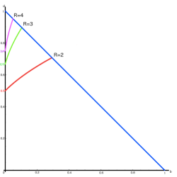
Figure 10: Parameter space of the phenotypic model. The blue line is boundary $b+d=1$. The red, green and magenta curves are the critical curves $\mu(b,d,R)=1$ for $R=2,3,4$, respectively.

In this parameter space one can consider the critical curves $\mu(b,d,R)=1$, where $\mu(b,d,R)$ is the malthusian parameter as a function of the parameters of the phenotypic model. For each fixed $R$, the corresponding critical curve is independent of the fitness distributions and represents the parameter values $(b,d)$ such that the branching process is critical. Moreover, each curve splits the simplex into two regions representing the parameter values where the branching process is super-critical (above the curve) and sub-critical (below the curve).

One of the main results of ABCJ13a is a proof of the lethal mutagenesis criterion BSW07 for the phenotypic model, provided one assumes that all fitness effects are of a purely mutational nature. Recall that BSW07 assumes that all mutations are either neutral or deleterious and consider the mutation rate $U=U_{d}+U_{c}$, where the component $U_{c}$ comprises the purely neutral mutations and the component $U_{d}$ comprises the mutations with a deleterious fitness effect. Furthermore, $R_{\mathrm{max}}$ denotes the maximum replicative capability among all particles in the viral population. The lethal mutagenesis criterion proposed by BSW07 states that a sufficient condition for extinction is

$$R_{\mathrm{max}}\,\mathrm{e}^{-U_{d}}<1\,.$$ (23)

According to BSW07 ; BSW08 , $\mathrm{e}^{-U_{d}}$ is both the mean fitness level and also the fraction of offspring with no non-neutral mutations. Moreover, in the absence of beneficial mutations and epistasis KM66 the only type of non-neutral mutations are the deleterious mutations. Therefore, in terms of fitness effects, the probability $\mathrm{e}^{-U_{d}}$ corresponds to $1-d=c$. Since the evolution of the mean matrix depends only on the expected values of the fitness distribution $t_{r}$, it follows that $R_{\mathrm{max}}$ corresponds to $R$. That is, the lethal mutagenesis criterion of (23) is formally equivalent to extinction criterion

$$R(1-d)<1$$ (24)

which is exactly the condition for the phenotypic model to become sub-critical. Formula (20) for the malthusian parameter provides a generalization of the extinction criterion (24) without the assumption that that all effects are either neutral or deleterious. If $b>0$ is sufficiently small (up to order $\bm{O}(b^{2})$) and

$$R\left((1-d)+(R-1)\dfrac{bd}{1-d}\right)<1$$ (25)

then, with probability one, the population becomes extinct in finite time.

On the other hand, a deeper exploration of the implications of non-zero beneficial effects allowed for the discovery of a non-extinction criterion. If $b>0$ is sufficiently small (up to order $\bm{O}(b^{2})$), $R$ is sufficiently large ($R\geqslant 10$ is enough) and

$$R^{3}\,b>1$$ (26)

then, asymptotically almost surely, the population can not become extinct by increasing the deleterious probability $d$ towards its maximum value $1-b$ (see ABCJ13a for details). In other words, a small increase of the beneficial probability may have a drastic effect on the extinction probabilities, possibly rendering the population impervious to become extinct by lethal mutagenesis (i.e., by increase of deleterious effects).

In the theory of multitype branching processes there several variations as follows: continuous time, age dependent, self-regulated, etc, (see AN72 ; H63 ; K02 ). The implementation of a variation of the theory of multitype branching process accounting for the notions of evolutionary entropy and directionality theory (see D05 ; D2013 ) could be useful for studies on viral evoltution. In this case, the malthusian parameter $\mu$, which is the dominant eigenvalue of the mean matrix, could be expressed as the sum of two terms

$$\mu=H+\Phi\,.$$

The quantity $H$ is called evolutionary entropy and $\Phi$ is called the reproductive potential D2013 . An interesting direction to follow would be to develop an extinction criterion based on evolutionary entropy instead of the malthusian parameter.

Appendix C The Deterministic Selection Equation

According to DSS85 ; D1985 ; D1987 , one may associate to a multitype branching process a system of difference (or ordinary differential) equations, called selection equations, on the space of discrete probability distributions $\triangle^{R+1}=\{\bm{p}\in\mathbb{R}^{R+1}:p_{j}\geqslant 0;\sum_{j}p_{j}=1\}$ over the finite state set $\{0,\ldots,R\}$. Given a discrete multitype branching process $\bm{Z}_{n}$, then the expectation values $\langle\bm{Z}_{n}\rangle$ satisfy $\langle\bm{Z}_{n}\rangle=\bm{M}^{n}\bm{Z}_{0}$, with $\bm{M}$ being the mean matrix of $\bm{Z}_{n}$. Hence $\bm{Z}_{n}$ is given by iteration of the difference equation $\bm{z}_{n}=\bm{M}\bm{z}_{n-1}$. This yields a discrete-time selection equation by normalizing the difference equation, thereby obtaining

$$\bm{x}_{n}=\dfrac{1}{\bm{1}^{\mathrm{t}}\bm{M}\bm{x}_{n-1}}\bm{M}\bm{x}_{n-1}$$ (27)

where $\bm{1}=(1,\ldots,1)$. Then, passing (27) to continuous time one obtains a continuous-time selection equation

$$\dot{\bm{x}}=[\bm{M}\bm{x}-\bm{x}(\bm{1}^{\mathrm{t}}\bm{M}\bm{x})]\dfrac{1}{\bm{1}^{\mathrm{t}}\bm{M}\bm{x}}\,.$$ (28)

Multiplying the right hand side of equation (28) with the factor $\bm{1}^{\mathrm{t}}\bm{M}\bm{x}$, which is always strictly positive on $\triangle^{R+1}$, corresponds to a change in velocity (re-scaling time) and so, the solutions of (28) are the same as the solutions of

$$\dot{\bm{x}}=\bm{M}\bm{x}-\bm{x}(\bm{1}^{\mathrm{t}}\bm{M}\bm{x})$$ (29)

It follows from general considereations (see DSS85 ; D1985 ; D1987 ) that equation (29) has a unique global stable equilibrium on $\triangle^{R+1}$ given by the normalized right eigenvector $\bm{u}$ of $\bm{M}$ corresponding to its largest eigenvalue $\mu$. In this sense, the deterministic selection equation yields a description of the evolution of the normalized mean values of the corresponding stochastic model, thus definig a mean field (macroscopis) dynamics representing the infinite population limit of the branching process.

Appendix D The Power Law Distribution Family

It is typical to parameterize power law distributions by the exponent $s$, which measures the “weight of the tail” of the distribution. However, we need to have a location-scale parameterized family in order to impose the same normalization as we have done for the other types of distributions. Therefore, we define the power law distribution with mean value $r$ by

$$\mathfrak{z}_{r}(k)=\frac{(k-1)^{s(r)}}{\zeta(s(r))}$$

for $k=0,1,\ldots,\infty$ and $r\geqslant 1$, where $\zeta(s)$ is the Riemann zeta function, defined for $s>1$, by

$$\zeta(s)=\sum_{n=1}^{\infty}\frac{1}{n^{s}}$$

and the function $s(r)$ is given by the inverse function of

$$r=\varphi(s)=\frac{\zeta(s-1)}{\zeta(s)}-1\,.$$

Namely, $s=\varphi^{-1}(r)$ for $r\geqslant 1$ and hence when $1\leqslant r<\infty$ the exponent $s$ satisfies $3<s<2$. Moreover, the Laurent series expansion for $r\to\infty$ ($s\to 2$) is given by:

$$s(r)\approx 2+\frac{6}{\pi^{2}(1+r-C)}\,.$$ (30)

The constant $C$ in the previous formula is given by $C=[6\gamma\pi^{2}-36\,\zeta^{\prime}(2)]/\pi^{4}\approx 0.6974$, where $\gamma$ is Euler’s constant and $\zeta^{\prime}(2)$ is the derivative of $\zeta(s)$ evaluated at $2$. Observe that when the mean value $r\geqslant 1$, the exponent $s<3$, and so the variance of $\mathfrak{z}_{r}(k)$ is infinite.

The implementation of the pseudo-random generation of samples from the distribution $\mathfrak{z}_{r}(k)$ in the ENVELOPE program is based on the algorithm of D1986 for the Zipf distribution on the positive integers, using formula 30 for the computation of the exponent $s$ given the mean value $r$. Pseudo-random generation for the remaining fitness distributions were implemented using the standard library of C++ programing language (this library requires C++ (2011) or superior).

Appendix E Main Routines of the ENVELOPE Program

1:$\triangleright$ Variables Defined by the User

2:Real $b,d$; $\triangleright$ Beneficial and Deleterious Probabilities

3:Integer $R$; $\triangleright$ Maximum Replicative Cabability

4:Integer $N$; $\triangleright$ Maximum Generation Time

5:Integer $K$; $\triangleright$ Maximum Numer of Particles

6:Intehre $type$; $\triangleright$ Type of Fitness Distribution

7:Integer Vector $initial\_population[0,\ldots,R]$; $\triangleright$ Initial Particle Distribution

1:$\triangleright$ Global Variables

2:Integer Vector $malthusian[0,\ldots,N]$; $\triangleright$ Malthusian Parameter per Generation

3:Real Matrix $class\_distribution[0,\ldots,R][0,\ldots,N]$; $\triangleright$ Class Distribution per Generation

4:Real Vector $mean\_rho[0,\ldots,N]$; $\triangleright$ Average Reproduction Rate per Generation

5:Real Vector $diversity[0,\ldots,N]$; $\triangleright$ Phenotypic Diversity per Generation

6:Real Vector $entropy[0,\ldots,N]$; $\triangleright$ Phenotypic Entropy per Generation

1:$\triangleright$ Internal Variables

2:Integer $n$; $\triangleright$ Current Generation Time

3:Integer $T$; $\triangleright$ Current Total Progeney

4:Integer $progeny$; $\triangleright$ Progeney of a Replicative Class

5:Integer $sampled$; $\triangleright$ Random Particle Sampled

6:Integer Vector $particles[0,\ldots,R]$; $\triangleright$ Current Particle Distribution

7:Integer Vector $parents[0,\ldots,R]$; $\triangleright$ Current Parental Distribution

8:Integer Vector $next[0,\ldots,R]$; $\triangleright$ Next Generation Particle Distribution

9:Real effect; $\triangleright$ Random Number Between $0$ and $1$

1:$\triangleright$ Sample from a Fitness Distribution of type $t$ with mean value $m$

2:function FitnessDistribution(Real $m$, Integer $t$)

3:     Integer $value$;

4:     case $t$ do

5:     $t=0$: $value\leftarrow(\textrm{Integer})\,m$;

6:     $t=1$: $value\leftarrow\textsc{Poisson}(m)$;

7:     $t=2$: $value\leftarrow\textsc{Geometric}(1/(1+m))$;

8:     $t=3$: $value\leftarrow\textsc{Binomial}(2*m,1/2)$;

9:     $t=4$: $value\leftarrow\textsc{PowerLaw}(m)$;

10:     end case

11:     return $value$;

12:end function

1:$\triangleright$ Compute the Statistics for the Next Generation

2:procedure Statistics(Integer Vector $u$, Integer Vector $v$, Integer $n$)

3:     $malthusian[n]\leftarrow\textsc{Sum}(u)/\textsc{Sum}(v)$;

4:     for $i$ from $0$ to $R$ do

5:         $class\_distribution[i][n]\leftarrow v[i]/\textsc{Sum}(v)$;

6:     end for

7:     $mean\_rho[n]\leftarrow\textsc{Average}(class\_distribution[n])$;

8:     $diversity[n]\leftarrow\textsc{Diversity}(class\_distribution[n])$;

9:     $entropy[n]\leftarrow\textsc{Entropy}(class\_distribution[n])$;

10:end procedure

1:$\triangleright$ Average of Class Distribution

2:function Average(Real Vector $prob$)

3:     Real $x=0.0$;

4:     for $i$ from $1$ to $R$ do

5:         $x\leftarrow x+i*prob[i]$;

6:     end for

7:     return $x$;

8:end function

1:$\triangleright$ Diversity of Class Distribution

2:function Diversity(Real Vector $prob$)

3:     Real $x=0.0$, $y=0.0$;

4:     for $i$ from $1$ to $R$ do

5:         $x\leftarrow x+i*i*prob[i]$;

6:     end for

7:     $y\leftarrow\textsc{Average}(prob)$;

8:     $x\leftarrow x-y*y$;

9:     return $x$;

10:end function

1:$\triangleright$ Entropy of Class Distribution

2:function Entropy(Real Vector $prob$)

3:     Real $x=0.0$;

4:     for $i$ from $1$ to $R$ do

5:         $x\leftarrow x+prob[i]*\textsc{Log}(prob[i])$;

6:     end for

7:     return $x$;

8:end function

1:$\triangleright$ Initialization

2:$particles\leftarrow initial\_population$;

3:$n\leftarrow 0$;

4:$\triangleright$ Main loop

5:repeat

6:     $T\leftarrow\textsc{Sum}(particles)$;

7:     $parents\leftarrow particles$;

8:     $next\leftarrow[0,\ldots,0]$;

9:     for $i$ from $0$ to $R$ do $\triangleright$ Generate Progeny

10:         $progeny\leftarrow 0$;

11:         for $j$ from $1$ to $parents[i]$ do

12:              $progeny\leftarrow progeny+\textsc{FitnessDistribution}((\textrm{Real})\,i,type)$;

13:         end for

14:         $particles[i]\leftarrow progeny$;

15:     end for

16:     if $T<=K$ then $\triangleright$ Find Replicative Class of Progeny Without Cut Off

17:         for $i$ from $0$ to $R$ do

18:              for $j$ from $1$ to $particles[i]$ do

19:                  $\textit{effect}\leftarrow\textsc{RandomRealNumber}(0,1)$;

20:                  if $\textit{effect}<=d$ then $\triangleright$ Deleterious Effect

21:                       $next[i-1]\leftarrow next[i-1]+1$;

22:                  else if $\textit{effect}>d+b$ then $\triangleright$ Beneficial Effect

23:                       $next[i+1]\leftarrow next[i+1]+1$;

24:                  else$\triangleright$ Neutral Effect

25:                       $next[i]\leftarrow next[i]+1$;

26:                  end if

27:              end for

28:         end for

29:     else$\triangleright$ Find Replicative Class of Progeny With Cut Off

30:         for $j$ from $1$ to $K$ do

31:              $sampled\leftarrow\textsc{RandomIntegerNumber}(0,T)$;

32:              for $i$ from $0$ to $R$ do

33:                  if $sampled<particles[i]$ then

34:                       $T\leftarrow T-1$;

35:                       $particles[i]\leftarrow particles[i]-1$;

36:                       $\textit{effect}\leftarrow\textsc{RandomRealNumber}(0,1)$;

37:                       if $\textit{effect}<=d$ then $\triangleright$ Deleterious Effect

38:                           $next[i-1]\leftarrow next[i-1]+1$;

39:                       else if $\textit{effect}>d+b$ then $\triangleright$ Beneficial Effect

40:                           $next[i+1]\leftarrow next[i+1]+1$;

41:                       else$\triangleright$ Neutral Effect

42:                           $next[i]\leftarrow next[i]+1$;

43:                       end if

44:                       break;

45:                  else

46:                       $sampled\leftarrow sampled-particles[i]$;

47:                  end if

48:              end for

49:         end for

50:     end if

51:     $particles\leftarrow next$; $\triangleright$ Conclude and Sumarize

52:     $n\leftarrow n+1$;

53:     Statistics($parents$,$next$,$n$);

54:until $T=0$ or $n>N$ or UserStop;

References

- (1) Alberch, P.: From genes to phenotype: dynamical systems and evolvability. Genetica 84(1), 5–11 (1991)
- (2) Antoneli, F., Bosco, F.A.R., Castro, D., Janini, L.M.R.: Viral evolution and adaptation as a multivariate branching process. In: R.P. Mondaini (ed.) BIOMAT 2012 – Proceedings of the International Symposium on Mathematical and Computational Biology, vol. 13, pp. 217–243. World Scientific (2013). DOI 10.1142/9789814520829˙0013
- (3) Antoneli, F., Bosco, F.A.R., Castro, D., Janini, L.M.R.: Virus replication as a phenotypic version of polynucleotide evolution. Bulletin of Mathematical Biology 75(4), 602–628 (2013). DOI 10.1007/s11538-013-9822-9
- (4) Athreya, K.B., Ney, P.E.: Branching Processes. Springer-Verlag, Berlin (1972)
- (5) Bergstrom, C.T., McElhany, P., Real, L.A.: Transmission bottlenecks as determinants of virulence in rapidly evolving pathogens. Proceedings of the National Academy of Sciences 96(9), 5095–5100 (1999)
- (6) Bradwell, K., Combe, M., Domingo-Calap, P., Sanjuán, R.: Correlation between mutation rate and genome size in riboviruses: mutation rate of bacteriophage Q. Genetics 195(1), 243–251 (2013)
- (7) Bull, J.J., Sanjuán, R., Wilke, C.O.: Theory of lethal mutagenesis for viruses. J. Virology 18(6), 2930–2939 (2007). DOI 10.1128/JVI.01624-06
- (8) Bull, J.J., Sanjuán, R., Wilke, C.O.: Lethal mutagenesis. In: E. Domingo, C.R. Parrish, J.J. Holland (eds.) Origin and Evolution of Viruses, second edition edn., chap. 9, pp. 207–218. Academic Press, London (2008). DOI 10.1016/B978-0-12-374153-0.00009-6
- (9) Burch, C.L., Chao, L.: Epistasis and its relationship to canalization in the RNA virus 6. Genetics 167(2), 559–567 (2004)
- (10) Burch, C.L., Guyader, S., Samarov, D., Shen, H.: Experimental estimate of the abundance and effects of nearly neutral mutations in the RNA virus 6. Genetics 176(1), 467–476 (2007)
- (11) Campbell, R.B.: A logistic branching process for population genetics. Journal of Theoretical Biology 225(2), 195–203 (2003)
- (12) Carrasco, P., de la Iglesia, F., Elena, S.F.: Distribution of fitness and virulence effects caused by single-nucleotide substitutions in Tobacco Etch virus. J. Virology 18(23), 12,979–12,984 (2007)
- (13) Cerf, R.: Critical population and error threshold on the sharp peak landscape for a Moran model. Mem. Amer. Math. Soc. 233(1096), 1–87 (2015)
- (14) Cerf, R.: Critical population and error threshold on the sharp peak landscape for the Wright–Fisher model. The Annals of Applied Probability 25(4), 1936–1992 (2015)
- (15) Cerf, R., Dalmau, J.: The distribution of the quasispecies for a Moran model on the sharp peak landscape. Stochastic Processes and their Applications 126(6), 1681–1709 (2016)
- (16) Cuesta, J.A.: Huge progeny production during transient of a quasi-species model of viral infection, reproduction and mutation. Math. Comp. Model. 54, 1676–1681 (2011). DOI 10.1016/j.mcm.2010.11.055
- (17) Cuevas, J.M., Duffy, S., Sanjuán, R.: Point mutation rate of bacteriophage X174. Genetics 183, 747–749 (2009)
- (18) Dalmau, J.: The distribution of the quasispecies for the Wright–Fisher model on the sharp peak landscape. Stochastic Processes and their Applications 125(1), 272–293 (2015)
- (19) Dalmau, J.: Distribution of the quasispecies for a Galton–Watson process on the sharp peak landscape. Journal of Applied Probability 53(02), 606–613 (2016)
- (20) Demetrius, L.: The units of selection and measures of fitness. Proc. R. Soc. Lond. B 225(1239), 147–159 (1985)
- (21) Demetrius, L.: An extremal principle of macromolecular evolution. Physica Scripta 36(4), 693 (1987)
- (22) Demetrius, L.: Boltzmann, Darwin and directionality theory. Physics Reports 530(1), 1–85 (2013)
- (23) Demetrius, L., Schuster, P., Sigmund, K.: Polynucleotide evolution and branching processes. Bull. Math. Biol. 47(2), 239–262 (1985)
- (24) Devroye, L.: Non-uniform random variate generation. Springer-Verlag (1986)
- (25) Di Mascio, M., Markowitz, M., Louie, M., Hogan, C., Hurley, A., Chung, C., Ho, D.D., Perelson, A.S.: Viral blip dynamics during highly active antiretroviral therapy. Journal of Virology 77(22), 12,165–12,172 (2003)
- (26) Dietz, K.: Darwinian fitness, evolutionary entropy and directionality theory. BioEssays 27, 1097–1101 (2005)
- (27) Domingo, E., Holland, J.J.: RNA virus mutations and fitness for survival. Annual Reviews in Microbiology 51(1), 151–178 (1997)
- (28) Domingo, E., Martin, V., Perales, C., Grande-Perez, A., Garcia-Arriaza, J., Arias, A.: Viruses as quasispecies: biological implications. In: Quasispecies: Concept and Implications for Virology, pp. 51–82. Springer (2006)
- (29) Domingo, E., Martínez-Salas, E., Sobrino, F., de la Torre, J.C., Portela, A., Ortín, J., López-Galindez, C., Pérez-Breña, P., Villanueva, N., Nájera, R.: The quasispecies (extremely heterogeneous) nature of viral RNA genome populations: biological relevance – a review. Gene 40(1), 1–8 (1985)
- (30) Domingo, E., Sabo, D., Taniguchi, T., Weissmann, G.: Nucleotide sequence heterogeneity of an RNA phage population. Cell 13, 635–744 (1978)
- (31) Domingo-Calap, P., Cuevas, J.M., Sanjuán, R.: The fitness effects of random mutations in single-stranded DNA and RNA bacteriophages. PLoS Genetics 5(11), e1000,742 (2009)
- (32) Drake, J.W.: A test of Kimura’s mutation-rate conjecture. In: Radiobiology and Environmental Security, pp. 13–18. Springer (2012)
- (33) Eigen, M.: Selforganization of matter and the evolution of biological macromolecules. Naturwissenschaften 58, 465–523 (1971)
- (34) Eigen, M.: Viral quasispecies. Sci. Am. 269, 42–49 (1993)
- (35) Eigen, M., Schuster, P.: The Hypercycle. A principle of natural self-organization. Springer-Verlag, Berlin (1979)
- (36) Feller, W.: An Introduction to Probability Theory and Its Applications, vol. 1, third edn. Wiley, New York (1968)
- (37) Fiebig, E.W., Wright, D.J., Rawal, B.D., Garrett, P.E., Schumacher, R.T., Peddada, L., Heldebrant, C., Smith, R., Conrad, A., Kleinman, S.H., Busch, M.P.: Dynamics of HIV viremia and antibody seroconversion in plasma donors: implications for diagnosis and staging of primary HIV infection. Aids 17(13), 1871–1879 (2003)
- (38) Fortuna, M.A., Zaman, L., Ofria, C., Wagner, A.: The genotype-phenotype map of an evolving digital organism. PLoS computational biology 13(2), e1005,414 (2017)
- (39) Furió, V., Moya, A., Sanjuán, R.: The cost of replication fidelity in an RNA virus. Proceedings of the National Academy of Sciences of the United States of America 102(29), 10,233–10,237 (2005)
- (40) Gallant, J.E.: Making sense of blips. Journal of Infectious Diseases 196(12), 1729–1731 (2007)
- (41) Gupta, V., Dixit, N.M.: Scaling law characterizing the dynamics of the transition of HIV-1 to error catastrophe. Physical biology 12(5), 054,001 (2015)
- (42) Harris, T.E.: The Theory of Branching Processes. Springer-Verlag, Berlin (1963)
- (43) Jagers, P., Klebaner, F.C., Sagitov, S.: On the path to extinction. Proc. Natl. Acad. Sci. U. S. A. 104(15), 6107–6111 (2007)
- (44) Kesten, H., Stigum, B.P.: Additional limit theorems for indecomposable multidimensional Galton-Watson processes. Ann. Math. Stat. 37(6), 1463–1481 (1966)
- (45) Kesten, H., Stigum, B.P.: A limit theorem for multidimensional Galton-Watson processes. Ann. Math. Stat. 37(5), 1211–1223 (1966)
- (46) Kesten, H., Stigum, B.P.: Limit theorems for decomposable multi-dimensional Galton-Watson processes. J. Math. Anal. Appl. 17, 309–338 (1967)
- (47) Kimmel, M., Axelrod, D.E.: Branching Processes in Biology. Springer-Verlag, New York (2002)
- (48) Kimura, M., Maruyama, T.: The mutational load with epistatic gene interactions in fitness. Genetics 54(6), 1337 (1966)
- (49) Kurtz, T.G., Lyons, R., Pemantle, R., Peres, Y.: A conceptual proof of the Kesten-Stigum theorem for multi-type branching processes. In: K. Athreya, P. Jagers (eds.) Classical and Modern Branching Processes, IMA Vol. Math. Appl., vol. 84, pp. 181–185. Springer-Verlag, New York (1994)
- (50) Lambert, A.: The branching process with logistic growth. The Annals of Applied Probability 15(2), 1506–1535 (2005)
- (51) Lee, P.K., Kieffer, T.L., Siliciano, R.F., Nettles, R.E.: HIV-1 viral load blips are of limited clinical significance. Journal of Antimicrobial Chemotherapy 57(5), 803–805 (2006)
- (52) Loeb, L.A., Essigmann, J.M., Kazazi, F., Zhang, J., Rose, K.D., Mullins, J.I.: Lethal mutagenesis of HIV with mutagenic nucleoside analogs. Proc. Natl. Acad. Sci. U. S. A. 96, 1492–1497 (1999)
- (53) Lotka, A.J.: Théorie analytique des associations biologiques. Part II. analyse démographique avec application particuliere al’espece humaine. Actualités Scientifiques et Industrielles 780, 123—136 (1939)
- (54) Lynch, M., Bürger, R., Butcher, D., Gabriel, W.: The mutational meltdown in asexual populations. Journal of Heredity 84(5), 339–344 (1993)
- (55) Lynch, M., Gabriel, W.: Mutation load and the survival of small populations. Evolution pp. 1725–1737 (1990)
- (56) Manrubia, S.C., Lázaro, E., Pérez-Mercader, J., Escarmís, C., Domingo, E.: Fitness distributions in exponentially growing asexual populations. Phys. Rev. Lett. 90(18), 188,102 (2003)
- (57) Matuszewski, S., Ormond, L., Bank, C., Jensen, J.D.: Two sides of the same coin: A population genetics perspective on lethal mutagenesis and mutational meltdown. Virus Evolution 3(1) (2017)
- (58) McMichael, A.J., Borrow, P., Tomaras, G.D., Goonetilleke, N., Haynes, B.F.: The immune response during acute HIV-1 infection: clues for vaccine development. Nature Reviews Immunology 10(1), 11–23 (2010)
- (59) Mode, C.J., Sleeman, C.K.: Stochastic processes in genetics and evolution: computer experiments in the quantification of mutation and selection. World Scientific (2012)
- (60) Mode, C.J., Sleeman, C.K., Raj, T.: On the inclusion of self regulating branching processes in the working paradigm of evolutionary and population genetics. Frontiers in Genetics 4 (2013)
- (61) Nagaev, A.V.: On estimating the expected number of direct descendants of a particle in a branching process. Theory of Probability & Its Applications 12(2), 314–320 (1967)
- (62) Nettles, R.E., Kieffer, T.L.: Update on HIV-1 viral load blips. Current Opinion in HIV and AIDS 1(2), 157–161 (2006)
- (63) Nettles, R.E., Kieffer, T.L., Kwon, P., Monie, D., Han, Y., Parsons, T., Cofrancesco, J., Gallant, J.E., Quinn, T.C., Jackson, B.: Intermittent HIV-1 viremia (blips) and drug resistance in patients receiving HAART. Jama 293(7), 817–829 (2005)
- (64) Peris, J.B., Davis, P., Cuevas, J.M., Nebot, M.R., Sanjuán, R.: Distribution of fitness effects caused by single-nucleotide substitutions in bacteriophage F1. Genetics 185(2), 603–609 (2010)
- (65) Rong, L., Perelson, A.S.: Asymmetric division of activated latently infected cells may explain the decay kinetics of the HIV-1 latent reservoir and intermittent viral blips. Mathematical Biosciences 217(1), 77–87 (2009)
- (66) Rong, L., Perelson, A.S.: Modeling HIV persistence, the latent reservoir, and viral blips. Journal of Theoretical Biology 260(2), 308–331 (2009)
- (67) Sanjuán, R., Moya, A., Elena, S.F.: The distribution of fitness effects caused by single-nucleotide substitutions in an RNA virus. Proc. Natl. Acad. Sci. U. S. A. 101, 8396–8401 (2004)
- (68) Schuster, P., Swetina, J.: Stationary mutant distributions and evolutionary optimization. Bulletin of mathematical biology 50(6), 635–660 (1988)
- (69) Servedio, M.R., Brandvain, Y., Dhole, S., Fitzpatrick, C.L., Goldberg, E.E., Stern, C.A., Cleve, J.V., Yeh, D.J.: Not just a theory – the utility of mathematical models in evolutionary biology. PLoS Biology 12(12), e1002,017 (2014). DOI 10.1371/journal.pbio.1002017
- (70) Swetina, J., Schuster, P.: Self-replication with errors: a model for polynucleotide replication. Biophysical Chemistry 16(4), 329–345 (1982). DOI 10.1016/0301-4622(82)87037-3
- (71) Takeuchi, N., Hogeweg, P.: Error-threshold exists in fitness landscapes with lethal mutants. BMC Evolutionary Biology 7(1), 15 (2007)
- (72) Tromas, N., Elena, S.F.: The rate and spectrum of spontaneous mutations in a plant RNA virus. Genetics 185(3), 983–989 (2010)
- (73) Watson, H.W., Galton, F.: On the probability of the extinction of families. J. Anthropol. Inst. Great Britain and Ireland 4, 138–144 (1874)
- (74) Wilke, C.O.: Quasispecies theory in the context of population genetics. BMC Evolutionary Biology 5(1), 44 (2005)
- (75) Zhu, Y., Yongky, A., Yin, J.: Growth of an RNA virus in single cells reveals a broad fitness distribution. Virology 385(1), 39–46 (2009). DOI 10.1016/j.virol.2008.10.031