Stochastic Gradient MCMC Methods for Hidden Markov Models

Abstract

Stochastic gradient MCMC (SG-MCMC) algorithms have proven useful in scaling Bayesian inference to large datasets under an assumption of i.i.d data. We instead develop an SG-MCMC algorithm to learn the parameters of hidden Markov models (HMMs) for time-dependent data. There are two challenges to applying SG-MCMC in this setting: The latent discrete states, and needing to break dependencies when considering minibatches. We consider a marginal likelihood representation of the HMM and propose an algorithm that harnesses the inherent memory decay of the process. We demonstrate the effectiveness of our algorithm on synthetic experiments and an ion channel recording data, with runtimes significantly outperforming batch MCMC.

1 Introduction

Stochastic gradient based algorithms have proven crucial in numerous areas for scaling inference algorithms to large datasets. The key idea is to employ noisy estimates of the gradient based on minibatches of data, avoiding a costly gradient computation using the full dataset (Robbins & Monro, 1951). Assuming the data are i.i.d. and the minibatches are properly scaled, the stochastic gradient is an unbiased estimate of the true gradient. In the context of Bayesian inference, such approaches have proven useful in scaling variational inference (Hoffman et al., 2013; Bryant & Sudderth, 2012; Broderick et al., 2013; Foti et al., 2014) and Markov chain Monte Carlo (MCMC) (Welling & Teh, 2011; Patterson & Teh, 2013; Chen et al., 2014; Ding et al., 2014; Shang et al., 2015). For the latter, a primary focus has been on the influence of the stochastic gradient noise on the MCMC iterates; in contrast to many optimization-based procedures, it is non-trivial to show that the underlying (stochastic) dynamics maintain the correct stationary distribution in the presence of such noise. Significant headway has been made in developing such correct SG-MCMC procedures. These algorithms have shown great practical benefits and have gained significant traction.

A separate challenge, however, is the important and often overlooked question of whether such stochastic gradient techniques can be applied to massive amounts of sequential or otherwise non-i.i.d. data. In such cases, crucial dependencies must be broken to form the necessary minibatches. This question received some attention in the stochastic variational inference (SVI) algorithm of Foti et al. (2014) for hidden Markov models (HMMs). In this work, we also focus in on HMMs as a simple example of a sequential data model, but turn our attention to SG-MCMC algorithms.

There are many existing algorithms for inferring the model parameters of an HMM including Monte Carlo methods (Scott, 2002), expectation-maximization (EM) (Bishop, 2006), and variational algorithms (Beale, 2003). All of these ideas operate by iterating between a local update for the latent states, followed by a global update of the model parameters. The local update is usually performed using the forward-backward algorithm that allows computation of any marginal, or pair-wise marginal, in time linear in the length of the sequence.

In the variational context, recent work has focused on scaling these local-global inference schemes to settings with a large number of replicates of short sequences (Johnson & Willsky, 2014; Hughes et al., 2015). These methods utilize the fact that independent replicates of the observation sequence can be used to compute unbiased gradient estimates (Johnson & Willsky, 2014), and can be used to incrementally update sufficient statistics (Hughes et al., 2015). In contrast, the SVI-HMM algorithm of Foti et al. (2014) examines how to deal with extremely long observation sequences. The algorithm heuristically breaks the dependence between observations and performs local updates on short subsequences of observations using a limited forward-backward algorithm. These existing methods suffer from a number of drawbacks. The variational approaches must use an approximate posterior distribution for both the state- and model-parameters, which may not be representative of the true distributions. The methods are also limited to conjugate prior distributions over the parameters, which can severely limit the expressiveness of the model. Finally, all of the methods discussed thus far are susceptible to the widely known problem of underestimating posterior correlations biasing fully Bayesian analyses.

Unfortunately, attempting to naively use subchains as in Foti et al. (2014) within SG-MCMC approaches is fraught with difficulty: The local-global structure of SVI-HMM does not lend itself to deriving provably correct SG-MCMC algorithms, stemming from two main challenges.

The first challenge is that SG-MCMC methods sample continuous-valued parameter representations, whereas the HMM learning objective is typically specified in terms of the discrete-valued state sequence (local variables). To address this challenge, we consider an alternative approach to performing parameter inference for HMMs: We work directly with the marginal likelihood of the observation. We form stochastic gradients by only evaluating terms of the full gradient that depend on a small subsequence.

The second challenge is handling the temporal dependencies, specifically: i) each subsequence-specific term in the stochastic gradient still requires a forward-backward pass on the rest of the sequence, and ii) proximal subsequences are mutually correlated. We address both of these issues by capitalizing on the well-known memory decay of the Markovian structure underlying the data generating process. Specifically, we approximate the full forward-backward passes with message passing only on short buffers around the considered subsequences of observations. We further restrict subsequences to be sufficiently far from one another to ensure that computations with them are uncorrelated. We provide a theoretically justified approach to estimating this buffer length and between-subsequence gap, allowing us to prove the validity of the resulting SG-MCMC algorithm. In particular, the same theoretical guarantees are provided as in the i.i.d. setting.

Buffering to perform limited message passing in HMMs was also applied in SVI-HMM Foti et al. (2014); however, the buffering there was part of a latent state update. In particular, SVI-HMM iterates between buffered message passing for local updates and stochastic gradients for global updates. We, in contrast, consider stochastic gradients of a marginal likelihood representation and utilize buffering directly within this stochastic gradient calculation.

We evaluate the efficacy of our buffered SG-MCMC method for HMMs on two synthetic examples with very different dynamics. We compare against an unbuffered SG-MCMC approach as well as against treating the data as i.i.d. Finally, we show the computational gains of our SG-MCMC algorithm over batch MCMC by segmenting an ion channel dataset where a 1,000X speedup was observed. Collectively, our contributions make a sizable step towards general purpose SG-MCMC algorithms for sequential data.

2 Background

2.1 Hidden Markov Models

Hidden Markov models (HMMs) are a class of discrete-time doubly stochastic processes consisting of a i) latent discrete-valued state sequence $x_{t}\in\{1,\ldots,K\}$ generated by a Markov chain and (ii) corresponding observations $y_{t}$ generated from distributions determined by the latent states $x_{t}$. Specifically, the joint distribution of $\mathbf{y}=(y_{1},\cdots,y_{T})$ and $\mathbf{x}=(x_{0},\cdots,x_{T})$, factorizes as

$$p(\mathbf{x},\mathbf{y})=\pi_{0}(x_{0})\prod_{t=1}^{T}p(x_{t}|x_{t-1},A)\cdot p(y_{t}|x_{t},\phi),$$ (1)

where $A$ is the Markov transition matrix such that $A_{i,j}=\Pr(x_{t}=i|x_{t-1}=j)$, $\{\phi_{k}\}^{K}_{k=1}$ are the emission parameters, and $\pi_{0}=p(x_{0})$ is the initial state distribution. We denote the parameters of interest as $\theta=\{A,\phi\}$ and do not focus on performing inference on $\pi_{0}$.

Traditionally, EM, variational inference, or MCMC are used to perform inference over $\theta$ (Scott, 2002; Beale, 2003). These algorithms rely on the well-known forward-backward algorithm to compute the marginal, $p(x_{t}|y_{1:T})$, and pairwise-marginal, $p(x_{t},x_{t+1}|y_{1:T})$, distributions. The algorithm works by recursively computing a sequence of forward messages $\alpha_{t}(x_{t})=p(x_{t}|y_{1:t})$ and backwards messages $\beta_{t}(x_{t})=p(y_{t+1:T}|x_{t})$ which can then be used to compute the necessary marginals (Beale, 2003). These marginals are then used to update or sample from the distribution of the model parameters.

These past algorithms have found widespread use in statistics and machine learning. However, as discussed in Sec. 1, an alternative formulation of the HMM can provide greater utility in developing an SG-MCMC approach. Marginalizing over $\mathbf{x}$, we obtain the marginal likelihood:

$$p(\mathbf{y}|\theta)=\mathbf{1}^{\rm T}\ P(y_{T})A\cdots P(y_{1})A\ \mbox{\boldmath$\pi$}_{0},$$ (2)

where $P(y_{t})$ is a diagonal matrix with $P_{i,i}(y_{t})=p(y_{t}|x_{t}=i,\phi_{i})$; $\mathbf{1}^{\rm T}$ is a row vector of $K$ ones; and $(\mbox{\boldmath$\pi$}_{0})_{i}=\pi_{0}(x_{0}=i)$. The resulting posterior distribution of $\theta$ given $\mathbf{y}=y_{1:T}$ is then:

$$p(\theta|\mathbf{y}) \propto\mathbf{1}^{\rm T}\ P(y_{T})A\cdots P(y_{1})A\ \mbox{\boldmath$\pi$}_{0}\cdot p(\theta).$$ (3)

Working with the marginal likelihood and posterior alleviates the need to compute the marginals and pairwise marginals of $x_{t}$. As such, only the forward pass of the forward-backward algorithm is performed. Indeed, performing the matrix multiplications in Eq. (2) from right to left corresponds to computing the normalizing constants of the forward messages. Performing the matrix multiplies from left to right corresponds to unnormalized messages in belief propagation, (cf. Fox, 2009). Perhaps most importantly for the development of our SG-MCMC algorithm, the marginal likelihood does not involve alternately updating the local state variables, $x_{t}$, and the global model parameters $\theta$. Instead, we need only explore a continuous space which will allow us to leverage gradient information to develop a computationally and statistically efficient algorithm. The major impediment to directly using Eq. (2) for SG-MCMC is that it is unclear how to form a stochastic gradient based on a subsequence to avoid the computational burden of gradient computations in large $T$ settings.

2.2 Stochastic Gradient MCMC for i.i.d. Data

One approach for devising MCMC algorithms is to utilize continuous dynamics to explore a potential function $U(\theta)\propto-\ln\pi(\theta)$ for target distribution $\pi(\theta)$; for Bayesian inference, we take $U(\theta)\propto-\ln p(\theta|\mathbf{y})$, i.e., the negative log posterior. Then, samples of a continuous valued parameter, $\theta\in\mathbb{R}^{d}$, can be drawn as (Ma et al., 2015, 2016)

$$\theta^{(t+1)}\leftarrow \theta^{(t)}-\epsilon_{t}\left[\big{(}{\mathbf{D}}(\theta^{(t)})+{\mathbf{Q}}(\theta^{(t)})\big{)}\nabla{U}(\theta^{(t)})+\Gamma(\theta^{(t)})\right]$$

$$+\mathcal{N}(0,\epsilon_{t}(2\mathbf{D}(\theta^{(t)}))),$$ (4)

where $\Gamma_{i}(\theta)=\sum_{j=1}^{d}\dfrac{\partial}{\partial\theta_{j}}(\mathbf{D}_{i,j}(\theta)+\mathbf{Q}_{i,j}(\theta))$, ${\mathbf{D}}(\theta^{(t)})$ is a positive-definite matrix and ${\mathbf{Q}}(\theta^{(t)})$ a skew-symmetric matrix. Ma et al. (2015) proved that in the limit $\epsilon_{t}\rightarrow 0$ with ergodicity, the iterates $\theta^{(t)}$ will be drawn from $p(\theta|\mathbf{y})$.

For i.i.d. data, ${U}(\theta)=-\sum_{{s}\in{\mathcal{S}}}\ln p({y_{s}}|\theta)-\log p(\theta)$. For independently sampled data subsets, $\widetilde{\mathcal{S}}\subset\mathcal{S}$, a noisy unbiased estimate of the potential function is given by:

$$\widetilde{U}(\theta)=-\dfrac{|\mathcal{S}|}{|\widetilde{\mathcal{S}}|}\sum_{s\in\widetilde{\mathcal{S}}}\log p({y_{s}}|\theta)-\log p(\theta);\quad\widetilde{\mathcal{S}}\subset\mathcal{S}.$$ (5)

As such, a gradient computed based on $\widetilde{U}(\theta)$—called a stochastic gradient—is a noisy, but unbiased estimator of the full-data gradient. The key question is whether the noise injected by the stochastic gradient adversely affects the stationary distribution of the modified dynamics (using $\nabla\widetilde{U}(\theta)$ in place of $\nabla U(\theta)$). One way to analyze the impact of the stochastic gradient is to make use of the central limit theorem and assume

$$\nabla\widetilde{U}(\theta)=\nabla U(\theta)+\mathcal{N}(0,\mathbf{V}(\theta)).$$ (6)

Simply using $\nabla\widetilde{U}(\theta)$ in place of $\nabla U(\theta)$ in Eq. (4) results in an additional noise term $({\mathbf{D}}(\theta)+{\mathbf{Q}}(\theta)\big{)}\ \mathcal{N}(0,\mathbf{V}(\theta))^{T}$. Assuming we have an estimate $\widehat{\mathbf{B}}$ of the variance of this additional noise satisfying $2\mathbf{D}(\theta)-\epsilon\widehat{\mathbf{B}}\succeq 0$ (i.e., positive semidefinite), then we can attempt to account for the stochastic gradient noise by simulating

$$\theta^{(t+1)}\leftarrow \theta^{(t)}-\epsilon_{t}\left[\big{(}{\mathbf{D}}(\theta^{(t)})+{\mathbf{Q}}(\theta^{(t)})\big{)}\nabla\widetilde{U}(\theta^{(t)})+\Gamma(\theta^{(t)})\right]$$

$$+\mathcal{N}(0,\epsilon_{t}(2\mathbf{D}(\theta^{(t)})-\epsilon_{t}\widehat{\mathbf{B}}^{(t)})).$$ (7)

This is the SG-MCMC algorithm for i.i.d. data proposed by Ma et al. (2015, 2016). See Alg. 2.

For this SG-MCMC, there are sources of error introduced via (i) discretizing the continuous stochastic dynamics and (ii) estimation of the stochastic gradient noise covariance. Although the algorithm is provably correct as $\epsilon_{t}\rightarrow 0$, in practice one uses a small, finite stepsize for greater efficiency. In such cases, bias is introduced. This bias-variance tradeoff was recently studied in (Vollmer et al., 2016). Higher order numerical schemes (Chen et al., 2015; Leimkuhler & Shang, 2016) and a moving window estimation of $\widehat{B}$ can further reduce this bias (Shang et al., 2015).

Algorithm 1 SG-MCMC

  initialize $\theta_{0}$

  for $t=0,1,2\cdots,N_{iter}$ do

     for $i=1\cdots n$ do

         $\Gamma_{i}(\theta)=\sum_{j}\dfrac{\partial}{\partial\theta_{j}}\left({\mathbf{D}}_{ij}(\theta)+{\mathbf{Q}}_{ij}(\theta)\right)$

     end for

     sample $\eta^{(t)}\sim\mathcal{N}(0,2\epsilon_{t}\mathbf{D}(\theta^{(t)})-\epsilon_{t}^{2}\widehat{\mathbf{B}}^{(t)})$

      $\begin{array}[]{cl}\theta^{(t+1)}\leftarrow&\theta^{(t)}+\eta^{(t)}\\ &-\epsilon_{t}\left[\big{(}{\mathbf{D}}(\theta^{(t)})+{\mathbf{Q}}(\theta^{(t)})\big{)}\nabla\widetilde{U}(\theta^{(t)})+\Gamma(\theta^{(t)})\right]\end{array}$

  end for

3 Stochastic Gradient MCMC for HMMs

In order to apply SG-MCMC methods to HMMs we must be able to efficiently estimate the gradient of the potential, $U(\theta)\propto-\ln p(\theta|\mathbf{y})$. The approach we take consists of three steps (see Fig. 1). First, we marginalize out the discrete state sequence and use the marginal likelihood of the data. Next, we derive an expression for the gradient of the marginal likelihood that factorizes over disjoint subsequences. Finally, we compute an unbiased noisy estimate of the gradient by randomly sampling subsequences and show that using this estimate results in an SG-MCMC algorithm that admits the desired stationary distribution under the same conditions as in the i.i.d. case (see Sec. 2.2).

One could have imagined an alternative approach—as in SVI-HMM—of first sampling subsequences; we could then compute an approximation of the marginal likelihood on this subsequence and treat its gradient as our stochastic gradient. However, without the marginal likelihood information in the first place, it is not obvious how subsequences correlate with each other and consequently how to control the error resulting from subsampling.

3.1 Gradient of Marginal Likelihood Representation

Recall that the posterior under an HMM is given by Eq. (3) and that the potential function $U(\theta)\propto-\ln p(\theta|\mathbf{y})$. As will prove useful in our SG-MCMC algorithm, we rewrite the posterior in terms of a subsequence $\mathbf{y}_{\tau,L}=(y_{\tau-L},\ldots,y_{\tau},\ldots,y_{\tau+L})$ with half-width $L$ centered at time $\tau\in\{L+1,\ldots,T-L-1\}$. The overall subsequence length is $2L+1$. Defining

$$P(\mathbf{y}_{\tau,L})=P(y_{\tau+L})A\cdots P(y_{\tau-L})A,$$ (8)

we can rewrite Eq. (3) as

$$p(\theta|\mathbf{y}) \propto\mathbf{q}_{\tau+L+1}^{\rm T}P(\mathbf{y}_{\tau,L})\mbox{\boldmath$\pi$}_{\tau-L-1}\cdot p(\theta).$$ (9)

Here, $\mathbf{q}_{\tau+L+1,i}=p(\mathbf{y}_{\tau+L+1:T}|x_{\tau+L}=i)$ is the likelihood of the observations after $\mathbf{y}_{\tau,L}$ given the value of the latent state at $\tau$, and $\mbox{\boldmath$\pi$}_{\tau-L-1,i}=p(x_{\tau-L}=i|y_{1:\tau-L-1})$ is the predictive distribution of the latent state at $\tau$ given the observations before $\mathbf{y}_{\tau,L}$. Note, we do not actually need to instantiate the latent state variables $x_{\tau-L}$ and $x_{\tau+L+1}$ as $\mathbf{q}_{\tau+L+1}$ and $\mbox{\boldmath$\pi$}_{\tau-L-1}$ can be computed (in theory) via the forward-backward algorithm (Rabiner, 1989; Scott, 2002).

Let $\mathcal{S}=\{\mathbf{y}_{\tau,L}\}$ be a set of non-overlapping subsequences that cover $\mathbf{y}$. The gradient of Eq. (23) can be written as

$$\nabla U(\theta)_{i}=-\dfrac{\partial\ln p(\mathbf{y}|\theta)}{\partial\theta_{i}}-\dfrac{\partial\ln p(\theta)}{\partial\theta_{i}}$$ (10)

$$=-\sum_{\mathbf{y}_{\tau,L}\in\mathcal{S}}\dfrac{\mathbf{q}_{\tau+L+1}^{\rm T}\dfrac{\partial P(\mathbf{y}_{\tau,L})}{\partial\theta_{i}}\mbox{\boldmath$\pi$}_{\tau-L-1}}{\mathbf{q}_{\tau+L+1}^{\rm T}P(\mathbf{y}_{\tau,L})\mbox{\boldmath$\pi$}_{\tau-L-1}}-\dfrac{\partial\ln p(\theta)}{\partial\theta_{i}},$$

where the equality follows from the product rule (see the Supplement for complete derivation). Importantly, note that the gradient involves a sum over terms corresponding to all non-overlapping subsequences of length $2L+1$.

We could imagine using $\nabla U(\theta)$ from Eq. (A) in the update rule of Eq. (4) to generate sample values of $\theta$. However, Eq. (A) is extremely computationally intensive for two reasons. First, calculating $\mathbf{q}_{\tau+L+1}$ and $\mbox{\boldmath$\pi$}_{\tau-L-1}$ involves the whole sequence of length $T$. Second, one must compute $\mathbf{q}_{\tau+L+1}$, $P(\mathbf{y}_{\tau,L})$, and $\mbox{\boldmath$\pi$}_{\tau-L-1}$ for each $\mathbf{y}_{\tau,L}\in\mathcal{S}$ in the sum; this involves $T/L$ terms, thus requiring $O(T^{2})$ computation time to compute the gradient.

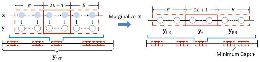
Figure 1: Diagram of subsequences, buffers, and subsequence sampling from full observation sequence. Left: The SVI method of Foti et al. (2014) approximates stochastic gradients using subchains of length $2L+1$ using the forward-backward algorithm performed on both the subchains and the associated buffer chains of length $B$. Right: Our propsoed SG-MCMC method uses a similar subsampling approach, however, i) the latent chain is never instantiated and ii) a minimum gap between consecutive subchains, $\mathbf{y}_{\tau,L}$, is used to ensure nearly uncorrelated subsequences. The thick black lines through the observables $\mathbf{y}$ represent all pairwise correlations between observations due to marginalization of $\mathbf{x}$. Correlation decays with distance enabling the segmentation of the of the chain into subsequences.

3.2 Stochastic Gradient Calculation

In place of $\nabla U(\theta)$ in Eq. (A), we can define a stochastic gradient based on a single subsequence, $\widetilde{\nabla U}(\theta)$:

$$\widetilde{\nabla U}(\theta)_{i}=-\dfrac{\mathbf{q}_{\tau+L+1}^{\rm T}\dfrac{\partial P(\mathbf{y}_{\tau,L})}{\partial\theta_{i}}\mbox{\boldmath$\pi$}_{\tau-L-1}}{\mathbf{q}_{\tau+L+1}^{\rm T}P(\mathbf{y}_{\tau,L})\mbox{\boldmath$\pi$}_{\tau-L-1}}-\dfrac{\partial\ln p(\theta)}{\partial\theta_{i}}.$$ (11)

To control the variance of this estimator, we sample a collection of subsequences—referred to as a minibatch—$\widetilde{S}=\{\mathbf{y}_{\tau,L}\}$ where $|\widetilde{S}|$ denotes the number of subchains in the minibatch. The $\tau$s are drawn randomly from $\{L+1,\ldots,T-L-1\}$; details of the full sampling scheme for $\widetilde{S}$ is provided in the Supplement. We then use the following estimator of the full gradient:

$$\widetilde{\nabla U}(\theta)_{i}=$$ (12)

$$-\dfrac{1}{p(\widetilde{\mathcal{S}})}\sum_{\mathbf{y}_{\tau,L}\in\widetilde{S}}\dfrac{\mathbf{q}^{\rm T}_{\tau+L+1}\dfrac{\partial P(\mathbf{y}_{\tau,L})}{\partial\theta_{i}}\mbox{\boldmath$\pi$}_{\tau-L-1}}{\mathbf{q}^{\rm T}_{\tau+L+1}P(\mathbf{y}_{\tau,L})\mbox{\boldmath$\pi$}_{\tau-L-1}}-\dfrac{\partial\ln p(\theta)}{\partial\theta_{i}}.$$

If we sample $\tilde{S}$ from the set of all possible length-$L$ subsequences with probability ${p(\widetilde{\mathcal{S}})}=|\widetilde{S}|LT^{-1}$, then $\mathbb{E}\left[\widetilde{\nabla U}(\theta)\right]=\nabla{U}(\theta)$ (Gopalan et al., 2012).

Unfortunately, even this stochastic estimate is prohibitively expensive to compute since the $\mathbf{q}$ and $\pi$ terms require touching nearly all of the observations. We instead consider approximating these quantities.

Approximating messages via buffering

Inspired by recent work on stochastic variational inference for HMMs (Foti et al., 2014), we introduce a buffer of length $B$ on either end of each subsequence $(\mathbf{y}_{LB},\mathbf{y}_{\tau,L},\mathbf{y}_{RB})$ where $\mathbf{y}_{LB}=(y_{\tau-L-B},\ldots,y_{\tau-L-1})$ and $\mathbf{y}_{RB}=(y_{\tau+L+1},\ldots,y_{\tau+L+B})$. See Fig. 1. For an irreducible and aperiodic Markov chain, a sufficiently long buffer will render the observations within $\mathbf{y}_{\tau,L}$ and those outside the buffers approximately independent. This lets us approximate the boundary terms in Eq. (11) as

$$\mbox{\boldmath$\pi$}_{\tau-L-1} \approx\tilde{\mbox{\boldmath$\pi$}}_{\tau-L-1}=\underbrace{P(y_{\tau-L-1})A\cdots P(y_{\tau-L-B})A}_{P(\mathbf{y}_{LB})}\mbox{\boldmath$\pi$}_{0}$$ (13)

$$\mathbf{q}_{\tau+L+1}^{\rm T} \approx\tilde{\mathbf{q}}_{\tau+L+1}^{\rm T}=\mathbf{1}^{\rm T}\underbrace{P(y_{\tau+L+B})A\cdots P(y_{\tau+L+1})}_{P(\mathbf{y}_{RB})}.$$

Notice that we plug in $\mbox{\boldmath$\pi$}_{0}$ and $\mathbf{1}^{\rm T}$ as the initial conditions for the buffers in Eq. (13). Though this introduces errors into the computations of $P(\mathbf{y}_{LB})$ and $P(\mathbf{y}_{RB})$, these errors will be nearly forgotten for observations in the subchain of interest $\mathbf{y}_{\tau,L}$ due to the mixing of the underlying Markov chain. We rewrite the terms in Eq. (A) as

$$\dfrac{\mathbf{1}^{\rm T}P(\mathbf{y}_{RB})\dfrac{\partial P(\mathbf{y}_{\tau,L})}{\partial\theta}P(\mathbf{y}_{LB})\mbox{\boldmath$\pi$}_{0}}{\mathbf{1}^{\rm T}P(\mathbf{y}_{RB})P(\mathbf{y}_{\tau,L})P(\mathbf{y}_{LB})\mbox{\boldmath$\pi$}_{0}}.$$ (14)

We note that Eq. (12) is computed in time $O(|\widetilde{S}|LK^{2})$ using buffers. When $|\widetilde{S}|L\ll T$ this results in significant computational speedups over batch inference algorithms.

A critical question that needs to be answered is how long should the buffers be? Though previous theory exists to quantify the buffer length, the resulting lengths are often longer than the entire sequence (LeGland & Mevel, 1997). A heuristic solution was suggested (Foti et al., 2014), but theoretical justification was lacking. We propose estimating the buffer length using the Lyapunov exponent of the random dynamical system specified by $A$ and $P(\mathbf{y}_{\tau,L})$. The Lyapunov exponent $\mathfrak{L}$ measures the evolution of the distance between vectors after applying the operator $(P(\mathbf{y}_{\tau,L})A)[\cdot]$ (Arnold, 1998). By generalizing the Perron–Frobenius theorem, all of the eigenvalues of the operator $(P(\mathbf{y}_{\tau,L})A)[\cdot]$ are less than $0$, which implies that $\mathfrak{L}\leq 0$ (Seneta, 2006). The greater the absolute value of $\mathfrak{L}$, the faster the errors at the boundaries of the buffers decay, and the shorter the buffers need to be. Given an estimate of $\mathfrak{L}$, we set the buffer length as $B=\left\lceil{\mathfrak{L}}^{-1}\ln\left({\delta}/{\delta_{0}}\right)\right\rceil$ where $\delta\leq\delta_{0}$ are error tolerances. The method of calculating $\mathfrak{L}$ is described in the Supplement. Forthcoming work in the applied probability literature formalizes the validity of this approach (Ye et al., ).

Approximately independent subsequences

We estimate $\widetilde{\nabla U}(\theta)$ with minibatches composed of subsequences. When the subsequences in a minibatch overlap or are very close to one another, the statistical efficiency of $\widetilde{\nabla U}(\theta)$ is diminished, requiring more subsequences to obtain accurate estimates. If we assume that the Markov chain of the latent state sequence is in equilibrium — a realistic assumption if $T$ is huge — then we can leverage the memory decay of the Markov chain to encourage independent subsequences for use in the gradient estimator.

The mixing time of a Markov chain, denoted $\nu$, is the number of steps needed until the chain is “close” to its stationary distribution (Seneta, 2006). This implies that for $|t-\tau|>\nu$, the corresponding $x_{t}$ and $x_{\tau}$ are approximately independent. Consequently, if we choose the buffer length $B>0$ s.t. $L+B\geq\nu$, then $t<\tau-L-B$ or $t>\tau+L+B$ implies that $y_{t}$ is approximately independent of $\mathbf{y}_{LB}$, $\mathbf{y}_{\tau,L}$, and $\mathbf{y}_{RB}$. Therefore, we can increase the statistical efficiency of $\widetilde{\nabla U}(\theta)$ by sequentially sampling the $\mathbf{y}_{\tau,L}$s such that they are at least $2(L+B)+\nu$ time indices apart (see the Supplement for details). We estimate the mixing time $\nu=(1-\hat{\lambda}_{2})^{-1}$ where $\hat{\lambda}_{2}$ is the second largest eigenvalue of the current transition parameter iterate, $A^{(t)}$.

When sampling subsequences adhering to the mixing-time-dependent gap, each term in Eq. (12) is rendered approximately independent. Following standard practice for SG-MCMC algoriths, we appeal to the central limit theorem obtaining the following expression for the asymptotic distribution of $\widetilde{\nabla U}(\theta)$ as:

$$\widetilde{\nabla U}(\theta)\approx\nabla U(\theta)+\mathcal{N}(0,V_{i}(\theta)),$$ (15)

where $V_{i}(\theta)$ is the stochastic gradient noise variance. This will prove crucial for our analysis in Sec. 3.4.

3.3 Incorporating Geometric Information

Eq. (4) serves as a general purpose algorithm that theoretically attains the correct stationary distribution for any $\mathbf{D}$ and $\mathbf{Q}$ matrices when the step size $\epsilon_{t}$ approaches zero. But in practice, we need to take into account numerical stability during numerical integrals. For example, when we are sampling from the probability simplex, previous work has shown that taking the curvature of the parameter space into account is important (Welling & Teh, 2011; Ma et al., 2015). Since our transition parameters live on the simplex, we likewise incorporate the geometry of the parameter space by constructing a stochastic-gradient Riemannian MCMC (SG-RMCMC) algorithm.

SG-RLD for transition parameters

In order to sample the transition matrix $A$ we note that the columns of $A$ are constrained to lie on the probability simplex. To address these constraints, we use the expanded mean parametrization: $A=\dfrac{|\hat{A}_{i,j}|}{\sum_{i}|\hat{A}_{i,j}|}$, similar to what Patterson & Teh (2013) used for topic modeling. Evaluating $\widetilde{\nabla U}(\theta)$ in Eq. (A) for $\theta=\hat{A}_{i,j}$, using Eq. (8) yields:

$$\widetilde{\nabla U}_{\hat{A}_{i,j}}(\hat{A}_{i,j})$$ (16)

$$= -\dfrac{1}{p(\widetilde{\mathcal{S}})}\sum_{\mathbf{y}_{\tau,L}\in\widetilde{\mathcal{S}}}\sum_{t=\tau-L}^{\tau+L}\dfrac{\left(\widetilde{\mathbf{q}}_{\tau+L+1}\right)_{i}P_{i,i}(y_{t})\left(\widetilde{\mbox{\boldmath$\pi$}}_{\tau-L-1}\right)_{j}}{\widetilde{\mathbf{q}}_{\tau+L}^{\rm T}P(y_{t})\hat{A}\widetilde{\mbox{\boldmath$\pi$}}_{\tau-L}}.$$

Here, $\tilde{\mbox{\boldmath$\pi$}}_{\tau-L-1}$ and $\tilde{\mathbf{q}}_{\tau+L+1}$ are computed on the left and right buffers, respectively, according to Eq. (13). The terms inside the sum in Eq. (16) are analogous to the pairwise marginals of the latent state in traditional HMM inference algorithms. A detailed derivation of this gradient can be found in the Supplement.

By leveraging the flexible SG-MCMC update rule of Eq. (7), we remove the dependency on $\hat{A}_{i,j}$ from the denominator of Eq. (16) by selecting $\mathbf{D}=\hat{A}$ and $\mathbf{Q}=\mathbf{0}$. This yields the following update:

$$\hat{A}_{i,j}^{(t+1)}\leftarrow \hat{A}^{(t)}_{i,j}-\epsilon_{t}\left[\hat{A}^{(t)}_{i,j}\widetilde{\nabla U}_{\hat{A}_{i,j}}(\hat{A}^{(t)}_{i,j},\phi)+I\right]$$

$$+\mathcal{N}\left(0,\epsilon_{t}\left(2\hat{A}^{(t)}_{i,j}-\epsilon_{t}\widehat{\mathbf{B}}^{(t)}_{i,j}\right)\right)$$ (17)

where $\phi$ denotes all other model parameters. We note that this pre-conditioned gradient takes advantage of the local geometry of the parameter space by pre-multiplying by a metric tensor that arises from Eq. (7).

SG-RLD for emission parameters

Similarly to the transition parameters, we sample the emission parameters $\{\phi_{k}:k=1,\ldots,K\}$, by evaluating $\widetilde{\nabla U}(\theta)$ in Eq. (A) for $\theta=\phi_{k}$ Using Eq. (8). This results in the gradient:

$$\widetilde{\nabla U}(\phi_{k})= -\dfrac{1}{p(\widetilde{\mathcal{S}})}\sum_{\mathbf{y}_{\tau,L}\in\widetilde{\mathcal{S}}}\sum_{t=\tau-L}^{\tau+L}$$ (18)

$$\dfrac{\left(\widetilde{\mathbf{q}}_{\tau+L+1}\right)_{k}P_{k,k}(y_{t})\left(\widetilde{\mbox{\boldmath$\pi$}}_{\tau-L-1}\right)_{k}}{\widetilde{\mathbf{q}}_{\tau+L+1}^{\rm T}P(y_{t})A\widetilde{\mbox{\boldmath$\pi$}}_{\tau-L-1}}\cdot\dfrac{\partial\ln P_{k,k}(y_{t})}{\partial\phi_{k}}.$$

Again, $\tilde{\mbox{\boldmath$\pi$}}_{\tau-L-1}$ and $\tilde{\mathbf{q}}_{\tau+L+1}$ are computed on the left and right buffers, respectively, according to Eq. (13). Similarly to the transition parameters, we account for the geometry of the parameter space by specifying an appropriate $\mathbf{D}$ and $\mathbf{Q}$ in Eq. (7) which in general depends on the form of $p(y_{t}|\phi)$. For exponential family emission distributions we recommend taking $\mathbf{D}$ to be the inverse of the Fisher information matrix (Amari, 1998).

As a concrete example, we consider a Gaussian emission distribution. Define, $z_{t}=(\mu_{k}-y_{t})$, then we have:

$$\nabla_{\mu_{k}}\ln P_{k,k}(y_{t}) =\Sigma_{k}^{-1}z_{t}$$ (19)

$$\nabla_{\Sigma_{k}}\ln P_{k,k}(y_{t}) =\dfrac{1}{2}\Sigma_{k}^{-1}\left(\Sigma_{k}-z_{t}z_{t}^{\rm T}\right)\Sigma_{k}^{-1}.$$ (20)

We plug these values into the SG-MCMC update of Eq. (7) using $\mathbf{D}=\Sigma$ to account for the geometry of the parameter space and $\mathbf{Q}=\mathbf{0}$. This leads to the update equations:

$$\mu_{k}^{(t+1)}\leftarrow \mu_{k}^{(t)}-\epsilon_{t}\left[\Sigma_{k}^{(t)}\widetilde{\nabla_{\mu_{k}}U}(A,\phi_{k}^{(t)})\right]$$

$$+\mathcal{N}(0,\epsilon_{t}(2\Sigma_{k}^{(t)}-\epsilon_{t}\widehat{\mathbf{B}}_{t})).$$ (21)

$$\Sigma_{k}^{(t+1)}\leftarrow \Sigma_{k}^{(t)}-\epsilon_{t}\left[\Sigma_{k}^{(t)}\widetilde{\nabla_{\Sigma_{k}}U}(A,\phi_{k}^{(t)})\Sigma_{k}^{(t)}+\Sigma_{k}^{(t)}\right]$$

$$+\mathcal{N}(0,\epsilon_{t}(2\Sigma_{k}^{(t)}\otimes\Sigma_{k}^{(t)}-\epsilon_{t}\widehat{\mathbf{B}}^{(t)})).$$ (22)

It is possible when using Eq. (22) to obtain a $\Sigma^{(t+1)}$ that is not positive definite. In this case we reject the update and set $\Sigma^{(t+1)}=\Sigma^{(t)}$.

3.4 Analysis of SG-MCMC for HMMs

Our proposed SG-MCMC scheme for HMMs introduces error in three ways. The first two carry over from the standard i.i.d. setting: (i) discretizing the continuous stochastic dynamics and (ii) estimating the stochastic gradient noise covariance, as discussed in Sec. 2.2.

The third is via our approximations $\tilde{\mbox{\boldmath$\pi$}}_{\tau-L-1}$ and $\tilde{\mathbf{q}}_{\tau+L+1}$. This error is already incorporated in Eq. (15), and vanishes with $\epsilon_{t}$ in Eq. (7). Thus, applying the results from Ma et al. (2015, 2016), we can show that the proposed SG-MCMC for HMMs asymptotically has the right stationary distribution under the same conditions as in the i.i.d. case. However, in practice we use a fixed $\epsilon_{t}$, and as we show in Sec. 4.1, performing sufficient buffering via our Lyapunov exponent approach is critical.

In summary, our SG-MCMC algorithm enables MCMC-based inference in HMMs for massive sequences of data. In particular, we only require computations on collections of small subsequences and attain the desired stationary distribution by mitigating the errors incurred by these approximations. Finally, we have shown how to incorporate geometric information about the parameter space in order to increase the numerical robustness of the algorithm.

Algorithm 2 SG-MCMC for HMM

  initialize $A^{(0)}$ and $\phi_{k}^{(0)}$

  for $n=0,1,2\cdots,N_{\mathrm{iter}}$ do

     Periodically estimate the buffer length $B$ and the minimum subchain gap $\nu$ according to Sec. 3.

     Sample subchains $\tilde{S}$ of length $L$ from $p(\widetilde{S})$.

     for $s=1\cdots N_{\mathrm{steps}}$ do

        Update $\hat{A}^{(s)}$ according to Eq. (16) and (17)

     end for

     Calculate $\hat{A}=\frac{1}{N_{\mathrm{steps}}}\sum_{s=1}^{N_{\mathrm{steps}}}\hat{A}^{(s)}$.

     Set $A_{i,j}\leftarrow{|\hat{A}_{i,j}|}\Big{/}{\sum_{i}|\hat{A}_{i,j}|}$

     for $s=1\cdots N_{\mathrm{steps}}$ do

        update $\phi^{(s)}$ according to Eqs. (3.3)– (22)

     end for

     Set $\phi=\frac{1}{N_{\mathrm{steps}}}\sum_{s=1}^{N_{\mathrm{steps}}}\phi^{(s)}$.

  end for

4 Experiments

We evaluate the performance of our proposed SG-RLD algorithm for HMMs on both synthetic and real data. First, we demonstrate the effectiveness of incorporating the buffers on two synthetic data sets that exhibit very different dynamics. Next we apply our SG-RLD for HMMs to a non-conjugate model of synthetic data. Finally, we apply SG-RLD to a large ion channel recording data set and compare to batch MCMC.

4.1 Evaluating Buffer Effectiveness

We first design two synthetic experiments in order to illustrate the effectiveness of our adaptive buffer scheme. We compare SG-RLD with buffering, without buffering, and treating the data as i.i.d. as a baseline. We can view the no-buffer algorithm as one that treats the subsequences as short, independent realizations, similarly to (Johnson & Willsky, 2014). Following Foti et al. (2014), we create two synthetic datasets both with $T=20$ million observations and $K=8$ latent states (see Fig. 2 (top)).

The first data set, diagonally dominant (DD) consists of a Markov chain that heavily self-transitions and has identifiable emissions. The second dataset—reversed cycles (RC)—strongly transitions between two cycles over three states, each in opposite directions. Further details on these datasets and how we set $L$ and $|\widetilde{S}|$ are in the Supplement.

The 10-step-ahead predictive log probability is depicted in Fig. 2 for the DD and RC datasets. See the Supplement for similar results comparing errors in transition matrix estimation. In both cases, we see that both SG-RLD HMM methods greatly outperform the i.i.d. algorithm. The reason i.i.d. SG-RLD performs so badly on the DD data stems from all states being equally probable so that ignoring the dynamics forces the model to have little apriori confidence in the next observations. For the RC dataset, the i.i.d. algorithm fails to capture the structured transitions between states, again reducing predictive performance. Importantly, our adaptive buffer scheme attains both better predictive performance and converges to the true transition matrix in less time. In fact, there is a bias in the learned transition matrix for the non-buffered algorithm due to inaccurate subchain approximation of $\mathbf{q},\mbox{\boldmath$\pi$}$. This experiment demonstrates that accounting for dynamics yields massive gains in predictive performance and that using our adaptive buffer scheme provides further gains on top of that.

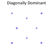
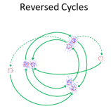
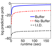
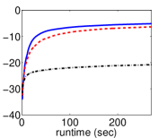
Figure 2: Synthetic experiments for DD (left) and RC (right) data. Top: Sample datasets; Arrows indicate Markov transitions. Bottom: 10-step-ahead log predictive likelihood versus learning time for DD (left) and RC (right) dynamics. Comparisons are made for SG-RLD algorithms with adaptive buffer, no buffer, and treating the data as i.i.d..

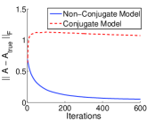
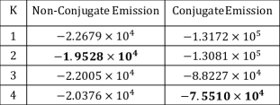
Figure 3: Synthetic experiment with log-normal emission. We use the non-conjugate emission model on the synthetic data (Top Left) with two hidden states and log-normal emissions and compare it against the conjugate model. We show the difference in convergence speed (Top Right) and log held out probability $\ln p(\mathbf{y}_{\rm test}|\mathbf{y}_{\rm train})$ on $2,000$ test data (Bottom).

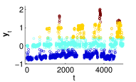
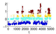
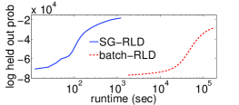
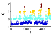
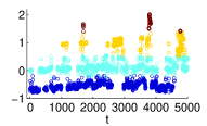
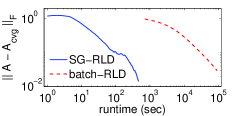
Figure 4: Inference of ion channel data Top: SG-RLD segmentation at runtimes: 44.05, 138.51, and 466.82 (sec). Bottom: Batch-RLD segmentation at runtimes: 716.19, 2124.43, and 7245.14 (sec). Right: Held-out-probability of $5000$ unobserved data points (top) and error decay of transition matrix estimates (bottom) for SG-RLD and batch-RLD methods in loglog scales. $A_{\rm cvg}$ denotes the estimated transition parameters $A$ after convergence. SG-RLD obtains plausible segmenations and accurate estimates of the transition matrix in a fraction of the time as a batch algorithm.

4.2 Non-conjugate Emission Distributions

We next demonstrate the benefit of our SG-RMCMC algorithm in being able to handle non-conjugate emissions, an essential feature to perform flexible Bayesian analyses. We simulate $2\times 10^{5}$ observations from a $2$-state HMM with log-normal emissions. Details of the parameter settings used to generate the data are in the Supplement. We evaluate the ability of two different HMM models in terms of parameter estimation and model selection accuracy.

The first HMM we consider uses log-normal emissions with non-conjugate normal priors. The second model uses Gaussian emissions with a conjugate normal-inverse-Wishart prior. In Fig. 3 we show that the non-conjugate model obtains accurate estimates of the transition matrix in substantially fewer iterations than the conjugate model. Next, we demonstrate that efficiently handling non-conjugate models leads to improved model selection. Specificallly, we use SG-RLD to fit both the conjugate and non-conjugate HMMs described above with $K=1,2,3,4$ states and compute the marginal likelihood of the observations under each model. In the table of Fig. 3 we see that the non-conjugate model selects the right number of states ($2$), whereas the conjugate model selects a model with more states ($4$). The ability to use non-conjugate HMMs for truly massive data sets has been infeasible until this point and this experiment demonstrates its utility.

4.3 Ion Channel Recordings

We investigate the behavior of the SG-RLD sampler on ion channel recording data. In particular, we consider a 1MHz recording from Rosenstein et al. (2013) of a single alamethicin channel. This data was previously investigated in Palla et al. (2014) and Tripuraneni et al. (2015) using a complicated Bayesian nonparametric HMM. In that work, the authors downsample the data by a factor of $100$ and only used $10,000$ and $2,000$ observations respectively due to the challenge of scaling computations to the full sequence. We subsample the time series by a factor of $50$, resulting in $209,634$ observations, to reduce the strong autocorrelations present in the observations that are not captured well by a vanilla HMM. However, our algorithm would have no difficulty handling the full dataset. We further log-transform and normalize the observations to use Gaussian emission.

We use a non-informative flat prior to analyze the ion channel data. In Fig. 4 we see that before the batch-RLD algorithm finishes a single iteration, the SG-RLD algorithm has already converged and generated a reasonable segmentation. With the converged estimation of the transition parameters $A$ as reference, we calculated the speed of convergence of SG-RLD and batch-RLD algorithms and found that the SG-RLD is approximately $1,000$ times faster.

5 Discussion

We have developed an SG-MCMC algorithm to perform inference in HMMs for massive observation sequences. The algorithm can be used with non-conjugate emission distributions and is thus applicable to modeling a variety of data. Also, the algorithm asymptotically samples from the true posterior as opposed to variational approaches.

Developing the algorithm relied on three ingredients. First, we derived an efficient approach to estimate the gradient of the marginal likelihood of the HMM from only small subchains. Second, we developed a principled approach using buffers to mitigate the errors introduced when breaking the dependencies at the boundaries of the subchains. Unlike previous heuristic buffering schemes, our approach is theoretically justified using random dynamical systems. Last, we utilize sampling scheme based on the mixing time of the HMM to ensure subchains are approximately independent.

In future work we will extend these ideas to other models of dependent data, such as Markov random fields. Also, the ideas presented here are not limited to MCMC and could be used to develop more principled variational inference algorithms for dependent data.

Acknowledgements

This work was supported by ONR Grant N00014-15-1-2380, NSF CAREER Award IIS-1350133, and by TerraSwarm, one of six centers of STARnet, a Semiconductor Research Corporation program sponsored by MARCO and DARPA. NF was supported by a Washington Research Foundation Innovation Postdoctoral Fellowship in Neuroengineering and Data Science.

Appendix A Gradient of the Posterior

For the hidden Markov model (HMM), the posterior distribution of all hyperparameters $\theta$ can be calculated by the Bayes rule, where

$$p(\theta|\mathbf{y})\propto p(\mathbf{y}|\theta)p(\theta).$$

Since

$$p(\mathbf{y},\mathbf{x}|\theta)=\pi_{0}(x_{0})\prod_{t=1}^{T}A_{x_{t},x_{t-1}}\cdot\prod_{t=1}^{T}p(y_{t}|x_{t}),$$

where $\mathbf{y}=(y_{1},\cdots y_{T})$ denotes the data as real valued vector, and $\mathbf{x}=(x_{1},\cdots x_{T})$ as discrete valued vector with $x_{t}\in\{1,\cdots K\},\forall t$. We can directly marginalize out the hidden variables, $\mathbf{x}$, with matrix multiplication as

$$p(\mathbf{y}|\theta)=\mathbf{1}_{T}^{\rm T}\ P(y_{T})A\cdots P(y_{1})A\ \mbox{\boldmath$\pi$}_{0},$$

where $P(y_{T})$ is a diagonal matrix and $P_{i,j}(y_{t})=p(y_{t}|x_{t}=i)\delta_{i,j}$; $\mathbf{1}_{T}^{\rm T}=(1,\cdots,1)$ is a row vector of $k$ ones (^T denotes transpose); $(\mbox{\boldmath$\pi$}_{0})_{i}=\pi_{0}(x_{0}=i)$. Hence the same as Eq. (2), (3) and (8) of the main paper, the posterior distribution is:

$$p(\theta|\mathbf{y})=\mathbf{1}_{T}^{\rm T}\ P(y_{T})A\cdots P(y_{1})A\ \mbox{\boldmath$\pi$}_{0}\cdot p(\theta).$$

When we divide the whole sequence into subsequences of

$$\mathbf{y}_{\tau,L}=(y_{\tau-L},\ldots,y_{\tau},\ldots,y_{\tau+L}),$$

the posterior can be rewritten as:

$$p(\theta|\mathbf{y})\propto\mathbf{1}^{\rm T}\prod_{\mathbf{y}_{\tau,L}\in\mathcal{S}}P(\mathbf{y}_{\tau,L})\mbox{\boldmath$\pi$}_{0}\cdot p(\theta),$$ (23)

where $\mathcal{S}$ is the minimum set of $\mathbf{y}_{\tau,L}$ covering $\mathbf{y}$.

We can then use gradient information of the posterior distribution to construct MCMC algorithms. The gradient of the log-posterior distribution is:

$$\dfrac{\partial\ln p(\theta|\mathbf{y})}{\partial\theta_{i}}=\sum_{\tau=1}^{{|\mathcal{S}|}}\dfrac{\mathbf{1}^{\rm T}P(\mathbf{y}_{{|\mathcal{S}|},L})A\cdots\dfrac{\partial\left(P(\mathbf{y}_{\tau,L})A\right)}{\partial\theta_{i}}\cdots P(\mathbf{y}_{1,L})A\mbox{\boldmath$\pi$}_{0}}{\mathbf{1}^{\rm T}P(\mathbf{y}_{{|\mathcal{S}|},L})A\cdots P(\mathbf{y}_{\tau,L})A\cdots P(\mathbf{y}_{1,L})A\mbox{\boldmath$\pi$}_{0}}+\dfrac{\partial\ln p(\theta)}{\partial\theta_{i}}.$$

Denote $\mathbf{q}_{\tau+L+1}^{\rm T}=\mathbf{1}_{T}^{\rm T}P(y_{T})A\cdots P(y_{t+1})A$ and $\mbox{\boldmath$\pi$}_{\tau-L-1}=P(y_{t-1})A\cdots P(y_{1})A\mbox{\boldmath$\pi$}_{0}$. Then

$$\dfrac{\partial U(\theta)}{\partial\theta_{i}} =-\dfrac{\partial\ln p(\mathbf{y}|\theta)}{\partial\theta_{i}}-\dfrac{\partial p(\theta)}{\partial\theta_{i}}$$

$$=-\sum_{\mathbf{y}_{\tau}\in\widetilde{\mathcal{S}}}\dfrac{\mathbf{q}_{\tau+L+1}^{\rm T}\dfrac{\partial P(\mathbf{y}_{\tau})}{\partial\theta_{i}}\mbox{\boldmath$\pi$}_{\tau-L-1}}{\mathbf{q}_{\tau+L+1}^{\rm T}P(\mathbf{y}_{\tau})\mbox{\boldmath$\pi$}_{\tau-L-1}}-\dfrac{\partial\ln p(\theta)}{\partial\theta_{i}},$$ (24)

as shown in Eq. (11) of the main paper.

Appendix B Lyapunov Exponent

The question of buffer length is equivalent to: for two random vectors $\pi$ and $\mbox{\boldmath$\pi$}^{*}$, what’s the expected length of $LB$ such that after the application of $P(\mathbf{y}_{LB})$, $\pi$ and $\mbox{\boldmath$\pi$}^{*}$ will synchronize? This is a question of random dynamical systems and can be answered through defining the Lyapunov exponent.

We first transform $\pi$ through stereographic projection into $K-1$ dimensions and denote as: $\mathbf{r}$. Then operator $P(y_{t})A[\ \cdot\ ]$ is projected to new space and the equivalent dynamics over $\mathbf{r}$ becomes: $F_{y_{t}}$. We define the Lyapunov exponent $\mathfrak{L}$ through the projected random dynamics $F_{y_{t}}$ as

$$\mathfrak{L}=\int_{\Omega\times\mathbb{R}^{K-1}}\ln||\nabla_{\mathbf{r}}F_{y}(\mathbf{r})||\textrm{d}\mu_{y}\textrm{d}\mu_{\mathbf{r}},$$ (25)

where $y\in\Omega$. Measure $\mu_{y}$ corresponds to the distribution of the data $y_{t}$, and $\mu_{\mathbf{r}}$ is the invariant measure of $\mathbf{r}$ under the dynamics of $P(y_{t})A$, which will be estimated through sampling.

Once the Lyapunov exponent $\mathfrak{L}$ is calculated, we can set the buffer length:

$$B=\dfrac{1}{\mathfrak{L}}\ln\left(\dfrac{\delta}{\delta_{0}}\right),$$ (26)

where $\delta=10^{-3}$ is the error tolerance and $\delta_{0}=2$ is the maximum initial error for probability vectors.

Appendix C Subsequence Sampling Procedure

We use the following sampling procedure to obtain the subsequences used to compute stochastic gradient estimates. In order to enforce the non-overlapping mixing-time constraint between adjacent subsequences, we sample them sequentially. This results in the following form for the probability of the minibatch $\widetilde{\mathcal{S}}$: $p(\widetilde{\mathcal{S}})=\prod_{n=0}^{R-1}L/|\mathcal{S}_{n}|$, where $|\mathcal{S}_{0}|=T$, $|\mathcal{S}_{n}|=|\mathcal{S}_{n-1}|-(\nu+2B+2L)-L_{\mathrm{overlap}}$. The quantity $L_{\mathrm{overlap}}$ is calculated as follows:

$$L_{\mathrm{overlap}}^{0}=|\tau_{n}|,$$

$$L_{\mathrm{overlap}}^{T}=|T-\tau_{n}|,$$

$$L_{\mathrm{overlap}}^{L}=\min_{n^{\prime}=1,\tau_{n^{\prime}}<\tau_{n}}^{n-1}\{|\tau_{n}-\tau_{n^{\prime}}|\}-L-B,$$

$$L_{\mathrm{overlap}}^{R}=\min_{n^{\prime}=1,\tau_{n^{\prime}}>\tau_{n}}^{n-1}\{|\tau_{n}-\tau_{n^{\prime}}|\}-L-B.$$

If $\min\{L_{\mathrm{overlap}}^{0},L_{\mathrm{overlap}}^{T},L_{\mathrm{overlap}}^{L},L_{\mathrm{overlap}}^{R}\}\geq 2\nu+3L+3B$, the minimum number of observations required to fit an entire subsequence while respecting minimum gap $\nu$, $L_{\mathrm{overlap}}=0$. Otherwise, $L_{\mathrm{overlap}}$ equals to the sum of all the above terms that are less than $2\nu+3L+3B$.

Since $T\gg L,B,\nu$, then $p(\widetilde{\mathcal{S}})$ provides the correct probability of the minibatch $\widetilde{\mathcal{S}}$.

Appendix D Detailed Descriptions of Experiments

D.1 Evaluating Buffer Effectiveness

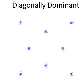
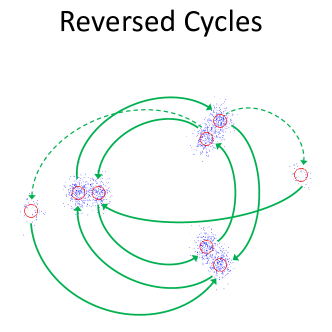
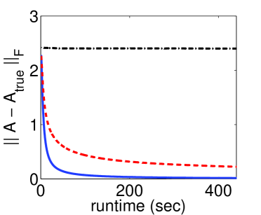
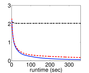
Figure 5: Synthetic experiments with hard-to-capture dynamics. Diagonally dominant (DD) (left) and reversed cycles (RC) (right) experiments. First Row: The emission distributions corresponding to $8$ different states. Arrows in the RC case indicate the Markov transition structure with transition between bridge states as dashed arrows. Second Row: Decrease of error in transition matrix estimation versus runtime. Comparisons are made for SG-RLD algorithms with estimated buffer, without buffer, and treating data as i.i.d. All of the experiments use a constant computation budget by varying the number of subchains, $|\tilde{S}|$, with the length of the subchains, $L$.

The first data set, diagonally dominant (DD) consists of a Markov chain that heavily self-transitions. Most subchains in a minibatch thus contain redundant information with observations generated from the same latent state. Although transitions are rarely observed, the emission means are set to be distinct so that this example is likelihood-dominated and highly identifiable. See Fig. 5 (top left). For this data we choose $L=2$ and $|\widetilde{S}|=10$ subsequences in order to incorporate observations from distant parts of the observation sequence. This corresponds to an extreme setting where each gradient is based only on $5$ observations. The transition matrix and emission parameters used for this experiment were:

$$A_{DD}=\left(\begin{array}[]{cccccccc}.999&.001&0&0&0&0&0&0\\ 0&.999&.001&0&0&0&0&0\\ 0&0&.999&.001&0&0&0&0\\ 0&0&0&.999&.001&0&0&0\\ 0&0&0&0&.999&.001&0&0\\ 0&0&0&0&0&.999&.001&0\\ 0&0&0&0&0&0&.999&.001\\ .001&0&0&0&0&0&0&.999\end{array}\right).$$

$$\boldsymbol{\mu}_{DD}=\left\{(0,20);(20,0);(-30,-30);(30,-30);(-20,0);(0,-20);(30,30);(-30,30);\right\}$$

and $\Sigma_{DD}=I$ for all states.

The second dataset we consider contains two reversed cycles (RC): the Markov chain strongly transitions from states $1\rightarrow 2\rightarrow 3\rightarrow 1$ and $5\rightarrow 7\rightarrow 6\rightarrow 5$ with a small probability of transiting between cycles via bridge states $4$ and $8$. See Fig. 5 (top right). The emission means for the two cycles are very similar but occur in reverse order with respect to the transitions. The emission variance is larger, making states $1$ and $5$, $2$ and $6$, $3$ and $7$ indiscernible by themselves. Transition information in observing long enough dynamics is thus crucial to identify between states $1,2,3$ and $5,6,7$. Therefore, we set $L=5$ and $|\widetilde{S}|=4$. Note that same amount of data are used in the calculation of the gradient. The transition matrix and emission parameters were:

$$A_{RC}=\left(\begin{array}[]{cccccccc}.01&0&.85&0&0&0&0&1\\ .99&.01&0&0&0&0&0&0\\ 0&.99&0&0&0&0&0&0\\ 0&0&.15&0&0&0&0&0\\ 0&0&0&1&.01&0&.85&0\\ 0&0&0&0&.99&.01&0&0\\ 0&0&0&0&0&.99&0&0\\ 0&0&0&0&0&0&.15&0\end{array}\right).$$

$$\boldsymbol{\mu}=\left\{(-50,0);(30,-30);(30,30);(-100,-10);(40,-40);(-65,0);(40,40);(100,10)\right\},$$

and $\Sigma_{RC}=20*I$ for all states.

We use a non-conjugate flat prior to demonstrate the flexibility of our algorithm. We initialize with a short run of k-means clustering to ensure that different states have different emission parameters.

D.2 Non-conjugate Emission Distribution

For the non-conjugate experiment, we used the following transition matrix:

$$\left(\begin{array}[]{cc}.1&.9\\ .9&.1\end{array}\right).$$

For emission probability, we use a log-normal distribution: $p_{k}(y)\propto e^{-\dfrac{\ln(y-\mu_{k})^{2}}{2\sigma_{k}^{2}}}$ with parameters: $\mu_{1}=0$, $\mu_{2}=4$; $\sigma_{1}=\sigma_{2}=2$.

In the non-conjugate model, we use the following priors on the emission parameters: $\mu_{1},\mu_{2},\sigma_{1},\sigma_{2}\sim\mathcal{N}(0,1)$.

References

- Amari (1998) Amari, S. Natural gradient works efficiently in learning. Neural Computation, 10(2):251–276, 1998.
- Arnold (1998) Arnold, L. Random Dynamical Systems. Springer, 1998.
- Beale (2003) Beale, M. J. Variational Algorithms for Approximate Bayesian Inference. Ph.D. thesis, University College London, 2003.
- Bishop (2006) Bishop, C. M. Pattern Recognition and Machine Learning. Springer, 2006.
- Broderick et al. (2013) Broderick, T., Boyd, N., Wibisono, A., Wilson, A. C., and Jordan, M. I. Streaming variational Bayes. In Advances in Neural Information Processing Systems, 2013.
- Bryant & Sudderth (2012) Bryant, M. and Sudderth, E. B. Truly nonparametric online variational inference for hierarchical Dirichlet processes. In Advances in Neural Information Processing Systems, 2012.
- Chen et al. (2015) Chen, C., Ding, N., and Carin, L. On the convergence of stochastic gradient mcmc algorithms with high-order integrators. In Advances in Neural Information Processing Systems 28, pp. 2278–2286. 2015.
- Chen et al. (2014) Chen, T., Fox, E. B., and Guestrin, C. Stochastic gradient Hamiltonian Monte Carlo. In Proceeding of 31st International Conference on Machine Learning (ICML’14), 2014.
- Ding et al. (2014) Ding, N., Fang, Y., Babbush, R., Chen, C., Skeel, R. D., and Neven, H. Bayesian sampling using stochastic gradient thermostats. In Advances in Neural Information Processing Systems 27 (NIPS’14). 2014.
- Foti et al. (2014) Foti, N. J., Xu, J., Laird, D., and Fox, E. B. Stochastic variational inference for hidden Markov models. In Advances in Neural Information Processing Systems, 2014.
- Fox (2009) Fox, E.B. Bayesian Nonparametric Learning of Complex Dynamical Phenomena. Ph.D. thesis, MIT, Cambridge, MA, 2009.
- Gopalan et al. (2012) Gopalan, P. K., Gerrish, S., Freedman, M., Blei, D. M., and Mimno, D. M. Scalable inference of overlapping communities. In Advances in Neural Information Processing Systems, pp. 2249–2257. 2012.
- Hoffman et al. (2013) Hoffman, M. D., Blei, D. M., Wang, C., and Paisley, J. Stochastic variational inference. Journal of Maching Learning Research, 14(1):1303–1347, May 2013.
- Hughes et al. (2015) Hughes, M. C., Stephenson, W., and Sudderth, E. B. Scalable adaptation of state complexity for nonparametric hidden Markov models. In Advances in Neural Information Processing Systems, 2015.
- Johnson & Willsky (2014) Johnson, M. J. and Willsky, A. S. Stochastic variational inference for Bayesian time series models. In International Conference on Machine Learning, 2014.
- LeGland & Mevel (1997) LeGland, F. and Mevel, L. Exponential forgetting and geometric ergodicity in hidden Markov models. In IEEE Conference on Decision and Control, 1997.
- Leimkuhler & Shang (2016) Leimkuhler, Benedict and Shang, Xiaocheng. Adaptive thermostats for noisy gradient systems. SIAM Journal on Scientific Computing, 38(2):A712–A736, 2016.
- Ma et al. (2015) Ma, Y.-A, Chen, T., and Fox, E. B. A complete recipe for stochastic gradient MCMC. In Advances in Neural Information Processing Systems 28, pp. 2899–2907. 2015.
- Ma et al. (2016) Ma, Y.-A., Fox, E. B., Chen, T., and Wu, L. A unifying framework for devising efficient and irreversible MCMC samplers. arXiv:1608.05973, 2016.
- Palla et al. (2014) Palla, K., Knowles, D. A., and Ghahramani, Z. A reversible infinite HMM using normalised random measures. In International Conference on Machine Learning, 2014.
- Patterson & Teh (2013) Patterson, S. and Teh, Y. W. Stochastic gradient Riemannian Langevin dynamics on the probability simplex. In Advances in Neural Information Processing Systems 26 (NIPS’13). 2013.
- Rabiner (1989) Rabiner, L. R. A tutorial on hidden Markov models and selected applications in speech recognition. In Proceedings of the IEEE, volume 77, pp. 257–286, 1989.
- Robbins & Monro (1951) Robbins, H. and Monro, S. A stochastic approximation method. The Annals of Mathematical Statistics, 22(3):400–407, 09 1951.
- Rosenstein et al. (2013) Rosenstein, J. K., Ramakrishnan, S., Roseman, J., and L, Shepard K. Single ion channel recordings with CMOS-anchored lipid membranes. Nano Letters, 13(6):2682–2686, 2013.
- Scott (2002) Scott, S. L. Bayesian methods for hidden Markov models: Recursive computing in the 21st century. Journal of the American Statistical Association, 97(457):337–351, 03 2002.
- Seneta (2006) Seneta, E. Non-negative matrices and Markov chains. Springer Science & Business Media, 2006.
- Shang et al. (2015) Shang, X., Zhu, Z., Leimkuhler, B., and Storkey, A. Covariance-controlled adaptive Langevin thermostat for large-scale Bayesian sampling. In Advances in Neural Information Processing Systems 28 (NIPS’15). 2015.
- Tripuraneni et al. (2015) Tripuraneni, N., Gu, S., Ge, H., and Ghahramani, Z. Particle Gibbs for infinite hidden Markov Models. In Advances in Neural Information Processing Systems, pp. 2386–2394, 2015.
- Vollmer et al. (2016) Vollmer, S. J., Zygalakis, K. C., and Teh, Y. W. Exploration of the (non-)asymptotic bias and variance of stochastic gradient Langevin dynamics. Journal of Machine Learning Research, 17(159):1–48, 2016.
- Welling & Teh (2011) Welling, M. and Teh, Y. W. Bayesian learning via stochastic gradient Langevin dynamics. In Proceedings of the 28th International Conference on Machine Learning (ICML’11), pp. 681–688, June 2011.
- (31) Ye, F. X.-F., Ma, Y.-A., and Qian, H. A numerical algorithm for calculating the rate of exponential forgetting in HMM. manuscript in preparation.