Quadratic genetic modifications: a streamlined route to
cosmological simulations with controlled merger history
Abstract
Recent work has studied the interplay between a galaxy’s history and its observable properties using “genetically modified” cosmological zoom simulations. The approach systematically generates alternative histories for a halo, while keeping its cosmological environment fixed. Applications to date altered linear properties of the initial conditions such as the mean overdensity of specified regions; we extend the formulation to include quadratic features such as local variance, which determines the overall importance of smooth accretion relative to mergers in a galaxy’s history. We introduce an efficient algorithm for this new class of modification and demonstrate its ability to control the variance of a region in a one-dimensional toy model. Outcomes of this work are two-fold: (i) a clarification of the formulation of genetic modifications and (ii) a proof of concept for quadratic modifications leading the way to a forthcoming implementation in cosmological simulations.
keywords:
methods: numerical - galaxies: formation, evolution - cosmology: dark matter1 Introduction
Mergers and accretion are thought to play a key role in shaping the observed galaxy population; in the prevailing cosmological paradigm merger histories are in turn seeded from random inflationary perturbations. Numerical studies must make inferences about the galaxy population from a finite sample of such histories. Due to the limited computer time available, this generates a tension between resolution (for resolving the interstellar medium) and volume (for adequately sampling histories).
One attempt to sidestep this problem is to create and study a small number of carefully controlled tests of the relationship between a galaxy’s history and its observable properties. This has long been attempted in idealised, non-cosmological settings (e.g. Hernquist 1993; Di Matteo et al. 2005; Hopkins et al. 2012). More recently, Roth et al. (2016) proposed performing such tests within a fully cosmological environment by constructing a series of closely-related initial conditions with targeted “genetic modifications” (hereafter GMs). The formalism resembles that of constrained realisations (Bardeen et al. 1986; Bertschinger 1987; Hoffman & Ribak 1991, hereafter HR91) which generates realisations of Gaussian random fields satisfying user-defined constraints on initial densities, velocities or potentials (e.g. Bertschinger 2001). Simulations based on constrained realisations have been extensively applied to recreating the local universe using observed galaxy distributions as constraints (for recent examples see Heß et al. 2013; Wang et al. 2016; Sorce et al. 2016; Hoffman et al. 2017).
Despite a resemblance, genetically modified simulations are markedly different from constrained simulations. The process of GM involves creating multiple versions of the initial conditions, each with carefully selected small changes. By re-simulating each scenario it becomes possible to study how the changes affect the non-linear evolution of structure. For example, modifications can be chosen such that they enhance or suppress merger ratios in incremental steps and so vary a galaxy’s history in a systematic and controlled way. The first application of this technique in a hydrodynamic simulation was made by Pontzen et al. (2017); that work focuses on the response of a galaxy’s central black hole and its ability to quench star formation as the merger history is changed gradually. Unlike studies based on fully idealised merger simulations, the GM-based approach is able to capture the effects of gradual gas accretion from filaments which is essential when probing the balance between star formation and black hole feedback.
On a technical level, Pontzen et al. (2017) used multiple linear modifications to alter the merger history. Such a method requires human effort on two fronts: (i) to identify and track particles forming the merging substructures; and (ii) to tune the modifications and understand their effects on one another. For instance, GMs suppressing a merger tend to increase the mass of other nearby substructures, which complicates interpretation of the final results (see section 2.3 and figure 2 of Pontzen et al. 2017). Bypassing this behaviour would be possible by individually identifying all substructures and demanding the algorithm fix each one. However, the spiralling complexity of the setup makes this option unattractive.
Another possibility, which is the primary aim of the present paper, is to find a new type of modification which automatically suppresses the merger ratios of all large substructures in a target galaxy’s history. Such a modification would smooth the expected history while keeping its final mass and overall environment fixed. These modifications must be applicable to cosmological simulations, so our objective is an algorithm that remains tractable even working with fields on multidimensional grids. To achieve this goal, we start by clarifying the formulation of GMs (Section 2). We then expand the framework to quadratic modifications (Section 3), allowing control over the variance at different scales to tackle the problem of multiple mergers. We demonstrate the feasibility of our method on a one-dimensional model (Section 4); in forthcoming work we will demonstrate the implementation for a full 3D zoom simulation. Results are discussed in Section 5 and we conclude in Section 6.
2 Linear constraints and modified fields
In this Section, we contrast the method of constraints (HR91) against that of linear genetic modifications. The aim is to clarify the status of the latter as a building block for non-linear GMs, which are introduced in Section 3.
2.1 Constrained ensemble
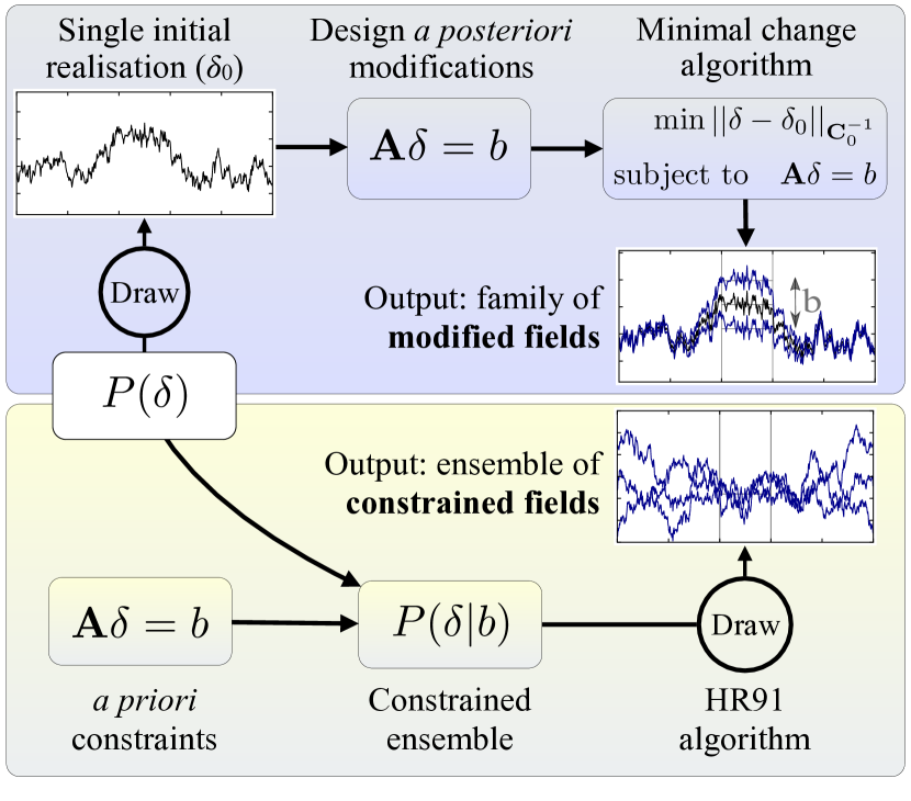
We start by reviewing the construction of constrained ensembles (see bottom panel of Figure 1). In this case, constraints must be known a priori, i.e. independently of any specific realisation. Constrained ensembles are therefore particularly useful when using observations as external inputs to constrain numerical simulations.
Consider a Gaussian random field sampled at points to create a vector with covariance matrix . The HR91 algorithm allows for an arbitrary number (denoted ) of linear constraints to be placed on ; these can be expressed as where A is a matrix and b is a length- vector.
We start by constructing the ensemble of all fields satisfying the constraint for a chosen b, i.e. . Applying Bayes’ theorem, the probability reads
| (1) |
Using the fact that is Gaussian and disregarding normalization, this relation becomes
| (2) |
where is the (-dimensional) Dirac delta function.
This expression suggests a brute force sampling solution: we could draw many trial s from the original ensemble and keep only the ones satisfying the constraints (within some tolerance). This solution is, however, computationally inefficient. Making use of the fact that the Dirac delta function can be represented as the zero-variance limit of a Gaussian, we can instead derive the following results (Bertschinger 1987):
| (3) |
where and C are the expectation and the covariance of the Gaussian distribution . By construction, all fields drawn from this distribution will satisfy the constraints ().
Hoffman & Ribak (1991) pointed out a convenient shortcut for efficiently sampling from the distribution specified by Equation (2.1). Starting from a draw of the unconstrained ensemble, , we calculate . One can then rewrite as the sum of the mean field from Equation (2.1) and a residual term , defined by:
| (4) |
From here, a draw from the constrained ensemble can be generated by recombining the residuals with the corrected mean :
| (5) |
To verify this procedure draws samples from the constrained distribution, one first writes the mapping from to in a single step:
| (6) |
Then, by calculating and , it is possible to check that the ensemble has the correct mean and covariance from Equation (2.1). The fact that is Gaussian follows from its construction as a linear transformation of . The underlying efficiency of this method is that the covariance matrix in Equation (2.1), does not depend on the value of b, allowing the term to be the same for both expressions.
In summary, the HR91 algorithm creates a draw from the constrained ensemble in two steps, using the realisation as an intermediate construction tool. It provides a computationally efficient way of generating Gaussian constrained fields.
2.2 Genetic modifications
We now turn to GMs (see upper panel of Figure 1) to constrast their formulation with that of constrained fields. The GM procedure can be summarized as follows:
-
1.
Draw the unmodified realisation .
-
2.
Define the modifications by choosing which properties of are to be modified. Unlike in the constrained field case, this is accomplished with reference to specific features of the realisation (e.g. the location and properties of particular haloes). This reflects how GMs are intended for constructing numerical experiments rather than for recreating observationally motivated scenarios. We focus first on linear modifications, i.e. of the form .
-
3.
Create the modified field (or multiple modified fields with different values of b). We require changes between fields to be as small as possible, which relies on the definition of a distance in field space. In the context of Gaussian fields, the only available metric is defined by the distance,
(7)
Consequently, GMs can be formulated as finding the modified field solution of the following optimization problem:
| (8) |
The problem is solved by minimising the Lagrangian
| (9) |
where is a vector of size containing the Lagrange multipliers for each modification.
By differentiating to find critical points with respect to and , we obtain a system of two vector equations with the solution
| (10) |
where is the modified field.
Equation (10) has regenerated Equation (6) using a different motivation and derivation. To summarise:
- •
- •
- •
GMs should therefore be seen as a mapping between fields of the same ensemble. A family of modified fields is generated by choosing multiple values for b; the resulting mapping between members of the family is continuous and invertible. These properties are highly valuable for providing controlled tests, allowing for systematic exploration of the effects of formation history on a galaxy.
While the algorithm makes the minimal changes to the field, may still not be a particularly likely draw from if the modifications are too extreme. To quantify the level of alteration, the relative likelihood of the two fields is given by with
| (11) |
As long as stays small, we can regard the modified and unmodified fields as similarly likely draws from initial conditions.
Turning into a precise quantitative statement about the relative abundance of a particular galactic history remains a topic for future research. It relies on knowing the detailed Jacobian relating the initial conditions to properties of the final galaxy. This can so far only be estimated, and only in simple scenarios such as small modifications to the halo mass (Roth et al., 2016). There are multiple possible modifications (i.e. choices of A and b) leading to a given effect in the target galaxy history (Porciani, 2016); some will carry a smaller cost than others. Finding the minimum-cost route to a given change in the non-linear universe is not the aim of GMs; to perform galaxy formation experiments, we only need to find one choice of modification with an acceptably small penalty.
3 Extension to quadratic modifications
The main aim of this paper is to formulate modifications that control the variance of a field. The variance on scales smaller than the parent halo scale relates to the number of substructures in haloes (Press & Schechter 1974; Bond et al. 1991), and is therefore a proxy for the overall importance of mergers. It is important to distinguish variance modifications of a region from alterations to the power spectrum. The power spectrum defines only the average variance over the entire box, and over all possible realisations. We propose on the other hand to modify the local variance, targeting one region of interest and making minimal changes to the remaining structures. Another way to picture this goal is as follows. In any one stochastic ensemble, two realisations might by chance have enhanced or reduced variance in an area. Our procedure aims to map between such realisations rather than to modify the underlying power spectrum.
Variance is quadratic in the field value and therefore the approach in Section 2.2 cannot be applied directly. One natural formulation of the problem is through a new minimisation problem (analogous to the original linear case):
| (12) |
where Q is a matrix and is a scalar. We can assume without loss of generality that Q is Hermitian. For a suitable choice of Q (see Section 4), specifies the variance of a chosen region.
Following a similar approach to the linear modifications, we introduce the Lagrangian
| (13) |
where is a scalar Lagrange multiplier associated with the quadratic modification. Searching for critical points, we obtain two equations relating the modified field and the multiplier:
| (14) | |||
| (15) |
Equation (14) and (15) provide a closed system for and given a target . Unlike the linear case, the system can not be solved analytically. A possibility would be to solve Equation (15) numerically for but direct matrix inversions are prohibited due to their computational cost. One would therefore need to perform approximate matrix inversion at each step of a root-finding scheme for , making the worst-case complexity of such method infeasible.
There are moreover deeper reasons why such procedures can not be straightforwardly adapted to GMs. In the linear case discussed above, we defined GMs as a continuous and invertible mapping. Both of these properties are lost when looking at Equations (14) and (15). First, it is not clear that Equation (15) has a real solution for . Consequently a real-valued may not exist111We note in passing that, since variance is a positive quantity, Q is a positive semi-definite matrix. By definition, is positive definite. These conditions ensure that is unique if it exists – but they do not guarantee existence. for any chosen value of .
Second, the relationship between and is asymmetric: if a new field is constructed by taking back to its original value , we will have
| (16) |
for suitable choices of and . To obtain a solution allowing recovery of the initial field (), it must hold that . This will not generally be the case for our applications, and so we conclude that in general . Such asymmetry would be problematic for GM; the sense of a unique ‘family’ of fields is lost.
The combination of computational intractability and loss of key properties for GMs lead us to focus on an alternate method. We describe next a Newton-like method which efficiently approximates a solution to the optimization problem, Equation (12), while reinstating the desired properties of the GM mapping.
3.1 Linearised solution
In this section, we restate the quadratic problem in a way that has a guaranteed solution and that generates a single family as a function of . The trick is to make only infinitesimally small changes to the value of , building up finite changes by following a path through field space that is locally minimal. This leads to an iterative procedure for quadratic genetic modifications, which we will demonstrate is both unique and computationally tractable.
3.1.1 One infinitesimal step
We start by defining the displacement from the unmodified field ; for sufficiently small changes we may then neglect terms. We will discuss in Section 3.1.3 how to practically decompose a macroscopic change into a series of such minor modifications.
At first order, the updated variance (or other quadratic property) is given by
| (17) |
where we have assumed is real and made use of the previously stated Hermitian assumption, . Having linearised the modification, we can now find an analytic solution for the displacement and the multiplier :
| (18) | ||||
| (19) |
Equation (19) does not involve matrix inversions and can therefore be efficiently evaluated, even in a 3D cosmological simulation context.
3.1.2 Building finite changes by successive infinitesimal updates
We now want to construct a macroscopic change in the field by iterating the infinitesimal steps of Equation (18). Performing a finite number of steps , the modified field reads:
| (20) |
where is the Lagrange multiplier at step . The value of each depends on how the fixed interval is divided, i.e. implicitly on . In the limit of increasing number of steps, each individual becomes infinitesimally small and the final solution is
| (21) |
where is the overall displacement and is finite. The right-hand side of Equation (21) defines the matrix exponential operator, which is guaranteed to exist and is invertible.
The matrix exponential is a useful formal expression to show that there is a unique result, but does not help computationally since the required value of to reach the objective is unknown. In practice, we use the finite approximation, Equation (20). The at each step are chosen by targeting intermediate modifications linearly spaced between the starting value and the target . At each step, is calculated using Equation (19); is deduced with Equation (18); and the field is updated, .
3.1.3 Step choice for a practical algorithm
When calculating Equation (20) as an approximation to Equation (21), the accuracy will increase with the number of steps . One must choose a minimal (for computational efficiency) while ensuring that linearly approximating the modification at each step is sufficiently accurate.
We first perform the calculation with a fixed number of steps . This gives rise to an initial estimate for the modified field that we denote . The error on the resulting modification can be characterised by the magnitude of , where
| (22) |
Because second-order terms are neglected in the modification, the error term should scale inverse-quadratically with the number of steps . We verified this behaviour numerically for a variety of fields and modifications. If is smaller than a desired precision, , we retain the initial estimate as our final output field. Otherwise, the calculation must be repeated; the required number of steps to achieve the target precision is inferred from the quadratic scaling as
| (23) |
Note that should be kept small to avoid unnecessary iterations; has been chosen for our test scenarios below.
The final algorithm has a worst-case complexity of , where is the number of elements in the field . The arises from matrix multiplications required to compute each step; in practice the matrices will be sparse either in Fourier space (for the covariance matrix) or in real space (for the variance Q matrix). Therefore, one can speed up the matrix multiplications by transforming back and forth from real to Fourier space, improving the complexity to .
The final procedure shares numerous similarities with Newton methods, used in large-scale optimization (see Nocedal & Wright 2006 for a comprehensive review). It retains quadratic information in the objective and linear information in the modification at each step and has a quadratic rate of convergence to the solution.
3.2 Joint quadratic and linear modifications
The algorithm above can be generalised to the case where we have both a quadratic modification and linear modifications of the form . We first apply the linear modifications using Equation (8), then turn to the iterative quadratic modifications. However if Equation (20) is applied directly, the linear objective will no longer be satisfied; in other words we need to enforce at each step. Constructing and solving the appropriate minimisation, expression (18) is replaced by
| (24) |
where
| (25) |
These results can be iterated to achieve the final modified field, in exactly the same way as for the pure-quadratic modification.
Despite the complexity of these expressions, the evaluation will remain for reasons discussed previously. To help interpret the method, there is a clear geometric meaning for each term, which we present in Appendix B.
4 Demonstration
In this Section we demonstrate our algorithm in a -pixel, one-dimensional setting as a proof of concept and as a reference for future implementation on cosmological simulations. We choose an example red power spectrum, as typically encountered on the scales from which galaxies collapse. Specifically, we adopt , where is an arbitrary normalisation and , an offset that prevents divergence of at .
4.1 Defining an example modification
The framework developed in Section 3 can alter any property that is quadratic in the field by suitable choice of Q. We now specialise to the case that Q corresponds to the variance of a length- region of the field. We start by defining the windowing operator W as a rectangular matrix picking out the desired entries from the pixels in . To calculate the variance of the region, one then calculates where can be written
| (26) |
Here, I is the identity matrix and 1 is a length- vector of ones. Expression (26) is readily verified by constructing and seeing that it does boil down to the variance of the chosen region.
We wish to consider the field variance only on scales smaller than the region size (corresponding to substructures with mass lower than that of the parent halo). To achieve this, can be high-pass filtered; we use a standard Gaussian high-pass filter F where in Fourier space the elements of are given by
| (27) |
Here, is the wavenumber of the -th Fourier series element and , the filtering scale, is defined in our case by . The most appropriate choice of filtering scales and shapes in the context of cosmological simulations will be discussed in a forthcoming paper.
In real space the matrix F is defined by where U is the unitary Fourier transform matrix. Finally, to localise the target modification fully, we can re-window the matrix after smoothing. The operator achieves this by setting pixels outside the target window to zero. With this set of choices, the final quadratic objective is set by
| Q | ||||
| (28) |
In practice, we never calculate the matrix Q explicitly but rather implement a routine to efficiently calculate for any field , which is then used by the algorithm described in Section 3. The ability to bypass storing or manipulating Q is essential to permit the computation to operate on a 3D cosmological simulation.
4.2 Results
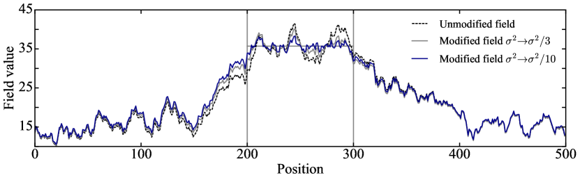
Figure 2 shows examples of modified fields obtained with our algorithm. We alter the variance of a region of width pixels enclosed by vertical lines, showing two quadratic modifications with the variance reduced by a factor 3 (light grey) and a factor 10 (dark blue). In both cases, the mean of the field is held fixed at the unmodified value (horizontal line). In the setting of a cosmological simulation, we expect to be able to fix the parent halo mass (through the mean value) while modifying the smoothness of accretion (through the variance).
We verified that these fields achieve the linear modification to within numerical accuracy and the quadratic modification to accuracy. The heights of small-scale peaks inside the enclosed region are successfully reduced and brought closer to the mean value for the modified fields. Visually, it can be seen that the changes to the field are minimal, maintaining as much as possible of the structure of the unmodified field in the modified versions. This underlines how the analytic minimisation, Equation (12), and its refinement to a linearised procedure (Section 3.1) agrees with the intuitive sense of making minimal changes. The different versions of the field form a continuous family as illustrated by the smooth deformation when reducing the variance by different factors.
Despite the modification objective Q being strictly confined to the target region, modifications can be seen to “leak” outside (beyond the vertical lines). This effect, which is also seen in linear GMs, is an intentional aspect of the minimisation construction – any sharp discontinuities in the field value or its gradients would give rise to a power spectrum inconsistent with the ensemble. In this specific example, the leakage appears more significant to the left than to the right of the target region. In general, the algorithm is spatially symmetric but its effect in any given case is not.
5 Discussion
5.1 The advantage of quadratic over linear modifications
Pontzen et al. (2017) showed that using multiple linear modifications was sufficient to change the merger ratios in the history of a galaxy; substructures can be diminished or enhanced by manually modifying individual peak heights.
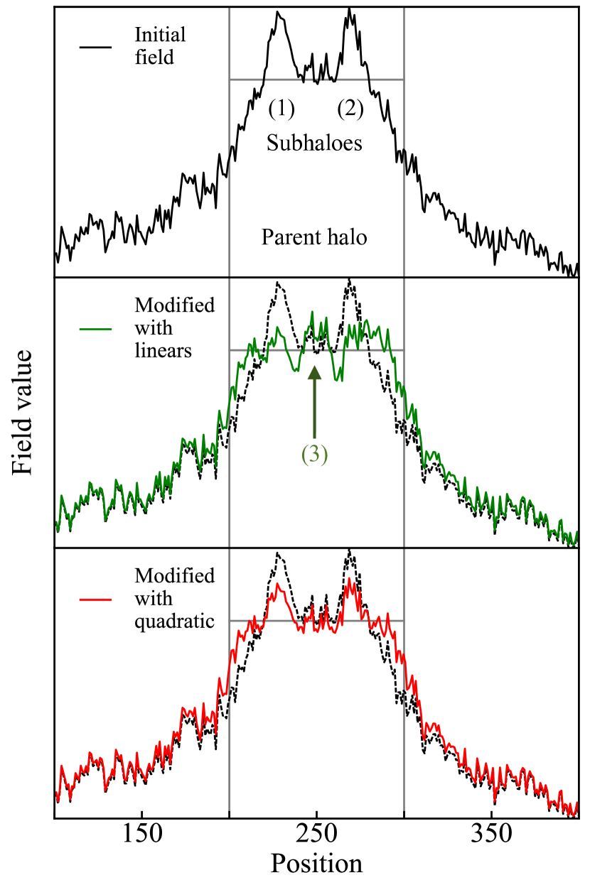
Nonetheless, we expect the new quadratic approach to bring considerable benefits when making such manipulations; the advantages are illustrated in Figure 3. The top panel shows a field representing the density in initial conditions expected for a halo. The field has a broad overdensity enclosed by vertical lines and two narrower peaks labelled (1) and (2). According to the excursion-set formalism (Bond et al., 1991), (1) and (2) will collapse to form two separate haloes that later merge. This, together with smooth accretion, will form the final halo.
Suppose we wish to generate a smoother accretion history by reducing the heights of peaks (1) and (2) while maintaining the large-scale overdensity. In the original approach, we use linear GMs to set the mean values of the peaks to the mean value of the broad overdensity (horizontal line). The middle panel of Figure 3 presents the resulting field. However, a number of problems arise when performing the alteration using this approach.
-
1.
We had to identify (1) and (2) as the most interesting substructures and define specific modifications for each. In the context of N-body simulations, this requires manually identifying which particles of the initial conditions constitute each individual subhalo.
-
2.
More importantly, spatially neighbouring modifications interact and create new substructures (peak labelled (3) in our example). One solution to prevent the appearance of new substructures could be to add a new linear objective forcing problematic regions such as (3) to remain unmodified. Identifying and mitigating side effects in this way adds a layer of complexity to the linear GM procedure. Depending on the specific problem and the number of modifications at play, time spent at this tuning phase can rise steeply.
On the other hand, a single quadratic modification can avoid these problems by defining a variance target across the region. The third panel of Figure 3 shows the same field with variance reduced by a factor 10 (using the method from Section 4). The two local peaks are successfully reduced in amplitude while conserving the remaining small-scale structure of the parent halo. By construction, the variance modification naturally avoids compensation problems inherent to linear GMs. For this reason, quadratic GMs provide a cleaner, streamlined way to control merger histories.
5.2 Multiple quadratic modifications
The formalism discussed so far applies a single quadratic modification to a field (possibly in combination with linear objectives). Simultaneously applying multiple quadratic modifications would allow one to act concurrently on two separate haloes, or to further fine-tune the merger history of a single object. For instance, decreasing the variance on intermediate scales while increasing on small scales should increase the frequency of minor mergers.
To study this generalisation, we introduce quadratic modifications, each with matrix . For an infinitesimal update, the change in the field is then given by
| (29) | ||||
| (30) |
where are the Lagrange multipliers associated with each modification. Equation (30) defines a system of equations to be solved. The resulting value of a specific depends on the whole set of and , i.e. modifications are interdependent.
In the same way as Section 3.1, the update (29) can be iterated to create finite changes. Performing steps, the modified field reads
| (31) |
where is the multiplier at step . However in the limit that the number of steps , convergence to the matrix exponential,
| (32) |
is only guaranteed if either the commute with respect to (i.e. ) or each is directly proportional to . Because s are not known in advance, the latter option is hard to arrange; the previously noted interdependence of the s on all and exacerbates the difficulty.
With our current algorithms, convergence to the matrix exponential is therefore only assured when the matrices commute. The easiest way to arrange for the commutation is to use orthogonal modifications, i.e.
| (33) |
Physically, this requirement can be achieved by imposing modifications that are spatially separated by a sufficient number of correlation lengths or address distinct Fourier modes. This condition even allows one to apply the formalism of Section 3.1 to each modification one-by-one and still converge to the correct overall matrix exponential of Equation (32). We leave the case of non-orthogonal multiple quadratic modifications to further work.
6 Conclusions
We have presented an efficient algorithm to modify the variance in a particular region of a Gaussian random field realisation, with the aim of manipulating initial conditions for cosmological simulations. The modification produces a field that is as close as possible to the original realisation. In this way it provides a route for controlled tests of galaxy formation where multiple versions of the same galaxy are simulated within a fixed cosmological environment, but with altered accretion history.
We argued that quadratic controls, as developed here, offer a useful complement to the existing linear technique (Roth et al., 2016). In particular, variance on different filtering scales relates to dark matter halo substructure and merging history (Press & Schechter 1974; Bond et al. 1991). The new algorithm can construct GM fields with simultaneous control on the mean value and filtered variance of a region (Figure 2). This provides a route to altering merger history and accretion over the lifetime of a given halo in a way that is more streamlined than modifying individual substructures (see Figure 3).
In both linear and quadratic GM, the algorithm searches for fields which are nearby in the sense of the distance measure. In the quadratic case, this definition is further refined: for large shifts in the control parameter (which represents the variance in our test cases), the path through field space is defined by following a series of small shifts. Each of these individually minimize the distance travelled. We demonstrated a formal convergence property for this series and argued that the approach is desirable for (a) returning a continuously-deforming field as a function of the changing target variance ; (b) being reversible, so that returning the variance to its initial value also returns the field to its initial state; (c) being numerically tractable even for 3D zoom simulations.
In the process, we clarified the mathematical formulation of GM, carefully distinguishing it from the constrained ensemble of HR91 (see Figure 1 for an overview). The status of fields constructed in the two approaches is distinct – unlike constrained realisations, GMs should be seen as a mapping between two fields from the same ensemble. In the case of quadratic objectives such as variance, even the cosmetic similarities between constraints and modifications are lost (Appendix A).
The next step is an implementation of the new algorithm in a full -body initial conditions generator, including on varying-resolution grids appropriate to zoom simulations. This will be presented in a forthcoming paper where we will evaluate the effectiveness of quadratic GM (alongside the existing linear technique) for constructing controlled tests of galaxy formation.
Acknowledgements
We thank Amélie Saintonge for helpful discussions and Hiranya Peiris for useful comments on a draft manuscript. MR acknowledges supports from the Perren Fund and the IMPACT fund. AP is supported by the Royal Society.
References
- Bardeen et al. (1986) Bardeen J. M., Bond J. R., Kaiser N., Szalay A. S., 1986, ApJ, 304, 15
- Bertschinger (1987) Bertschinger E., 1987, ApJ, 323, L103
- Bertschinger (2001) Bertschinger E., 2001, ApJS, 137, 1
- Bond et al. (1991) Bond J. R., Cole S., Efstathiou G., Kaiser N., 1991, ApJ, 379, 440
- Di Matteo et al. (2005) Di Matteo T., Springel V., Hernquist L., 2005, Nature, 433, 604
- Hernquist (1993) Hernquist L., 1993, ApJS, 86, 389
- Heß et al. (2013) Heß S., Kitaura F.-S., Gottlöber S., 2013, MNRAS, 435, 2065
- Hoffman & Ribak (1991) Hoffman Y., Ribak E., 1991, ApJ, 380, L5
- Hoffman et al. (2017) Hoffman Y., Pomarède D., Tully R. B., Courtois H. M., 2017, Nature Astronomy, 1, 0036
- Hopkins et al. (2012) Hopkins P. F., Kereš D., Murray N., Quataert E., Hernquist L., 2012, MNRAS, 427, 968
- Nocedal & Wright (2006) Nocedal J., Wright S. J., 2006, Numerical Optimization, 2nd edn. Springer
- Pontzen et al. (2017) Pontzen A., Tremmel M., Roth N., Peiris H. V., Saintonge A., Volonteri M., Quinn T., Governato F., 2017, MNRAS, 465, 547
- Porciani (2016) Porciani C., 2016, MNRAS, 463, 4068
- Press & Schechter (1974) Press W. H., Schechter P., 1974, ApJ, 187, 425
- Roth et al. (2016) Roth N., Pontzen A., Peiris H. V., 2016, MNRAS, 455, 974
- Sorce et al. (2016) Sorce J. G., et al., 2016, MNRAS, 455, 2078
- Wang et al. (2016) Wang H., et al., 2016, ApJ, 831, 164
Appendix A Constructing constrained ensembles for quadratic constraints
In Section 2, we contrasted the notion of a linearly-constrained ensemble (Section 2.1) against that of genetic modifications (Section 2.2). While conceptually different, constrained ensembles can be sampled using the HR91 procedure which can in turn be seen as applying suitable modifications to realisations from the unconstrained pdf.
In this Appendix we show that there is no such similarity between quadratically-constrained ensembles and quadratically modified fields. To put it another way, there is no HR91-like method for generating samples from a quadratically-constrained ensemble.
Following the same Bayesian argument as in Section 2.1, we define the quadratically-constrained ensemble for a fixed Q and by
| (34) |
We will show that the modification procedure does not generate samples from the ensemble (34), even when Q and are known and fixed in advance.
We start by defining the alternative ensemble to be that sampled by drawing an unconstrained field from and using the GM procedure to enforce the constraint . In Section 3.1, the mapping was given by
| (35) |
where is the covariance matrix of the Gaussian distribution and the value of is implicitly defined by the need to satisfy the quadratic constraint .
To incorporate this implicit requirement to choose the correct value of into an expression for the ensemble, we make use of Bayes’ theorem:
| (36) |
Note that the constraint demands , where and are related by the condition (35). Writing out the normalisation condition for then gives
| (37) |
Because Q and are positive semi-definite, is a monotonically increasing function of ; there is only one value of which satisfies the Dirac delta function on the right-hand-side. Consequently, we can perform the integration by a change of variables to yield
| (38) |
Substituting this result back into Equation (36) and performing the integral over using , one obtains
| (39) |
where normalisation factors depending only on have been dropped. This expression no longer has any explicit reference to , which was our primary aim. It can now be compared with the distribution for a true constrained ensemble, Equation (34). The two distributions appear different (as expected given our claim of inequivalence), but the comparison is complicated by the unsolved integral over which obscures the content of the expression.
We can see that this integral will never regenerate the true quadratic constrained ensemble by taking an illustrative example. Consider a three-dimensional field with unit power spectrum (). Let us further choose an explicit form for Q such that
| (40) |
Inserting these results into Equation (39) gives
| (41) | ||||
where we have made the substitution . The integral over has an analytical solution using the further substitution and introducing the modified Bessel function of the second kind
| (42) |
Equation (39) can then be evaluated explicitly to obtain
| (43) |
For comparison, the quadratic constrained ensemble in this example is given by
| (44) |
The distributions defined by (43) and (44) have identical -dependence. This is a general property: degrees of freedom for which Q has a null direction are unconstrained and, similarly, left unchanged by our GM transformation. The distribution generated by these degrees of freedom will therefore coincide at all times with the constrained ensemble. However, the and dependences differ between Equations (43) and (44). In general, non-null directions in field space will behave differently between the GM and constrained ensemble cases.
The result establishes that our formulation of quadratic GM as a matrix exponential mapping does not reproduce a quadratically-constrained ensemble when used analogously to the HR91 algorithm. A similar argument allows one to verify that applying the alternative non-linear modification specified by Equation (14) also fails to regenerate the constrained result. In fact, one can go even further and write a general power series expansion for the mapping between and , writing
| (45) |
without further specifying the power series coefficients . Even in this case, which generalises away from a specific mapping, it is not possible to generate a constrained ensemble from the modification procedure. This underlines that modifications and constraints need to be regarded as entirely separate procedures. Only in the linear case do they appear to be cosmetically related.
Appendix B Geometrical interpretation
Throughout the main text, we used fields sampled at a finite number of points ; the resulting algorithms can therefore be interpreted geometrically as acting on vectors in an -dimensional space. For instance, Roth et al. (2016) noted that the linear GM procedure is equivalent to an orthonormal projection of the unmodified field onto a subspace defining the modification objective (see their appendix A). In this Appendix we provide the geometric interpretation for our extended formulation of GM.
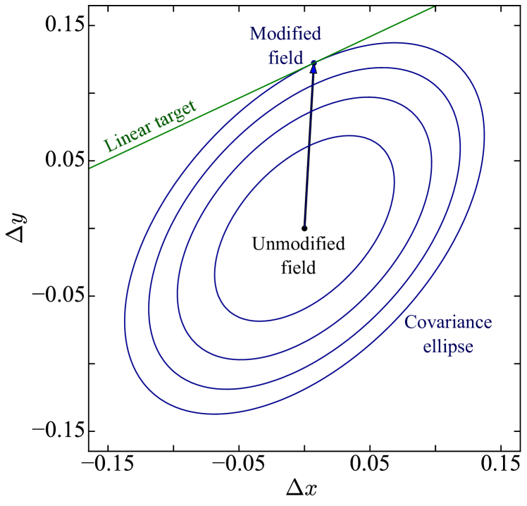
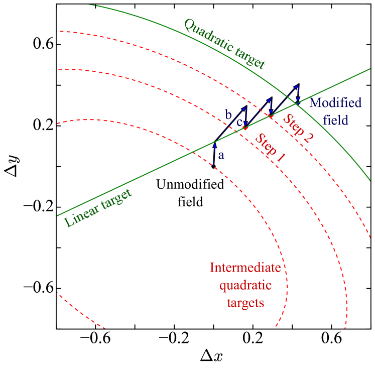
For the purposes of visualising the connection, we use fields with only two samples, . The arguments of this Appendix generalise to higher dimensions but are easiest to visualise with . Figure 4 shows the resulting two-dimensional geometry in terms of the displacements and from the unmodified field. By construction, the unmodified field is at the origin.
The left panel shows the elliptical geometry generated by the covariance matrix in the – plane; specifically, the ellipses are of constant distance from the origin, where
| (46) |
The linear objective defines a line in two dimensions. The modification consists of finding the value of lying on the line, while minimising . Since is measured in terms of , the solution does not correspond to the closest point on the page but to the point at which a covariance ellipse is tangent to the modification line.
Similarly, the quadratic modifications (right panel of Figure 4) are associated with ellipses of constant . These targets are shown as dotted lines; note that they are centred on and therefore appear offset from the origin in the – plane.
The right panel of Figure 4 also illustrates the algorithm for finding the modified field with a simultaneous quadratic and linear objective. For visual clarity, an unrealistically small () number of steps are taken. We start by defining three intermediate ellipses (red-dotted) between the value of the modification at the unmodified field and the target. As explained in Section 3.2, we first apply the global linear modifications from Equation (8)
| (47) |
The algorithm then iterates the step defined by Equation (24)
| (48) |
These operations can be understood geometrically as:
-
(a) A projection of the current field on the linear modification. This term is similar to the case with linear modifications only.
-
(b) A displacement along the normal of the ellipse at the current field value. This term is towards the next intermediate ellipse.
-
(c) The projection of the previous term back onto the linear modification to ensure that both are always satisfied.
Term (c) ensures that the current field at the end of each step always lies on the linear constraint. Term (a) therefore vanishes after the first step; it is an overall offset that needs to be applied only once. Together, (b) and (c) are locally orthogonalizing the quadratic modification with respect to the global linear modification. The orthogonalisation must be repeated at each step since the local linearisation changes as we progress towards the final value of .