Upper bounds on secret key agreement over lossy thermal bosonic channels

Abstract

Upper bounds on the secret-key-agreement capacity of a quantum channel serve as a way to assess the performance of practical quantum-key-distribution protocols conducted over that channel. In particular, if a protocol employs a quantum repeater, achieving secret-key rates exceeding these upper bounds is a witness to having a working quantum repeater. In this paper, we extend a recent advance [Liuzzo-Scorpo et al., Phys. Rev. Lett. 119, 120503 (2017)] in the theory of the teleportation simulation of single-mode phase-insensitive Gaussian channels such that it now applies to the relative entropy of entanglement measure. As a consequence of this extension, we find tighter upper bounds on the non-asymptotic secret-key-agreement capacity of the lossy thermal bosonic channel than were previously known. The lossy thermal bosonic channel serves as a more realistic model of communication than the pure-loss bosonic channel, because it can model the effects of eavesdropper tampering and imperfect detectors. An implication of our result is that the previously known upper bounds on the secret-key-agreement capacity of the thermal channel are too pessimistic for the practical finite-size regime in which the channel is used a finite number of times, and so it should now be somewhat easier to witness a working quantum repeater when using secret-key-agreement capacity upper bounds as a benchmark.

year number number identifier LABEL:FirstPage1 LABEL:LastPage#1102

I Introduction

One of the main goals of quantum information theory H13book ; H06 ; W15book  is to establish bounds on communication rates for various information-processing tasks. An important application lies in the domain of secret communication, following the development of quantum key distribution bb84 ; E91 . In recent years, there has been a growing interest in establishing bounds on the secret-key-agreement capacity of a quantum channel, which is the highest rate at which communicating parties can use the channel and public classical communication to distill a secret key TGW14IEEE ; TGW14Nat ; STW16 ; PLOB15 ; Goodenough2015 ; TSW16 ; AML16 ; WTB16 ; Christandl2017 ; Wilde2016 ; BA17 ; RGRKVRHWE17 ; TSW17 . Such bounds have been proven by exploiting the methods of quantum information theory and can be interpreted as setting the fundamental limitations of quantum key distribution whenever a quantum repeater is not available L15 .

An important development occurred in TGW14Nat , in which it was established that there is a fundamental rate-loss trade-off that any repeaterless quantum key distribution protocol cannot overcome. That is, without a quantum repeater, the rate of secret key that can be distilled from a pure-loss bosonic channel (lossy optical fiber or a free-space channel) decreases exponentially with increasing distance TGW14Nat .

Later, this bound was improved to establish that the secret-key-agreement capacity of a pure-loss bosonic channel of transmissivity $\eta\in(0,1)$ is equal to $-\log_{2}(1-\eta)$. This bound was claimed in PLOB15 and rigorously proven in WTB16 . In particular, let $P_{\mathcal{L}_{\eta}}^{\leftrightarrow}(n,\varepsilon)$ denote the highest rate at which $\varepsilon$-close-to-ideal secret key can be distilled by making $n$ invocations of a pure-loss channel $\mathcal{L}_{\eta}$ of transmissivity $\eta$, along with the assistance of public classical communication WTB16 . In WTB16 , $P_{\mathcal{L}_{\eta}}^{\leftrightarrow}(n,\varepsilon)$ is called the non-asymptotic secret-key-agreement capacity of the channel $\mathcal{L}_{\eta}$. One of the results of WTB16 is the following fundamental upper bound:

$$P_{\mathcal{L}_{\eta}}^{\leftrightarrow}(n,\varepsilon)\leq-\log_{2}(1-\eta)+\frac{C(\varepsilon)}{n},$$ (1)

where $C(\varepsilon)=\log_{2}6+2\log_{2}(\left[1+\varepsilon\right]/\left[1-\varepsilon\right])$. The bound in (1) is known as a strong converse bound because it converges to the secret-key-agreement capacity $-\log_{2}(1-\eta)$ in the limit as $n\rightarrow\infty$. We suspect that there is little room for improvement of the bound in (1) and discuss this point further in Appendix A. The bound in (1) is to be contrasted with the following weak-converse bound:

$$P_{\mathcal{L}_{\eta}}^{\leftrightarrow}(n,\varepsilon)\leq\frac{1}{1-\varepsilon}\left[-\log_{2}(1-\eta)+\frac{h_{2}(\varepsilon)}{n}\right],$$ (2)

which follows as a direct consequence of (WTB16, , Section 8) and (WR12, , Eq. (2)) (see also (MW12, , Eq. (134))). For the benefit of the reader, we explain how to arrive at this weak-converse bound in more detail in Appendix B. In the above,

$$h_{2}(\varepsilon)=-\varepsilon\log_{2}\varepsilon-(1-\varepsilon)\log_{2}(1-\varepsilon)$$ (3)

denotes the binary entropy. The bound in (2) is a weak-converse bound because it requires the extra limit as $\varepsilon\rightarrow 0$ after taking the limit as $n\rightarrow\infty$, in order to arrive at the capacity upper bound of $-\log_{2}(1-\eta)$. The significance of the bounds in (1) and (2) is that they apply for any finite number $n$ of channel uses and key-quality parameter$~{}\varepsilon$. As such, these bounds can be used to assess the performance of any practical secret-key-agreement protocol conducted over a pure-loss channel$~{}\mathcal{L}_{\eta}$.

The pure-loss channel is somewhat of an ideal model for a communication channel, even if it does have a strong physical underpinning in the context of free-space communication YS78 ; S09 . In particular, a working assumption of the model is that the channel input interacts with an environment prepared in the vacuum state. However, in practical setups, we might expect the environment to be modeled as a thermal state of a fixed mean photon number $N_{B}>0$ S09 , and in such a case, the channel is called a thermal channel and denoted by $\mathcal{L}_{\eta,N_{B}}$ (also called thermal-lossy channel, as in RGRKVRHWE17 ). This added thermal noise is often called excess noise NH04 ; LDTG05 , which can serve as a simple model of tampering by an eavesdropper. Additionally, there are realistic effects in communication schemes, such as dark counts of photon detectors that can be modeled as arising from thermal photons in the environment S09 ; RGRKVRHWE17 . As such, it is an important goal to establish upper bounds on the secret-key-agreement capacity of the thermal channel in order to assess the performance of practical secret-key-agreement protocols, and the main contribution of the present paper is to establish upper bounds on the non-asymptotic secret-key-agreement capacity $P_{\mathcal{L}_{\eta,N_{B}}}^{\leftrightarrow}(n,\varepsilon)$ of the thermal channel $\mathcal{L}_{\eta,N_{B}}$, which improve upon the prior known bounds from PLOB15 ; WTB16  in certain regimes.

Prior works established that

$$-\log_{2}(\left[1-\eta\right]\eta^{N_{B}})-g(N_{B})$$ (4)

is an upper bound on the secret-key-agreement capacity of a thermal channel $\mathcal{L}_{\eta,N_{B}}$ with transmissivity $\eta\in(0,1)$ and thermal mean photon number $N_{B}>0$. This bound was claimed in PLOB15 and rigorously proven in WTB16 . In this expression,

$$g(N_{B})=(N_{B}+1)\log_{2}(N_{B}+1)-N_{B}\log_{2}N_{B}$$ (5)

is the entropy of a thermal state of mean photon number $N_{B}$. In particular, the following bound was given in (WTB16, , Section 8)

$$P_{\mathcal{L}_{\eta,N_{B}}}^{\leftrightarrow}(n,\varepsilon)\leq-\log_{2}(\left[1-\eta\right]\eta^{N_{B}})-g(N_{B})\\ +\sqrt{\frac{2V_{\eta,N_{B}}}{n\left(1-\varepsilon\right)}}+\frac{C(\varepsilon)}{n},$$ (6)

where

$$V_{\eta,N_{B}}=N_{B}(N_{B}+1)\log_{2}^{2}(\eta\left[N_{B}+1\right]/N_{B}),$$ (7)

and the following weak-converse bound is a direct consequence of (WTB16, , Section 8) and WR12 ; MW12 (explained also in Appendix B):

$$P_{\mathcal{L}_{\eta,N_{B}}}^{\leftrightarrow}(n,\varepsilon)\leq\\ \frac{1}{1-\varepsilon}\left[-\log_{2}(\left[1-\eta\right]\eta^{N_{B}})-g(N_{B})+\frac{h_{2}(\varepsilon)}{n}\right].$$ (8)

Again, the value of these bounds is that they apply for any finite number $n$ of channel uses and key-quality parameter $\varepsilon$. However, by inspecting (6), we see that the order $1/\sqrt{n}$ and lower terms are strictly positive.

The main contribution of the present paper is to improve the bound in (6) in such a way that the order $1/\sqrt{n}$ term is negative whenever $\varepsilon<1/2$, representing the backoff from capacity incurred by using the channel a finite number of times while allowing for non-zero error. In fact, we find the following improved bound for several realistic values of $\eta$ and $N_{B}$:

$$P_{\mathcal{L}_{\eta,N_{B}}}^{\leftrightarrow}(n,\varepsilon)\leq-\log_{2}(\left[1-\eta\right]\eta^{N_{B}})-g(N_{B})\\ +\sqrt{\frac{V_{\eta,N_{B}}^{\prime}}{n}}\Phi^{-1}(\varepsilon)+\frac{O(\log n)}{n},$$ (9)

where $V_{\eta,N_{B}}^{\prime}$ is a channel-dependent parameter that we discuss later and $\Phi^{-1}$ denotes the inverse of the cumulative normal distribution function (see (41)), for which we have that $\Phi^{-1}(\varepsilon)<0$ whenever $\varepsilon<1/2$. We should note that the bound in (9) applies only for $n$ sufficiently large (such that $n$ is proportional to $1/\varepsilon^{2}$), as it relies on the Berry–Esseen theorem KS10 ; S11 , but many prior works have shown that first- and second-order terms like the above one serve as an excellent approximation for non-asymptotic capacities even for small $n$ polyanskiy10 ; P10 ; MW12 ; P13 ; TBR15 . The main new tool that we use to establish this result, beyond those used and introduced in WTB16 , is a recent development in LMGA17 regarding teleportation simulation of single-mode phase-insensitive bosonic channels using finite-energy resource states. Figure 1 plots this bound for several realistic values of the distance $L$ (related to transmissivity $\eta$) and thermal mean photon number $N_{B}$, and we point to Section IV for a more detailed discussion of these figures.

In the remainder of the paper, we argue how to arrive at the bound in (9). In what follows, we review the formalism of quantum Gaussian states and channels adesso14 ; S17 , and we also review information quantities needed, such as quantum relative entropy and relative entropy variance. We then review the critical tool of teleportation simulation of a quantum channel BDSW96 ; WPG07 ; NFC09 ; Mul12 and how it can be used with (WTB16, , Eq. (4.34)) and ideas from LMGA17 in order to arrive at (9). We finally close with a summary and some open questions.

II Preliminaries

II.1 Quantum Gaussian states and channels

The main class of quantum states in which we are interested in this paper are quantum Gaussian states adesso14 ; S17 . In our brief review, we consider $m$-mode Gaussian states, where $m$ is some fixed positive integer. Let $\hat{x}_{j}$ denote each quadrature operator ($2m$ of them for an $m$-mode state), and let $\hat{x}\equiv\left[\hat{q}_{1},\ldots,\hat{q}_{m},\hat{p}_{1},\ldots,\hat{p}_{m}\right]\equiv\left[\hat{x}_{1},\ldots,\hat{x}_{2m}\right]$ denote the vector of quadrature operators, so that the first $m$ entries correspond to position-quadrature operators and the last $m$ to momentum-quadrature operators. The quadrature operators satisfy the following commutation relations:

$$\left[\hat{x}_{j},\hat{x}_{k}\right]=i\Omega_{j,k},\quad\mathrm{where}\quad\Omega=\begin{bmatrix}0&1\\ -1&0\end{bmatrix}\otimes I_{m}\text{,}$$ (10)

and $I_{m}$ is the $m\times m$ identity matrix. We also take the annihilation operator $\hat{a}=\left(\hat{q}+i\hat{p}\right)/\sqrt{2}$. Let $\rho$ be a Gaussian state, with the mean-vector entries $\left\langle\hat{x}_{j}\right\rangle^{\rho}=\mu_{j}^{\rho}$, and let $\mu^{\rho}$ denote the mean vector. The entries of the covariance matrix $V^{\rho}$ of $\rho$ are given by

$$V_{j,k}^{\rho}\equiv\left\langle\left\{\hat{x}_{j}-\mu_{j}^{\rho},\hat{x}_{k}-\mu_{k}^{\rho}\right\}\right\rangle^{\rho}.$$ (11)

A $2m\times 2m$ matrix $S$ is symplectic if it preserves the symplectic form: $S\Omega S^{T}=\Omega$. According to Williamson’s theorem W36 , there is a diagonalization of the covariance matrix $V^{\rho}$ of the form,

$$V^{\rho}=S^{\rho}\left(D^{\rho}\oplus D^{\rho}\right)\left(S^{\rho}\right)^{T},$$ (12)

where $S^{\rho}$ is a symplectic matrix and $D^{\rho}\equiv\operatorname{diag}(\nu_{1},\ldots,\nu_{m})$ is a diagonal matrix of symplectic eigenvalues such that $\nu_{i}\geq 1$ for all $i\in\left\{1,\ldots,m\right\}$. We say that a quantum Gaussian state is faithful if all of its symplectic eigenvalues are strictly greater than one (this also means that the state is positive definite). Faithfulness of Gaussian states is required to ensure that $G^{\rho}$ is non-singular. We can write the density operator $\rho$ of a faithful state in the following exponential form PhysRevA.71.062320 ; K06 ; H10 (see also H13book ; S17 ):

$$\rho=(Z^{\rho})^{-1/2}\exp\left[-\frac{1}{2}(\hat{x}-\mu^{\rho})^{T}G^{\rho}(\hat{x}-\mu^{\rho})\right],$$ (13)

$$\mathrm{with}\quad Z^{\rho}\equiv\det(\left[V^{\rho}+i\Omega\right]/2)$$ (14)

$$\mathrm{and}\quad G^{\rho}\equiv-2\Omega S^{\rho}\left[\operatorname{arcoth}(D^{\rho})\right]^{\oplus 2}\left(S^{\rho}\right)^{T}\Omega,$$ (15)

where $\operatorname{arcoth}(x)\equiv\frac{1}{2}\ln\!\left(\frac{x+1}{x-1}\right)$ with domain $\left(-\infty,-1\right)\cup\left(1,+\infty\right)$. Note that we can also write

$$G^{\rho}=2i\Omega\operatorname{arcoth}(iV^{\rho}\Omega),$$ (16)

so that $G^{\rho}$ is represented directly in terms of the covariance matrix $V^{\rho}$. By inspection, the $G$ and $V$ matrices are symmetric. In what follows, we adopt the same notation for quantities associated with a density operator $\sigma$, such as $\mu^{\sigma}$, $V^{\sigma}$, $S^{\sigma}$, $D^{\sigma}$, $Z^{\sigma}$, and $G^{\sigma}$.

A two-mode Gaussian state $\rho$ with covariance matrix in “standard form” has a covariance matrix as follows DGCZ00 ; S00 :

$$V^{\rho}=\begin{bmatrix}a&c\\ c&b\end{bmatrix}\oplus\begin{bmatrix}a&-c\\ -c&b\end{bmatrix}.$$ (17)

The symplectic diagonalization of the covariance matrix $V$ simplifies as well SIS04 :

$$V=S\left(D\oplus D\right)S^{T},$$ (18)

where

$$S =\left(I_{2}\oplus\sigma_{Z}\right)S_{0}^{\oplus 2}\left(I_{2}\oplus\sigma_{Z}\right),$$ (19)

$$S_{0} =\begin{bmatrix}\omega_{+}&\omega_{-}\\ \omega_{-}&\omega_{+}\end{bmatrix},\qquad\omega_{\pm}=\sqrt{\frac{a+b\pm\sqrt{y}}{2\sqrt{y}}},$$ (20)

$$D =\begin{bmatrix}\nu_{-}&0\\ 0&\nu_{+}\end{bmatrix},\qquad\nu_{\pm}=\left[\sqrt{y}\pm\left(b-a\right)\right]/2,$$ (21)

$$y =\left(a+b\right)^{2}-4c^{2},$$ (22)

and $\sigma_{Z}$ denotes the standard Pauli $Z$ matrix. Given a two-mode state with covariance matrix in standard form as in (17), it is a separable state if

$$c\leq c_{\text{sep}}\equiv\sqrt{\left(a-1\right)\left(b-1\right)},$$ (23)

which can be determined from the condition given in (AI05, , Eq. (14)). We return to this condition when we discuss the relative entropy of entanglement for quantum Gaussian states.

A quantum Gaussian channel is one that preserves Gaussian states CEGH08 ; adesso14 ; S17 . The action of a quantum Gaussian channel on an input state $\rho$ is characterized by two matrices $X$ and $Y$, which transform the covariance matrix $V^{\rho}$ of $\rho$ as follows:

$$V^{\rho}\rightarrow XV^{\rho}X^{T}+Y,$$ (24)

where $X^{T}$ is the transpose of the matrix $X$. In this formalism, the thermal channel $\mathcal{L}_{\eta,N_{B}}$ with transmissivity $\eta\in(0,1)$ and thermal mean photon number $N_{B}>0$ is given by

$$X=\sqrt{\eta}I_{2},\qquad Y=(1-\eta)(2N_{B}+1)I_{2},$$ (25)

where $I_{2}$ is the $2\times 2$ identity matrix. Our principal focus in this paper is on the thermal channel.

II.2 Teleportation simulation and reduction by teleportation

Teleportation simulation of a channel BDSW96 ; WPG07 ; NFC09 ; Mul12  is a key tool used to establish the upper bounds in (1), (2), (6), and (8). The basic idea behind this tool is that channels with sufficient symmetry can be simulated by the action of a teleportation protocol PhysRevLett.70.1895 ; prl1998braunstein ; Werner01  on a resource state $\omega_{AB}$ shared between the sender $A$ and receiver $B$. More generally, a channel $\mathcal{N}_{A^{\prime}\rightarrow B}$ with input system $A^{\prime}$ and output system $B$ is defined to be teleportation simulable with associated resource state $\omega_{AB}$ if the following equality holds for all input states $\rho_{A^{\prime}}$:

$$\mathcal{N}_{A^{\prime}\rightarrow B}(\rho_{A^{\prime}})=\mathcal{T}_{A^{\prime}AB}(\rho_{A^{\prime}}\otimes\omega_{AB}),$$ (26)

where $\mathcal{T}_{A^{\prime}AB}$ is a quantum channel consisting of local operations and classical communication between the sender, who has systems $A^{\prime}$ and $A$, and the receiver, who has system $B$ ($\mathcal{T}_{A^{\prime}AB}$ can also be considered a generalized teleportation protocol, as in Werner01 ). The definition in (26) was first given in WTB16arxiv , based on many earlier developments BDSW96 ; Werner01 ; WPG07 ; NFC09 ; Mul12 . The implication of channel simulation via teleportation is that the performance of a general protocol that uses the channel $n$ times, with each use interleaved by local operations and classical communication (LOCC), can be bounded from above by the performance of a protocol with a much simpler form: the simplified protocol consists of a single round of LOCC acting on $n$ copies of $\omega_{AB}$ BDSW96 ; NFC09 ; Mul12 . This is called reduction by teleportation. Of course, a secret-key-agreement protocol is one particular kind of protocol of the above form, as considered in PLOB15 ; WTB16 , and so the general reduction method of BDSW96 ; NFC09 ; Mul12  applies.

For continuous-variable bosonic systems, the teleportation simulation of a single-mode bosonic Gaussian channels was considered in NFC09 , and the simulation therein only simulates the channel exactly in the limit in which the resource state is the result of transmitting one share of an infinitely-squeezed, two-mode squeezed vacuum state S17 through the channel (this resource state is sometimes called the Choi state of the channel S17 , and we use this terminology in what follows). Thus, when applying this argument to bound the rates of secret-key-agreement protocols as discussed above, one must take care with an appropriate limiting argument, as pointed out in N16  and handled already in WTB16 . This teleportation simulation argument with an infinitely-squeezed resource state is one of the core steps used to establish the bounds in (1), (2), (6), and (8).

Recently, an important development in the theory of the teleportation simulation of quantum Gaussian channels has taken place LMGA17 . In particular, the authors of LMGA17  have shown that all single-mode, phase-insensitive quantum Gaussian channels other than the pure-loss channel can be simulated via the action of teleportation on a finite-energy Gaussian resource state that has the same amount of entanglement as the Choi state of the channel. In LMGA17 , the authors quantified the amount of entanglement in the resource state using an entanglement monotone H42007 called logarithmic negativity, which is the same entanglement measure considered in NFC09 . In our paper, we show how the main idea of their paper leads to strengthened bounds on the performance of secret-key-agreement protocols conducted over single-mode phase-insensitive bosonic Gaussian channels.

To describe the result of LMGA17 in more detail, let $X=\sqrt{\tau}I_{2}$ and $Y=yI_{2}$ be the matrices representing the action of a single-mode phase-insensitive Gaussian channel on an input state, as in (24). In what follows and as in LMGA17 , we exclusively consider the case when $\tau\geq 0$. In order for the map to be a completely positive, trace-preserving map (i.e., a legitimate quantum channel), the following inequality should hold S17

$$y\geq\left|1-\tau\right|.$$ (27)

The main contribution of LMGA17 is that every single-mode phase-insensitive Gaussian channel in the above class, besides the pure-loss channel, can be simulated by the action of a continuous-variable teleportation protocol on a finite-energy, two-mode resource state with the same amount of entanglement as the Choi state of the channel. An additional contribution of LMGA17 is a converse bound: it is not possible to use a resource state with logarithmic negativity smaller than that of the Choi state, in order to simulate the channel. This follows directly from the facts that the teleportation simulation protocol should simulate the channel, teleportation is an LOCC, and logarithmic negativity is an entanglement monotone (it is non-increasing with respect to an LOCC). This converse bound holds, by the same argument, for all measures of entanglement (such as relative entropy of entanglement).

In more detail, the teleportation simulation of LMGA17 begins with the sender and receiver of the channel sharing a two-mode Gaussian state in the standard form in (17). The sender mixes the input of the channel and her share of the resource state on a 50-50 beam splitter. The sender then performs ideal homodyne detection of the position quadrature of the first mode and ideal homodyne detection of the momentum quadrature of the second mode, leading to measurement outcomes $Q_{+}$ and $P_{-}$. The sender communicates these real values over ideal classical communication channels to the receiver, and the receiver performs displacement operations of his mode by $g\sqrt{2}Q_{+}$ and $g\sqrt{2}P_{-}$, for some $g\in\mathbb{R}$. The result of all of these operations is to implement a quantum Gaussian channel of the following form on the input state:

$$X =gI_{2},$$ (28)

$$Y =\left[g^{2}a+2gc+b\right]I_{2},$$ (29)

where we note the different sign convention from (LMGA17, , Eq. (7)), due to our slightly different convention for the standard form in (17). If $g>0$, then the channel implemented is a single-mode phase-insensitive Gaussian channel with

$$\tau=g^{2},\qquad y=g^{2}a+2gc+b.$$ (30)

If $g<0$, then one can postprocess the output according to a unitary Gaussian channel with $X=-I_{2}$ and $Y=0$ (a phase flip channel), such that the overall channel is a single-mode phase-insensitive Gaussian channel with $\tau$ and $y$ as in (30). A generalization of these steps beyond two-mode states is given in WPG07 .

Where LMGA17 departs from prior works is to solve an inverse problem regarding teleportation simulation. Given values of $\tau$ and $y$ corresponding to a physical channel different from the pure-loss channel, the authors of LMGA17 proved that there exists a finite-energy, two-mode Gaussian state in standard form satisfying (30), having its smaller symplectic eigenvalue equal to one, and having its logarithmic negativity equal to that of the Choi state of the channel. It should be stressed that the states found in LMGA17 have an analytical form, which has to do with the form of the above constraints.

II.3 Information quantities and bounds for secret-key-agreement protocols

The basic information quantities that we need in this paper are the quantum relative entropy U62 ; Lindblad1973 , the relative entropy variance li12 ; TH12 , and the hypothesis testing relative entropy BD10 ; WR12 . For two states $\rho$ and $\sigma$ defined on a separable Hilbert space with the following spectral decompositions:

$$\rho =\sum_{x}\lambda_{x}|\phi_{x}\rangle\langle\phi_{x}|,$$ (31)

$$\sigma =\sum_{y}\mu_{y}|\psi_{y}\rangle\langle\psi_{y}|,$$ (32)

the quantum relative entropy $D(\rho\|\sigma)$ Lindblad1973  and the relative entropy variance $V(\rho\|\sigma)$ li12 ; TH12 are defined as

$$D(\rho\|\sigma) =\sum_{x,y}\left|\left\langle\psi_{y}|\phi_{x}\right\rangle\right|^{2}\lambda_{x}\log_{2}(\lambda_{x}/\mu_{y}),$$ (33)

$$V(\rho\|\sigma) =\sum_{x,y}\left|\left\langle\psi_{y}|\phi_{x}\right\rangle\right|^{2}\lambda_{x}\left[\log_{2}(\lambda_{x}/\mu_{y})-D(\rho\|\sigma)\right]^{2}.$$ (34)

For quantum Gaussian states, the quantities $D(\rho\|\sigma)$ PhysRevA.71.062320 , PLOB15 and $V(\rho\|\sigma)$ BLTW16 can be expressed in terms of their first and second moments. For simplicity, let us suppose that $\rho$ and $\sigma$ are zero-mean quantum Gaussian states. Then Refs. PhysRevA.71.062320 , PLOB15 established that

$$D(\rho\|\sigma)=\log_{2}(Z^{\sigma}/Z^{\rho})/2-\operatorname{Tr}\{\Delta V^{\rho}\}/4\ln 2,$$ (35)

where $\Delta=G^{\rho}-G^{\sigma}$, and Ref. BLTW16 established that

$$V(\rho\|\sigma)=\frac{1}{8\ln^{2}2}\left[\operatorname{Tr}\{\Delta V^{\rho}\Delta V^{\rho}\}+\operatorname{Tr}\{\Delta\Omega\Delta\Omega\}\right].$$ (36)

In the above, we should note that our convention for normalization of covariance matrices is what leads to the different constant prefactors when compared to the expressions in PhysRevA.71.062320 ; PLOB15 ; BLTW16 .

The hypothesis testing relative entropy is defined as BD10 ; WR12

$$D_{H}^{\varepsilon}(\rho\|\sigma)=\\ -\log_{2}\inf_{\Lambda}\{\operatorname{Tr}\{\Lambda\sigma\}:0\leq\Lambda\leq I\wedge\operatorname{Tr}\{\Lambda\rho\}\geq 1-\varepsilon\}$$ (37)

By the reasoning in DPR15 and Appendix C, we have the following bound holding for faithful states $\rho$ and $\sigma$ such that $D(\rho\|\sigma),V(\rho\|\sigma),T(\rho\|\sigma)<\infty$ and $V(\rho\|\sigma)>0$:

$$D_{H}^{\varepsilon}(\rho^{\otimes n}\|\sigma^{\otimes n})\leq\\ nD(\rho\|\sigma)+\sqrt{nV(\rho\|\sigma)}\Phi^{-1}(\varepsilon)+O(\log n),$$ (38)

where li12 ; TH12

$$T(\rho\|\sigma)=\sum_{x,y}\left|\left\langle\psi_{y}|\phi_{x}\right\rangle\right|^{2}\lambda_{x}\left|\log_{2}\left(\lambda_{x}/\mu_{y}\right)-D(\rho\|\sigma)\right|^{3},$$ (39)

and

$$\Phi(a) =\frac{1}{\sqrt{2\pi}}\int_{-\infty}^{a}dx\ \exp\!\left(\frac{-x^{2}}{2}\right)$$ (40)

$$\Phi^{-1}(\varepsilon) =\sup\left\{a\in\mathbb{R}\ |\ \Phi(a)\leq\varepsilon\right\}.$$ (41)

We note here that the finiteness of $T(\rho\|\sigma)$ for finite-energy, faithful Gaussian states is essential to the main result of our paper. Inspecting the proof given in Appendix C, we see that the condition $T(\rho\|\sigma)<\infty$ allows us to invoke the Berry-Esseen theorem KS10 ; S11 , which in turn leads to the improved upper bound in (9).

The relative entropy of entanglement of a bipartite state $\rho_{AB}$ is defined as follows VP98 :

$$E_{R}(A;B)_{\rho}=\inf_{\sigma_{AB}\in\operatorname{SEP}(A:B)}D(\rho_{AB}\|\sigma_{AB}),$$ (42)

where $\operatorname{SEP}(A\!:\!B)$ denotes the set of separable (unentangled) states W89 . Analogously, we have the $\varepsilon$-relative entropy of entanglement BD11 :

$$E_{R}^{\varepsilon}(A;B)_{\rho}=\inf_{\sigma_{AB}\in\operatorname{SEP}(A:B)}D_{H}^{\varepsilon}(\rho_{AB}\|\sigma_{AB}).$$ (43)

For a two-mode Gaussian state $\rho_{AB}$ in standard form, one can always choose the separable state $\sigma_{AB}^{\prime}$ to be in standard form with the same values for $a$ and $b$ but with $c$ chosen to saturate the inequality in (23), such that $c=c_{\text{sep}}$ PLOB15 . By definition, for this suboptimal choice, we have that

$$E_{R}(A;B)_{\rho} \leq D(\rho_{AB}\|\sigma_{AB}^{\prime}),$$ (44)

$$E_{R}^{\varepsilon}(A;B)_{\rho} \leq D_{H}^{\varepsilon}(\rho_{AB}\|\sigma_{AB}^{\prime}),$$ (45)

and this is the choice made in PLOB15 ; WTB16  to arrive at various upper bounds on secret-key-agreement capacity. In what follows, we refer to $D(\rho_{AB}\|\sigma_{AB}^{\prime})$ as the suboptimal relative entropy of entanglement of $\rho_{AB}$.

In (WTB16, , Eq. (4.34)), the following bound was established on the non-asymptotic secret-key-agreement capacity of a channel $\mathcal{N}$ that is teleportation simulable with associated resource state $\omega_{AB}$:

$$P_{\mathcal{N}}^{\leftrightarrow}(n,\varepsilon)\leq\frac{1}{n}E_{R}^{\varepsilon}(A^{n};B^{n})_{\omega^{\otimes n}}\leq\frac{1}{n}D_{H}^{\varepsilon}(\omega_{AB}^{\otimes n}\|\sigma_{AB}^{\otimes n}).$$ (46)

The argument for the first inequality critically relies upon the connection between secret-key-agreement protocols and private-state distillation protocols established in HHHO05 ; HHHO09  and some other results contained therein, in addition to the teleportation reduction argument discussed in Section II.2. The second inequality follows from the definition in (43), with $\sigma_{AB}$ being an arbitrary separable state. Thus, any resource state for the teleportation simulation of a channel can be used to give an upper bound on its non-asymptotic secret-key-agreement capacity. In particular, if $\omega_{AB}$ and $\sigma_{AB}$ are faithful quantum Gaussian states of finite energy such that $\omega_{AB}\neq\sigma_{AB}$, then the conditions $D(\omega_{AB}\|\sigma_{AB}),V(\omega_{AB}\|\sigma_{AB}),T(\omega_{AB}\|\sigma_{AB})<\infty$ and $V(\omega_{AB}\|\sigma_{AB})>0$ hold, such that (38) applies and we find that

$$P_{\mathcal{N}}^{\leftrightarrow}(n,\varepsilon)\leq D(\omega_{AB}\|\sigma_{AB})+\sqrt{\frac{V(\omega_{AB}\|\sigma_{AB})}{n}}\Phi^{-1}(\varepsilon)\\ +O\!\left(\frac{\log n}{n}\right).$$ (47)

The quantities $D(\omega_{AB}\|\sigma_{AB})$ and $V(\omega_{AB}\|\sigma_{AB})$ are finite for faithful quantum Gaussian states of finite energy, which holds by inspecting (35) and (36), and in Appendix D, we argue that the quantity $T(\omega_{AB}\|\sigma_{AB})$ is finite as well.

Note that both (6) and (9) can be derived from (46). The point of deviation in the two derivations is that it is possible, on the one hand, to invoke the Berry–Esseen theorem KS10 ; S11 in order to arrive at (9), due to the results of LMGA17 and our arguments in Appendices C and D. That is, LMGA17 showed how to perform teleportation simulation of a single-mode phase-insensitive thermal bosonic channel using a finite-energy resource state, and our Appendix D argues how $T(\omega_{AB}\|\sigma_{AB})$ is finite for finite-energy Gaussian states. Thus, the Berry–Esseen theorem can be invoked as shown in Appendix C and so (38) applies. On the other hand, for the derivation of (6), the ideal infinite-energy Choi state of the channel is used as the resource state, but it is not known if $T(\omega_{AB}\|\sigma_{AB})$ is finite in such a scenario. Hence, unless this is proven, we cannot invoke (38). Therefore, other techniques, such as the Chebyshev inequality, were used in WTB16 to arrive at (6).

III Methods

Given the background reviewed above, we are now in a position to discuss the main contribution of our paper. We modify the finite-energy teleportation simulation approach of LMGA17 in the following way: Given a thermal channel with $\tau=\eta$ and $y=(1-\eta)(2N_{B}+1)$, we find a finite-energy, two-mode Gaussian state in standard form such that

1. it satisfies (30),

2. its smaller symplectic eigenvalue is just larger than one, and

3. its suboptimal relative entropy of entanglement is equal to the suboptimal relative entropy of entanglement of the Choi state of the channel, the latter of which is given by (4).

Any resource state that simulates the channel should satisfy the first constraint. We impose the second constraint to ensure that the state we find is a faithful Gaussian state, such that its relative entropy and relative entropy variance to a separable Gaussian state can be easily evaluated using the formulas in (35) and (36). As discussed above, the relative entropy of entanglement of the resource state should at least be equal to that of the Choi state, in order to simulate a channel. In order to ensure that we find a good upper bound on the secret-key-agreement capacity, we have imposed the third constraint on suboptimal relative entropy of entanglement. We find these states by numerically solving the above constraints with the aid of a computer program , and we remark that finding an analytical solution in this case appears to be far more complicated than for the case from LMGA17 , due to the fact that the suboptimal relative entropy of entanglement is a much more complicated function of the covariance matrix elements. In some cases, it is possible to find multiple solutions for the states that satisfy these constraints. For our purpose, any of these states can be chosen. We also note that the flexibility afforded by having a teleportation simulation with negative gain $g$, as discussed in Section II.2, is critical for us to solve these constraints by numerical search. With these finite-energy states in hand, we then numerically compute the relative entropy variance in (36) and can apply the bound in (47).

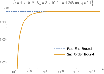
(a)

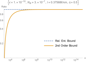
(b)

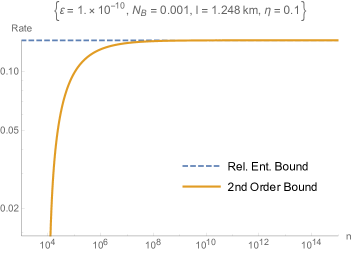
(c)

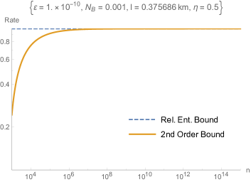
(d)

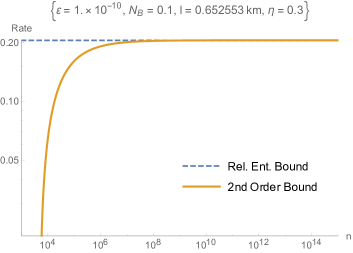
(e)

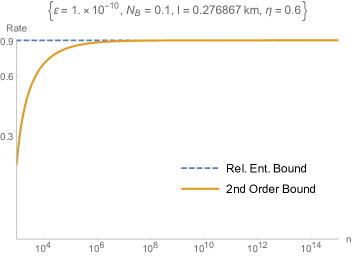
(f)

Figure 1: The figures plot upper bounds on the non-asymptotic secret-key-agreement capacity of the thermal channels of transmissivity $\eta\in(0,1)$ and thermal mean photon number $N_{B}>0$, given by the second-order approximation from (9). In each figure, we select certain values of $\eta$ (corresponding to a certain distance $L$ via $\eta=\exp[-L/L_{0}]$) and $N_{B}$, with the choices indicated above each figure. In all cases, we take the conservative value of $\varepsilon=10^{-10}$ as indicated in TCGR12 . Each figure indicates that the asymptotic secret-key-agreement capacity is too pessimistic of a benchmark for demonstrating a quantum repeater when using the channel a finite number of times. That is, there is an appreciable difference between the asymptotic and non-asymptotic secret-key-agreement capacity.

IV Results

In Figure 1, we plot upper bounds on the asymptotic secret-key-agreement capacity of the thermal channel given by (4) (dashed line) and upper bounds on the non-asymptotic secret-key-agreement capacity given by (9) (solid line) versus the number of channel uses. It is important to stress that the latter bound is only an approximation (known as the normal approximation) if $n$ is not sufficiently large (i.e., $n$ should be proportional to $1/\varepsilon^{2}$ in order for the bounds to really apply). At the same time, many prior works have shown that the normal approximation is an excellent approximation for non-asymptotic capacities even for small $n$ polyanskiy10 ; P10 ; MW12 ; P13 ; TBR15 . In each case, we choose the key-quality parameter $\varepsilon$ to be $10^{-10}$, in accordance with the same conservative value chosen in TCGR12 . In the plots, we select $\eta\in(0,1)$, (hence the corresponding distance $L$) and the thermal mean photon number $N_{B}>0$ as indicated above each figure. The distance $L$ can be related to the transmissivity $\eta$ of the thermal channel as $\eta=\exp[-L/L_{0}]$, where $L_{0}$ is the fiber attenuation length RGRKVRHWE17 . In the plots, we consider $L_{0}=0.542$ km RGRKVRHWE17 . The thermal mean photon number $N_{B}$ relevant in experimental contexts, whenever thermal noise is due exclusively to dark counts, is given by the dark counts per second times the integration period $t_{\mathrm{int}}$. In the plots, the lowest $N_{B}$ we consider corresponds to a dark count rate of $10$ per second and $t_{\mathrm{int}}=30$ ns (RGRKVRHWE17, , Section VI). For completeness, we also consider higher values of $N_{B}$, which could occur due to excessive background thermal radiation or tampering by an eavesdropper.

As noted in the introduction of our paper, these upper bounds can be interpreted to serve as benchmarks for quantum repeaters L15 . That is, the upper bounds on secret-key-agreement capacity hold for any protocol that uses the channel and LOCC but is not allowed to use a quantum repeater. As such, exceeding these upper bounds constitutes a demonstration of a quantum repeater L15 . What our results indicate is that the previous upper bounds from PLOB15 ; WTB16  on the asymptotic secret-key-agreement capacity are too pessimistic of a benchmark for protocols that are only using the channel a finite number of times. As such, the burden of demonstrating a quantum repeater is now somewhat relieved in comparison to what was previously thought would be necessary.

From an experimental perspective, it could be of interest to perform a test using the results of our paper in order to demonstrate a working quantum repeater. A convincing approach for doing so would be to conduct an actual secret-key-distillation protocol over some finite number of uses of the channel and determine what secret-key rates can be achieved. (RGRKVRHWE17, , Section IV) details methods for determining secret-key rates that are achievable in particular physical setups. For a given rate and number of channel uses, one can then compare the results with our plots (or other plots generated via the same method for different parameter values) to determine if the rate is achieved is larger than the upper bounds in our plots; if it is the case, then one can claim a working quantum repeater, albeit with the understanding that our upper bounds are the normal approximations of the true finite-length upper bounds (as discussed previously). This approach is to be contrasted with those that estimate the quantum bit-error rate from just a few channel uses and then use this parameter to calculate an asymptotic key rate (see the review in SBCDLP09 for discussions of such approaches).

V Conclusion

In this paper, we showed how to extend the teleportation simulation method of LMGA17 to the relative entropy of entanglement measure. By combining with prior results in WTB16 regarding non-asymptotic secret-key-agreement capacity, this extension leads to improved bounds on the non-asymptotic secret-key-agreement capacity of a thermal bosonic channel, in certain parameter regimes. Given that upper bounds on secret-key-agreement capacity have been advocated as a way to assess the performance of a quantum repeater, our results indicate that previous bounds from PLOB15 ; WTB16 are too pessimistic, and it should be somewhat easier to demonstrate a working quantum repeater in the realistic regime of a finite number of channel uses.

We remark that our approach can be extended to quantum amplifier channels, but we did not discuss these channels in any detail because they appear to be most prominently physically relevant in exotic relativistic communication scenarios bradler2012quantum ; bradler2015black ; QW16 . Our approach also applies to single-mode additive-noise Gaussian channels.

Going forward from here, it would be interesting to generalize our results to multimode bosonic communication channels CEGH08 or channels that are not phase-insensitive. As discussed previously TSW16 ; TSW17 ; WTB16 , it would also be good to determine bounds on performance when there is an average energy constraint at the input of each channel use. One should expect to find improved upper bounds due to this extra constraint.

Appendix A Little room for improving the strong converse bound in (1)

Here we argue why we think it will not be possible to improve upon the upper bound in (1), up to lower-order terms. Before proceeding, recall that the conditional quantum entropy and conditional entropy variance TH12 are defined for a bipartite state $\rho_{AB}$ as

$$H(A|B)_{\rho} \equiv-D(\rho_{AB}\|I_{A}\otimes\rho_{B}),$$ (48)

$$V(A|B)_{\rho} \equiv V(\rho_{AB}\|I_{A}\otimes\rho_{B}).$$ (49)

The coherent information is defined as $I(A\rangle B)_{\rho}\equiv-H(A|B)_{\rho}$ PhysRevA.54.2629  and its corresponding variance is $V(A\rangle B)_{\rho}\equiv V(A|B)_{\rho}$. In (WTB16, , Section 6.2), the following achievability bound was established for $\mathcal{N}$ a finite-dimensional channel:

$$P_{\mathcal{N}}^{\leftrightarrow}(n,\varepsilon)\geq I_{\operatorname{rev}}(\mathcal{N})+\sqrt{\frac{V_{\operatorname{rev}}^{\varepsilon}(\mathcal{N)}}{n}}\Phi^{-1}(\varepsilon)+O\!\left(\frac{\log n}{n}\right)$$ (50)

where $I_{\operatorname{rev}}(\mathcal{N})$ is the following quantity (DJKR06, , Section 5.3) (sometimes called the channel’s reverse coherent information):

$$I_{\operatorname{rev}}(\mathcal{N})\equiv\max_{|\psi\rangle_{AA^{\prime}}\in\mathcal{H}_{AA^{\prime}}}I(B\rangle A)_{\theta},$$ (51)

$\theta_{AB}\equiv\mathcal{N}_{A^{\prime}\rightarrow B}(\psi_{AA^{\prime}})$, and $V_{\operatorname{rev}}^{\varepsilon}(\mathcal{N)}$ is the channel’s reverse conditional entropy variance:

$$V_{\operatorname{rev}}^{\varepsilon}(\mathcal{N)\equiv}\left\{\begin{array}[c]{cc}\min_{\psi_{AA^{\prime}}\in\Pi_{\operatorname{rev}}}V(B\rangle A)_{\theta}&\text{for }\varepsilon<1/2\\ \max_{\psi_{AA^{\prime}}\in\Pi_{\operatorname{rev}}}V(B\rangle A)_{\theta}&\text{for }\varepsilon\geq 1/2\end{array}\right..$$ (52)

The set $\Pi_{\operatorname{rev}}\subseteq\mathcal{D}(\mathcal{H}_{AA^{\prime}})$ is the set of all states achieving the maximum in (51).

The inequality in (50) follows from a one-shot coding theorem (WTB16, , Proposition 21), followed by an expansion of the hypothesis testing relative entropy as li12 ; TH12

$$D_{H}^{\varepsilon}(\rho^{\otimes n}\|\sigma^{\otimes n})\geq\\ nD(\rho\|\sigma)+\sqrt{nV(\rho\|\sigma)}\Phi^{-1}(\varepsilon)+O(\log n).$$ (53)

A critical step employed in the above expansion is the Berry–Esseen theorem KS10 ; S11 . Rather than employing the Berry–Esseen theorem, we can modify the proof of Theorem 2 in li12  (therein instead picking $L_{n}=\exp(nD(\rho\|\sigma)-\sqrt{nV(\rho\|\sigma)/\varepsilon})$) to employ the Chebyshev inequality and instead find the following expansion:

$$D_{H}^{\varepsilon}(\rho^{\otimes n}\|\sigma^{\otimes n})\geq nD(\rho\|\sigma)-\sqrt{\frac{nV(\rho\|\sigma)}{\varepsilon}}.$$ (54)

For these theorems to hold in separable infinite-dimensional Hilbert spaces, it remains to show how to connect the coding theorem in (WTB16, , Proposition 21) to the inequality in (54), but we strongly suspect that this should be possible. If everything holds, we would obtain the following achievability theorem for an infinite-dimensional channel $\mathcal{N}$:

$$P_{\mathcal{N}}^{\leftrightarrow}(n,\varepsilon)\geq I_{\operatorname{rev}}(\mathcal{N})-\sqrt{\frac{V_{\operatorname{rev}}^{\varepsilon}(\mathcal{N)}}{n\varepsilon}}+O\!\left(\frac{1}{n}\right).$$ (55)

The above would hold for all finite-energy two-mode, squeezed vacuum states passed through the channel, and one could then take a limit as the photon number approaches infinity. The term $I_{\operatorname{rev}}(\mathcal{N})$ converges to $-\log_{2}(1-\eta)$ PLOB15 . Below we show that the relative entropy variance $V_{\operatorname{rev}}^{\varepsilon}(\mathcal{N)}$ term converges to zero. This would then give the following bound

$$P_{\mathcal{L}_{\eta}}^{\leftrightarrow}(n,\varepsilon)\geq-\log_{2}(1-\eta)+O\!\left(\frac{1}{n}\right),$$ (56)

leading us to our conclusion that there is little room for improving the upper bound in (1). We stress that this remains to be worked out in detail.

We now evaluate the variance for the reverse coherent information when sending in a two-mode squeezed vacuum to a pure-loss channel of transmissivity $\eta\in(0,1)$. Recall that the quantity of interest is

$$V(B\rangle A)$$

$$=\operatorname{Tr}\{\rho_{AB}\left[\log\rho_{AB}-\log\rho_{A}\right]^{2}\}$$ (57)

$$\qquad-\left[H(AB)_{\rho}-H(A)_{\rho}\right]^{2}$$ (58)

$$=\operatorname{Tr}\{\rho_{AB}\left[\log\rho_{AB}\right]^{2}\}$$

$$\qquad-2\operatorname{Tr}\{\rho_{AB}\log\rho_{AB}\log\rho_{A}\}+\operatorname{Tr}\{\rho_{AB}\left[\log\rho_{A}\right]^{2}\}$$

$$\qquad-\left[H(AB)_{\rho}-H(A)_{\rho}\right]^{2}$$ (59)

$$=\operatorname{Tr}\{\rho_{AB}\left[\log\rho_{AB}\right]^{2}\}-H(AB)_{\rho}^{2}$$

$$\qquad-2\left[\operatorname{Tr}\{\rho_{AB}\log\rho_{AB}\log\rho_{A}\}-H(A)_{\rho}H(AB)_{\rho}\right]$$

$$\qquad+\operatorname{Tr}\{\rho_{A}\left[\log\rho_{A}\right]^{2}\}-H(A)_{\rho}^{2}.$$ (60)

The first and last terms we can evaluate easily using the following formula for the entropy variance of a thermal state with mean photon number $N_{S}$ (WRG15, , Appendix A):

$$V(N_{S})=N_{S}\left(N_{S}+1\right)\left[\log\left(1+\frac{1}{N_{S}}\right)\right]^{2}.$$ (61)

For the first, using the notion of purification, purifying with $\psi_{ABE}$, and observing that $\psi_{E}$ is a thermal state with mean photon number $\left(1-\eta\right)N_{S}$, we find that

$$\operatorname{Tr}\{\rho_{AB}\left[\log\rho_{AB}\right]^{2}\}-H(AB)_{\rho}^{2}$$

$$=\operatorname{Tr}\{\psi_{E}\left[\log\psi_{E}\right]^{2}\}-H(E)_{\psi}^{2}$$ (62)

$$=\left(1-\eta\right)N_{S}\left(\left(1-\eta\right)N_{S}+1\right)\left[\log\left(1+\frac{1}{\left(1-\eta\right)N_{S}}\right)\right]^{2}.$$ (63)

For the last term, we observe that $\rho_{A}$ is a thermal state with mean photon number $N_{S}$, which implies that

$$\operatorname{Tr}\{\rho_{A}\left[\log\rho_{A}\right]^{2}\}-H(A)_{\rho}^{2}\\ =N_{S}\left(N_{S}+1\right)\left[\log\left(1+\frac{1}{N_{S}}\right)\right]^{2}.$$ (64)

So it remains to handle the middle term. Consider that

$$\operatorname{Tr}\{\rho_{AB}\log\rho_{AB}\log\rho_{A}\}$$

$$=\operatorname{Tr}\{\psi_{ABE}\log\rho_{AB}\log\rho_{A}\}$$ (65)

$$=\operatorname{Tr}\{\psi_{ABE}\log\psi_{E}\log\rho_{A}\}$$ (66)

$$=\operatorname{Tr}\{\psi_{AE}\log\psi_{E}\log\rho_{A}\}.$$ (67)

Consider that we can write

$$\psi_{E} =\left[\left(1-\eta\right)N_{S}+1\right]^{-1}\left(1+\frac{1}{\left(1-\eta\right)N_{S}}\right)^{-\hat{n}_{E}},$$ (68)

$$\rho_{A} =\left[N_{S}+1\right]^{-1}\left(1+\frac{1}{N_{S}}\right)^{-\hat{n}_{A}},$$ (69)

where $\hat{n}_{E}$ and $\hat{n}_{A}$ are the number operators. This means that

$$\operatorname{Tr}\{\psi_{AE}\log\psi_{E}\log\rho_{A}\}$$

$$=\operatorname{Tr}\Bigg{\{}\psi_{AE}\log\left[\left[\left(1-\eta\right)N_{S}+1\right]^{-1}\left(1+\frac{1}{\left(1-\eta\right)N_{S}}\right)^{-\hat{n}_{E}}\right]$$

$$\qquad\times\log\left[\left[N_{S}+1\right]^{-1}\left(1+\frac{1}{N_{S}}\right)^{-\hat{n}_{A}}\right]\Bigg{\}}$$ (70)

$$=\operatorname{Tr}\Bigg{\{}\psi_{AE}\log\left[\left[\left(1-\eta\right)N_{S}+1\right]\left(1+\frac{1}{\left(1-\eta\right)N_{S}}\right)^{\hat{n}_{E}}\right]$$

$$\qquad\times\log\left[\left[N_{S}+1\right]\left(1+\frac{1}{N_{S}}\right)^{\hat{n}_{A}}\right]\Bigg{\}}$$ (71)

$$=\log\left[\left(1-\eta\right)N_{S}+1\right]\log\left[N_{S}+1\right]\\ +\log\left[\left[\left(1-\eta\right)N_{S}+1\right]\right]\log\left[\left(1+\frac{1}{N_{S}}\right)\right]\operatorname{Tr}\left\{\psi_{AE}\hat{n}_{A}\right\}\\ +\log\left[1+\frac{1}{\left(1-\eta\right)N_{S}}\right]\log\left[N_{S}+1\right]\operatorname{Tr}\left\{\psi_{AE}\hat{n}_{E}\right\}\\ +\log\left[1+\frac{1}{\left(1-\eta\right)N_{S}}\right]\log\left[1+\frac{1}{N_{S}}\right]\operatorname{Tr}\left\{\psi_{AE}\left(\hat{n}_{A}\otimes\hat{n}_{E}\right)\right\}$$ (72)

$$=\log\left[\left(1-\eta\right)N_{S}+1\right]\log\left[N_{S}+1\right]\\ +N_{S}\log\left[\left[\left(1-\eta\right)N_{S}+1\right]\right]\log\left[\left(1+\frac{1}{N_{S}}\right)\right]\\ +\left(1-\eta\right)N_{S}\log\left[1+\frac{1}{\left(1-\eta\right)N_{S}}\right]\log\left[N_{S}+1\right]\\ +\log\left[1+\frac{1}{\left(1-\eta\right)N_{S}}\right]\log\left[1+\frac{1}{N_{S}}\right]\times\\ \operatorname{Tr}\left\{\psi_{AE}\left(\hat{n}_{A}\otimes\hat{n}_{E}\right)\right\}.$$ (73)

We note that the third equality follows by applying the identity $\log(ab^{\hat{x}})=\log(a)+\hat{x}\log(b)$ for positive scalars $a$ and $b$ and a positive operator $\hat{x}$. So we need to evaluate the term $\operatorname{Tr}\left\{\psi_{AE}\left(\hat{n}_{A}\otimes\hat{n}_{E}\right)\right\}$. Consider that sending a number state $|n\rangle\langle n|$ through a beamsplitter of transmissivity $1-\eta$ leads to the following transformation:

$$|n\rangle\langle n|_{A^{\prime}}\rightarrow\sum_{k=0}^{n}\binom{n}{k}\left(1-\eta\right)^{k}\eta^{n-k}|k\rangle\langle k|_{E}.$$ (74)

The two-mode squeezed vacuum at the input has the following form:

$$\frac{1}{\sqrt{N_{S}+1}}\sum_{n=0}^{\infty}\sqrt{\left(\frac{N_{S}}{N_{S}+1}\right)^{n}}|n\rangle_{A}|n\rangle_{A^{\prime}}.$$ (75)

However since we are evaluating $\operatorname{Tr}\left\{\psi_{AE}\left(\hat{n}_{A}\otimes\hat{n}_{E}\right)\right\}$, and $\hat{n}_{A}$ and $\hat{n}_{E}$ are diagonal in the number basis, this is equivalent to the following:

$$\frac{1}{N_{S}+1}\sum_{n=0}^{\infty}\sum_{k=0}^{n}\left(\frac{N_{S}}{N_{S}+1}\right)^{n}\binom{n}{k}\left(1-\eta\right)^{k}\eta^{n-k}\times$$

$$\qquad\operatorname{Tr}\{\left(|n\rangle\langle n|_{A}\otimes|k\rangle\langle k|\right)\left(\hat{n}_{A}\otimes\hat{n}_{E}\right)\}$$

$$=\frac{1}{N_{S}+1}\sum_{n=0}^{\infty}\sum_{k=0}^{n}\left(\frac{N_{S}}{N_{S}+1}\right)^{n}\binom{n}{k}\left(1-\eta\right)^{k}\eta^{n-k}nk$$ (76)

$$=\frac{1}{N_{S}+1}\sum_{n=0}^{\infty}n\left(\frac{N_{S}}{N_{S}+1}\right)^{n}\sum_{k=0}^{n}\binom{n}{k}\left(1-\eta\right)^{k}\eta^{n-k}k.$$ (77)

Consider that the expression $\sum_{k=0}^{n}\binom{n}{k}\left(1-\eta\right)^{k}\eta^{n-k}k$ is equal to the mean of a binomial random variable with parameter $1-\eta$, and so

$$\sum_{k=0}^{n}\binom{n}{k}\left(1-\eta\right)^{k}\eta^{n-k}k=n\left(1-\eta\right),$$ (78)

implying that the last line above is equal to

$$\left(1-\eta\right)\frac{1}{N_{S}+1}\sum_{n=0}^{\infty}n^{2}\left(\frac{N_{S}}{N_{S}+1}\right)^{n}.$$ (79)

This is then equal to the second moment of a geometric random variable with parameter $p=1/\left(N_{S}+1\right)$, so that

$$\left(1-\eta\right)\frac{1}{N_{S}+1}\sum_{n=0}^{\infty}n^{2}\left(\frac{N_{S}}{N_{S}+1}\right)^{n}$$

$$=\left(1-\eta\right)\left(N_{S}\left(N_{S}+1\right)+N_{S}^{2}\right)$$ (80)

$$=\left(1-\eta\right)N_{S}\left(2N_{S}+1\right).$$ (81)

Plugging into the above, we find the reduction

$$=\log\left[\left(1-\eta\right)N_{S}+1\right]\log\left[N_{S}+1\right]\\ +N_{S}\log\left[\left[\left(1-\eta\right)N_{S}+1\right]\right]\log\left[\left(1+\frac{1}{N_{S}}\right)\right]\\ +\left(1-\eta\right)N_{S}\log\left[1+\frac{1}{\left(1-\eta\right)N_{S}}\right]\log\left[N_{S}+1\right]\\ +\left(1-\eta\right)N_{S}\left(2N_{S}+1\right)\log\left[1+\frac{1}{\left(1-\eta\right)N_{S}}\right]\log\left[1+\frac{1}{N_{S}}\right].$$ (82)

From this we should subtract the following quantity

$$H(A)_{\rho}H(AB)_{\rho}$$

$$=g(N_{S})g(\left(1-\eta\right)N_{S})$$ (83)

$$=\left[\left(N_{S}+1\right)\log\left(N_{S}+1\right)-N_{S}\log N_{S}\right]\times$$

$$\left[\begin{array}[c]{c}\left(\left(1-\eta\right)N_{S}+1\right)\log\left(\left(1-\eta\right)N_{S}+1\right)\\ -\left(1-\eta\right)N_{S}\log\left(1-\eta\right)N_{S}\end{array}\right]$$ (86)

$$=\left[N_{S}\log\left(1+\frac{1}{N_{S}}\right)+\log\left(N_{S}+1\right)\right]\times$$

$$\left[\left(1-\eta\right)N_{S}\log\left(1+\frac{1}{\left(1-\eta\right)N_{S}}\right)+\log\left(\left(1-\eta\right)N_{S}+1\right)\right]$$ (87)

$$=\left(1-\eta\right)N_{S}^{2}\log\left(1+\frac{1}{N_{S}}\right)\log\left(1+\frac{1}{\left(1-\eta\right)N_{S}}\right)\\ +\left(1-\eta\right)N_{S}\log\left(N_{S}+1\right)\log\left(1+\frac{1}{\left(1-\eta\right)N_{S}}\right)\\ +N_{S}\log\left(1+\frac{1}{N_{S}}\right)\log\left(\left(1-\eta\right)N_{S}+1\right)\\ +\log\left(N_{S}+1\right)\log\left(\left(1-\eta\right)N_{S}+1\right),$$ (88)

leading to

$$\operatorname{Tr}\{\rho_{AB}\log\rho_{AB}\log\rho_{A}\}-H(A)_{\rho}H(AB)_{\rho}$$

$$=\left(1-\eta\right)N_{S}\left(2N_{S}+1\right)\log\left[1+\frac{1}{\left(1-\eta\right)N_{S}}\right]\log\left[1+\frac{1}{N_{S}}\right]$$

$$\qquad-\left(1-\eta\right)N_{S}^{2}\log\left(1+\frac{1}{N_{S}}\right)\log\left(1+\frac{1}{\left(1-\eta\right)N_{S}}\right)$$ (89)

$$=\left(1-\eta\right)N_{S}\left(N_{S}+1\right)\log\left[1+\frac{1}{\left(1-\eta\right)N_{S}}\right]\log\left[1+\frac{1}{N_{S}}\right].$$ (90)

Putting everything together, we find that the variance of the reverse coherent information is given by

$$\left(1-\eta\right)N_{S}\left(\left(1-\eta\right)N_{S}+1\right)\left[\log\left(1+\frac{1}{\left(1-\eta\right)N_{S}}\right)\right]^{2}\\ -2\left(1-\eta\right)N_{S}\left(N_{S}+1\right)\log\left[1+\frac{1}{\left(1-\eta\right)N_{S}}\right]\log\left[1+\frac{1}{N_{S}}\right]\\ +N_{S}\left(N_{S}+1\right)\left[\log\left(1+\frac{1}{N_{S}}\right)\right]^{2}.$$ (91)

For large $N_{S}$, we have that $\left(\left(1-\eta\right)N_{S}+1\right)\approx\left(1-\eta\right)N_{S}$ and $\left(N_{S}+1\right)\approx N_{S}$, so that the above reduces to

$$\approx\left[\left(1-\eta\right)N_{S}\log\left(1+\frac{1}{\left(1-\eta\right)N_{S}}\right)-N_{S}\log\left(1+\frac{1}{N_{S}}\right)\right]^{2},$$ (92)

which converges to zero as $N_{S}\rightarrow\infty$.

Appendix B Weak converse bounds for secret-key-agreement capacities

Here we argue for the weak-converse bounds given in (2) and (8), and even more general weak-converse bounds. The weak-converse bounds are a direct consequence of the bounds in WTB16 and (WR12, , Eq. (2)) (see also (MW12, , Eq. (134))).

First, recall from (WR12, , Eq. (2)) and (MW12, , Eq. (134)) that the following bound holds for hypothesis testing relative entropy for $\varepsilon\in(0,1)$:

$$D_{H}^{\varepsilon}(\rho\|\sigma)\leq\frac{1}{1-\varepsilon}\left[D(\rho\|\sigma)+h_{2}(\varepsilon)\right].$$ (93)

To see this, consider that the definition of $D_{H}^{\varepsilon}(\rho\|\sigma)$ can be further constrained as

$$D_{H}^{\varepsilon}(\rho\|\sigma)=\\ -\log_{2}\inf_{\Lambda}\{\operatorname{Tr}\{\Lambda\sigma\}:0\leq\Lambda\leq I\wedge\operatorname{Tr}\{\Lambda\rho\}=1-\varepsilon\}.$$ (94)

That is, it suffices to optimize over measurement operators that meet the constraint $\operatorname{Tr}\{\Lambda\rho\}\geq 1-\varepsilon$ with equality. This follows because for any measurement operator $\Lambda$ such that $\operatorname{Tr}\{\Lambda\rho\}>1-\varepsilon$, we can modify it by scaling it by a positive number $\lambda\in(0,1)$ such that $\operatorname{Tr}\{\left(\lambda\Lambda\right)\rho\}=1-\varepsilon$. The new operator $\lambda\Lambda$ is a legitimate measurement operator and the error probability $\operatorname{Tr}\{(\lambda\Lambda)\sigma\}$ only decreases under this scaling (i.e., $\operatorname{Tr}\{(\lambda\Lambda)\sigma\}<\operatorname{Tr}\{\Lambda\sigma\}$), which allows us to conclude (94). Now for any measurement operator $\Lambda$ such that $\operatorname{Tr}\{\Lambda\rho\}=1-\varepsilon$, the monotonicity of quantum relative entropy Lindblad1975 with respect to quantum channels implies that

$$D(\rho\|\sigma)$$

$$\geq D(\{1-\varepsilon,\varepsilon\}\|\{\operatorname{Tr}\{\Lambda\sigma\},1-\operatorname{Tr}\{\Lambda\sigma\}\})$$ (95)

$$=(1-\varepsilon)\log_{2}\left(\frac{1-\varepsilon}{\operatorname{Tr}\{\Lambda\sigma\}}\right)+\varepsilon\log_{2}\!\left(\frac{\varepsilon}{1-\operatorname{Tr}\{\Lambda\sigma\}}\right)$$ (96)

$$=-\left(1-\varepsilon\right)\log_{2}\operatorname{Tr}\{\Lambda\sigma\}-h_{2}(\varepsilon)$$

$$\qquad\qquad+\varepsilon\log_{2}\!\left(\frac{1}{1-\operatorname{Tr}\{\Lambda\sigma\}}\right)$$ (97)

$$\geq-\left(1-\varepsilon\right)\log_{2}\operatorname{Tr}\{\Lambda\sigma\}-h_{2}(\varepsilon).$$ (98)

Rewriting this gives

$$-\log\operatorname{Tr}\{\Lambda\sigma\}\leq\frac{1}{1-\varepsilon}\left[D(\rho\|\sigma)+h_{2}(\varepsilon)\right].$$ (99)

Since this bound holds for all measurement operators $\Lambda$ satisfying $\operatorname{Tr}\{\Lambda\rho\}=1-\varepsilon$, we can conclude (93).

To conclude the desired weak-converse bounds, we then invoke the above and (WTB16, , Eq. (4.34)) to get that the following bound holds for any teleportation simulable channel with associated resource state $\omega_{AB}$:

$$P_{\mathcal{N}}^{\leftrightarrow}(n,\varepsilon) \leq\frac{1}{n}E_{R}^{\varepsilon}(A^{n};B^{n})_{\omega^{\otimes n}}$$ (100)

$$\leq\frac{1}{n(1-\varepsilon)}\left[E_{R}(A^{n};B^{n})_{\omega^{\otimes n}}+h_{2}(\varepsilon)\right]$$ (101)

$$\leq\frac{1}{(1-\varepsilon)}\left[E_{R}(A;B)_{\omega}+\frac{h_{2}(\varepsilon)}{n}\right].$$ (102)

If the channel requires an infinite-energy resource state to become teleportation simulable, then one must take care as in the case of the proofs in (WTB16, , Section 8), and then one finally arrives at the weak-converse bounds in (2) and (8).

Appendix C Asymptotic equipartition property for hypothesis testing relative entropy

In this appendix, we prove that the inequality in (38) holds whenever the states $\rho$ and $\sigma$ involved act on a separable Hilbert space. Here we take the convention, for convenience, that all logarithms are with respect to the natural base, but we note that the bound (105) applies equally well for the binary logarithm just by rescaling.

The following proposition is available as (JOPS12, , Eq. (6.5)) and restated as (DPR15, , Corollary 2):

Proposition 1 ((JOPS12, , Eq. (6.5)))

Let $\rho$ and $\sigma$ be faithful states acting on a separable Hilbert space $\mathcal{H}$, let $\Lambda$ be a measurement operator acting on $\mathcal{H}$ and such that $0\leq\Lambda\leq I$, and let $v,\theta\in\mathbb{R}$. Then

$$e^{-\theta}\operatorname{Tr}\{(I-\Lambda)\rho\}+\operatorname{Tr}\{\Lambda\sigma\}\geq\frac{e^{-\theta}}{1+e^{v-\theta}}\Pr\{X\leq v\},$$ (103)

where $X$ is a random variable taking values $\log(\lambda_{x}/\mu_{y})$ with probability $\left|\left\langle\psi_{y}|\phi_{x}\right\rangle\right|^{2}\lambda_{x}$, where these quantities are defined in (31) and (32).

The following proposition is based on ideas given in DPR15 :

Proposition 2

Let $\rho$ and $\sigma$ be faithful states acting on a separable Hilbert space $\mathcal{H}$, such that

$$D(\rho\|\sigma),\ V(\rho\|\sigma),\ T(\rho\|\sigma) <\infty,$$

$$V(\rho\|\sigma) >0.$$ (104)

Then the following bound holds for all $\varepsilon\in(0,1)$ and sufficiently large $n$:

$$D_{H}^{\varepsilon}(\rho^{\otimes n}\|\sigma^{\otimes n})\leq\\ nD(\rho\|\sigma)+\sqrt{nV(\rho\|\sigma)}\Phi^{-1}(\varepsilon)+O(\log n).$$ (105)

Proof. We follow the justification for Theorem 3 given in DPR15 closely, but we do make some slight changes after the first few steps. Let $\Lambda^{n}$ be any measurement operator satisfying $\operatorname{Tr}\{\left(I^{\otimes n}-\Lambda^{n}\right)\rho^{\otimes n}\}\leq\varepsilon$. By applying the above proposition (making the replacements $\rho\rightarrow\rho^{\otimes n}$ and $\sigma\rightarrow\sigma^{\otimes n}$, so that $X_{n}$ is a sum of $n$ i.i.d. random variables, each having mean $D(\rho\|\sigma)$, variance $V(\rho\|\sigma)$, and third absolute central moment $T(\rho\|\sigma)$), we find that

$$\operatorname{Tr}\{\Lambda^{n}\sigma^{\otimes n}\}$$

$$\geq e^{-\theta_{n}}\left(\frac{\Pr\{X_{n}\leq v_{n}\}}{1+e^{v_{n}-\theta_{n}}}-\operatorname{Tr}\{(I-\Lambda^{n})\rho^{\otimes n}\}\right)$$ (106)

$$\geq e^{-\theta_{n}}\left(\frac{\Pr\{X_{n}\leq v_{n}\}}{1+e^{v_{n}-\theta_{n}}}-\varepsilon\right).$$ (107)

The Berry–Esseen theorem KS10 ; S11 implies for any real number $a$ that

$$\Pr\left\{\frac{X_{n}-nD(\rho\|\sigma)}{\sqrt{nV(\rho\|\sigma)}}\leq a\right\}\geq\Phi(a)-K_{\rho,\sigma}\,n^{-1/2},$$ (108)

where

$$K_{\rho,\sigma}\equiv\frac{C\,T(\rho\|\sigma)}{[V(\rho\|\sigma)]^{3/2}}$$ (109)

and $C\in(0,0.4748)$ KS10 ; S11 . It is clear that $K_{\rho,\sigma}$ is a strictly positive constant $>C$ due to the assumption in (104) and the fact that $T(\rho\|\sigma)\geq[V(\rho\|\sigma)]^{3/2}$ S11 . Let us set

$$v_{n}=nD(\rho\|\sigma)+\\ \sqrt{nV(\rho\|\sigma)}\Phi^{-1}(\varepsilon+(2+K_{\rho,\sigma})n^{-1/2}),$$ (110)

and note that we require sufficiently large $n$ here, so that the argument to $\Phi^{-1}$ is $\in(0,1)$. We then find that

$$\operatorname{Tr}\{\Lambda^{n}\sigma^{\otimes n}\}\geq e^{-\theta_{n}}\left(\frac{\varepsilon+2n^{-1/2}}{1+e^{v_{n}-\theta_{n}}}-\varepsilon\right).$$ (111)

Now choosing $\theta_{n}=v_{n}+\frac{1}{2}\log n$, we get that

$$\operatorname{Tr}\{\Lambda^{n}\sigma^{\otimes n}\}\geq\\ \left[e^{-nD(\rho\|\sigma)-\sqrt{nV(\rho\|\sigma)}\Phi^{-1}(\varepsilon+(2+K_{\rho,\sigma})n^{-1/2})-\frac{1}{2}\log n}\right]\times\\ \left(\frac{1}{1+n^{-1/2}}\right),$$ (112)

so that the following inequality holds for sufficiently large $n$:

$$-\log\operatorname{Tr}\{\Lambda^{n}\sigma^{\otimes n}\}\leq\\ nD(\rho\|\sigma)+\sqrt{nV(\rho\|\sigma)}\Phi^{-1}(\varepsilon)+O(\log n).$$ (113)

In the last line, we have invoked (TH12, , Footnote 6), which in turn is an invocation of Taylor’s theorem: for $f$ continuously differentiable, $c$ a positive constant, and $n\geq n_{0}$, the following equality holds

$$\sqrt{n}f(x+c/\sqrt{n})=\sqrt{n}f(x)+cf^{\prime}(a)$$ (114)

for some $a\in[x,x+c/\sqrt{n_{0}}]$.   

Appendix D Finiteness of the third absolute central moment of the log likelihood ratio for quantum Gaussian states

We argue in this final appendix that $T(\rho\|\sigma)$, the third absolute central moment of the log-likelihood ratio of two finite-energy, zero-mean Gaussian states $\rho$ and $\sigma$, is finite. By definition, we have that

$$T(\rho\|\sigma)=\sum_{x,y}\left|\left\langle\psi_{y}|\phi_{x}\right\rangle\right|^{2}\lambda_{x}\left|\log_{2}\left(\lambda_{x}/\mu_{y}\right)-D(\rho\|\sigma)\right|^{3},$$ (115)

where the spectral decompositions of $\rho$ and $\sigma$ are given by

$$\rho=\sum_{x}\lambda_{x}|\phi_{x}\rangle\langle\phi_{x}|,\qquad\sigma=\sum_{y}\mu_{y}|\psi_{y}\rangle\langle\psi_{y}|.$$ (116)

By concavity of $x^{3/4}$ for $x\geq 0$, it follows that

$$T(\rho\|\sigma)\\ =\sum_{x,y}\left|\left\langle\psi_{y}|\phi_{x}\right\rangle\right|^{2}\lambda_{x}\left[\left|\log_{2}\left(\lambda_{x}/\mu_{y}\right)-D(\rho\|\sigma)\right|^{4}\right]^{3/4}\\ \leq\left[\sum_{x,y}\left|\left\langle\psi_{y}|\phi_{x}\right\rangle\right|^{2}\lambda_{x}\left|\log_{2}\left(\lambda_{x}/\mu_{y}\right)-D(\rho\|\sigma)\right|^{4}\right]^{3/4}\\ =\left[\sum_{x,y}\left|\left\langle\psi_{y}|\phi_{x}\right\rangle\right|^{2}\lambda_{x}\left(\log_{2}\left(\lambda_{x}/\mu_{y}\right)-D(\rho\|\sigma)\right)^{4}\right]^{3/4},$$ (117)

and so we aim to show that this latter quantity is finite. For zero-mean, $m$-mode faithful Gaussian states, the Williamson theorem W36 implies that their spectral decompositions are as follows:

$$\rho =U_{\rho}\left(\bigotimes\limits_{i=1}^{m}\theta(N_{\rho}^{i})\right)U_{\rho}^{{\dagger}},$$ (118)

$$\sigma =U_{\sigma}\left(\bigotimes\limits_{i=1}^{m}\theta(N_{\sigma}^{i})\right)U_{\sigma}^{{\dagger}},$$ (119)

where $U_{\rho}$ and $U_{\sigma}$ denote Gaussian unitaries that can be generated by a Hamiltonian no more than quadratic in the position- and momentum-quadrature operators, $N_{\rho}^{i},N_{\sigma}^{i}>0$ for all $i$, and $\theta(N)$ denotes a thermal state of mean photon number $N$:

$$\theta(N)=\frac{1}{N+1}\sum_{n=0}^{\infty}\left(\frac{N}{N+1}\right)^{n}|n\rangle\langle n|,$$ (120)

with $|n\rangle$ denoting a photonic number state. Introducing the multi-index notation $|\vec{n}\rangle=|n_{1}\rangle\cdots|n_{m}\rangle$, we can then write the overlap $\left|\left\langle\psi_{y}|\phi_{x}\right\rangle\right|^{2}$ as $\left|\langle\vec{l}|U_{\sigma}^{{\dagger}}U_{\rho}|\vec{n}\rangle\right|^{2}$. This conditional probability distribution represents the probability of detecting the photon numbers $\vec{l}$ if the photon number state $|\vec{n}\rangle$ is prepared and transmitted through the Gaussian unitary $U_{\sigma}^{{\dagger}}U_{\rho}\equiv V$. This distribution has well defined (finite) higher moments with respect to photon number. Setting $\hat{n}_{i}$ to be the photon number operator for the $i$th mode, this claim follows because the $k$th moment of the conditional probability distribution $\left|\langle\vec{l}|U_{\sigma}^{{\dagger}}U_{\rho}|\vec{n}\rangle\right|^{2}$ is given by

$$\operatorname{Tr}\left\{V|\vec{n}\rangle\langle\vec{n}|V^{{\dagger}}\left(\sum_{i=1}^{m}\hat{n}_{i}\right)^{k}\right\}\\ =\operatorname{Tr}\left\{|\vec{n}\rangle\langle\vec{n}|\left(\sum_{i=1}^{m}V^{{\dagger}}\hat{n}_{i}V\right)^{k}\right\}.$$ (121)

Since $V$ is a Gaussian unitary generated by a Hamiltonian no more than quadratic in the position and momentum-quadrature operators S17 , each $V^{{\dagger}}\hat{n}_{i}V$ is a bounded linear combination of position and momentum-quadrature operators and so $\left(\sum_{i=1}^{m}V^{{\dagger}}\hat{n}_{i}V\right)^{k}$ is as well since $k$ is finite. Given that the photon number states have bounded moments, we can conclude that (121) is finite. The eigenvalues $\lambda_{x}$ and $\mu_{y}$ in this case are given by

$$\prod\limits_{i=1}^{m}\left[\frac{1}{N_{\rho}^{i}+1}\left(\frac{N_{\rho}^{i}}{N_{\rho}^{i}+1}\right)^{n_{i}}\right],$$ (122)

$$\prod\limits_{i=1}^{m}\left[\frac{1}{N_{\sigma}^{i}+1}\left(\frac{N_{\sigma}^{i}}{N_{\sigma}^{i}+1}\right)^{l_{i}}\right],$$ (123)

and indexed by the multi-indices $\vec{n}$ and $\vec{l}$, respectively. The distribution in (122) has well defined (finite) higher moments with respect to photon number because it is a product of geometric distributions. We can then write $\log_{2}\!\left(\lambda_{x}/\mu_{y}\right)=\log_{2}\!\left(\lambda_{x}\right)-\log_{2}\!\left(\mu_{y}\right)$ as

$$\sum_{i=1}^{m}\log_{2}\!\left(\frac{N_{\sigma}^{i}+1}{N_{\rho}^{i}+1}\right)+n_{i}\log_{2}\!\left(\frac{N_{\rho}^{i}}{N_{\rho}^{i}+1}\right)\\ -l_{i}\log_{2}\!\left(\frac{N_{\sigma}^{i}}{N_{\sigma}^{i}+1}\right).$$ (124)

Thus, after expanding, the last quantity in brackets in (117) is equal to an expression involving no more than the fourth moments of photon numbers, but we have already argued that this is finite for the distributions under question. As a consequence, we can conclude that $T(\rho\|\sigma)$ is finite whenever $\rho$ and $\sigma$ are zero-mean, finite-energy, faithful Gaussian states.

References

- [1] Alexander S. Holevo. Quantum systems, channels, information: a mathematical introduction, volume 16. Walter de Gruyter, 2012.
- [2] Masahito Hayashi. Quantum Information: An Introduction. Springer, 2006.
- [3] Mark M. Wilde. From Classical to Quantum Shannon Theory. March 2016. arXiv:1106.1445v7.
- [4] Charles H. Bennett and Gilles Brassard. Quantum cryptography: Public key distribution and coin tossing. In Proceedings of IEEE International Conference on Computers Systems and Signal Processing, pages 175–179, Bangalore, India, December 1984.
- [5] Artur K. Ekert. Quantum cryptography based on Bell’s theorem. Physical Review Letters, 67(6):661–663, August 1991.
- [6] Masahiro Takeoka, Saikat Guha, and Mark M. Wilde. The squashed entanglement of a quantum channel. IEEE Transactions on Information Theory, 60(8):4987–4998, August 2014. arXiv:1310.0129.
- [7] Masahiro Takeoka, Saikat Guha, and Mark M. Wilde. Fundamental rate-loss tradeoff for optical quantum key distribution. Nature Communications, 5:5235, October 2014. arXiv:1504.06390.
- [8] Kaushik P. Seshadreesan, Masahiro Takeoka, and Mark M. Wilde. Bounds on entanglement distillation and secret key agreement for quantum broadcast channels. IEEE Transactions on Information Theory, 62(5):2849–2866, May 2016. arXiv:1503.08139.
- [9] Stefano Pirandola, Riccardo Laurenza, Carlo Ottaviani, and Leonardo Banchi. Fundamental limits of repeaterless quantum communications. April 2016. arXiv:1510.08863v5.
- [10] Kenneth Goodenough, David Elkouss, and Stephanie Wehner. Assessing the performance of quantum repeaters for all phase-insensitive Gaussian bosonic channels. New Journal of Physics, 18(6):063005, June 2016. arXiv:1511.08710.
- [11] Masahiro Takeoka, Kaushik P. Seshadreesan, and Mark M. Wilde. Unconstrained distillation capacities of a pure-loss bosonic broadcast channel. In 2016 IEEE International Symposium on Information Theory (ISIT), pages 2484–2488, July 2016.
- [12] Koji Azuma, Akihiro Mizutani, and Hoi-Kwong Lo. Fundamental rate-loss trade-off for the quantum internet. Nature Communications, 7:13523, November 2016. arXiv:1601.02933.
- [13] Mark M. Wilde, Marco Tomamichel, and Mario Berta. Converse bounds for private communication over quantum channels. IEEE Transactions on Information Theory, 63(3):1792–1817, March 2017. arXiv:1602.08898.
- [14] Matthias Christandl and Alexander Müller-Hermes. Relative entropy bounds on quantum, private and repeater capacities. Communications in Mathematical Physics, 353(2):821–852, July 2017. arXiv:1604.03448.
- [15] Mark M. Wilde. Squashed entanglement and approximate private states. Quantum Information Processing, 15(11):4563–4580, November 2016. arXiv:1606.08028.
- [16] Stefan Bäuml and Koji Azuma. Fundamental limitation on quantum broadcast networks. Quantum Science and Technology, 2(2):024004, June 2017. arXiv:1609.03994.
- [17] Filip Rozpedek, Kenneth Goodenough, Jeremy Ribeiro, Norbert Kalb, Valentina Caprara Vivoli, Andreas Reiserer, Ronald Hanson, Stephanie Wehner, and David Elkouss. Realistic parameter regimes for a single sequential quantum repeater. May 2017. arXiv:1705.00043.
- [18] Masahiro Takeoka, Kaushik P. Seshadreesan, and Mark M. Wilde. Unconstrained capacities of quantum key distribution and entanglement distillation for pure-loss bosonic broadcast channels. June 2017. arXiv:1706.06746.
- [19] Norbert Lütkenhaus and Saikat Guha. Quantum repeaters: Objectives, definitions and architectures. Available at http://wqrn.pratt.duke.edu/presentations.html, May 2015.
- [20] Ligong Wang and Renato Renner. One-shot classical-quantum capacity and hypothesis testing. Physical Review Letters, 108(20):200501, May 2012. arXiv:1007.5456.
- [21] William Matthews and Stephanie Wehner. Finite blocklength converse bounds for quantum channels. IEEE Transactions on Information Theory, 60(11):7317–7329, November 2014. arXiv:1210.4722.
- [22] Horace Yuen and Jeffrey H. Shapiro. Optical communication with two-photon coherent states–Part I: Quantum-state propagation and quantum-noise. IEEE Transactions on Information Theory, 24(6):657–668, November 1978.
- [23] Jeffrey H. Shapiro. The quantum theory of optical communications. IEEE Journal of Selected Topics in Quantum Electronics, 15(6):1547–1569, November 2009.
- [24] Ryo Namiki and Takuya Hirano. Practical limitation for continuous-variable quantum cryptography using coherent states. Physical Review Letters, 92(11):117901, March 2004. arXiv:quant-ph/0403115.
- [25] Jérôme Lodewyck, Thierry Debuisschert, Rosa Tualle-Brouri, and Philippe Grangier. Controlling excess noise in fiber-optics continuous-variable quantum key distribution. Physical Review A, 72(5):050303, November 2005. arXiv:quant-ph/0511104.
- [26] V. Yu. Korolev and Irina G. Shevtsova. On the upper bound for the absolute constant in the Berry-Esseen inequality. Theory of Probability & Its Applications, 54(4):638–658, November 2010.
- [27] Irina Shevtsova. On the absolute constants in the Berry-Esseen type inequalities for identically distributed summands. November 2011. arXiv:1111.6554.
- [28] Yury Polyanskiy, H. Vincent Poor, and Sergio Verdú. Channel coding rate in the finite blocklength regime. IEEE Transactions on Information Theory, 56(5):2307–2359, May 2010.
- [29] Yury Polyanskiy. Channel coding: non-asymptotic fundamental limits. PhD thesis, Princeton University, November 2010.
- [30] Yury Polyanskiy. Finite blocklength methods in channel coding. Tutorial at the 2013 International Symposium on Information Theory, 2013. Available at http://people.lids.mit.edu/yp/homepage/data/ISIT13_tutorial.pdf.
- [31] Marco Tomamichel, Mario Berta, and Joseph M. Renes. Quantum coding with finite resources. Nature Communications, 7:11419, May 2016. arXiv:1504.04617.
- [32] Pietro Liuzzo-Scorpo, Andrea Mari, Vittorio Giovannetti, and Gerardo Adesso. Optimal continuous variable quantum teleportation with limited resources. Physical Review Letters, 119(12):120503, September 2017. arXiv:1705.03017.
- [33] Gerardo Adesso, Sammy Ragy, and Antony R. Lee. Continuous variable quantum information: Gaussian states and beyond. Open Systems and Information Dynamics, 21(01–02):1440001, June 2014. arXiv:1401.4679.
- [34] Alessio Serafini. Quantum Continuous Variables. CRC Press, 2017.
- [35] Charles H. Bennett, David P. DiVincenzo, John A. Smolin, and William K. Wootters. Mixed-state entanglement and quantum error correction. Physical Review A, 54(5):3824–3851, November 1996. arXiv:quant-ph/9604024.
- [36] Michael M. Wolf, David Pérez-García, and Geza Giedke. Quantum capacities of bosonic channels. Physical Review Letters, 98(13):130501, March 2007. arXiv:quant-ph/0606132.
- [37] Julien Niset, Jaromír Fiurasek, and Nicolas J. Cerf. No-go theorem for Gaussian quantum error correction. Physical Review Letters, 102(12):120501, March 2009. arXiv:0811.3128.
- [38] Alexander Müller-Hermes. Transposition in quantum information theory. Master’s thesis, Technical University of Munich, September 2012.
- [39] John Williamson. On the algebraic problem concerning the normal forms of linear dynamical systems. American Journal of Mathematics, 58(1):141–163, January 1936.
- [40] Xiao-yu Chen. Gaussian relative entropy of entanglement. Physical Review A, 71(6):062320, June 2005. arXiv:quant-ph/0402109.
- [41] Ole Krueger. Quantum Information Theory with Gaussian Systems. PhD thesis, Technische Universität Braunschweig, April 2006. Available at https://publikationsserver.tu-braunschweig.de/receive/dbbs_mods_00020741.
- [42] Alexander S. Holevo. The entropy gain of infinite-dimensional quantum channels. Doklady Mathematics, 82(2):730–731, October 2010. arXiv:1003.5765.
- [43] Lu-Ming Duan, G. Giedke, J. I. Cirac, and P. Zoller. Inseparability criterion for continuous variable systems. Physical Review Letters, 84(12):2722–2725, March 2000. arXiv:quant-ph/9908056.
- [44] R. Simon. Peres-Horodecki separability criterion for continuous variable systems. Physical Review Letters, 84(12):2726–2729, March 2000. arXiv:quant-ph/9909044.
- [45] Alessio Serafini, Fabrizio Illuminati, and Silvio De Siena. Symplectic invariants, entropic measures and correlations of gaussian states. Journal of Physics B: Atomic, Molecular and Optical Physics, 37(2):L21, January 2004. arXiv:quant-ph/0307073.
- [46] Gerardo Adesso and Fabrizio Illuminati. Gaussian measures of entanglement versus negativities: Ordering of two-mode Gaussian states. Physical Review A, 72(3):032334, September 2005. arXiv:quant-ph/0506124.
- [47] Filippo Caruso, Jens Eisert, Vittorio Giovannetti, and Alexander S. Holevo. Multi-mode bosonic Gaussian channels. New Journal of Physics, 10:083030, August 2008. arXiv:0804.0511.
- [48] Charles H. Bennett, Gilles Brassard, Claude Crépeau, Richard Jozsa, Asher Peres, and William K. Wootters. Teleporting an unknown quantum state via dual classical and Einstein-Podolsky-Rosen channels. Physical Review Letters, 70(13):1895–1899, March 1993.
- [49] Samuel L. Braunstein and H. J. Kimble. Teleportation of continuous quantum variables. Physical Review Letters, 80(4):869–872, January 1998.
- [50] Reinhard F. Werner. All teleportation and dense coding schemes. Journal of Physics A: Mathematical and General, 34(35):7081, September 2001. arXiv:quant-ph/0003070.
- [51] Mark M. Wilde, Marco Tomamichel, and Mario Berta. Converse bounds for private communication over quantum channels. January 2016. 1602.08898v1.
- [52] Ryo Namiki. Teleportation stretching for lossy Gaussian channels. March 2016. arXiv:1603.05292.
- [53] Ryszard Horodecki, Pawel Horodecki, Michal Horodecki, and Karol Horodecki. Quantum entanglement. Reviews of Modern Physics, 81(2):865–942, June 2009. arXiv:quant-ph/0702225.
- [54] Hisaharu Umegaki. Conditional expectations in an operator algebra IV (entropy and information). Kodai Mathematical Seminar Reports, 14(2):59–85, 1962.
- [55] Göran Lindblad. Entropy, information and quantum measurements. Communications in Mathematical Physics, 33(4):305–322, December 1973.
- [56] Ke Li. Second order asymptotics for quantum hypothesis testing. Annals of Statistics, 42(1):171–189, February 2014. arXiv:1208.1400.
- [57] Marco Tomamichel and Masahito Hayashi. A hierarchy of information quantities for finite block length analysis of quantum tasks. IEEE Transactions on Information Theory, 59(11):7693–7710, November 2013. arXiv:1208.1478.
- [58] Francesco Buscemi and Nilanjana Datta. The quantum capacity of channels with arbitrarily correlated noise. IEEE Transactions on Information Theory, 56(3):1447–1460, March 2010. arXiv:0902.0158.
- [59] Mark M. Wilde, Marco Tomamichel, Seth Lloyd, and Mario Berta. Gaussian hypothesis testing and quantum illumination. Physical Review Letters, 119(12):120501, September 2017. arXiv:1608.06991.
- [60] Nilanjana Datta, Yan Pautrat, and Cambyse Rouzé. Second-order asymptotics for quantum hypothesis testing in settings beyond i.i.d. - quantum lattice systems and more. Journal of Mathematical Physics, 57(6):062207, June 2016. arXiv:1510.04682.
- [61] Vlatko Vedral and Martin B. Plenio. Entanglement measures and purification procedures. Physical Review A, 57(3):1619–1633, March 1998. arXiv:quant-ph/9707035.
- [62] Reinhard F. Werner. Quantum states with Einstein-Podolsky-Rosen correlations admitting a hidden-variable model. Physical Review A, 40(8):4277–4281, October 1989.
- [63] Fernando G. S. L. Brandao and Nilanjana Datta. One-shot rates for entanglement manipulation under non-entangling maps. IEEE Transactions on Information Theory, 57(3):1754–1760, March 2011. arXiv:0905.2673.
- [64] Karol Horodecki, Michał Horodecki, Paweł Horodecki, and Jonathan Oppenheim. Secure key from bound entanglement. Physical Review Letters, 94(16):160502, April 2005. arXiv:quant-ph/0309110.
- [65] Karol Horodecki, Michal Horodecki, Pawel Horodecki, and Jonathan Oppenheim. General paradigm for distilling classical key from quantum states. IEEE Transactions on Information Theory, 55(4):1898–1929, April 2009. arXiv:quant-ph/0506189.
- [66] Mathematica files are available in the source files of our arXiv post.
- [67] Marco Tomamichel, Charles Ci Wen Lim, Nicolas Gisin, and Renato Renner. Tight finite-key analysis for quantum cryptography. Nature Communications, 3:634, January 2012. arXiv:1103.4130.
- [68] Valerio Scarani, Helle Bechmann-Pasquinucci, Nicolas J. Cerf, Miloslav Dušek, Norbert Lütkenhaus, and Momtchil Peev. The security of practical quantum key distribution. Reviews of Modern Physics, 81(3):1301–1350, September 2009. arXiv:0802.4155.
- [69] Kamil Brádler, Patrick Hayden, and Prakash Panangaden. Quantum communication in Rindler spacetime. Communications in Mathematical Physics, 312(2):361–398, June 2012. arXiv:1007.0997.
- [70] Kamil Brádler and Christoph Adami. Black holes as bosonic Gaussian channels. Physical Review D, 92(2):025030, July 2015. arXiv:1405.1097.
- [71] Haoyu Qi and Mark M. Wilde. Capacities of quantum amplifier channels. Physical Review A, 95(1):012339, January 2017. arXiv:1605.04922.
- [72] Benjamin Schumacher and Michael A. Nielsen. Quantum data processing and error correction. Physical Review A, 54(4):2629–2635, October 1996. arXiv:quant-ph/9604022.
- [73] Igor Devetak, Marius Junge, Christopher King, and Mary Beth Ruskai. Multiplicativity of completely bounded p-norms implies a new additivity result. Communications in Mathematical Physics, 266(1):37–63, August 2006. arXiv:quant-ph/0506196.
- [74] Mark M. Wilde, Joseph M. Renes, and Saikat Guha. Second-order coding rates for pure-loss bosonic channels. Quantum Information Processing, 15(3):1289–1308, March 2016. arXiv:1408.5328.
- [75] Göran Lindblad. Completely positive maps and entropy inequalities. Communications in Mathematical Physics, 40(2):147–151, June 1975.
- [76] V. Jaksic, Y. Ogata, C.-A. Pillet, and R. Seiringer. Quantum hypothesis testing and non-equilibrium statistical mechanics. Reviews in Mathematical Physics, 24(06):1230002, 2012. arXiv:1109.3804.