Context-Aware System Synthesis, Task Assignment, and Routing

Abstract

The design and organization of complex robotic systems traditionally requires laborious trial-and-error processes to ensure both hardware and software components are correctly connected with the resources necessary for computation. This paper presents a novel generalization of the quadratic assignment and routing problem, introducing formalisms for selecting components and interconnections to synthesize a complete system capable of providing some user-defined functionality. By introducing mission context, functional requirements, and modularity directly into the assignment problem, we derive a solution where components are automatically selected and then organized into an optimal hardware and software interconnection structure, all while respecting restrictions on component viability and required functionality. The ability to generate complete functional systems directly from individual components reduces manual design effort by allowing for a guided exploration of the design space. Additionally, our formulation increases resiliency by quantifying resource margins and enabling adaptation of system structure in response to changing environments, hardware or software failure. The proposed formulation is cast as an integer linear program which is provably $\mathcal{NP}$-hard. Two case studies are developed and analyzed to highlight the expressiveness and complexity of problems that can be addressed by this approach: the first explores the iterative development of a ground-based search-and-rescue robot in a variety of mission contexts, while the second explores the large-scale, complex design of a humanoid disaster robot for the DARPA Robotics Challenge. Numerical simulations quantify real world performance and demonstrate tractable time complexity for the scale of problems encountered in many modern robotic systems.

I Introduction

With the popularity of modular robotic software infrastructures such as the Robot Operating System (ROS), the Robot Construction Kit (ROCK), Yet Another Robot Platform (YARP), etc., building novel robotic systems can involve not only developing new hardware and software to generate desired functionality, but also effectively re-using third party development. The availability of multiple components capable of solving a particular technical challenge requires a developer to understand not only what a component nominally provides, but also the context in which a component can correctly operate, and which resources are required for operation. As the demand for increasingly complex robotic systems grows, the knowledge of prospective developers must grow exponentially due to the potential interconnections between components and the large range of concerns to track through development. The ecosystem of available software packages eliminates the need for researchers to implement all functionality de novo; instead, knowledge of common taxonomies for a given problem, available solutions, and software/hardware requirements helps in solving complex design problems. While reusability reduces development effort, it also introduces a logistical and domain knowledge problem, which can particularly challenge newer researchers discovering an unfamiliar body of knowledge. For instance, in the DARPA Robotics Challenge, teams had the option to use open-source software packages to address topics such as hardware interfacing, walking, localization, obstacle detection, footstep planning, manipulation planning, behavior planning, and user interfaces [1, 2, 3, 4, 5]. No team deployed a robot using only freely available packages, with many teams instead mixing pre-existing packages with novel research efforts to address competition challenges. A hypothetical team of newcomers attempting to participate would have to survey all necessary problem areas in order to consider available packages, determine their functionality, understand the underlying assumptions, estimate the resources required, and map out how they may integrate with the rest of a possible design, all before deciding whether to use off-the-shelf packages or attempt novel development. Such an analysis would provide information about potential components, but it would not solve the actual challenges in selecting or integrating components into a complete system. The complexity of the space of system designs means these surveys generally focus on qualitative analysis (e.g. whether a component appears to work in a particular context) or empirical evaluation in a largely complete design (e.g. testing if a component works “well enough” within a system). In developing novel systems, this may lead to expending available resources primarily on local improvements or research goals, minimizing the exploration of the design space, let alone rigorously defining the design space to provide a complete definition of optimality.

Selecting components to provide some high-level functionality covers only one aspect of producing a functional system. Indeed, in producing a complete system a designer must often consider the following issues: (1) components must function correctly in the environment in which a robot operates; (2) hardware must be selected to provide sensing, actuation, and computational resources; (3) software must be assigned the necessary resources; and (4) data must be routed through communication networks without exceeding bandwidth limits. Currently, these tasks are performed largely through manual effort, making complex system design a slow, brittle process. For example, works describing the robots developed in the DARPA Robotics Challenge often include descriptions of the reasoning and testing involved in these manual designs [6, 7], produced over years of effort by large teams. The complex and time-consuming nature of this process typically results in relatively little exploration of the design space, yielding decisions based on expert knowledge and trial-and-error, as opposed to mathematically grounded optimization.

This work introduces a method for automatically constructing optimal robotic hardware and software systems from a set of available components, based on a generalization of the quadratic assignment and routing problem. Our formulation provides a unified framework for enabling a wide array of capabilities in the design, development, and operation of robot systems. For design-time operation, our formulation automates the process of selecting components to build a complete system with some user-defined functionality, as well as generating the structure that relates all elements (e.g., connecting hardware, assigning tasks, and routing communications). By automating this stage, designs can be made more quickly and with more confidence in the validity of a given solution, since the entire problem is solved simultaneously. This also enables more robust consideration of system resiliency in design, since the impact of small changes in component parameterization (e.g., how much computing resources a particular task needs, the size of a particular message, the cost of using a particular sensor, etc.) can immediately be propagated to the global system design. Furthermore, by fully automating the entire process, system resiliency can be extended by solving the design problem in an online setting, through the same process of generating optimal solutions in response to local changes. As examples, changes in the environmental context (e.g., transitioning from indoor to outdoor operation) can require different capabilities (e.g., using GPS for localization), changes in software performance (e.g., a task consuming more resources than anticipated) and changes in hardware components (e.g., computer failure) can require a reallocation of software tasks through the system. The ability to automatically synthesize a novel system capturing these requirements will allow for complex robotic systems that are more efficient and resilient by design.

The main contributions leading to the described formulation are as follows:

1. A formal abstraction defining hardware and software groups providing functional capability, which addresses variability in functional decomposition present in state-of-the-art robotic research. It also enables reasoning about a consistent scale of functional definitions, regardless of implementation details.

2. A representation of environmental and contextual requirements for components, yielding systemic and functional requirements that remain constant irrespective of operational context. Contextual requirements for tasks ensure that system synthesis respects the underlying assumptions present in engineered subsystems.

3. A novel set of optimization constraints that capture the structure of both hardware and software composing a robotic system. These constraints unify the synthesis of system structure with assignment and routing, resulting in a tool for understanding how changes at any scale impact an overall system. This can serve to operate as a design-time tool for developing novel robots, as a run-time tool for reconfiguring a system in response to a change in environment, or as a failure response to rebuild a system in case of component failures.

Two case studies demonstrate the generality and applicability of this approach to a wide range of problems, including heavily-engineered robots. The first case study involves the synthesis of a large number of robotic variants for a search-and-rescue robot operating in a variety of mission contexts, demonstrating the capability of our approach to automate significant portions of an iterative design process. The second case study demonstrates the performance of the proposed approach in synthesizing state-of-the-art robots through the design of ESCHER, a humanoid robot that was manually designed for the DARPA Robotics Challenge. The synthesized variant can be benchmarked both from the time required to produce a complete solution, as well as by comparing the resulting design against the manually developed one deployed for the competition. These case studies demonstrate several useful features inherent in our approach, such as automatic dependency resolution, adaptation in response to dynamic mission contexts, and encoding complex realities in mission requirements.

II Related Work

System synthesis is a unified problem capable of addressing several related but traditionally disparate sub-problems. At the application level, the management and assignment of software processes within a robotic system is required, which can be considered a systems engineering problem. At the same time, the assignment of software to hardware and the routing of communication can be formalized as an assignment problem. This provides a method for automatically determining good mappings between a set of tasks and workers, with many useful extensions and generalizations for capturing important details about tasks, workers, and assignments. At a larger scale, the process of assigning jobs to workers can be applied to multi-robot problems, which requires the consideration of dynamic environments, complex interactions between tasks and workers, and constraints due to the physical embedding of task assignments in a team of robots. There exists some work in defining and automating aspects of robot design as well, which are useful in demonstrating the complexity of defining design problems to be amenable to automated approaches.

II-A Software Infrastructures and Reconfiguration

Many robotic middleware frameworks include tools to address the run-time aspects inherent in deploying robotic systems. The Robot Operating System [5] provides tools for specifying system configuration, including the assignment of tasks to multiple computers. This approach involves the operational aspects of managing a complex multi-process software system, easing lifecycle management for systems distributed across a computer network. However, this does not provide mechanisms for validating the resulting software organization, leaving the process of assignment and validation to human operators. Message routing remains unstated, due to the middleware automatically selecting routes based on the network topology. Any non-computer hardware devices are also unspecified, since these do not directly impact the startup and teardown procedures. Our proposed formulation instead builds a more general problem, in which system structure is synthesized in parallel with the resource assignment represented in these middleware tools.

Model-based representations such as the one implemented in the Robot Construction Kit [8] can specify the requirements and capabilities of system components, enabling validation of a set of tasks representing a consistent system. Modularizing the system specification introduces encapsulation and information hiding, commonly exploited for re-use and object oriented systems. The models also enforce system requirements as additional components are introduced during system execution. These features ease the incremental composition of the software system; however the selection of modules and ensuring the necessary resources are available for operation remain in the realm of human experts.

The most comprehensive treatment of resource allocation and system validation exists in YARP [9]. YARP includes device descriptions for ensuring access to specific components such as sensors or specialized computing elements. Tasks can specify resource needs for operating on individual computers, and includes the ability to load balance between computers. The ability to dynamically assign tasks to computers increases flexibility in development and maintenance of a robot as hardware and software evolves. However, load balancing is performed through a round robin assignment process for tasks without specific hardware access requirements, without considering limits on computational resources or bandwidth. No guarantee is placed upon the ability to execute, let alone execute in an optimal fashion; instead, the assumption that computational hardware significantly exceeds requirements serves to allow this approach to function.

A few proposed software infrastructures have focused on supporting online reconfiguration, which must reason about complete systems. Port-based automatons [10, 11, 12] provide a framework for reconfiguring software systems for FPGA-based systems in response to online performance metrics. This approach can add, remove, or replace software components while respecting computational limitations, since software can be directly mapped to hardware, but sacrifices more complex constraints such as bandwidth limits or parallel software pipelines (e.g. multiple components using the same data to perform different operations). Other work provides frameworks for expressing higher level models of software components, allowing solutions to be reconfigured or replaced while maintaining synchronization between tasks [13]. These works do not provide for components that represent different decompositions of a set of functional capabilities to be used interchangeably, as we achieve in this work.

II-B Assignment Problems

The theory of combinatorics for task assignment problems has been extensively researched due to applicability in a wide array of domains [14]. Many extensions and variations of the assignment problem exist to capture details of particular applications, starting with the quadratic assignment problem, which introduces flow between assigned tasks [15]. The generalized assignment problem covers assigning multiple tasks to individual agents with budget constraints, allowing varying costs for a given task between different agents [16]. The vector packing problem (or multi-resource extension) represents resources as vectors containing distinct types, capable of representing resource requirements for tasks on complex computers [17]. Routing data through a computer network introduces a second family of problems known as multi-commodity flow problems [18], embedding additional complexity into the overall problem. Most robotic software infrastructures encode transferring data between tasks as an unsplittable flow problem, an assumption which is preserved in our approach. These qualities can be combined into a single problem, resulting in a multi-resource quadratic assignment and routing problem (MRQARP), which captures the case where software and hardware graphs must be specified as inputs [19]. MRQARP aims to find the optimal mapping from a given software graph to a hardware graph of computational elements, with the structure of these graphs defined as inputs. Since graph structure is not included in the problem formulation, functional components are not explicitly defined, and the optimization cannot reason over alternatives for a particular element.

II-C Multi-Robot Task Assignment

Task allocation also represents a fundamental building block for collaborative multi-robot systems. In order to achieve high-level autonomous goals and cope with dynamic environments, task allocation models and optimization methods are required that are efficient, scalable, and expressive. Otherwise, allocation plans for multi-robot teams may be intractable or lack sufficient mission complexity. Over the years, a great amount of research has been carried out in the task allocation area within the robotics community. Relevant examples include the sequential auction methods [20, 21, 22, 23], each solving a variation of the linear assignment problem with provable suboptimality, market-based works [24, 25, 26] which achieve near-optimal guarantees, combinatoric-based optimization [27], and [28], which provides an early example of abstract task independence through boolean-type relations. System synthesis has been demonstrated in multi-robot scenarios [Ziglar2017MRS] with the presented approach, quantifying the impact of different modularization schemes in component inputs, while this work provides the full formulation and analysis of the general problem. It is also important to point out taxonomies that have been performed in task allocation, such as [29] and more recently [30], which provide a far deeper literature survey. The formulation we present in this work can be exploited for multi-robot system synthesis with a greater level of abstraction than is seen in existing multi-robot assignment methods.

II-D Automated Robot Design

Several approaches exist to rigorously define robotic design problems such that they can be automatically solved to produce functional, complete, and viable systems. Defining system design as a co-design problem, focusing on selecting components to fulfill subsystem roles to produce optimal designs in the presence of relationships between subsystems provides one such rigorous approach [31]. Co-design allows for reasoning over the complex interactions in the discrete decisions present in developing complex systems based on libraries of components, and provides an efficient approach for solving these problems. This approach defines the relationship between subsystems as part of the input for the design problem, requiring manual definition of these relationships which can become cumbersome when combinatoric relationships exist (e.g. routing data between computers). Similarly, tools exist which define the kinematic design of robots in general fashions. Most similar to this work,  [32] defines the kinematic design as a set of discrete choices to define a robot, representing the selection and interconnection of various components. This approach provides for structure to be understood as a combination of these discrete decisions and a set of rules mapping to the real world (in this case, the laws of motion), providing a framework which can reason about system structure. However, this approach limits the decision space to the kinematic configuration, and does not provide a fully automated method for generating robots. Another approach is to start with an initial kinematic design, and define an optimization problem in terms of the same laws of motion in optimizing the design [33]. Starting with an initial design enables defining the design space as an implicit function, enabling the optimization of both discrete and continuous parameters of the kinematic design based on desired functionality. The solution we derive in this work provides greater flexibility in defining elements in terms of potential interactions and limitations, then generates a greater combinatoric expansion of possible designs when selecting an optimal design, including the synthesis of novel structure for organizing components.

III The System Synthesis, Task Assignment, and Routing Problem

System synthesis is the problem of building a system capable of executing a set of computational tasks with a user-defined set of functionality. This problem is logically broken down into three levels of abstraction: (1) task assignment and routing; (2) structure synthesis; and (3) context-aware functional modularity. Task assignment and routing addresses selecting devices to execute tasks and enabling communication between tasks by passing data through the network of devices. This process is demonstrated by the colorization of elements in Figure 1, with the colors indicating which hardware elements support each software element. Structure synthesis includes the selection and interconnection of hardware and software elements as part of the overarching problem. This step only considers synthesis from some set of available options, and does not generate novel elements to introduce into the design; unused elements are left out, as illustrated by elements in the dark grey box in Figure 1. Finally, context-aware functional modularity introduces a higher level abstraction for describing functionality provided by elements, as well as the required context for operation.

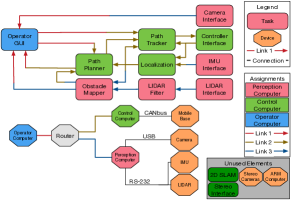
Figure 1: Example teleoperated robot for the system synthesis problem. The top graph represents a generic software graph for this problem, while the bottom graph represents a generic hardware graph.

III-A Task Assignment And Routing

In order to rigorously describe a complex robotic system, we begin by defining a few basic concepts. A multiset is a collection of $I$ objects $\Psi=\{\psi_{i}\;|\;i=1,\ldots,I\}$, in which a given object may occur more than once in the collection. The indicator function $\mathbbm{1}_{\psi_{i}}(\Psi):\Psi\rightarrow[1,\infty)$ defines the number of times an object $\psi_{i}$ occurs in $\Psi$. A set is the special case of a multiset in which every object occurs only once, $\mathbbm{1}_{\psi_{i}}(\Psi)=1\;\forall\;\psi_{i}\in\Psi$. A graph $\mathcal{G}=(V,E)$ is defined by a set of vertices $V=\{v_{i}\;|\;i=1,\ldots,I\}$, and a multiset of edges $E=\{e_{i}=\{v_{i},v_{j}\}\;|\;v_{i},v_{j}\in V\}$ which connect pairs of vertices. The vertices participating in edge $e_{i}$ are indexed in the form $e_{i,n}\;|\;n=1,2$, also known as a loop if $e_{i,1}=e_{i,2}$. Restrictions on the set of edges $E$ define several important classes of graphs which will be used throughout this paper: a simple graph possesses a set of edges $E$ in which no edge is a loop; a multigraph possesses a multiset $E$ with no loops; and a pseudograph possesses a multiset $E$ possibly with loops. Additionally, if the order of vertices in edges is fixed, this defines a directed graph, otherwise a graph may be referred to as an undirected graph. Figure 2 provides examples of each graph type to demonstrate their fundamental differences. In this work, graph is used to describe the case in which no assumptions are made about the nature of the graph, with more specific terms used when additional constraints hold true. Furthermore, in order to disambiguate discussions between hardware and software graph elements, hardware vertices and edges are referred to as devices and connections, while software vertices and edges are referred to as tasks and links.

(a) Simple, Undirected Graph

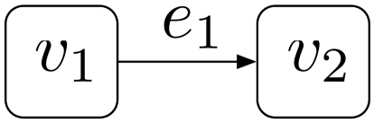
(b) Simple, Directed Graph

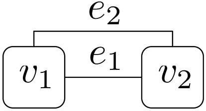
(c) Multigraph

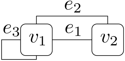
(d) Pseudograph

Figure 2: Example graphs.

Hardware and software elements form the basis from which a system can be composed. Consider a system consisting of two graphs representing the hardware and software aspects of a system. The set $\Pi=\{\pi_{d}\;|\;d=1,\ldots,D\}$ defines the $D$ devices in the hardware graph, which provide computational resources and connections to other devices. Each device $\pi_{d}$ can provide computational resources for executing tasks, although given the heterogeneous nature of devices, not every device may provide every resource. The entire system contains $W$ possible resources, so for every device $\pi_{d}$, a vector $\vec{r}_{\pi_{d}}=\langle r_{\pi_{d},w}\;|\;w=1,\ldots,W;r_{\pi_{d},w}\in[0,\infty)\rangle$ defines the resources available on device $\pi_{d}$. These resources represent computational resources such as available processing power, RAM, disk storage, or logical access to particular peripherals. The multiset of edges $\Gamma=\left\{\gamma_{k}=\left\{\pi_{u},\pi_{v}\right\}\;|\;k=1,\ldots,K;\pi_{u},\pi_{v}\in\Pi\right\}$ define the connections between devices which can support data transmission. Note that this allows multiple connections between devices, since devices can be connected to each other via differing physical transports (e.g. both USB and ethernet) or various forms of internal communication (e.g. shared memory or a loopback interface). Connections provide finite bandwidth for transmitting data, resulting in a set of bandwidth limits $B=\{b_{\gamma_{k}}\;|\;\gamma_{k}\in\Gamma;b_{\gamma_{k}}\in[0,\infty)\}$. The set of devices and connections define the hardware pseudograph $\mathcal{H}=(\Pi,\Gamma)$, which provides computational resources for executing tasks, and connectivity for transferring data. To visualize how these parameters relate to a hardware pseudograph, consider the simple example in Figure 3, which demonstrates each of these parameters with a subset of Figure 1.

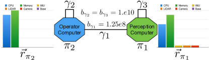
Figure 3: Simple example of a hardware pseudograph and relevant parameters.

In parallel to the hardware pseudograph, the set $T=\{\tau_{p}\;|\;p=1,\ldots,P\}$ defines the $P$ tasks in the software graph, which perform the computational work. Tasks may consume computational resources, process and publish data, and interface with sensors and actuators, therefore a device is required to provide these resources for task execution. The resources required for a particular task may vary between devices, e.g. due to hardware specialization, where the resources consumed by a task $\tau_{p}$ executing on device $\pi_{d}$ is denoted by the vector $\vec{c}_{\pi_{d}}^{\,\tau_{p}}=\langle c_{\pi_{d},w}^{\tau_{p}}\;|\;w=1,\ldots,W;c_{\pi_{d},w}^{\tau_{p}}\in[0,\infty]\rangle$. The multiset of $L$ edges $\Lambda=\{\lambda_{l}=\{\tau_{o},\tau_{i}\}\;|\;l=1,\ldots,L;\tau_{o},\tau_{i}\in T,\tau_{o}\neq\tau_{i}\}$ models the links that transmit data necessary for operation, and the output of computation used by other tasks. Unlike the hardware pseudograph, the edge multiset $\Lambda$ does not contain self-loops since tasks have internal access to generated data. This restriction yields a software multigraph defined as $\mathcal{S}=(T,\Lambda)$, an example of which is given in Figure 4.

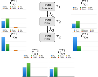
Figure 4: Simple example of a software multigraph and relevant parameters.

In order to define a complete computational system, there must also exist a mapping $\alpha_{\mathcal{H}}^{\mathcal{S}}:\mathcal{S}\rightarrow\mathcal{H}$, which defines how software executes on the specified hardware. A computational system is defined in this work as $\mathcal{R}=\{\mathcal{H},\mathcal{S},\alpha_{\mathcal{H}}^{\mathcal{S}}\}$, a set containing the hardware graph, software graph, and the assignment mapping. An assignment variable $\alpha_{\pi_{d}}^{\tau_{p}}\in\{0,1\}$ defines whether task $\tau_{p}$ executes on device $\pi_{d}$. Assignments must be binary and atomic, meaning a task $\tau_{p}$ executes on one and only one device $\pi_{d}\in\Pi$, as represented in Equation 1c. The consumption of computational resources by tasks cannot over-allocate device budgets, resulting in Equation 1e. In addition to tasks consuming computational resources, transmitting data between tasks consumes bandwidth on hardware connections. The transfer of data between two connected tasks consumes bandwidth traversing a connection, with link $\lambda_{l}$ consuming $c_{\gamma_{k}}^{\lambda_{l}}$ worth of bandwidth over connection $\gamma_{k}$. The amount of bandwidth consumed can vary due to the differences in connections (e.g., packetized network overhead, requirements on data representations, etc.), requiring the bandwidth utilization to take the connection $\gamma_{k}$ into account as well. A link $\lambda_{l}$ may be assigned to transmit over a connection $\gamma_{k}$, denoted by the variable $\alpha_{\gamma_{k}}^{\lambda_{l}}\in\{0,1\}$, which consumes the specified amount of bandwidth $c_{\gamma_{k}}^{\lambda_{l}}$. Equation 1f ensures that the assignment of links to connections respects the bandwidth limits specified previously. Tasks may be assigned to devices not directly connected to one another, requiring data routing along multiple connections. Multi-hop paths require routing data along a connected path between the devices assigned to each task. LABEL:eqn:flow ensures these properties for all routes with a flow constraint stating that for any device interacting with a link, it must have either an odd number of connections and assigned to the relevant device (e.g., a source or sink) or an even number of connections transmitting the data (e.g., uninvolved or flowing through). This logic is formulated on a per-link basis to ensure a linear constraint, and is visualized in Figure 5, where $\gamma_{k,\cdot}$ and $\lambda_{l,\cdot}$ represent the indexed element (device or task) participating in the edge, and $E(\cdot)$ represents the edges adjacent to a given element.

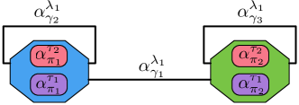
Figure 5: Example flow constraints. Any attempt to trace from an assignment of $\tau_{1}$ to an assignment of $\tau_{2}$ will result in satisfying the flow constraint.

The constraints described to this point are analogous to those in the multi-resource quadratic routing and assignment problem [19]. However, we point out that we have reformulated the problem in a graph-theoretic manner to allow later for optimizing the hardware and software graph structures. Next, consider two functions (either linear or quadratic), $f_{exec}:(\Pi,T)\rightarrow\mathbb{R}$ and $f_{route}:(\Gamma,\Lambda)\rightarrow\mathbb{R}$ defining the cost of each assignment, used to generate the cost function for considering a particular $\alpha_{\mathcal{H}}^{\mathcal{S}}$. Writing this as a constrained minimization aims to find an optimal mapping for the given computational system, as seen in Equation 1.

$$\begin{split}Z=\mathtt{min}&\sum_{\tau_{p}\in T}\sum_{\pi_{d}\in\Pi}\alpha_{\pi_{d}}^{\tau_{p}}f_{exec}(\pi_{d},\tau_{p})+\\ &\sum_{\gamma_{k}\in\Gamma}\sum_{\lambda_{l}\in\Lambda}\alpha_{\gamma_{k}}^{\lambda_{l}}f_{route}(\gamma_{k},\lambda_{l})\end{split}$$ (1a)

s.t.

$$\begin{split}\sum_{\pi_{d}\in\Pi}\alpha_{\pi_{d}}^{\tau_{p}}=1\quad\forall\;\tau_{p}\in T\end{split}$$ (1c)

$$\begin{split}\alpha_{\gamma_{k,1}}^{\lambda_{l,1}}+\sum_{\gamma_{i}\in E(\gamma_{k,1})}&\alpha_{\gamma_{i}}^{\lambda_{l}}=\alpha_{\gamma_{k,2}}^{\lambda_{l,2}}+\sum_{\gamma_{o}\in E(\gamma_{k,2})}\alpha_{\gamma_{k}}^{\lambda_{l}}\\ &\forall\;\lambda_{l}\in\Lambda;\gamma_{k}\in\Gamma\\ \end{split}$$ (1d)

$$\sum_{\tau_{p}\in T}\alpha_{\pi_{d}}^{\tau_{p}}c_{\pi_{d},w}^{\tau_{p}}\leq r_{\pi_{d},w}\quad\forall\;\pi_{d}\in\Pi;w=1,\ldots,W$$ (1e)

$$\sum_{\lambda_{l}\in\Lambda}\alpha_{\gamma_{k}}^{\lambda_{l}}d_{\gamma_{k}}^{\lambda_{l}}\leq b_{\gamma_{k}}\quad\forall\;\gamma_{k}\in\Gamma$$ (1f)

III-B Structure Synthesis

Previous works accept the hardware and software graphs, $\mathcal{H}$ and $\mathcal{S}$, as the input to the optimization problem. A key contribution in this paper is to generalize the optimization problem (1) to instead accept as input the sets of available hardware $\Pi$ and software $T$, enabling synthesis of hardware and software structures in finding an optimal computational system $\mathcal{R}$. Additional constraints must be introduced to ensure the graph structure produces a system with two key properties: consistency and viability. Consistency requires that the assignment variables represent a physically realizable system - devices cannot connect to non-existent devices, tasks cannot send or receive data from inactive tasks, and so forth. Viability ensures that the synthesized graphs support the requirements of all constituent elements, while still respecting the assignment and routing constraints described in subsection III-A. For instance, any generated hardware pseudograph must provide the necessary resources to support execution of the software multigraph; devices must have sufficient resources to support task execution, and the connections between devices must provide enough bandwidth for transferring data between tasks. Viability addresses only local concerns in generating graphs (e.g. ensuring devices can connect to one another, tasks have required resources and data inputs, etc.), deferring the treatment of systemic functionality to later constraints. These consistency and viability concepts underlie the novel constraints which enable expanding task assignment and routing to include the synthesis of hardware and software graphs.

The first step in generating the hardware pseudograph requires generalizing to all possible configurations of devices and connections. The set of devices $\Pi$ can be trivially re-interpreted as the set of devices under consideration for inclusion. In place of explicit device connections $\Gamma$ as an input defined previously, each device instead defines a capacity for number of connections for each physical transport type. Considering all possible devices in a given system, there exists $X$ distinct physical transport types, allowing the definition of a connection capacity vector $\vec{\chi}_{\pi_{d}}=\langle\chi_{\pi_{d},x}\;|\;x=1,\ldots,X;\chi_{\pi_{d},x}\in[0,\infty)\rangle$ for each device. Given $D$ devices under consideration, the set of possible connections between devices in the pseudograph given a single physical transport can be defined as $\Gamma_{x}=\{\gamma_{x,k}=\{\pi_{u},\pi_{v}\}\;|\;k\in E(K_{D});\pi_{u},\pi_{v}\in\Pi\}$, where $E(K_{D})$ denotes the edges in a complete graph with $D$ vertices. This redefines the multiset of connections as the union of possible connections for each transport type, $\Gamma=\bigcup_{x=1}^{X}\;\Gamma_{x}$. For convenience, $\gamma_{x,k}$ represents the $k$-th potential connection using the $x$-th transport type. With these definitions for vertices and edges, the hardware pseudograph now represents all possible graphs given the redefined vertices and edges, allowing assignment variables to select one specific instance. A device selection variable $\alpha_{\pi_{d}}\in\{0,1\}$ represents the decision to include the $d$-th device in the final system. These variables form a unique basis in this formulation, in that a device has no external requirements for viability. Devices are assumed to not depend on other devices, and do not require connections to other devices in order to operate.

Remark.

The resource provision/consumption constraints required to relax the above assumption are identical in form to those used to represent the provision/consumption of resources for software tasks. This relaxation is not included in this formulation in order to focus on hardware supporting software.

Selected devices still must provide the computational resources necessary for task execution as defined in Equation 1e, with constraint on local budgets being sufficient for ensuring global resource needs are met. The assignment variable $\alpha_{\gamma_{x,k}}\in\{0,1\}$ selects a particular connection between two devices. Consistent connections respect the fact that a connection can only occur between two selected devices, producing Equation 2. Viable connections must not exceed the connection capacities defined for any device, resulting in Equation 3.

$$\alpha_{\pi_{d}}\geq\alpha_{\gamma_{x,k}}\quad\forall\;\pi_{d}\in\Pi;\gamma_{x,k}\in E(\pi_{d})$$ (2)

$$\sum_{\gamma_{x,k}\in E(\pi_{d},x)}\alpha_{\gamma_{x,k}}\leq\chi_{\pi_{d},x}\quad\forall\;\pi_{d}\in\Pi;x=1,\ldots,X$$ (3)

Introducing flexibility in device connections separates two previously intertwined concepts: data connection, and logical device access. A task may operate as a device driver, which requires both access to a specific physical transport (e.g. CANbus), as well as logical access to a particular device (e.g. a particular motor controller) over that transport. Previously, a device driver task would consume resources combining both concepts, while the computing device connected to the relevant peripheral offering the matching resource. This allowed simplifying the problem to a tightly-coupled resource model, in which the resource budget only considers the device providing resources. While these resources are still considered as the set of $W$ resources available in a given problem, we now consider the resources provided by a particular connection, represented as $\vec{r}_{\gamma_{x,k}}=\langle r_{x,k,j}\;|\;j=1,\ldots,J\rangle$. This reformulates the resource budget constraints Equation 1e to introduce these link-level resources, as shown in Equation 4.

$$\begin{split}\sum_{\tau_{p}\in T}\alpha_{\pi_{d}}^{\tau_{p}}c_{\pi_{d},j}^{\tau_{p}}&\leq r_{\pi_{d},j}+\sum_{\gamma_{x,k}\in\Gamma}\alpha_{\gamma_{x,k}}r_{x,k,j}\\ &\forall\;\pi_{d}\in\Pi;j=1,\ldots,J\end{split}$$ (4)

The augmented resource budget provides viability during task assignment, ensuring the correct accounting for tasks interfacing to peripheral devices for operation. This formulation enables the generation of a hardware pseudograph as a necessary component for the software multigraph.

In the example in Figure 6, the base computer interfacing with an IMU has been broken into two separate devices, the computer and the IMU, respectively. The original graph has been decomposed into individual elements with capacities defined for generating hardware pseudographs. Connecting to the IMU over RS–232 requires the IMU to exist in the final assignment as a logical consequence of this decomposition. Logical access to the IMU no longer exists as a computational resource for the base computer, instead being available as a resource for connecting to the IMU via RS–232.

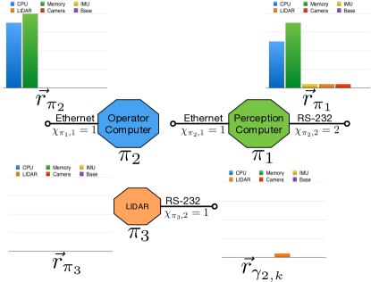
Figure 6: Example device generalization for system synthesis.

Generalizing the software multigraph requires slightly different relaxations due to the atomic nature of task assignment. The set of assignment variables for an individual task can be interpreted as both assigning a task to some device and describing the set of possible tasks. Modifying Equation 1c accomplishes this by allowing a task to remain unassigned to any device, and thus unused, as seen in Equation 5.

$$\sum_{\pi_{d}\in\Pi}\alpha_{\pi_{d}}^{\tau_{p}}\leq 1\quad\forall\;\tau_{p}\in T$$ (5)

While previous requirements for task assignment still hold in task assignment for computational resources, new requirements exist for the links between tasks. Tasks define some number of outputs which produce data, and some number of inputs which accept data for processing. A task $\tau_{p}\in T$ defines $O_{\tau_{p}}$ available outputs in the set $\Omega_{\tau_{p}}=\{\omega_{\tau_{p},o}\;|\;o=1,\ldots,O_{\tau_{p}}\}$, and $I_{\tau_{p}}$ required inputs in the set $\Xi_{\tau_{p}}=\{\xi_{\tau_{p},i}\;|\;i=1,\ldots,I_{\tau_{p}}\}$. A task then can provide a set of possible links $\Lambda_{\tau_{p}}\subset\{\lambda_{\tau_{p},\tau_{r},\omega_{\tau_{p},o},\xi_{\tau_{r},i}}\;|\;\tau_{p},\tau_{r}\in T,\tau_{p}\neq\tau_{r};\omega_{\tau_{p},o}\in\Omega_{\tau_{p}};\xi_{\tau_{r},i}\in\Xi_{\tau_{r}}\}$ defining all possible outgoing links from $\tau_{p}$, where all possible links in the software multigraph are defined as $\Lambda=\bigcup_{\tau_{p}\in T}\Lambda_{\tau_{p}}=\{\lambda_{l}\;|\;1,\ldots,L\}$. Note that the set of possible links any output may provide is a subset of all possible combinations of inputs and outputs, unlike the definition of connections between devices.

Data transmitted in software systems require agreement on typing or structure of data, analogous to physical transports for device connections. We define functions $f_{intype}:\Omega\rightarrow[0,\infty)$ and $f_{outtype}:\Xi\rightarrow[0,\infty)$, which map possible link structures to a number uniquely associated with each message type. Valid transmission of data between tasks only occurs when the type on both sides agree, leading to Equation 6 below.

$$\alpha_{\lambda_{l}}f_{intype}(\lambda_{l,1})=\alpha_{\lambda_{l}}f_{outtype}(\lambda_{l,2})\quad\forall\lambda_{l}\in\Lambda$$ (6)

Unlike device connections, there exists no fundamental limit on the number of links active to a given input, eliminating the need to use a budgetary constraint to limit the number of possible links. While connections between devices provide the capability for transferring data, links between tasks actualize the transfer. For each link, $\alpha_{\lambda_{l}}\in\{0,1\}$ represents the decision to transfer data from one task’s output to another task’s input. All inputs for an active task must have at least one output linked to provide data, but unlike physical connections, no fundamental limit exists on the number of outputs linked to a single input. This allows aggregation of data for processing, leading to a satisfaction constraint in Equation 7 applying to each task input. The previously defined variable $\alpha_{\gamma_{k}}^{\lambda_{l}}$ maintains the original interpretation of assigning a link to a particular connection, with an additional constraint ensuring the assignment of links to active connections only in Equation 8.

$$\sum_{\pi_{d}\in\Pi}\alpha_{\pi_{d}}^{\tau_{p}}\leq\sum_{\lambda_{l}\in\Xi_{\tau_{p}}}\alpha_{\lambda_{l}}\quad\forall\;\tau_{p}\in T$$ (7)

$$\alpha_{\gamma_{k}}^{\lambda_{l}}\geq\alpha_{\lambda_{l}}\quad\forall\;\lambda_{l}\in\Lambda;\gamma_{k}\in\Gamma$$ (8)

Beyond data typing, inputs and outputs in the software multigraph may provide different semantic meaning representing some underlying assumption of a task. For instance, an output transmitting a pose message may contain the estimated pose of a robot, the sensed location of an object of interest, or a commanded goal pose. These instances share a common data type, but represent different quantities in the software system. In order to ensure that the structure keeps semantic consistency, outputs define a vector of $W_{\omega_{o}}$ “resources” $\vec{r}_{\omega_{o}}=\langle r_{\omega_{o},w}\;|\;w=1,\ldots,W_{\omega_{o}};r_{\omega_{o},w}\in[0,\infty)\rangle$ which represent the semantic content provided by this output. Similarly, inputs define a vector of $W_{\xi_{i}}$ requirements $\vec{c}_{\xi_{i}}=\langle c_{\xi_{i},w}\;|\;w=1,\ldots,W_{\xi_{i}};c_{\xi_{i},w}\in[0,\infty)\rangle$ representing the required semantic content for a given input. In addition to active tasks requiring all inputs have at least one assigned link, the assigned links must satisfy the defined budget, as seen in Equation 9. An example of the semantic budget/consumption for links can be seen in Figure 7, in which all two outputs and two inputs work with an identical LIDAR data structure, but semantically different meanings (e.g. raw or ego-filtered data). These constraints also introduce inconsistencies in the routing constraints in LABEL:eqn:flow - tasks may not send data to all potential recipients due to semantic requirements. Equation 10 introduces the link assignment variable into the original constraint such that the constraint only applies to the active links. This introduces a quadratic constraint, which can be linearized by introducing a dummy variable, $\alpha_{\varnothing\pi_{d}}^{\tau_{p}}\in\{0,1\}$, for each task assignment, which balances the constraint when tasks are utilized but not linked, as seen in Equation 11. The linear form of this constraint is not used due to poor performance, but is included to demonstrate a formulation with purely linear constraints.

$$\sum_{\lambda_{l}\in\Xi_{\tau_{p}}}\alpha_{\lambda_{l}}r_{\lambda_{l,1},j}\geq c_{\xi_{i},j}\quad\forall\;\tau_{p}\in T;\xi_{i}\in\Xi_{\tau_{p}};j=1,\ldots,W_{\xi_{i}}$$ (9)

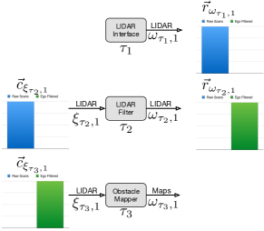
Figure 7: Example task generalization. While all inputs and outputs share the same structure, semantic content differs them.

$$\begin{split}\alpha_{\lambda_{l}}(\alpha_{\lambda_{l,1}}^{\gamma_{k,1}}+\sum_{\gamma_{i}\in E(\gamma_{k,1})}&\alpha_{\gamma_{i}}^{\lambda_{l}})=\alpha_{\lambda_{l}}(\alpha_{\lambda_{l,2}}^{\gamma_{k,2}}+\sum_{\gamma_{o}\in E(\gamma_{k,2})}\alpha_{\gamma_{o}}^{\lambda_{l}})\\ &\forall\;\lambda_{l}\in\Lambda;\gamma_{k}\in\Gamma\end{split}$$ (10)

$$\begin{split}\frac{\alpha_{\lambda_{l,1}}^{\gamma_{k,1}}+\alpha_{\varnothing\lambda_{l,1}}^{\gamma_{k,1}}}{2}+\sum_{\gamma_{i}\in E(\gamma_{k,1})}&\alpha_{\gamma_{i}}^{\lambda_{l}}=\frac{\alpha_{\lambda_{l,2}}^{\gamma_{k,2}}+\alpha_{\varnothing\lambda_{l,2}}^{\gamma_{k,2}}}{2}+\sum_{\gamma_{o}\in E(\gamma_{k,2})}\alpha_{\gamma_{o}}^{\lambda_{l}}\\ &\forall\;\lambda_{l}\in\Lambda;\gamma_{k}\in\Gamma\end{split}$$ (11)

Besides the new constraints of the software multigraph, consistency introduces a few additional constraints on task assignment. With the introduction of inactive devices, tasks can only execute on devices participating in the system (Equation 12), and a link can only route over active connections (Equation 13).

$$\alpha_{\pi_{d}}^{\tau_{p}}\leq\alpha_{\pi_{d}}\quad\forall\;\pi_{d}\in\Pi;\tau_{p}\in T$$ (12)

$$\alpha_{\gamma_{k}}^{\lambda_{l}}\leq\alpha_{\gamma_{k}}\quad\forall\;\gamma_{k}\in\Gamma;\lambda_{l}\in\Lambda$$ (13)

These constraints ensure selected graph structures maintain consistency in the overall system, and viability during assignment. Combined with the previous constraints for task assignment and routing, any system adhering to these constraints supports the operation of every element.

III-C Context-Aware Functional Modularity

The constraints presented thus far provide a method for composing a computational system from a list of available elements, without regard for the overall functionality of the system. In order to generate systems with desired functionality, a problem definition requires a description of the desired system functionality, and a framework for determining the contributions subsets of the system provide. Functionality is assumed to be "linearly independent", in the sense that system requirements can be met by summing functionality from system components. Given the complexity of functional decomposition already present in robotic systems, and the interaction between robots and their environment, two additional notions are introduced to define functional capabilities. First, system functionality is defined as two separate components, mission parameters, and mission context, which define functional requirements and the conditions under which the system must operate to provide those requirements. Second, functionality is provided to a system through collections of components referred to as modules. These two additions serve to address some of the real world complexities present in determining functional capabilities.

As an example, consider a mission parameter for a hypothetical robot that specifies the ability to localize the robot within the environment during operation. Many possible approaches for robot localization exist [34, 35, 36, 37], varying in input data, computational complexity, and underlying theory of operation. However, many approaches vary in the assumptions made about the environment, robot, or mission under which the approach will operate; GPS-based localization approaches assume direct visibility of the sky, Kinect-based localization requires indoor environments for the sensor to receive usable data, and 2D localization approaches assume a planar environment. Let these assumptions compose a vector of $J$ elements defining the mission context $\vec{s}=\langle s_{j}\;|\;j=1,\ldots,J;s_{j}\in[0,\infty)\rangle$. The task definition is then augmented with a vector $\vec{y}_{\tau_{p}}=\langle y_{j}\;|\;j=1,\ldots,J;y_{j}\in[0,\infty)\rangle$ defining the context required for a task to execute. In this way, $\vec{x}$ defines a $J$-dimensional bounding box inside which tasks must exist in order to correctly execute, representing the underlying assumptions about the environment a task encodes. This bounding box generates a contextual constraint in Equation 14 to ensure that no task executes in an invalid context.

$$\sum_{\pi_{d}\in\Pi}\alpha_{\pi_{d}}^{\tau_{p}}y_{\tau_{d},j}\leq s_{j}\quad\forall\;\tau_{d}\in T;j=1,\ldots,J$$ (14)

If the mission context includes both outdoor and planar world assumptions, GPS and 2D localization techniques can operate, while indoor-only techniques cannot. When combined with previous constraints, functionality exists when tasks can execute under the correct set of environmental assumptions, with the necessary computational resources, and attached to the appropriate hardware.

Derived as an instance of an assignment problem, the entire problem has been cast in terms of constraints on individual decisions related to the tasks and devices composing the system. This approach dovetails with the approach taken by many modern robotics software systems, which present tasks as the unit of functionality and reuse [5, 38, 39]. Tasks provide an intuitive unit of functionally reusable software in this context for a variety of reasons: tasks provide a simple model of usability (inputs, process, outputs), require minimal effort to use (launch task, provide data), and can naturally isolate development of novel algorithms. Tying reusability to an individual executable black box presents a problem when considered across an ecosystem consisting of diverse contributions. Reusability tends to favor smaller units of modularity [40], exerting downward pressure to produce tasks with compact sets of functionality. However, the definition of functional completeness for an individual task varies between different approaches, depending on performance considerations, underlying algorithms, or philosophical views. Tasks thus define functional scope differently depending on the individual resolution of this tension, breaking the direct coupling between task selection and functional capability. Depending on the decomposition of functionality in a given problem, some units of functionality will inevitably require more than a single task to implement. In order to introduce functionality requirements, this work introduces a mid-level concept of functional modules.

A module represents a collection of tasks and devices which, if included in a computational system, provide some amount of functionality to the overall system. This provides an abstraction through which an expert can normalize functionality metrics over a set of options, as well as provide any simplifying constraints on the structure of a particular subsystem. With structure synthesis, the problem input defines a set of tasks $T$, and a set of devices $\Pi$; modularity partitions these sets into $N$ disjoint subsets. Thus, a module $\mu$ is defined by the set of tasks $T_{\mu}=\{\tau_{p}\;|\;p=1,\ldots,P_{\mu}\}$ and the set of devices $\Pi_{\mu}=\{\pi_{d}\;|\;d=1,\ldots,D_{\mu}\}$. The full set of modules can then be written $M=\{\mu_{n}=\{\Pi_{\mu},T_{\mu}\}\;|\;n=1,\ldots,N\}$, with the example elements organized into modules in Figure 8. By definition, a module only functions for systems including all elements, which introduces an atomicity relationship between all elements and each individual task (Equation 15) and device (Equation 16). Functionality is defined by $Q$ functional requirements possible in a given problem, with a valid system requiring $\vec{r}_{s}=\langle r_{s,q}\;|\;q=1,\ldots,Q;r_{q}\in[0,\infty)\rangle$. Modules provide functional capabilities $\vec{c}_{\mu}=\langle c_{\mu,q}\;|\;q=1,\ldots,Q;c_{\mu,q}\in[0,\infty)\rangle$ if selected. While a new assignment variable, $\alpha_{\mu}$, could be introduced to indicate the selection of a particular module, this variable can be represented in terms of the assignment of component elements. To minimize the number of variables in the formulation, the indicator function in Equation 17 will be used, although the formulation will continue to use $\alpha_{\mu}$ for brevity. The sum of the functionality vectors of active modules must meet or exceed the mission parameters $\vec{r}_{s}$, resulting in the final constraint on mission readiness in Equation 18.

$$\begin{split}(D_{\mu}+P_{\mu})&\sum_{\pi_{d}\in\Pi}\alpha_{\pi_{d}}^{\tau_{p}}=\sum_{\pi_{d}\in\Pi_{\mu}}\alpha_{\pi_{d}}+\sum_{\tau_{r}\in T_{\mu}}\sum_{\pi_{d}\in\Pi}\alpha_{\pi_{d}}^{\tau_{r}}\\ &\forall\;\mu\in M;\tau_{p}\in T_{\mu}\end{split}$$ (15)

$$\begin{split}(D_{\mu}+P_{\mu})\alpha_{\pi_{d}}&=\sum_{\pi_{r}\in\Pi_{m}}\alpha_{\pi_{r}}+\sum_{\tau_{d}\in T_{m}}\sum_{\pi_{r}\in\Pi}\alpha_{\pi_{r}}^{\tau_{d}}\\ &\forall\;\mu\in M;\pi_{d}\in\Pi_{\mu}\end{split}$$ (16)

$$\alpha_{\mu}=\frac{\sum_{\pi_{d}\in\Pi_{\mu}}\alpha_{\pi_{d}}+\sum_{\tau_{d}\in T_{\mu}}\sum_{\pi_{d}\in\Pi}\alpha_{\pi_{d}}^{\tau_{p}}missing}{D_{\mu}+P_{\mu}}$$ (17)

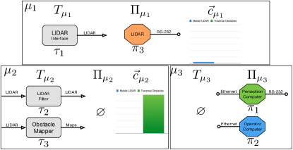
Figure 8: Example tasks organized into modules. Requiring Traversal Obstacles from $\mu_{2}$ requires all three modules to fully satisfy constraints.

$$\sum_{\mu\in M}\alpha_{\mu}c_{\mu,q}\geq r_{s,q}\quad\forall\;q=1,\ldots,Q$$ (18)

Allowing functionality metrics to be compared directly at the module level enables reasoning about the opportunity costs in a system design, since assignment can begin to reason about the tradeoffs in selecting one module over another, similar to a trade study performed by an expert. Crucially, modules only contain elements directly related to the defined functional capabilities, but not necessarily all elements required to produce a complete system. This functional independence, combined with previous constraints, introduces automatic dependency resolution among modules - selecting one module may require the selection of other modules to produce a complete system. The variable scale of modules and functionality capability in modules, combined with the assurance that the resulting system ensures a complete system, allows for applying this approach to a wide range of system synthesis problems. Modules can represent small, single function components, building to a larger individual robot as easily as they can represent individual pre-built robots composing a complex multi-robot system. Thus, this extension serves to unify design for a wide range of robotic systems.

III-D Objective Function and Full Formulation

As a constrained minimization problem, combining the constraints defined previously with an objective function completes the formulation for selecting an optimal system. These cost functions can be defined in a variety of ways, depending on the desired metrics to define an optimal system. The cost function is presented in a generalized fashion to enable a point by which expert knowledge can be applied to define optimality for a given scenario. Similar to the MRQARP, the full objective function can be composed from a set of functions considering the assignment operations present in the problem definition. For system synthesis, these functions are augmented with additional functions to consider the three additional assignments: modules, devices, and connections. The overall objective function in Equation 20 composes the overall cost function from terms representing the user defined costs for each selection.

As a higher level organizational structure, modules offer the most complex function for determining cost. The cost for selecting a module is defined as the sum of costs for each constituent device, as well as a subsystem cost for selecting the module independent of its constituent elements. Both device-specific and module-specific costs are independent of other elements of the system, since they are not embedded in some other aspect of the system. These functions are combined to produce the total cost function in Equation 19. For each device, $f_{dev}:\Pi\rightarrow\mathbb{R}$, represents the cost of including a given device and a cost representing any overhead for utilizing a module, $f_{o}:M\rightarrow\mathbb{R}$.

$$\begin{split}f_{m}=(f_{o}(\mu)+\sum_{\pi_{d}\in\Pi_{\mu}}f_{dev}(\pi_{d}))\end{split}$$ (19)

Task costs result from resource consumption as a result of execution, requiring consideration of the device assignment, and thus are considered independent of module selection. The cost function for task execution is identical to the one defined for Equation 1, with the same considerations. Device connection costs of the form $f_{cnx}:\Gamma\rightarrow\mathbb{R}$ not only serve the previously stated system goals, but also serve to handle physicality constraints on system components. Assigning infinite costs to physical connections between devices (e.g. wired connections) ensures that connections between devices cannot imose unwanted physical connections. Common cases for this need include remote operator stations, in which a robot needs to transmit data without constraining motion, or multi-robot systems, in which individual robots must remain physically independent. Message routing introduces costs for utilizing bandwidth available on device connections, which aims to reduce latency. The particulars of modeling latency in networks are beyond the scope of this problem formulation, but instead, the intuition that an oversubscribed connection will result in delivery time increasing unbounded with time serves to motivate that reducing bandwidth utilization will minimize latency. The relationship between bandwidth utilization and latency can vary depending on the devices connected, the physical transport connecting them, and the link routed over a particular connection. This function is identical to $f_{route}$ defined previously. Note that while these two costs are logically separate, the cost function in Equation 20 combines them in a slightly more concise form, in which the message routing cost computation is included as a term in the device connection equation. These functions are combined to produce the total system cost function in Equation 20a.

The selection of the sub-functions not only sets the metrics by which possible systems are compared, but also defines the complexity of the given problem. If all functions $f$ are linear functions, the final problem is formulated as an integer linear program; if any function is quadratic, the problem is instead a quadratic program. As an example, task costs can be quantified by linear metrics (e.g. resource utilization) or quadratic metrics (e.g. load balancing, power utilization, thermal load). In order to demonstrate the overall capability of system synthesis to construct optimal systems, the remainder of this work will assume linear functions, and thus an integer linear program. While many other frameworks exist for solving this type of constrained optimization (e.g. guided local search, genetic algorithms, simulated annealing), an integer linear program can be solved for the global optimum, demonstrating the optimal solution and worst case in performance. This problem represents a generalization of the (MRQARP) [19], which has been proven to be $\mathcal{NP}$-hard in the strong sense [41]. The additional variables representing the structure of the graphs and functional requirements can be set to trivial values such that a problem instance maps to an instance of MRQARP, leading this problem to share the same complexity class.

$$\begin{split}Z=\mathtt{min}&\sum_{\mu\in M}\left(\alpha_{\mu}\left(f_{o}(\mu)+\sum_{\pi_{d}\in\Pi_{\mu}}f_{dev}(\pi_{d})\right)\right)+\\ &\sum_{\tau_{p}\in T}\sum_{\pi_{d}\in\Pi}\alpha_{\pi_{d}}^{\tau_{d}}f_{exec}(\pi_{d},\tau_{p})+\\ &\sum_{\gamma_{k}\in\Gamma}\left(\alpha_{\gamma_{k}}f_{cnx}(\gamma_{k})+\sum_{\lambda_{l}\in\Lambda}\alpha_{\gamma_{k}}^{\lambda_{l}}f_{route}(\gamma_{k},\lambda_{l})\right)\end{split}$$ (20a)

s.t.

$$\sum_{\mu\in M}\alpha_{\mu}c_{\mu,q}\geq r_{s,q}\quad\forall\;q=1,\ldots,Q$$ (20c)

$$\sum_{\pi_{d}\in\Pi}\alpha_{\pi_{d}}^{\tau_{p}}y_{\tau_{d},j}\leq s_{j}\quad\forall\;\tau_{d}\in T;j=1,\ldots,J$$ (20d)

$$\begin{split}(D_{\mu}+P_{\mu})&\sum_{\pi_{d}\in\Pi}\alpha_{\pi_{d}}^{\tau_{p}}=\sum_{\pi_{d}\in\Pi_{\mu}}\alpha_{\pi_{d}}+\sum_{\tau_{r}\in T_{\mu}}\sum_{\pi_{d}\in\Pi}\alpha_{\pi_{d}}^{\tau_{r}}\\ &\forall\;\mu\in M;\tau_{p}\in T_{\mu}\end{split}$$ (20e)

$$\begin{split}(D_{\mu}+P_{\mu})\alpha_{\pi_{d}}&=\sum_{\pi_{r}\in\Pi_{\mu}}\alpha_{\pi_{r}}+\sum_{\tau_{d}\in T_{\mu}}\sum_{\pi_{r}\in\Pi}\alpha_{\pi_{r}}^{\tau_{d}}\\ &\forall\;\mu\in M;\pi_{d}\in\Pi_{\mu}\end{split}$$ (20f)

$$\alpha_{\gamma_{k}}^{\lambda_{l}}\leq\alpha_{\gamma_{k}}\quad\forall\;\gamma_{k}\in\Gamma;\lambda_{l}\in\Lambda$$ (20g)

$$\alpha_{\pi_{d}}^{\tau_{p}}\leq\alpha_{\pi_{d}}\quad\forall\;\pi_{d}\in\Pi,\tau_{p}\in T$$ (20h)

$$\alpha_{\lambda_{l}}f_{intype}(\lambda_{l,1})=\alpha_{\lambda_{l}}f_{outtype}(\lambda_{l,2})\quad\forall\lambda_{l}\in\Lambda$$ (20i)

$$\begin{split}\alpha_{\lambda_{l}}(\alpha_{\lambda_{l,1}}^{\gamma_{k,1}}+\sum_{\gamma_{i}\in E(\gamma_{k,1})}&\alpha_{\gamma_{i}}^{\lambda_{l}})=\alpha_{\lambda_{l}}(\alpha_{\lambda_{l,2}}^{\gamma_{k,2}}+\sum_{\gamma_{o}\in E(\gamma_{k,2})}\alpha_{\gamma_{o}}^{\lambda_{l}})\\ &\forall\;\lambda_{l}\in\Lambda;\gamma_{k}\in\Gamma\end{split}$$ (20j)

$$\begin{split}\sum_{\lambda_{l}\in E^{-}(\tau_{p})}\alpha_{\lambda_{l}}r_{\lambda_{l,1},j}\geq c_{\xi_{i},j}\\ \forall\;\tau_{p}\in T;\xi_{i}\in\Xi_{\tau_{p}};j=1,\ldots,W_{\xi_{i}}\end{split}$$ (20k)

$$\sum_{\pi_{d}\in\Pi}\alpha_{\pi_{d}}^{\tau_{p}}\leq\sum_{\lambda_{l}\in\Xi_{\tau_{p}}}\alpha_{\lambda_{l}}\quad\forall\;\tau_{p}\in T$$ (20l)

$$\alpha_{\gamma_{k}}^{\lambda_{l}}\geq\alpha_{\lambda_{l}}\quad\forall\;\lambda_{l}\in\Lambda;\gamma_{k}\in\Gamma$$ (20m)

$$\sum_{\pi_{d}\in\Pi}\alpha_{\pi_{d}}^{\tau_{p}}\leq 1\quad\forall\;\tau_{p}\in T$$ (20n)

$$\begin{split}\sum_{\tau_{p}\in T}\alpha_{\pi_{d}}^{\tau_{p}}c_{\pi_{d},j}^{\tau_{p}}&\leq r_{\pi_{d},j}+\sum_{\gamma_{x,k}\in\Gamma}\alpha_{\gamma_{x,k}}\gamma_{x,k,j}\\ &\forall\;\pi_{d}\in\Pi;j=1,\ldots,J\end{split}$$ (20o)

$$\alpha_{\pi_{d}}\geq\alpha_{\gamma_{x,k}}\quad\forall\;\pi_{d}\in\Pi;\gamma_{x,k}\in E(\pi_{d})$$ (20p)

$$\sum_{\gamma_{x,k}\in E(\pi_{d},x)}\alpha_{\gamma_{x,k}}\leq\chi_{\pi_{d},x}\quad\forall\;\pi_{d}\in\Pi;x=1,\ldots,X$$ (20q)

$$\sum_{\lambda_{l}\in\Lambda}\alpha_{\gamma_{k}}^{\lambda_{l}}d_{\gamma_{k}}^{\lambda_{l}}\leq b_{\gamma_{k}}\quad\forall\;\gamma_{k}\in\Gamma$$ (20r)

$$\begin{split}\alpha_{\pi_{d}},\alpha_{\pi_{d}}^{\tau_{p}},\alpha_{\lambda_{l}},\alpha_{\gamma_{k}}^{\lambda_{l}}\in\{0,1\}\\ \forall\;\pi_{d}\in\Pi;\tau_{p}\in T;\gamma_{k}\in\Gamma;\lambda_{l}\in\Lambda\end{split}$$ (20s)

IV Simulation Results

To demonstrate the application and performance of the system defined previously, two case studies are presented and benchmarked. The case studies represent two traditionally different stages of building robotic systems: the incremental design and development of a robot, and the construction of a complex fielded robot. These problems demonstrate the expressiveness and capability of system synthesis, and provide some insight into performance with realistic systems.

The first case explores the power of context and functional requirements in synthesizing a complex system and simplified variants in the face of differing contexts. This case considers the development of a single ground-based robot for search and rescue of targets of interest. As a hypothetical research system, components are developed in isolation, and integrated at some later point. Integration exercises several potential complexities for system synthesis: components need to share resources, subsystem testing may occur under differing contexts, and modules which indirectly support functional requirements (e.g. providing interface adaptation between two tasks, providing additional computing) may be required to enable integration. This experiment considers a fixed set of modules, demonstrating the versatility in resulting designs as a result of evolving functional integration.

The second case study considers the design of a humanoid robot for the DARPA Robotics Challenge. The development of the custom humanoid ESCHER [6] complex enough to require a large team of engineers to handle the same challenges presented in this framework, and familiar enough to the authors to formulate as a system synthesis problem. The system requires a diverse set of hardware to support the operation of a custom 33 degree-of-freedom, force controlled robot, as well as a large number of software tasks to provide a sliding autonomy framework, as well as handling degraded communications. As a robot fielded without the use of the proposed framework, significant manpower went into manually defining and validating the overall system design, providing a natural comparison for the optimization. This provides both a comparison against the state-of-the-art in designing these systems, as well as a demonstration of applicability to real world problems.

In the formulation, the concrete definition of the cost function is deferred to be problem or user specific. For the following experiments, the same set of cost functions are used to compose the objective function, and are defined here for clarity. Task execution costs are defined as the fractional consumption of resources (Equation 21), which normalizes the differing scales of computational resources and favors parsimonious systems. Route costs define the cost of traversing a loop as zero cost, but otherwise uses the same fractional consumption cost as task execution (Equation 22). Connection costs serve only to disallow physical connections between systems which cannot support physical connections in the problem context (e.g. a mobile robot and a remote operator), otherwise providing a constant cost for any connection. Module and device costs are also defined in a problem specific manner, estimating the monetary cost for purchasing the device new (or the module, in the case of modules representing complex devices.) These costs aim to define optimal systems as ones which minimize the overall cost of constructing the final system, by minimizing the amount of computational and bandwidth resources required, and then considering monetary costs.

$$f_{exec}(\pi_{d},\tau_{p})=\sum_{w=1}^{W}\frac{c_{\pi_{d},\tau_{p},w}}{r_{\pi_{d},w}}$$ (21)

$$f_{route}(\gamma_{k},\lambda_{n})=\left\{\ \begin{array}[]{lr}0:\gamma_{k,1}=\gamma_{k,2}\\ \frac{c_{\gamma_{k,n}}^{\lambda_{l}}missing}{b_{\gamma_{k}}}:\gamma_{k,1}\neq\gamma_{k,2}\end{array}\right.$$ (22)

Besides the cost function, given the complexity of the pseudographs and mappings involved, instances are generated by Algorithm 1, with the specific element parameters (e.g. computational resources) empirically derived. Since this composes the problem based on descriptions of elements, tasks, and devices can be defined independent of the overall system. This allows for more compact definitions as well as re-use of element definitions when appropriate (e.g. common computers). Problem formulations generated in this fashion are implemented using the Gurobi [42] optimization library.

Algorithm 1 Generate System Synthesis Program

1:procedure Generate($M,\vec{r}_{s},\vec{c}_{m},f_{o},f_{dev}$)

2:     $\Pi,T,\Gamma,\Lambda,cnx\_limits,constr\leftarrow\{\}$

3:     $cost\leftarrow 0$

4:     for $\mu\in M$ do

5:         $\Pi\leftarrow\Pi\cup\Pi_{\mu}$

6:         $T\leftarrow T\cup T_{\mu}$

7:         $cost\leftarrow cost+\alpha_{\mu}\left(f_{o}(\mu)+\sum_{\pi_{d}\in\Pi_{\mu}}f_{dev}(\pi_{d})\right)$

8:         $constr\leftarrow constr\cup\text{AtomicModule}(\mu)\cup\text{ModuleFunctionality}(\mu,\vec{r}_{s}$)

9:     end for

10:     for $\pi_{d},\tau_{p}\in\Pi\times T$ do

11:         $cost\leftarrow cost+\alpha_{\pi_{d},\tau_{p}}f_{exec}(\pi_{d},\tau_{d})$

12:         $constr\leftarrow constr\cup$ AtomicTask($\tau_{p}$) $\cup$ InBudget($\pi_{d},\tau_{p}$) $\cup$ ExecOnActive($\pi_{d},\tau_{p}$)

13:     end for

14:     for $\pi_{1},\pi_{2}\in{\Pi\choose 2};x=1,\ldots,X$ do

15:         if $min(\chi_{\pi_{1},x},\chi_{\pi_{2},x})>0$ then

16:              $\gamma_{k}\leftarrow\{\pi_{1},\pi_{2}\}$

17:              $\Gamma\leftarrow\Gamma\cup\{\gamma_{k}\}$

18:              $cnx\_limits(\pi_{1},x)\leftarrow cnx\_limits(\pi_{1},x)+1$

19:              $cnx\_limits(\pi_{2},x)\leftarrow cnx\_limits(\pi_{2},x)+1$

20:              $constr\leftarrow constr\cup$ ActiveCnx($\pi_{1},\pi_{2}$)

21:              $cost\leftarrow cost+\alpha_{\gamma_{k}}f_{cnx}(\gamma_{k})$

22:         end if

23:     end for

24:     for $\pi_{d}\in\Pi;x=1,\ldots,X$ do

25:         $constr\leftarrow constr\cup\text{CnxCapacity}(\pi_{d},x,cnx\_limits(\pi_{d},x)))$

26:     end for

27:     for $\tau_{1},\tau_{2}\in\textsc{Permute}(T,2)$ do

28:         for $(out,in)\in$ GetOutputs($\tau_{1}$) $\times$ GetInputs($\tau_{2}$) do

29:              if $type(out)==type(in)$ then

30:                  $\Lambda\leftarrow\Lambda\cup\{\{\tau_{1},\tau_{2}\}\}$

31:                  $constr\leftarrow constr\cup$ ActiveInputs($in$) $\cup$ LinkResources($in,out$)

32:              end if

33:         end for

34:     end for

35:     for $\gamma_{k},\lambda_{n}\in\Gamma\times\Lambda$ do

36:         $constr\leftarrow constr\cup$RouteOnActive$(\gamma_{k},\lambda_{n})\cup$ BandwidthLimit$(\gamma_{k},\lambda_{n})\cup$Flow$(\gamma_{k},\lambda_{k})$

37:         $cost\leftarrow cost+\alpha_{\gamma_{k},\lambda_{n}}f_{route}(\gamma_{k},\lambda_{n})$

38:     end for

39:     $\textbf{return}\;cost,constr$

40:end procedure

IV-A Dynamic Robot Development

Consider the development of a mobile robotic system for tracking and retrieving a potential target of interest. The robot requires a few crucial elements for operation: a method for finding and localizing a target of interest, a manipulator for grasping a target, and some method for selecting grasp poses. Component development and testing initially occurs in isolation, in environments which do not fully replicate operational conditions. The devices and tasks defined for this system are derived from real-world robots developed for this task, using a ROS-based system for providing many of the components defined. For this problem, the context is defined with three binary dimensions: the time of operation (e.g. day or night), whether operation is occurring indoors or outdoors, and whether the targets of interest are visually identifiable or contain an active beacon. These contextual parameters limit the applicability of some of the defined options: target tracking options include an RGB camera tracking system (capable of working in daytime scenarios,) a monochrome night-vision system (capable of working at night for visible targets,) and a system for triangulating a signal from a non-visual target (works regardless of lighting, but at a reduced tracking range.) Localization modules can operate either outdoors using GPS for absolute positioning, or using one of a variety of simultaneous localization and mapping (SLAM) packages making different tradeoffs for computational effort and positional accuracy. Functional requirements cover both required hardware capability (e.g. a mobile base for traversing terrain, an arm for manipulating a target,) required software functionality (e.g. target tracking,) and differing levels of autonomy (e.g. teleoperated or planning for the mobile base or arm, or if planning should happen completely autonomously), and include both binary requirements (e.g. presence of absence of an arm) and continuous parameters (e.g. the detection range for targets). The options and variability expressed in this problem provide some of the uncertainty and variability present in real world development projects.

Given this problem, the versatility of system synthesis in adapting to requirements can be demonstrated. We define a fixed set of functional modules ($D=19$, $P=25$, $N=29$) covering the available options for the entire range of capability. These modules are then combined with each valid combination of contextual parameters and functional requirements to generate a full range of variant problem instances. Table I reports the mean solution time for three trials of each full problem configuration.

TABLE I: Mean solution times (seconds) for different configuration and contexts
For contexts, D=Day, N=Night, O=Outdoors, I=Indoors, V=Visual, B=Beacon

Capability	DOV	DOB	DIV	DIB	NOV	NOB	NIV	NIB
Track	5.09	4.187	5.3	4.003	4.542	4.312	4.994	3.988
Drive	5.588	4.333	6.311	4.718	4.624	4.341	5.578	4.736
Arm	5.261	4.216	5.445	4.108	4.559	4.313	5.11	4.068
Track, Drive	5.585	4.149	5.78	4.31	5.311	4.266	5.482	4.321
Track, Arm	5.396	4.34	5.472	4.195	4.756	4.366	5.281	4.206
Drive, Plan	5.78	4.251	5.994	4.76	4.624	4.327	5.638	4.674
Arm, Plan	5.152	4.268	5.279	4.179	4.588	4.317	5.217	4.072
Track, Drive, Plan	5.187	4.181	5.777	4.364	5.335	4.198	5.527	4.358
Track, Arm, Plan	5.16	4.19	5.385	3.98	4.452	4.172	5.063	3.923
Full	5.421	4.427	6.261	4.241	4.975	4.698	5.581	4.243

In order to analyze the impact of functional requirements and contextual parameters, an ANOVA test is performed with results reported in Table II. The results generally indicate that parameters which impact tradeoffs significantly alter the computation time, as opposed to parameters which include or exclude static subsystems. Including a manipulator as a functional requirement introduces complexity in the final system in terms of the final computational system, but context does not alter considerations of variability in the arm components. Requiring target tracking introduces consideration of three possible options, which operate under different contexts, introduces significant changes to computation time. Functional requirements which implicitly include contextual interactions, such as the mobile base (which implicitly requires localization to operate, linked to context) also respond accordingly. Of the interactions considered, the impact of both the arm and target tracker as individual factors are masked by the interaction between these components. Contextual parameters, which interact with all tradeoff considerations in the system, unsurprisingly impact computation time as well. While significant, these parameters introduce relatively small changes in the overall time, with the largest significant impact averaging $0.354s$ additional computational time.

TABLE II: Second-degree factorial ANOVA results.

Term	Estimate	Std Error	t-Ratio	Prob$>|t|$
Intercept	4.661	0.06201	75.17	$<0.0001$
Track	-0.02354	0.005964	-3.95	0.0001
Drive	0.3549	0.06294	5.64	$<0.0001$
Plan-M	-0.03118	0.03087	-1.01	0.3136
Plan-A	-0.06229	0.03631	-1.72	0.0877
Arm	0.06603	0.06596	1.00	0.3179
Daylight	-0.1111	0.009582	-11.60	$<0.0001$
Outdoors	0.1085	0.009582	11.33	$<0.0001$
Visual	-0.5222	0.01026	-50.88	$<0.0001$
Track*Drive	0.02628	0.03498	0.75	0.4532
Track*Plan-M	-0.006934	0.01467	-0.47	0.6369
Track*Plan-A	-0.04818	0.01467	-3.28	0.0012
Track*Arm	0.07632	0.03340	2.29	0.0233
Track*Daylight	0.01860	0.004807	3.87	0.0001
Track*Outdoors	-0.02196	0.004807	-4.57	$<0.0001$
Track*Visual	-0.02191	0.005483	-4.00	$<0.0001$
Drive*Plan-M	0	0	.	.
Drive*Plan-A	0.1259	0.06035	2.09	0.0381
Drive*Arm	0	0	.	.
Drive*Daylight	-0.02248	0.03289	-0.68	0.4950
Drive*Outdoors	0.1126	0.03289	3.42	0.0007
Drive*Visual	-0.1260	0.03118	-4.04	$<0.0001$
Plan-M*Plan-A	0	0	.	.
Plan-M*Arm	0	0	.	.
Plan-M*Daylight	0.02113	0.02919	0.72	0.4700
Plan-M*Outdoors	0.003328	0.02919	0.11	0.9093
Plan-M*Visual	0.02445	0.03024	0.81	0.4198
Plan-A*Arm	0	0	.	.
Plan-A*Daylight	-0.01125	0.02919	-0.39	0.7004
Plan-A*Outdoors	0.0004866	0.02919	0.02	0.9867
Plan-A*Visual	-9.34e-5	0.03024	-0.00	0.9975
Arm*Daylight	-0.001081	0.03289	-0.03	0.9738
Arm*Outdoors	-0.03505	0.03289	-1.07	0.2877
Arm*Visual	0	0	.	.
Daylight*Outdoors	0.01596	0.009582	1.67	0.0972
Daylight*Visual	0.1348	0.01001	13.47	$<0.0001$
Outdoors*Visual	-0.1318	0.01001	-13.17	$<0.0001$

Considering the generated systems, several high level observations can be made. Hardware devices communicating with software tasks tend to generate small subgraphs of tasks reliant on the raw data produced by these devices, since many of these tasks encode some assumptions about the underlying hardware. These subgraphs appear in many of the solutions with identical structure, assigned to a single computer minimizing bandwidth utilization. For instance, in every mission requiring the target tracker, the task identifying and localizing the target was assigned to the same device as the hardware interface providing the applicable sensor data, with the same structure of inputs and outputs between them. The task representing pose estimation with GPS and odometry data, however, would only match assignments with the GPS antenna interface in some scenarios. These tasks may encode more assumptions about the underlying hardware into software interfaces, resulting in more rigid structures. Tasks operating at higher levels produce more flexibility in assignment groupings. This qualitative behavior is driven by the zero cost for routing over loopbacks in Equation 22 and lack of load balancing in Equation 21. The resulting cost function generates lower costs for densely packed tasks, which coupled with the hardware assumptions present in tasks, generates these repeated subgraph structures.

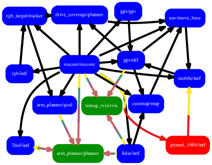
(a) Software graph

(b) Hardware graph

Figure 9: Synthesized system for the complete configuration, when operating outside, during the day, with visible targets.

In these experiments, three separate IMUs are included with different costs and connection requirements, but lacking any differentiation in performance characteristics. As a result, one option offers the lowest cost, and is utilized in every system requiring inertial measurements. This introduces a small single board computer in order to support a physical transport type unsupported by every other device ($I^{2}C$). The combination of a small single board computer and a low cost IMU was introduced to model the kind of system which might be crafted from parts readily available from a hobbyist outlet. Generally, the synthesized system treats the combination of IMU and single board computer identically to how the parts were initially introduced (e.g. as a single purpose inertial measurement module). In a small number of cases, other tasks get assigned to the single board computer, taking advantage of the available under-utilized resources. Two tasks commonly transitioned to this computer occur in Figure 9, in which the extended Kalman filter task, which utilizes the IMU measurements directly, and the RGB camera interface (and accompanying RGB camera). These cases demonstrate the power of synthesizing these systems automatically, since resources are utilized in a rigorously optimal fashion, as opposed to following local decisions.

IV-B Humanoid Disaster Response Robot Synthesis

The development of robots to address novel scenarios pushes researchers to develop more complex systems to handle real world complexities. Competitions such as the DARPA Robotics Challenge serve to focus efforts on particular scenarios and encourage pushing the state of the art in fielded systems. These systems provide an ideal case study for system synthesis - reducing time spent diagnosing errors due to missing functionality or oversubscribing resources would lead to increased productivity and safety. Hard constraints imposed by competition design and non-functional requirements derived from related efforts introduce additional need for expert knowledge to guide module capabilities. For instance, degraded communications between operator and robot imposes a hard constraint on the hardware structure, as well as guiding software development of software to respect tighter bandwidth limits. Previously developed robots can provide insight into the new design space, as well as accumulated expert knowledge. For a case study, a system synthesis problem is formulated based on the design of Team VALOR’s ESCHER and solved. As a custom humanoid, ESCHER’s design included a wide variety of custom hardware and software that had to be developed and integrated into a single, functional whole. The hardware design included 33 degrees-of-freedom with both custom (e.g. linear series elastic actuators) and off-the-shelf (e.g. MultiSense stereo vision) devices. Furthermore, the software design employs a mix of novel and open-source software covering 3 different infrastructures (ROS, LCM, and Bifrost), development shared between four different teams  [43, 34, 6] and totaling over 1.7 million source lines of code. ESCHER’s design was performed manually for the competition, providing a real world baseline to compare against.

Each design approach operates with differing levels of freedom in this comparison. Resource requirements, the organization of functionality into discrete devices or tasks, and the approach taken to meeting system requirements can evolve throughout the original development process, which cannot be captured with a ex post facto application of synthesis. Applying system synthesis on a completed design can provide insight into only the aspects of the design over which it operates - device and task interconnections, execution assignments, etc. Many of the decisions available during development cannot be considered within this framework in a single problem instance. This comparison focuses on providing some sense of how system synthesis compares to human effort in the later stages of integration and field experiments, in which both system synthesis and human experts perform equivalent tasks in design. In order to accomplish this, the final design of ESCHER is decomposed into a set of modules ($D=18$, $P=36$, $N=12$) used to generate and solve a full system synthesis problem instance.

The results of system synthesis in Figure 10 produces a system significantly different from the manually defined version. The automated design does not include two of the six computers in the original design, resulting in a more compact hardware design. In the manual design, the four onboard computers were named in reference to the deliberative paradigm of robotics: sense, think, act, and dream. A fifth computer, known as archangel, offboard the physical robot but not suffering from degraded communications, managed the network connection. Manual task assignments followed this naming convention: motion-related tasks to act, perception related tasks to sense, higher level cognitive functions to think, network management to archangel, and the remaining tasks to dream. In the synthesized system, task groupings re-occur at a coarse level on the selected computers. The differences can be summarized as placing tasks closer to necessary inputs: tasks related to mid-level perception were assigned alongside the planning tasks which utilized their outputs, while network management tasks were moved alongside tasks generating data to transmit across the bridge. Localization and networking tasks handling command and control messages were assigned alongside motion tasks with which they interacted. The high-performance IMU was assigned from an unused computer to a computer with an open RS–232 port. These results indicate that the system produces a reasonable result given its similarity to the manually designed attempt, but a lower overall cost. Synthesis uses two fewer computers, corresponding to a significantly more efficient final system. Additionally, the rearrangement of tasks results in less bandwidth usage on higher latency connections. The synthesis problem is solved in an average of $9.120s$ over five trials, fitting well within design-time operation.

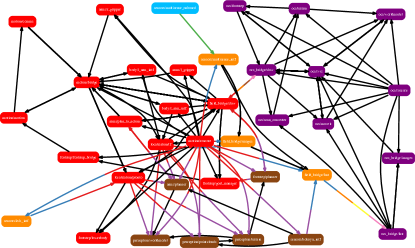
(a) Software Graph

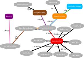
(b) Hardware Graph

Figure 10: Synthesized ESCHER system.

V Discussion & Conclusion

System synthesis captures several aspects of robot design, integrating them into a unified framework for ensuring a functional result. Introducing higher level concepts of functionality and context-awareness provide mechanisms for encoding expert knowledge about requirements at the systems engineering level, and restrictions on valid systems on the technical level, while still enforcing constraints on computing resources. These two features provide the mechanism for down-selecting core components to guide system construction. The other novel constraints introduced define a set of conditions necessary for components to operate, and that the resulting system provides a consistent solution. Integrating these constraints with the assignment and routing problem ensures that the fine grained details of constructing a viable system are handled as well. These features extend the underlying problem to provide a global solution from high level functional requirements to low level assignment concerns.

The case studies demonstrate the capabilities of this system in generating modern fielded robots. Demonstrated performance meets the design-time analysis role suggested in these experiments, automating a previously manual effort. Traditional approaches to designing computational systems for robots involves laborious trial-and-error efforts, or over-engineering the hardware aspect to ensure many viable solutions exist, without a rigorous framework for defining optimality. Automated system synthesis compares very favorably to these approaches, ensuring an optimal solution while providing a framework for quantifying several aspects of the design.

V-A Practical Considerations

As a design-time tool, it is worth remarking on several important observations from these experiments. In constructing the presented experiments, significant effort was expended in formulating correct, re-usable, and consistent specifications. These issues generally derive from increased specificity in system details, differing aims in development tools, and defining functionality and context in a re-usable fashion.

The need for precise quantitative values to define system synthesis problems drives one of the biggest changes in these experiments. Generally, systems focus on functionality first, and addressing finer grained details such as bandwidth utilization or computational constraints are addressed later. System synthesis operates holistically, requiring quantified values at every scale in order to produce a complete problem. In practice, many low level details (e.g. CPU or memory utilization) are left under- or un- quantified, with hardware components selected to provide significant overhead in these resources. Accurately estimating parameters for non-functional requirements, or connectivity between tasks requires careful parsing through layers of abstraction and indirection. Initially using pessimistic estimates costs relatively little effort compared to attempting to quantify these details earlier on. This approach should be mirrored in system synthesis, with resource parameters estimated as worst-case estimates, producing a similar preference towards over-provisioning. With automatic system synthesis, tools which can help refine these estimates as a design evolves are useful for understanding the overall design space. Small-scale parameter changes can ripple throughout a design, and additional support for mapping higher level decisions down to quantifiable results would be beneficial. The inclusion of traditionally less heavily scrutinized parameters enables more rigorous system synthesis, but care must be taken in applying well established design practices to these aspects of system analysis.

Finally, the definition of semantic parameters across components require careful consideration and development. Current systems rarely provide explicit definitions of the semantic content of algorithm inputs and outputs in a reusable fashion. The development and presentation of novel components focuses on the demonstration of success for a particular application or challenge. Defining the operational envelope for a component requires analyzing and understanding failure as well, which not only increases effort, but introduces analysis to extract root causes related to technically relevant parameters. Furthermore, some of these parameters may be relevant only to a subset of developers. For instance, a task input may have a semantic requirement of representing a goal state for planning, which represents the universal version of that requirement. A system which may optionally include multiple sources of that particular goal state (e.g. an autonomous system and an operator) which requires expanding the semantic requirement to represent both the source and the content of the data as aspects of the semantic requirement. These problems reach towards the need to better understand and communicate how re-usable elements can be shared, a more general problem beyond the scope of this work.

V-B Future Work

Posing system synthesis as an integer program results in solving for the global optimum, requiring more computational effort to find the solution. Switching to approaches capable of quickly finding approximately optimal solutions raises the possibility of extending the range of problems which can solve in an online scenario. Extending this approach to address hardware fault recovery, dynamic operational contexts or mission requirements offers the ability to be more resilient in the face of failures. Dynamically altering the hardware and software as requirements and context change can offer greater adaptability, allowing components developed to address specialized scenarios to be used when necessary. Generally, online execution of system synthesis can enable reasoning about interactions between a system’s structure and the environment, potentially enabling a wide variety of new capabilities.

Another avenue of work introduces reasoning about the physical relationships between elements under consideration. Hardware connections currently serve to transfer data between devices; connections can also transfer power, add payload mass, or enforce mechanical relationships between elements. Generalizing hardware connections can allow reasoning about additional hardware constraints such as power and mass budgets. Additionally, consideration of mechanical relationships between elements can improve expressiveness in synthesizing multi-robot systems, as well as enabling more expressive constraints on mechanical systems (e.g. ensuring an IMU is rigidly mounted on each robot, or selecting mobility elements based on environment).

Introducing a more robust model for functionality could improve the complexity of design problems posed in this framework. Currently, functionality is modeled as linearly independent parameters, which does not reflect some functional trade-offs in design. Interactions between functional elements can include synergistic effects (e.g. better localization improving accuracy for perception), adversarial relationships (e.g. assigning more roles to a single robot reducing the time devoted to each role), or non-linear scaling (e.g. running two localization estimators may not linearly improve the accuracy of localization). Reworking the model for how functional elements contribute to the overall system opens the door to a wider variety of design considerations.

Escher

References

- [1] Ioan A. Sucan and Sachin Chitta “MoveIt!”, 2017 URL: http://moveit.ros.org
- [2] Armin Hornung et al. “OctoMap: An Efficient Probabilistic 3D Mapping Framework Based on Octrees” In Autonomous Robots, 2013 DOI: 10.1007/s10514-012-9321-0
- [3] Jakob Engel, Thomas Schöps and Daniel Cremers “LSD-SLAM: Large-Scale Direct Monocular SLAM” In Computer Vision – ECCV 2014: 13th European Conference, Zurich, Switzerland, September 6-12, 2014, Proceedings, Part II, 2014, pp. 834–849 DOI: 10.1007/978-3-319-10605-2{\_}54
- [4] Armin Hornung, Andrew Dornbush, Maxim Likhachev and Maren Bennewitz “Anytime search-based footstep planning with suboptimality bounds” In 2012 12th IEEE-RAS International Conference on Humanoid Robots (Humanoids 2012), 2012, pp. 674–679 IEEE DOI: 10.1109/HUMANOIDS.2012.6651592
- [5] Morgan Quigley et al. “ROS: an open-source Robot Operating System” In ICRA 3, 2009, pp. 5 DOI: http://www.willowgarage.com/papers/ros-open-source-robot-operating-system
- [6] Coleman Knabe et al. “Team VALOR’s ESCHER: A Novel Electromechanical Biped for the DARPA Robotics Challenge” In Journal of Field Robotics, 2017 DOI: 10.1002/rob.21697
- [7] Mathew DeDonato et al. “Team WPI-CMU: Achieving Reliable Humanoid Behavior in the DARPA Robotics Challenge” In Journal of Field Robotics, 2017 DOI: 10.1002/rob.21685
- [8] “Rock, the Robot Construction Kit”, 2017 URL: http://www.rock-robotics.org
- [9] Paul Fitzpatrick, Giorgio Metta and Lorenzo Natale “Towards Long-lived Robot Genes” In Robotics and Autonomous Systems 56.1 Amsterdam, The Netherlands, The Netherlands: North-Holland Publishing Co., 2008, pp. 29–45 DOI: 10.1016/j.robot.2007.09.014
- [10] David Stewart, Richard Volpe and Pradeep Khosla “Design of Dynamically Reconfigurable Real-Time Software Using Port-Based Objects” In IEEE Transactions on Software Engineering 23.12, 1997
- [11] Yanzhe Cui, Richard M Voyles, Joshua T Lane and Mohammad H Mahoor “ReFrESH: A Self-Adaptation Framework to Support Fault Tolerance in Field Mobile Robots”, 2014, pp. 1576–1582
- [12] Yanzhe Cui, Joshua T Lane and Richard M Voyles “Real-Time Software Module Design Framework for Building Self-Adaptive Robotic Systems”, 2015, pp. 2597–2602
- [13] David Doose, Christophe Grand and Charles Lesire “MAUVE Runtime: A Component-Based Middleware to Reconfigure Software Architectures in Real-Time” In 2017 First IEEE International Conference on Robotic Computing (IRC), 2017, pp. 208–211 DOI: 10.1109/IRC.2017.47
- [14] David W. Pentico “Assignment problems: A golden anniversary survey” In European Journal of Operational Research 176.2, 2007, pp. 774–793 DOI: 10.1016/j.ejor.2005.09.014
- [15] Eliane Maria Loiola et al. “A survey for the quadratic assignment problem” In European Journal of Operational Research 176.2, 2007, pp. 657–690 DOI: 10.1016/j.ejor.2005.09.032
- [16] G.. Ross and R.. Soland “A branch and bound algorithm for the generalized assignment problem” In Mathematical Programming 8.1, 1975, pp. 91–103 DOI: 10.1007/BF01580430
- [17] J.E. Beck and D.P. Siewiorek “Modeling Multicomputer Task Allocation as a Vector Packing Problem” In Proceedings of the 9th International Symposium on System Synthesis (ISSS 96), 1996, pp. 115–120 DOI: 10.1109/ISSS.1996.565892
- [18] S. Even, A. Itai and A. Shamir “On the complexity of time table and multi-commodity flow problems” In 16th Annual Symposium on Foundations of Computer Science (sfcs 1975), 1975, pp. 184–193 DOI: 10.1109/SFCS.1975.21
- [19] T.. ter Braak, G… Smit and P… Hölzenspies “Dynamic Resource Allocation Problems”, 2016 URL: http://eprints.eemcs.utwente.nl/26878/
- [20] Han-Lim Choi, L. Brunet and J.P. How “Consensus-Based Decentralized Auctions for Robust Task Allocation” In Robotics, IEEE Transactions on 25.4, 2009, pp. 912–926 DOI: 10.1109/TRO.2009.2022423
- [21] P.B. Sujit and R. Beard “Distributed Sequential Auctions for Multiple UAV Task Allocation” In American Control Conference, 2007. ACC ’07, 2007, pp. 3955–3960 DOI: 10.1109/ACC.2007.4282558
- [22] Xiaoming Zheng, S. Koenig and C. Tovey “Improving Sequential Single-Item Auctions” In Intelligent Robots and Systems, 2006 IEEE/RSJ International Conference on, 2006, pp. 2238–2244 DOI: 10.1109/IROS.2006.282567
- [23] M.G. Lagoudakis et al. “Simple auctions with performance guarantees for multi-robot task allocation” In Intelligent Robots and Systems, 2004. (IROS 2004). Proceedings. 2004 IEEE/RSJ International Conference on 1, 2004, pp. 698–705 vol.1
- [24] D P Bertsekas “The auction algorithm: A distributed relaxation method for the assignment problem” In Annals of Operations Research 14.1, 1988, pp. 105–123 DOI: 10.1007/BF02186476
- [25] Michael M Zavlanos, Leonid Spesivtsev and George J Pappas “A distributed auction algorithm for the assignment problem” In IEEE Conference on Decision and Control, 2008, pp. 1212–1217 DOI: 10.1109/CDC.2008.4739098
- [26] Lingzhi Luo, N. Chakraborty and K. Sycara “Provably-Good Distributed Algorithm for Constrained Multi-Robot Task Assignment for Grouped Tasks” In Robotics, IEEE Transactions on 31.1, 2015, pp. 19–30 DOI: 10.1109/TRO.2014.2370831
- [27] Ryan K. Williams, Andrea Gasparri and Giovanni Ulivi “Decentralized Matroid Optimization for Topology Constraints in Multi-Robot Allocation Problems” In Robotics and Automation (ICRA), 2017 IEEE International Conference on, 2017
- [28] Robert Michael Zlot and Anthony Stentz “Market-based Multirobot Coordination for Complex Tasks” In International Journal of Robotics Research, Special Issue on the 4th International Conference on Field and Service Robotics 25.1, 2006, pp. 73–101
- [29] Brian P. Gerkey and Maja J. Mataric “A Formal Analysis and Taxonomy of Task Allocation in Multi-Robot Systems” In The International Journal of Robotics Research 23.9, 2004, pp. 939–954 DOI: 10.1177/0278364904045564
- [30] G. Korsah, Anthony Stentz and M. Dias “A comprehensive taxonomy for multi-robot task allocation” In The International Journal of Robotics Research 32.12, 2013, pp. 1495–1512 DOI: 10.1177/0278364913496484
- [31] A. Censi “A Mathematical Theory of Co-Design” In ArXiv e-prints, 2015 arXiv:1512.08055 [cs.LO]
- [32] Ruta Desai, Yuan Ye and Stelian Coros “Computational Abstractions for Interactive Design of Robotic Devices” In IEEE International Conference on Robotics and Automation (ICRA), 2017
- [33] Sehoon Ha et al. “Joint Optimization of Robot Design and Motion Parameters using the Implicit Function Theorem” In Robotics: Science and Systems, 2017
- [34] Maurice F Fallon, Matthew Antone, Nicholas Roy and Seth Teller “Drift-free humanoid state estimation fusing kinematic, inertial and LIDAR sensing” In 2014 IEEE-RAS International Conference on Humanoid Robots IEEE, 2014, pp. 112–119 DOI: 10.1109/HUMANOIDS.2014.7041346
- [35] Hugh Durrant-Whyte and Tim Bailey “Simultaneous Localization and Mapping: Part I” In IEEE Robotics Automation Magazine 13.2, 2006, pp. 99–110 DOI: 10.1109/MRA.2006.1638022
- [36] Shahram Izadi et al. “KinectFusion: Real-time 3D Reconstruction and Interaction Using a Moving Depth Camera” In Proceedings of the 24th Annual ACM symposium on User Interface Software and Technology, UIST ’11 Santa Barbara, California, USA: ACM, 2011, pp. 559–568 DOI: 10.1145/2047196.2047270
- [37] Alonzo Kelly “Mobile Robotics: Mathematics, Models, and Methods” Cambridge University Press, 2013
- [38] Max Reichardt, Tobias Föhst and Karsten Berns “Introducing FINROC: A Convenient Real-Time Framework for Robotics Based on a Systematic Design Approach”, 2012, pp. 1–8 URL: https://agrosy.informatik.uni-kl.de/fileadmin/Literatur/Reichardt12.pdf
- [39] Matthew Mcnaughton et al. “Software Infrastructure for an Autonomous Ground Vehicle” In Journal of Aerospace Computing Information and Communication 5.12, 2008, pp. 491–505 DOI: 10.2514/1.39487
- [40] Kevin J Sullivan, William G Griswold, Yuanfang Cai and Ben Hallen “The structure and value of modularity in software design” In ACM SIGSOFT Software Engineering Notes 26.5, 2001, pp. 99 DOI: 10.1145/503271.503224
- [41] T.. Braak “Using guided local search for adaptive resource reservation in large-scale embedded systems” In 2014 Design, Automation Test in Europe Conference Exhibition (DATE), 2014, pp. 1–4 DOI: 10.7873/DATE.2014.171
- [42] Gurobi Optimization Inc. “Gurobi Optimizer Reference Manual”, 2016 URL: http://www.gurobi.com
- [43] Alberto Romay et al. “Collaborative Autonomy between High-level Behaviors and Human Operators for Remote Manipulation Tasks using Different Humanoid Robots” In Journal of Field Robotics 34.2, 2017, pp. 333–358 DOI: 10.1002/rob.21671