Existence theory for magma equations in dimension two and higher

Abstract.

We examine a degenerate, dispersive, nonlinear wave equation related to the evolution of partially molten rock in dimensions two and higher. This simplified model, for a scalar field capturing the melt fraction by volume, has been studied by direct numerical simulation where it has been observed to develop stable solitary waves. In this work, we prove local in time well-posedness results for the time dependent equation, on both the whole space and the torus, for dimensions two and higher. We also prove the existence of the solitary wave solutions in dimensions two and higher.

1. Introduction

Consistent systems of partial differential equations governing the flow of partially molten rock in the Earth’s interior began appearing in the 1980s in [11, 15]. These models captured the essential features of the mechanics of partial melts. Important features include: there are at least two phases (the molten rock, which behaves as a true fluid, and a residual porous matrix of rock); the molten rock migrates via porous flow through the residual matrix; on the geologic time scale of tens or hundreds of thousands of years, the matrix deforms viscously; and inertia can be neglected in both phases due to the highly viscous nature of the problem.

These models typically take the form:

(1.1a) $$\partial_{t}(\rho_{\rm melt}\phi)+\nabla\cdot(\rho_{\rm melt}\phi{\bf v}_{\rm melt})=\hphantom{-}\text{Melting/Freezing},$$

(1.1b) $$\partial_{t}(\rho_{\rm matrix}(1-\phi))+\nabla\cdot(\rho_{\rm matrix}(1-\phi){\bf v}_{\rm matrix})=-\text{Melting/Freezing},$$

(1.1c) $$\phi({\bf v}_{\rm melt}-{\bf v}_{\rm matrix})=-\tfrac{k_{\rm matrix}}{\mu_{\rm melt}}(\nabla p-\rho_{\rm melt}g{\bf z}),$$

(1.1d) $$\begin{split}0=\bar{\rho}g{\bf z}-\nabla p&+\nabla\cdot[2(1-\phi)\mu_{\rm matrix}\dot{e}_{\rm matrix}]\\ &+\nabla[(1-\phi)(\zeta_{\rm matrix}-\tfrac{2}{3}\mu_{\rm matrix})\nabla\cdot{\bf v}_{\rm matrix}].\end{split}$$

In the above expressions, $\rho_{\rm melt}$ and $\rho_{\rm matrix}$ are the densities of the melt and matrix phases, while ${\bf v}_{\rm melt}$ and ${\bf v}_{\rm matrix}$ are the velocities. The porosity, $\phi$, is the volume fraction of melt, and $p$ is the pressure. Thus, (1.1a) and (1.1b) merely state conservation of mass between the two phases; additional thermodynamic information must be provided to derive phase changes.

The reader may recognize (1.1c) as Darcy’s Law, with $k_{\rm matrix}$ the permeability of the matrix, $\mu_{\rm melt}$ the shear viscosity of the melt, $p$ the (joint) fluid pressure, and $g{\bf z}$ the buoyancy force. Lastly, (1.1d) reflects the force balance in the matrix, with $\mu_{\rm matrix}$ its shear viscosity, $\dot{e}_{\rm matrix}$ the strain rate, and $\zeta_{\rm matrix}$ the bulk viscosity. Constitutive relations must be introduced for the viscosities and the permeability, as they typically depend on the porosity.

Models like this have been revisited, rederived, and extended in a variety of ways, with novel predictions for large scale Earth dynamics; see, for example, [3, 4, 13, 18, 19, 24, 25, 9, 27, 26, 28, 29, 8].

1.1. The Scalar Magma Equation

Under a series of approximations, one can obtain the reduced model,

(1.2) $$\phi_{t}+\partial_{x_{d}}\left(\phi^{n}\right)-\nabla\cdot\left(\phi^{n}\nabla\phi_{t}\right)=0.$$

Here, $\phi$ is the rescaled porosity, with units of $\phi_{0}<1$, a characteristic value.

Following the derivation of [23, 21], (1.2) can be obtained from (1.1) as follows. First, we neglect phase changes in (1.1a) and (1.1b) and assume constant density of each phase. After dividing out by the density and adding the two equations,

(1.3) $$\nabla\cdot[\phi{\bf v}_{\rm melt}+(1-\phi){\bf v}_{\rm matrix}]=0.$$

The divergence of (1.1c) is then taken, and (1.3) is used to eliminate ${\bf v}_{\rm melt}$,

(1.4) $$\nabla\cdot{\bf v}_{\rm matrix}=\nabla\cdot\left[\tfrac{k_{\rm matrix}}{\mu_{\rm melt}}(\nabla p-\rho_{\rm melt}g{\bf z})\right].$$

If we now assume that the shear viscosities are constants, then, after applying a vector identity,

$$\begin{split}-\mu_{\rm matrix}\nabla\times\nabla\times{\bf v}_{\rm matrix}&+\nabla\left[((1-\phi)\zeta_{\rm matrix}+\tfrac{4}{3}\mu_{\rm matrix})\nabla\cdot{\bf v}_{\rm matrix}\right]\\ &\quad-(1-\phi)\Delta\rho{\bf z}=\nabla p-\rho_{\rm melt}g{\bf z}.\end{split}$$

Letting $\mathcal{C}=\nabla\cdot{\bf v}_{\rm matrix}$ be the compaction rate, and assuming there are no large scale shear motions,

$$\nabla\left[((1-\phi)\zeta_{\rm matrix}+\tfrac{4}{3}\mu_{\rm matrix})\mathcal{C}\right]-(1-\phi)\Delta\rho{\bf z}=\nabla p-\rho_{\rm melt}g{\bf z}.$$

Multiplying this equation by $k_{\rm matrix}/\mu_{\rm melt}$ and taking the divergence, $\nabla p-\rho_{\rm melt}g{\bf z}$ can be eliminated with (1.4) to obtain,

(1.5) $$\mathcal{C}-\nabla\cdot\left\{\tfrac{k_{\rm matrix}}{\mu_{\rm melt}}\nabla\left[((1-\phi)\zeta_{\rm matrix}+\tfrac{4}{3}\mu_{\rm matrix})\mathcal{C}\right]\right\}=-\nabla\cdot\left[\tfrac{k_{\rm matrix}}{\mu_{\rm melt}}(1-\phi)\Delta\rho g{\bf z}\right].$$

If we now make the commonly used approximations that $k_{\rm matrix}=k_{0}\phi^{n}$ and $\zeta_{\rm matrix}$ is constant, then, after nondimensionalization, (1.5) and (1.1b) become

$$\partial_{t^{\prime}}\phi^{\prime}=-\phi_{0}\nabla^{\prime}\phi^{\prime}\cdot{\bf v}^{\prime}_{\rm matrix}+(1-\phi_{0}\phi^{\prime})\mathcal{C}^{\prime},$$

$$\begin{split}&\mathcal{C}^{\prime}-\nabla^{\prime}\cdot\left\{(\phi^{\prime})^{n}\nabla^{\prime}\left[\left(\frac{(1-\phi_{0}\phi^{\prime})\zeta_{\rm matrix}+\tfrac{4}{3}\mu_{\rm matrix})}{(1-\phi_{0})\zeta_{\rm matrix}+\tfrac{4}{3}\mu_{\rm matrix})}\right)\mathcal{C}\right]\right\}\\ &\hskip 180.67499pt=-\nabla^{\prime}\cdot\left[\frac{1-\phi_{0}\phi^{\prime}}{1-\phi_{0}}(\phi^{\prime})^{n}{\bf z}\right].\end{split}$$

Finally, if the characteristic porosity is small, i.e., $0<\phi_{0}\ll 1$, these two equations become

$$\partial_{t^{\prime}}\phi^{\prime}=\mathcal{C}^{\prime},$$

$$\mathcal{C}^{\prime}-\nabla^{\prime}\cdot\left\{(\phi^{\prime})^{n}\nabla^{\prime}\mathcal{C}^{\prime}\right\}=-\nabla^{\prime}\cdot\left((\phi^{\prime})^{n}{\bf z}\right).$$

Substituting the first equation into the second, and dropping the primes, we recover (1.2).

1.2. Properties of the Scalar Equation

In Equation (1.2), the temporal variable satisfies $t>0$, and the spatial variable satisfies $\mathbf{x}\in{\bf{T}}^{d}$ or $\mathbf{x}\in{\bf{R}}^{d}$. The dependent variable $\phi=\phi(\mathbf{x},t)\in{\bf{R}}$ is the porosity of the media, corresponding to volume fraction that is melt. The nonlinearity, $\phi^{n}$, reflects the permeability of the solid rock, with typical physical values of $n\in[2,3]$. Equation (1.2) is sometimes called “the magma equation,” a terminology we adopt here, and this reduced model is the focus of this work.

Some of the key features of (1.2) are that it is dispersive, degenerate, and nonlocal. To see the dispersive aspect, if we formally linearize as $\phi=\phi_{0}+\epsilon e^{i(\mathbf{k}\cdot\mathbf{x}-\omega t)}$ with $\phi_{0}>0$, one obtains the dispersion relation

$$\omega(\mathbf{k})=\frac{n\phi_{0}^{n-1}k_{d}}{1+\phi_{0}^{n}|\mathbf{k}|^{2}}.$$

The degeneracy can be seen in the highest derivative term in the event that $\phi\to 0$. The nonlocality can be seen by rewriting (1.2) as

(1.6a) $$\phi_{t} =\mathcal{C},$$

(1.6b) $$[I-\nabla\cdot(\phi^{n}\nabla\bullet)]\mathcal{C} =-\partial_{x_{d}}(\phi^{n}).$$

Suppose that $\phi$ is given such that $\phi$ is non-negative and sufficiently smooth. Then subject to boundary conditions, (1.6b) is elliptic with respect to $\mathcal{C}$. Having solved the elliptic equation for $\mathcal{C}$, (1.6a) gives us the time derivative of $\phi$. This matter of maintaining ellipticity of (1.6b) is at the heart of analyzing (1.2).

Numerical simulations of (1.2) have been conducted in dimensions $d=1,2,3$, usually with the boundary condition that $\phi\to 1$ as $|\mathbf{x}|\to\infty$. This is often approximated on a large periodic domain. In addition, initial data tends to break up into rank-ordered traveling solitary waves. These waves propagate in the preferred direction $x_{d}$ and are radially symmetric in a comoving frame, and have been observed to be stable. While they are not expected to be integrable, the solitary waves have been observed to have elastic-like collisions. The solitary waves can be obtained with the ansatz,

(1.7) $$\phi(\mathbf{x},t)=\bar{Q}(\bar{r}(\mathbf{x},t)),\quad\bar{r}^{2}(\mathbf{x},t)=\sum_{j=1}^{d-1}x_{j}^{2}+(x_{d}-\bar{c}t)^{2}.$$

For examples, see [16, 15, 14, 2, 1, 30].

While these numerical studies have been fruitful for understanding the dynamics of the equation, and for gaining insight into the larger system of equations from which it has been derived, relatively little has been done to analyze (1.2). In [17], the authors established local and global in time well-posedness results in $d=1$ by fixed point iteration methods in Sobolev spaces. In [12], the authors proved the existence of traveling waves in $d=1$ with wave speed $c>n>1$, asymptotically converging to unity as $x\to\pm\infty$. This is accomplished in $d=1$ by obtaining a first integral. Some additional regularity properties of the solutions were obtained in [20], and their stability was studied in that work, along with [22]. However, to the best of the authors’ knowledge, no mathematically rigorous results have been obtained for $d\geq 2$.

1.3. Main Results

In this work, we aim to establish local-in-time well-posedness results for (1.2) in dimensions $d\in{\bf{Z}}$, $d\geq 2$. We also establish the existence of traveling solitary waves in dimensions $d\in{\bf{N}}$. These results are:

Theorem 1.1.

Let $s\in{\bf{N}}$ such that $s>d/2+\lfloor d/2\rfloor+2$ and let

$$U\equiv\left\{f-1\in H^{s}({\bf{R}}^{d}):\|1/f\|_{L^{\infty}({\bf{R}}^{d})}<\infty\text{ and }f>0\right\},$$

and assume $\phi_{0}\in U$.

There exists $T_{\alpha}<0<T_{\omega}$ and $\phi\in C^{1}((T_{\alpha},T_{\omega});U)$ with $\phi(0)=\phi_{0}$ such that $\phi$ satisfies (1.2) for all $t\in(T_{\alpha},T_{\omega})$.

$T_{\omega}$ (respectivley $T_{\alpha}$) is maximal in the following sense that we have the dichotomy:

1. $T_{\omega}=+\infty$ (respectivley $T_{\alpha}=-\infty$), or

2. $\lim_{t\to T_{\omega}^{-}}\left(\|\phi(t)-1\|_{H^{s}({\bf{R}}^{d})}+\|1/\phi(t)\|_{L^{\infty}({\bf{R}}^{d})}\right)=+\infty$
   (respectivley $\displaystyle\lim_{t\to T_{\alpha}^{+}}\left(\|\phi(t)-1\|_{H^{s}({\bf{R}}^{d})}+\|1/\phi(t)\|_{L^{\infty}({\bf{R}}^{d})}\right)=+\infty$ ).

The essential ingredient in this theorem is that if the data is continuous and bounded from below away from zero, it remains so for the time of existence. While this result is stated in terms of ${\bf{R}}^{d}$, an analogous result will be shown to hold in ${\bf{T}}^{d}$, where many simulations are performed.

We also prove an existence theorem for radially symmetric traveling solitary waves satisfying (1.7). These solutions are unimodal and converge at spatial infinity to a constant state. Specifically, we show:

Theorem 1.2.

For each $d\in{\bf{N}}$, $n\in[2,3]$, and $c\in[1.55,n)$, there exists a smooth function $Q:{\bf{R}}_{\geq 0}\to{\bf{R}}$ with the following properties:

1. $Q(0)=1$, $Q_{r}(0)=0$, and $Q_{rr}(0)<0$. Here, $Q_{r}$ and $Q_{rr}$ denote the first and second derivatives of $Q(r)$, respectively.

2. $Q_{r}(r)<0$ for all $r>0$.

3. $\lim_{r\to\infty}Q(r)$ exists, and $0<\lim_{r\to\infty}Q(r)<1$.

4. For every $\bar{q}_{0}>0$, putting $\phi(\mathbf{x},t)=\bar{Q}\left(|\mathbf{x}-\bar{c}t{\bf e}_{d}|\right)=\bar{q}_{0}Q\big{(}\bar{q}_{0}^{-\frac{n}{2}}|\mathbf{x}-\bar{c}t{\bf e}_{d}|\big{)}$ solves (1.2) with $\bar{c}=\bar{q}_{0}^{n-1}c$.

1.4. Outline

In Section 2, we prove our local-in-time well-posedness results. In Section 3, we establish the existence of the solitary waves. We conclude with some remarks in Section 4.

2. Well-posedness

2.1. Elliptic Estimates

We begin by establishing some elliptic estimates for the problem on ${\bf{T}}^{d}$ and ${\bf{R}}^{d}$. Let

$$L_{a}u:=u-\nabla\cdot(a\nabla u).$$

Throughout, we will assume that $a>0$, either because it is a continuous function, or because it can be replaced a continuous version which is positive. Throughout, we will use $\Pi$ to denote a polynomial in its arguments, assumed to have positive coefficients.

2.1.1. Problem on ${\bf{T}}^{d}$

First, we recall a standard elliptic regularity result, which can be found in, for instance, [5, 6].

Theorem 2.1.

Suppose that $m\in{\bf{N}}$, $a\in C^{m+1}({\bf{T}}^{d})$, $a>0$, $1/a\in L^{\infty}({\bf{T}}^{d})$, and $g\in H^{m}({\bf{T}}^{d})$. There exists a unique function $u\in H^{m+2}({\bf{T}}^{d})$ such that $L_{a}u=g$. Moreover,

(2.1) $$\|u\|_{H^{m+2}({\bf{T}}^{d})}\leq\Pi\left(\|a\|_{C^{m+1}({\bf{T}}^{d})},\|1/a\|_{L^{\infty}({\bf{T}}^{d})}\right)\|g\|_{H^{m}({\bf{T}}^{d})}.$$

$\Pi$ depends only on $m$ and $d$.

Also recall the Sobolev embedding theorem:

Theorem 2.2.

Let $s>d/2$ and $s\in{\bf{N}}$. There exists $C=C(s,d)>0$ such that for all $u\in H^{s}({\bf{T}}^{d})$ one has

$$\|u\|_{C^{s-\lfloor d/2\rfloor-1}({\bf{T}}^{d})}\leq C\|u\|_{H^{s}({\bf{T}}^{d})}.$$

This has the following consequence:

Corollary 2.3.

Suppose that $s>d$ and $s\in{\bf{N}}$. If $f\in H^{s}({\bf{T}}^{d})$ and $1/f\in L^{\infty}({\bf{T}}^{d})$, then $1/f\in H^{s}({\bf{T}}^{d})$ and

$$\left\|{1/f}\right\|_{H^{s}({\bf{T}}^{d})}\leq\Pi\left(\|f\|_{H^{s}({\bf{T}}^{d})},\left\|{1/f}\right\|_{L^{\infty}({\bf{T}}^{d})}\right).$$

$\Pi$ depends only on $s$ and $d$.

Proof.

This follows from the previous theorem and the chain rule; upon differentiating $1/f$ as many as $s$ times, one arrives at a sum of a number of terms which involve in the numerator products of up to $s$ derivatives of $f,$ with factors of $f$ in the denominator. The factors of $f$ in the denominator are bounded in $L^{\infty}$ since we have assumed $1/f\in L^{\infty}.$ The products in the numerator are bounded in $L^{2}$ since in any such product, only one factor may have more than $s/2$ derivatives, and thus only one factor might fail to be in $L^{\infty};$ this factor, then, may be estimated in $L^{2}$ while the remaining factors may be estimated using Sobolev embedding. ∎

We next extend (2.1) to obtain an elliptic regularity result essential to this work,

Proposition 2.4.

Let $s>{d/2}+\lfloor d/2\rfloor+1$ and $s\in{\bf{N}}$. Suppose that $a\in H^{s}({\bf{T}}^{d})$, $a>0$, $1/a\in L^{\infty}({\bf{T}}^{d})$ and $g\in H^{s-1}({\bf{T}}^{d})$. Then there exists a unique function $u\in H^{s+1}({\bf{T}}^{d})$ such that $L_{a}u=g$. Moreover,

(2.2) $$\|u\|_{H^{s+1}({\bf{T}}^{d})}\leq\Pi\left(\|a\|_{H^{s}({\bf{T}}^{d})},\|1/a\|_{L^{\infty}({\bf{T}}^{d})}\right)\|g\|_{H^{s-1}({\bf{T}}^{d})}.$$

$\Pi$ depends only on $s$ and $d$.

Proof.

First, by Theorem 2.1 we have $a\in C^{s-\lfloor d/2\rfloor-1}({\bf{T}}^{d})$. Let $m:={s-\lfloor d/2\rfloor-2}$. The conditions on $s$ guarantee that $0\leq m\leq s-1$. We therefore find $a\in C^{m+1}({\bf{T}}^{d})$ and $g\in H^{m}({\bf{T}}^{d})$. Theorem 2.1 implies that there exists a unique $u\in H^{m+2}({\bf{T}}^{d})$ for which $L_{a}u=g$ and the estimate in that theorem holds,

(2.3) $$\|u\|_{H^{m+2}}\leq\Pi(\|a\|_{C^{m+1}},\|1/a\|_{L^{\infty}})\|g\|_{H^{m}}\leq\Pi(\|a\|_{H^{s}},\|1/a\|_{L^{\infty}})\|g\|_{H^{s-1}}.$$

Since $u\in H^{2}$, we have a strong solution in the sense that we can rewrite $L_{a}u=g$ as

$$-\Delta u=-\frac{1}{a}u+\frac{1}{a}\nabla a\cdot\nabla u+\frac{1}{a}g,$$

with equality holding in $L^{2}$. Adding $u$ to both sides gives

(2.4) $$u-\Delta u=\left(1-\frac{1}{a}\right)u+\frac{1}{a}\nabla a\cdot\nabla u+\frac{1}{a}g.$$

Next, we observe that if $u\in H^{k+1}$, for any $k>d/2$, then the right-hand side of (2.4) is in $H^{k\wedge(s-1)}$ (here, we use the notation $a\wedge b=\min\{a,b\}$); this follows from our constraints on $s$ and the assumed regularity of $a$ and $g$. Since $u\in H^{m+2},$ we may take $k$ to satisfy $k=m+1>d/2.$ By virtue of elliptic regularity, if $u\in H^{k+1}$ and if the right-hand side of (2.4) is in $H^{k\wedge(s-1)}$, then in fact $u\in H^{\left(k\wedge(s-1)\right)+2}$. If $k\wedge(s-1)=s-1,$ then this implies $u\in H^{s+1}.$ Otherwise, we may repeat this process. This bootstrap process can be continued until we conclude $u\in H^{s}$, at which point the right hand side is limited to being in $H^{s-1},$ because of the regularity of $a$ and $g.$ A final application of elliptic regularity gives $u\in H^{s+1}$.

To obtain the bound on $\|u\|_{H^{s+1}}$, we take the $H^{k}$ norm of both sides of (2.4), to get

(2.5) $$\|u\|_{H^{k+2}({\bf{T}}^{d})}\leq\left\|\left(\frac{1}{a}-1\right)u\right\|_{H^{k}({\bf{T}}^{d})}+\left\|\frac{1}{a}\nabla a\cdot\nabla u\right\|_{H^{k}({\bf{T}}^{d})}+\left\|\frac{1}{a}g\right\|_{H^{k}({\bf{T}}^{d})}.$$

For $k\in(d/2,s-1]\cap{\bf{N}}$,

$$\begin{split}\|u\|_{H^{k+2}}&\leq C\left(1+\left\|1/a\right\|_{H^{k}}+\left\|1/a\right\|_{H^{k}}\|a\|_{H^{k+1}}\right)\left\|u\right\|_{H^{k+1}}+\left\|1/a\right\|_{H^{k}}\left\|g\right\|_{H^{k}}\\ &\leq\underbrace{C\left(1+\left\|1/a\right\|_{H^{s}}+\left\|1/a\right\|_{H^{s}}\|a\|_{H^{s}}\right)}_{\equiv C_{a}}\|u\|_{H^{k+1}}+\underbrace{\left\|1/a\right\|_{H^{s}}\left\|g\right\|_{H^{s-1}}}_{\equiv B_{a,g}}.\end{split}$$

Note that in this estimate we have used Corollary 2.3, since $s>d$ and thus $1/a\in H^{s}.$ By induction and our estimate (2.3) on the $H^{m+2}$ norms, we have:

$$\begin{split}\|u\|_{H^{s+1}}&\leq C_{a}^{\lfloor d/2\rfloor}\|u\|_{H^{m+2}}+B_{a,g}\sum_{j=0}^{\lfloor d/2\rfloor}C_{a}^{j}\\ &\leq C_{a}^{\lfloor d/2\rfloor}\Pi(\|a\|_{H^{s}},\|1/a\|_{L^{\infty}})\|g\|_{H^{s-1}}+B_{a,g}\sum_{j=0}^{\lfloor d/2\rfloor}C_{a}^{j}.\end{split}$$

The conclusion, (2.2), now follows by again applying Corollary 2.3. ∎

Corollary 2.5.

Let $s>{d/2}+\lfloor d/2\rfloor+1$ and $s\in{\bf{N}}$. Suppose that $a,b\in H^{s}({\bf{T}}^{d})$, $1/a,1/b\in L^{\infty}({\bf{T}}^{d})$ and $g\in H^{s-1}({\bf{T}}^{d})$. Let $u\in H^{s+1}({\bf{T}}^{d})$ and $v\in H^{s+1}({\bf{T}}^{d})$ be the functions whose existence is implied by Proposition 2.4 such that $L_{a}u=L_{b}v=g$. Then

(2.6) $$\|u-v\|_{H^{s+1}}\leq\Pi\left(\|a\|_{H^{s}},\|1/a\|_{L^{\infty}},\|b\|_{H^{s}},\|1/b\|_{L^{\infty}}\right)\|g\|_{H^{s-1}}\|a-b\|_{H^{s}}.$$

$\Pi$ depends only on $s$ and $d$.

Proof.

Let $\eta:=u-v$. A straightforward calculation shows that $L_{b}\eta=\nabla\cdot\left((a-b)\nabla u\right)=:\tilde{g}$. We know that $u\in H^{s+1}({\bf{T}}^{d})$ and $a,b\in H^{s}({\bf{T}}^{d})$ and thus $\tilde{g}\in H^{s-1}({\bf{T}}^{d})$. In particular, since the condition on $s$ implies that $H^{s}({\bf{T}}^{d})$ is an algebra, we have:

$$\|\tilde{g}\|_{H^{s-1}}=\|\nabla\cdot\left((a-b)\nabla u\right)\|_{H^{s-1}}\leq C\|(a-b)\nabla u\|_{H^{s}}\leq C\|a-b\|_{H^{s}}\|u\|_{H^{s+1}}.$$

The constant $C>0$ is determined only by $d$.

Applying the estimate from Proposition 2.4 shows, therefore, that

$$\begin{split}\|\eta\|_{H^{s+1}}&\leq\Pi\left(\|b\|_{H^{s}},\|1/b\|_{L^{\infty}}\right)\|\tilde{g}\|_{H^{s-1}}\\ &\leq\Pi\left(\|b\|_{H^{s}},\|1/b\|_{L^{\infty}}\right)\|a-b\|_{H^{s}}\|u\|_{H^{s+1}}.\end{split}$$

Since we know $L_{a}u=g$, we apply the estimate from Proposition 2.4 to $\|u\|_{H^{s+1}({\bf{T}}^{d})}$ above. The result is expressed as (2.6). ∎

Corollary 2.5, of course, directly implies uniqueness of solutions to the problem $L_{a}u=g.$ We therefore may write $L^{-1}_{a}g$ to mean the unique function $u$ such that $L_{a}u=g.$ The results in Proposition 2.4 and Corollary 2.5 can thus be reformulated as the following pair of estimates which hold when $s>{d/2}+\lfloor d/2\rfloor+1$:

(2.7) $$\|L^{-1}_{a}g\|_{H^{s+1}({\bf{T}}^{d})}\leq\Pi\left(\|a\|_{H^{s}({\bf{T}}^{d})},\|1/a\|_{L^{\infty}({\bf{T}}^{d})}\right)\|g\|_{H^{s-1}({\bf{T}}^{d})}$$

and

(2.8) $$\begin{split}&\|[L^{-1}_{a}-L^{-1}_{b}]g\|_{H^{s+1}}\\ &\quad\quad\leq\Pi\left(\|a\|_{H^{s}},\|1/a\|_{L^{\infty}},\|b\|_{H^{s}},\|1/b\|_{L^{\infty}}\right)\|g\|_{H^{s-1}}\|a-b\|_{H^{s}}.\end{split}$$

2.1.2. Problem on ${\bf{R}}^{d}$

Similar elliptic regularity results hold on ${\bf{R}}^{d};$ in [10], the following result is shown to hold for the non-divergence form operator $L,$ defined as

$$Lu=a_{ij}(x)\frac{\partial^{2}u}{\partial x_{i}\partial x_{j}}+b_{i}(x)\frac{\partial u}{\partial x_{i}}+c(x)u.$$

Theorem 2.6 (See Theorems 9.2.3 and 11.6.2 of [10]).

Assume:

• The matrix-valued function $a$ is symmetric, positive definite, and uniformly bounded from above and below on ${\bf{R}}^{d}$.

• $a$, $b$, and $c$ are $C^{m}({\bf{R}}^{d})$, with $C^{m}$ norms uniformly bounded by a constant $K$.

• $L1\leq-\delta$, for some constant $\delta>0.$ (Here, $L1$ is the operator $L$ applied to the constant function $1,$ so $L1=c(x).$)

Then for any $f\in H^{m}({\bf{R}}^{d})$, there exists a unique $u\in H^{m+2}({\bf{R}}^{d})$ such that $Lu=f.$ Furthermore, there is a constant $N$, such that for any such $f$, if $Lu=f,$ then

$$\|u\|_{H^{m+2}}\leq N\|f\|_{H^{m}}.$$

Then the analog of Theorem 2.1 holds:

Corollary 2.7.

Assume $a\in C^{m+1}({\bf{R}}^{d})$, $1/a\in L^{\infty}({\bf{R}}^{d})$ and $g\in H^{m}({\bf{R}}^{d})$. Then there exists a unique $u\in H^{m+2}({\bf{R}}^{d})$ solving $L_{a}u=g$ with

(2.9) $$\|u\|_{H^{m+2}({\bf{R}}^{d})}\leq\Pi\left(\|a\|_{C^{m+1}({\bf{R}}^{d})},\|1/a\|_{L^{\infty}({\bf{R}}^{d})}\right)\|g\|_{H^{m}({\bf{R}}^{d})}.$$

$\Pi$ depends only on $m$ and $d$.

Proof.

We need to switch signs to agree with the formulation of [10]. Given $L_{a}$, define $L$ as

$$Lu=-L_{a}u=a(x)\delta_{ij}\partial^{2}_{x_{i}x_{j}}u+a_{x_{i}}\partial_{x_{i}}u-u.$$

Now, the matrix $a$ of [10] is equal to $a(x)I$, where $a(x)$ is scalar. Furthermore, $b_{i}=a_{x_{i}}$ and $c(x)=-1$. Taking $\delta=1$, we have $L1=-1=-\delta$ for all $x$. All of the coefficients are $C^{m}$, so there is a unique solution to $Lu=-g$, hence there is a unique solution to $L_{a}u=g$ in $H^{m}$. The bound (2.9) can be obtained directly for $m=0$, and by induction for $m=1,2,\ldots$. ∎

We will also make use of the Sobolev embedding theorem:

Theorem 2.8.

Let $s>d/2$ and $s\in{\bf{N}}$. Then there exists $C=C(s,d)>0$ such that for all $u\in H^{s}({\bf{R}}^{d})$, one has

$$\|u\|_{C^{s-\lfloor d/2\rfloor-1}({\bf{R}}^{d})}\leq C\|u\|_{H^{s}({\bf{R}}^{d})}.$$

See Theorem 10 and Remark 12 of Section 10.4 of [10] for details.

On ${\bf{R}}^{d}$, we will assume that our function, $a$, is asymptotic to a constant as $|x|\rightarrow\infty;$ for convenience, we take this constant to equal one. This shift in the far field is the main difference between the ${\bf{R}}^{d}$ and ${\bf{T}}^{d}$ problems. We use the notation $f\in H^{j}({\bf{R}}^{d})+1$ to indicate $(f-1)\in H^{j}({\bf{R}}^{d}).$ We have the following result:

Corollary 2.9.

Suppose that $s>d$ and $s\in{\bf{N}}$. If $f\in H^{s}({\bf{R}}^{d})+1$ and $1/f\in L^{\infty}({\bf{R}}^{d})$, then $1/f\in H^{s}({\bf{R}}^{d})+1$ and

$$\left\|{1/f}-1\right\|_{H^{s}}\leq\Pi\left(\|f-1\|_{H^{s}},\left\|{1/f}\right\|_{L^{\infty}}\right).$$

$\Pi$ depends only on $s$ and $d$.

Proof.

We start by observing that $\frac{1}{f}-1$ is in $L^{2},$ since $\frac{1}{f}-1=-\frac{f-1}{f},$ and since $f-1\in L^{2}$ and $\frac{1}{f}\in L^{\infty}.$ Then, upon differentiating $\frac{1}{f}-1,$ the proof is the same as in the case on the torus. ∎

The analog of Proposition 2.4 holds on ${\bf{R}}^{d}$:

Proposition 2.10.

Suppose that $s>{d/2}+\lfloor d/2\rfloor+1$ and $s\in{\bf{N}}$. Suppose that $a\in H^{s}({\bf{R}}^{d})+1$, $1/a\in L^{\infty}({\bf{R}}^{d})$ and $g\in H^{s-1}({\bf{R}}^{d})$. Then there exists a unique function $u\in H^{s+1}({\bf{R}}^{d})$ such that $L_{a}u=g$. Moreover,

$$\|u\|_{H^{s+1}({\bf{R}}^{d})}\leq\Pi\left(\|a-1\|_{H^{s}({\bf{R}}^{d})},\|1/a\|_{L^{\infty}({\bf{R}}^{d})}\right)\|g\|_{H^{s-1}({\bf{R}}^{d})}.$$

$\Pi$ depends only on $s$ and $d$.

Proof.

We omit the full details of the proof, as they are almost exactly the same as in the case of ${\bf{T}}^{d}$. The substantive difference comes when we begin to manipulate the analog of (2.5), in which we estimate the $H^{k+2}$ norm of $u$ by taking the $H^{k}$ norm of both sides of (2.4). In particular, in the non-periodic case, norms of $a$ must be treated differently as compared to the periodic case, and we estimate as follows:

$$\begin{split}\|u\|_{H^{k+2}}&\leq\|(a^{-1}-1)u\|_{H^{k}}+\|a^{-1}\nabla a\cdot\nabla u\|_{H^{k}}+\|a^{-1}g\|_{H^{k}}\\ &\leq C_{d}(\|a^{-1}-1\|_{H^{k}}+\|a^{-1}-1\|_{H^{k}}\|a^{-1}-1\|_{H^{k+1}}+\|a^{-1}-1\|_{H^{k+1}})\|u\|_{H^{k+1}}\\ &\quad+(1+\|a^{-1}-1\|_{H^{k}})\|g\|_{H^{k}}\\ &\leq C_{d}(\|a^{-1}-1\|_{H^{s}}+\|a^{-1}-1\|_{H^{s}}^{2})\|u\|_{H^{k+1}}+(1+\|a^{-1}-1\|_{H^{s}})\|g\|_{H^{s-1}}.\end{split}$$

∎

An analog of Corollary 2.5 holds, with the usual shift by one:

Corollary 2.11.

Suppose that $s>{d/2}+\lfloor d/2\rfloor+1$ and $s\in{\bf{N}}$. Suppose that $a,b\in H^{s}({\bf{R}}^{d})+1$, $1/a,1/b\in L^{\infty}({\bf{R}}^{d})$ and $g\in H^{s-1}({\bf{R}}^{d})$. Let $u$ and $v\in H^{s+1}({\bf{R}}^{d})$ be the functions whose existence is implied by Proposition 2.10 and for which $L_{a}u=L_{b}v=g$. Then

$$\|u-v\|_{H^{s+1}}\leq\Pi\left(\|a-1\|_{H^{s}},\|1/a\|_{L^{\infty}},\|b-1\|_{H^{s}},\|1/b\|_{L^{\infty}}\right)\|g\|_{H^{s-1}}\|a-b\|_{H^{s}}.$$

$\Pi$ depends only on $s$ and $d$.

We omit the details of this result.

2.2. Reformulation of (1.2) as an ODE on a Banach Space

2.2.1. Problem on ${\bf{T}}^{d}$

Suppose that $s>{d/2}+\lfloor d/2\rfloor+1$. Set

$$U:=\left\{f\in H^{s}({\bf{T}}^{d}):\|1/f\|_{L^{\infty}({\bf{T}}^{d})}<\infty\text{ and }f>0\right\}.$$

It is straightforward to show that $U$ is an open subset of $H^{s}({\bf{T}}^{d})$. The condition on $s$ implies that $H^{s}({\bf{T}}^{d})$ is an algebra and thus $\phi\in U$ implies $\phi^{n}\in U$ as well. This in turn implies, via Proposition 2.4, that $L_{\phi^{n}}^{-1}$ is a well-defined and bounded map from $H^{s-1}({\bf{T}}^{d})$ into $H^{s+1}({\bf{T}}^{d})$. Thus we can rewrite (1.2) as

$$\phi_{t}=-L^{-1}_{\phi^{n}}\left[\partial_{x_{d}}\phi^{n}\right]=:N(\phi).$$

We claim that $N$ is a locally Lipschitz map from $U$ into $H^{s+1}({\bf{T}}^{d})$ (and therefore into $H^{s}({\bf{T}}^{d})$). First, we use the triangle inequality:

(2.10) $$\|N(\phi)-N(\psi)\|_{H^{s+1}({\bf{T}}^{d})}=\|L^{-1}_{\phi^{n}}\partial_{x_{d}}\phi^{n}-L^{-1}_{\psi^{n}}\partial_{x_{d}}\psi^{n}\|_{H^{s+1}({\bf{T}}^{d})}\\ \leq\|L^{-1}_{\phi^{n}}\partial_{x_{d}}\phi^{n}-L^{-1}_{\psi^{n}}\partial_{x_{d}}\phi^{n}\|_{H^{s+1}({\bf{T}}^{d})}\quad+\|L^{-1}_{\psi^{n}}\partial_{x_{d}}\phi^{n}-L^{-1}_{\psi^{n}}\partial_{x_{d}}\psi^{n}\|_{H^{s+1}({\bf{T}}^{d})}.$$

Applying inequality (2.8) to the first term on the right-hand side of (2.10) gives:

$$\begin{split}&\|L^{-1}_{\phi^{n}}\partial_{x_{d}}\phi^{n}-L^{-1}_{\psi^{n}}\partial_{x_{d}}\phi^{n}\|_{H^{s+1}}\\ &\leq\Pi\left(\|\phi^{n}\|_{H^{s}},\|\phi^{-n}\|_{L^{\infty}},\|\psi^{n}\|_{H^{s}},\|\psi^{-n}\|_{L^{\infty}}\right)\|\partial_{x_{d}}\phi^{n}\|_{H^{s-1}}\|\phi^{n}-\psi^{n}\|_{H^{s}}.\end{split}$$

Since $\|\partial_{x_{d}}\phi^{n}\|_{H^{s-1}({\bf{T}}^{d})}\leq C\|\phi\|_{H^{s}({\bf{T}}^{d})}^{n}$, we have:

$$\|L^{-1}_{\phi^{n}}\partial_{x_{d}}\phi^{n}-L^{-1}_{\psi^{n}}\partial_{x_{d}}\phi^{n}\|_{H^{s+1}}\leq\Pi\left(\|\phi\|_{H^{s}},\|1/\phi\|_{L^{\infty}},\|\psi\|_{H^{s}},\|1/\psi\|_{L^{\infty}}\right)\|\phi^{n}-\psi^{n}\|_{H^{s}}.$$

(Recall that $\Pi$ denotes a polynomial in its arguments with positive coefficients. Here, it is wholly determined by $s$, $d$ and $n$.) Factoring, and using that $H^{s}({\bf{T}}^{d})$ is an algebra, gives $\|\phi^{n}-\psi^{n}\|_{H^{s}({\bf{T}}^{d})}\leq\Pi(\|\phi\|_{H^{s}({\bf{T}}^{d})},\|\psi\|_{H^{s}({\bf{T}}^{d})})\|\phi-\psi\|_{H^{s}({\bf{T}}^{d})}.$ Thus, all together we have:

$$\|L^{-1}_{\phi^{n}}\partial_{x_{d}}\phi^{n}-L^{-1}_{\psi^{n}}\partial_{x_{d}}\phi^{n}\|_{H^{s+1}({\bf{T}}^{d})}\\ \leq\Pi\left(\|\phi\|_{H^{s}({\bf{T}}^{d})},\|1/\phi\|_{L^{\infty}({\bf{T}}^{d})},\|\psi\|_{H^{s}({\bf{T}}^{d})},\|1/\psi\|_{L^{\infty}({\bf{T}}^{d})}\right)\|\phi-\psi\|_{H^{s}({\bf{T}}^{d})}.$$

The second term on the right-hand side in estimate (2.10) can be estimated using (2.7) as follows:

$$\|L^{-1}_{\psi^{n}}\partial_{x_{d}}\phi^{n}-L^{-1}_{\psi^{n}}\partial_{x_{d}}\psi^{n}\|_{H^{s+1}({\bf{T}}^{d})}\leq\Pi\left(\|\psi^{n}\|_{H^{s}({\bf{T}}^{d})},\|\psi^{-n}\|_{L^{\infty}({\bf{T}}^{d})}\right)\|\partial_{x_{d}}(\phi^{n}-\psi^{n})\|_{H^{s-1}({\bf{T}}^{d})}.$$

Arguments exactly like those used above show that

$$\|L^{-1}_{\psi^{n}}\partial_{x_{d}}\phi^{n}-L^{-1}_{\psi^{n}}\partial_{x_{d}}\psi^{n}\|_{H^{s+1}({\bf{T}}^{d})}\\ \leq\Pi\left(\|\phi\|_{H^{s}({\bf{T}}^{d})},\|1/\phi\|_{L^{\infty}({\bf{T}}^{d})},\|\psi\|_{H^{s}({\bf{T}}^{d})},\|1/\psi\|_{L^{\infty}({\bf{T}}^{d})}\right)\|\phi-\psi\|_{H^{s}({\bf{T}}^{d})}.$$

And so all together, if $\phi$ and $\psi\in U$ then:

$$\|N(\phi)-N(\psi)\|_{H^{s+1}({\bf{T}}^{d})}\leq\Pi\left(\|\phi\|_{H^{s}({\bf{T}}^{d})},\|1/\phi\|_{L^{\infty}({\bf{T}}^{d})},\|\psi\|_{H^{s}({\bf{T}}^{d})},\|1/\psi\|_{L^{\infty}({\bf{T}}^{d})}\right)\|\phi-\psi\|_{H^{s}({\bf{T}}^{d})}.$$

Likewise one has, for $\phi\in U$:

$$\|N(\phi)\|_{H^{s+1}({\bf{T}}^{d})}\leq\Pi(\|\phi\|_{H^{s}({\bf{T}}^{d})},\|1/\phi\|_{L^{\infty}({\bf{T}}^{d})})\|\phi\|_{H^{s}({\bf{T}}^{d})}.$$

These last two estimates imply that $N$ is a locally Lipschitz map on $U$ into $H^{s+1}({\bf{T}}^{d})\subset H^{s}({\bf{T}}^{d})$. Thus we have, using the Picard Theorem [31]:

Theorem 2.12.

Let $s\in{\bf{N}}$ such that $s>d/2+\lfloor d/2\rfloor+2$ and let

$$U:=\left\{f\in H^{s}({\bf{T}}^{d}):\|1/f\|_{L^{\infty}({\bf{T}}^{d})}<\infty\text{ and }f>0\right\}.$$

Suppose that $\phi_{0}\in U$. Then there exists $T_{\alpha}<0<T_{\omega}$ and $\phi\in C^{1}((T_{\alpha},T_{\omega});U)$ with $\phi(0)=\phi_{0}$ such that $\phi$ satisfies (1.2) for all $t\in(T_{\alpha},T_{\omega})$. The value $T_{\omega}$ (resp. $T_{\alpha}$) is maximal in the following sense that we have the dichotomy:

1. $T_{\omega}=+\infty$ (resp. $T_{\alpha}=-\infty$), or

2. $\lim_{t\to T_{\omega}^{-}}\left(\|\phi(t)\|_{H^{s}({\bf{T}}^{d})}+\|1/\phi(t)\|_{L^{\infty}({\bf{T}}^{d})}\right)=+\infty$
   (resp. $\displaystyle\lim_{t\to T_{\alpha}^{+}}\left(\|\phi(t)\|_{H^{s}({\bf{T}}^{d})}+\|1/\phi(t)\|_{L^{\infty}({\bf{T}}^{d})}\right)=+\infty$ ).

The function $\phi$ is the unique function with the properties listed above. Lastly, the map from $\phi_{0}$ to the solution $\phi$ is continuous. That is to say, fix $\phi_{0}\in U$ and let $\phi(t)$ be the solution described above. Then for all $\epsilon>0$ and compact sets $I\subset(T_{\alpha},T_{\omega})$ there exists $\delta>0$ such that $v_{0}\in U$ and $\|v_{0}-u_{0}\|_{H^{s}({\bf{T}}^{d})}\leq\delta$ implies $\sup_{t\in I}\|u(t)-v(t)\|\leq\epsilon$. Here, $v\in C^{1}(I;U)$ solves (1.2) with $v(0)=v_{0}$.

2.2.2. Problem on ${\bf{R}}^{d}$

The argument for the ${\bf{T}}^{d}$ case adapts to ${\bf{R}}^{d}$, with the shift of the function at infinity, giving us:

Theorem 2.13.

Let $s\in{\bf{N}}$ such that $s>d/2+\lfloor d/2\rfloor+2$ and let

$$U:=\left\{f-1\in H^{s}({\bf{R}}^{d}):\|1/f\|_{L^{\infty}({\bf{T}}^{d})}<\infty\text{ and }f>0\right\}.$$

Suppose that $\phi_{0}\in U$. Then there exists $T_{\alpha}<0<T_{\omega}$ and $\phi\in C^{1}((T_{\alpha},T_{\omega});U)$ with $\phi(0)=\phi_{0}$ such that $\phi$ satisfies (1.2) for all $t\in(T_{\alpha},T_{\omega})$. The value $T_{\omega}$ (resp. $T_{\alpha}$) is maximal in the following sense that we have the dichotomy:

1. $T_{\omega}=+\infty$ (resp. $T_{\alpha}=-\infty$), or

2. $\lim_{t\to T_{\omega}^{-}}\left(\|\phi(t)-1\|_{H^{s}({\bf{R}}^{d})}+\|1/\phi(t)\|_{L^{\infty}({\bf{R}}^{d})}\right)=+\infty$
   (resp. $\displaystyle\lim_{t\to T_{\alpha}^{+}}\left(\|\phi(t)-1\|_{H^{s}({\bf{R}}^{d})}+\|1/\phi(t)\|_{L^{\infty}({\bf{R}}^{d})}\right)=+\infty$ ).

The function $\phi$ is the unique function with the properties listed above. Lastly, the map from $\phi_{0}$ to the solution $\phi$ is continuous. That is to say, fix $\phi_{0}\in U$ and let $\phi(t)$ be the solution described above. Then for all $\epsilon>0$ and compact sets $I\subset(T_{\alpha},T_{\omega})$ there exists $\delta>0$ such that $v_{0}\in U$ and $\|v_{0}-u_{0}\|_{H^{s}({\bf{R}}^{d})}\leq\delta$ implies $\sup_{t\in I}\|u(t)-v(t)\|\leq\epsilon$. Here, $v\in C^{1}(I;U)$ solves (1.2) with $v(0)=v_{0}$.

3. Solitary Waves

As noted in the introduction, solitary wave solutions are readily observed in numerical simulations of (1.2) (see, for instance, [16, 15, 14, 2, 1, 30]), and can be formally obtained from the ansatz (1.7), $\phi(\mathbf{x},t):=\bar{Q}(\left|\mathbf{x}-\bar{c}t\mathbf{e}_{d}\right|)$. The profile $\bar{Q}=\bar{Q}(\bar{r})$ must then solve:

(3.1a) $$-\bar{c}\bar{Q}_{\bar{r}}+(\bar{Q}^{n})_{\bar{r}}+\bar{c}(\bar{Q}^{n}\bar{Q}_{\bar{r}\bar{r}})_{\bar{r}}+\bar{c}(d-1)\bar{Q}^{n}\Big{(}\frac{1}{\bar{r}}\bar{Q}_{\bar{r}}\Big{)}_{\bar{r}}=0.$$

The goal is to find speeds $$\bar{c}>0 \bar{Q}(\bar{r})\in C^{3}({\bf{R}}_{\geq 0})$$ and bounded, positive, non-constant solutions of (3.1a) satisfying

(3.1b) $$\bar{Q}(0)=\bar{q}_{0}>0,\quad\bar{Q}_{\bar{r}}(0)=0,\quad\bar{Q}_{\bar{r}\bar{r}}(0)=\bar{\mu}<0,$$

where $\bar{q}_{0}$ and $\bar{\mu}$ are also free parameters just like the speed $\bar{c}$.

When $d=1$, the final term in the left-hand side of (3.1a) vanishes, and the resulting ODE is simple enough to allow for classical phase plane analysis and stable manifold theorem analysis, yielding existence of solutions and decay properties [20, 12]. When $d>1$, the situation is more complicated because the ODE (3.1a) is non-autonomous and not integrable. To reduce the number of free parameters, we rescale the variables as follows:

(3.2) $$\bar{Q}=\bar{q}_{0}Q,\quad\bar{r}=\bar{q}_{0}^{\frac{n}{2}}r,\quad\bar{c}=\bar{q}_{0}^{n-1}c,\quad\bar{\mu}=\bar{q}_{0}^{1-n}\mu.$$

This turns (3.1) into the following initial value problem (IVP):

(3.3a) $$-Q_{r}+\frac{1}{c}(Q^{n})_{r}+(Q^{n}Q_{rr})_{r}+(d-1)Q^{n}\Big{(}\frac{1}{r}Q_{r}\Big{)}_{r}=0,$$

(3.3b) $$Q(0)=1,\quad Q_{r}(0)=0,\quad Q_{rr}(0)=\mu<0.$$

Note that the occurrence of the $1/r$ singularity in the ODE (3.3a) prohibits the application of the standard theory of existence, uniqueness, and continuous dependence for regular initial value problems. However, the term $Q_{r}/r$ is “not really singular” under the initial condition $Q_{r}(0)=0$ since it implies that $\lim_{r\rightarrow 0^{+}}Q_{r}/r=Q_{rr}(0)=\mu$. Consequently, we still have existence, uniqueness, and continuous dependence for the IVP (3.3) as stated in the following lemma.

Lemma 3.1.

The following are true for the IVP (3.3):

1. For every $d$, $n$, $c\,(\neq 0)$, and $\mu$, there exists $\sigma>0$ such that the IVP (3.3) has a unique solution $Q(r)\in C^{3}([0,\sigma])$.

2. If for $d$, $n$, $c\,(\neq 0)$, and $\mu$, the IVP (3.3) has a solution $Q(r)\in C^{3}([0,\sigma])$ for some $\sigma>0$, then for every $\Delta>0$, there exists a $\delta>0$ such that for every $d^{\prime}\in(d-\delta,d+\delta)$, $n^{\prime}\in(n-\delta,n+\delta)$, $c^{\prime}\in(c-\delta,c+\delta)$, and $\mu^{\prime}\in(\mu-\delta,\mu+\delta)$, the IVP (3.3) also has a solution $Q^{\prime}(r)\in C^{3}([0,\sigma])$ and $\|Q^{\prime}-Q\|_{C^{3}([0,\sigma])}\leq\Delta$ with $\|\cdot\|_{C^{3}([0,\sigma])}$ being the standard $C^{3}$-norm on $C^{3}([0,\sigma])$.

The proof of Lemma 3.1 is just a modification of the standard proof, and it makes use of the fact that $Q_{r}\sim\mu r$ when $r\rightarrow 0^{+}$. We omit the proof here.

With the existence, uniqueness, and continuous dependence for the IVP (3.3) established, the next proposition asserts the existence of strictly decreasing, positive solutions $Q(r)\in C^{3}({\bf{R}}_{\geq 0})$. By virtue of the rescaling (3.2), each of these solutions gives rise to a one-parameter family of traveling wave solutions to (1.2) as stated in Theorem 1.2.

Proposition 3.2.

Suppose that $d\in{\bf{N}}$ and $n\in[2,3]$. Then for each $c\in[1.55,n)$, there exists $\mu_{c}<0$ such that the IVP (3.3) with $\mu=\mu_{c}$ has a solution $Q(r)\in C^{3}({\bf{R}}_{\geq 0})$ satisfying that $Q_{r}(r)<0$ for all $r>0$ and $0<\lim_{r\rightarrow\infty}Q(r)<1$.

Furthermore, we prove the following sufficient condition for the exponential convergence of the monotonic solution $Q(r)$:

Proposition 3.3.

If $Q_{r}(r)<0$ for all $r\in(0,\infty)$ and $0<\lim_{r\rightarrow\infty}Q(r)=:Q_{\tau}<(\frac{c}{n})^{\frac{1}{n-1}}$, then there exist $M,k>0$ such that $|Q(r)-Q_{\tau}|\leq Me^{-kr}$ for all $r>0$.

We prove Proposition 3.2 in Section 3.1, and we prove Proposition 3.3 in Section 3.2. In addition, we present an example at the end of Section 3.2 with numerical evidence suggesting that the conditions of Proposition 3.3 hold for some specific values of $d$, $n$, and $c$ and hence $Q(r)$ converges exponentially to $Q_{\tau}$ for those parameter values. Our strategy is to establish a lower bound on $\mu_{c}$ by numerically integrating (3.3) with certain $\mu$. Then, together with some constructions we use in the proof of Proposition 3.2, this lower bound on $\mu_{c}$ implies that $Q_{\tau}<(\frac{c}{n})^{\frac{1}{n-1}}$. Although we do not have a proof of the general exponential convergence of $Q(r)$, it is our belief that the conditions of Proposition 3.3 hold for most (if not all) $d$, $n$, and $c$ as specified in Proposition 3.2.

3.1. Proof of Proposition 3.2

In view of item (1) of Lemma 3.1 and the initial conditions (3.3b), for each solution $Q(r)$ of the IVP (3.3), we define

(3.4) $$\tau:=\sup\big{\{}\sigma>0\;\big{|}\;\text{$Q(r)\in C^{3}([0,\sigma])$, and $Q(r)>0$ and $Q_{r}(r)<0$ for all $r\in(0,\sigma]$}\big{\}}.$$

Clearly, $\tau$ depends on the parameters $c$ and $\mu$ for the IVP (3.3), and it is possible that $\tau=\infty$. By the definition of $\tau$, we have that $Q(r)$ is of class $C^{3}$ on $[0,\tau)$ but its derivatives may not be bounded as $r\rightarrow\tau^{-}$ and that $Q(r)>0$ and $Q_{r}(r)<0$ for all $r\in(0,\tau)$. Thus, regardless of whether $\tau$ is finite or not, $Q_{\tau}:=\lim_{r\rightarrow\tau^{-}}Q(r)$ always exists, and $0\leq Q_{\tau}<1$. In what follows, we will first construct some technical estimates valid for $r\in(0,\tau)$. Then we will prove the proposition using a shooting argument based on these estimates.

Since $Q(r)$ is strictly decreasing on $[0,\tau)$, it has an inverse $r(Q)$ defined for all $Q\in(Q_{\tau},1]$. Then, for any function $f(r)$, we have that for all $r\in[0,\tau)$ and correspondingly $Q=Q(r)\in(Q_{\tau},1]$,

(3.5) $$\int_{0}^{r}fQ_{r}dr=\int_{1}^{Q}fdq,$$

where $dq=Q_{r}dr$ and ‘$f$’ represents $f(r)$ in the first integral and $f(r(q))$ in the second integral. In the subsequent derivations, our notation will follow this convention whenever we substitute the variable of integration in the form of (3.5).

Dividing (3.3a) by $Q^{n}$ and then integrating from $0$ to $r$ gives

$$\frac{1}{n-1}\left(\frac{1}{Q^{n-1}}-1\right)+\frac{n}{c}\ln{Q}+(Q_{rr}-\mu)+n\int_{0}^{r}\frac{Q_{rr}Q_{r}}{Q}dr+(d-1)\left(\frac{Q_{r}}{r}-\mu\right)=0.$$

Integrating the remaining integral by parts and using (3.5), we have that $\int_{0}^{r}\frac{Q_{rr}Q_{r}}{Q}dr=\frac{Q_{r}^{2}}{2Q}+\frac{1}{2}\int_{1}^{Q}\frac{Q_{r}^{2}}{q^{2}}dq$. Then after rearranging terms in the above equation, we obtain that

(3.6) $$Q_{rr}+\frac{nQ_{r}^{2}}{2Q}=F_{1}(Q,\mu)-\frac{n}{2}\int_{1}^{Q}\frac{Q_{r}^{2}}{q^{2}}dq-(d-1)\frac{Q_{r}}{r},$$

where

(3.7) $$F_{1}(Q,\mu):=-\frac{1}{n-1}\left(\frac{1}{Q^{n-1}}-1\right)-\frac{n}{c}\ln{Q}+\mu d.$$

Next, multiplying both sides of (3.6) by $Q^{n}Q_{r}$ and then integrating again from $0$ to $r$ leads to

(3.8) $$\frac{1}{2}Q^{n}Q_{r}^{2}=\int_{1}^{Q}F_{1}(q,\mu)q^{n}dq-\int_{1}^{Q}\left(\frac{n}{2}\int_{1}^{q}\frac{Q_{r}^{2}}{\hat{q}^{2}}d\hat{q}+(d-1)\frac{Q_{r}}{r}\right)q^{n}dq.$$

For all $r\in(0,\tau)$ and correspondingly $Q=Q(r)\in(Q_{\tau},1)$, the second integral in the right-hand side is strictly positive. It follows that

(3.9) $$Q_{r}^{2}<2F_{2}(Q,\mu)Q^{-n},$$

where

(3.10) $$F_{2}(Q,\mu):=\int_{1}^{Q}F_{1}(q,\mu)q^{n}dq.$$

Finally, we define

(3.11) $$F_{3}(Q,\mu):=F_{1}(Q,\mu)-n\int_{1}^{Q}F_{2}(q,\mu)q^{-(n+2)}dq.$$

Then, in view of (3.6) and (3.9), we have that

(3.12) $$Q_{rr}+\frac{nQ_{r}^{2}}{2Q}+(d-1)\frac{Q_{r}}{r}<F_{3}(Q,\mu).$$

We emphasize that although inequalities (3.9) and (3.12) require $\mu<0$ and are restricted to $r\in(0,\tau)$ and correspondingly $Q=Q(r)\in(Q_{\tau},1)$, the functions $F_{i}(Q,\mu)$, $i=1,2,3$, as given by (3.7), (3.10), and (3.11), are defined for all $(Q,\mu)\in{\bf{R}}_{>0}\times{\bf{R}}$. Furthermore, these functions can be put in the form of

(3.13) $$F_{i}(Q,\mu)=g_{i}(Q)+h_{i}(Q)\mu.$$

The expressions of $g_{1}$ and $h_{1}$ can be extracted from (3.7) immediately. One can also obtain the closed-form expressions of $g_{2}$, $h_{2}$, $g_{3}$, and $h_{3}$ after solving the integrals in (3.10) and (3.11). In particular, we have

$$h_{1}(Q)\equiv{} d,$$

$$h_{2}(Q)={} \frac{d}{n+1}(Q^{n+1}-1),$$

(3.14) $$h_{3}(Q)={} d\left(1-\frac{n\ln{Q}}{n+1}-\frac{n}{(n+1)^{2}}\left(\frac{1}{Q^{n+1}}-1\right)\right).$$

The closed-form expressions of $g_{1}$, $g_{2}$, and $g_{3}$ are omitted here. Note that $h_{1}$ is always positive and that $h_{2}(Q)<0$ for $Q<1$ and $h_{2}(Q)=0$ only when $Q=1$. In addition, it is easy to check that for each $n>0$, there is a unique $Q_{*}\in(0,1)$, depending on $n$ only, such that $h_{3}(Q_{*})=0$. Furthermore, $h_{3}(Q)>0$ for $Q\in(Q_{*},1]$. Then $h_{1}$, $h_{2}$, and $h_{3}$ are all nonzero for any $Q\in(Q_{*},1)$. For $i=1,2,3$, define $\mu_{i}:(Q_{*},1)\rightarrow{\bf{R}}$ as follows:

$$\mu_{i}(Q):=-\frac{g_{i}(Q)}{h_{i}(Q)}.$$

In view of (3.13), we have that for any $Q\in(Q_{*},1)$, $F_{i}(Q,\mu)=0$ only when $\mu=\mu_{i}(Q)$, $i=1,2,3$. Furthermore, by the signs of $h_{i}$ on the interval $(Q_{*},1)$, we can determine the signs of $F_{i}(Q,\mu)$ for $(Q,\mu)\in(Q_{*},1)\times{\bf{R}}$ as shown in Figure 1.

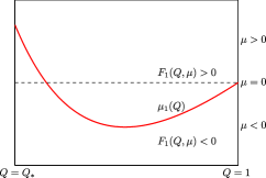
(a) The graph of $\mu_{1}(Q)$. For $Q_{*}<Q<1$, $F_{1}(Q,\mu)$ is positive in the region above the graph of $\mu_{1}(Q)$ and is negative in the region below the graph of $\mu_{1}(Q)$.

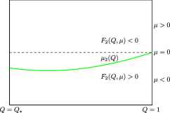
(b) The graph of $\mu_{2}(Q)$. For $Q_{*}<Q<1$, $F_{2}(Q,\mu)$ is negative in the region above the graph of $\mu_{2}(Q)$ and is positive in the region below the graph of $\mu_{2}(Q)$.

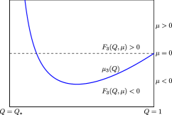
(c) The graph of $\mu_{3}(Q)$. For $Q_{*}<Q<1$, $F_{3}(Q,\mu)$ is positive in the region above the graph of $\mu_{3}(Q)$ and is negative in the region below the graph of $\mu_{3}(Q)$.

Figure 1. The graphs of $\mu_{i}(Q)$ and the signs of $F_{i}(Q,\mu)$.

Furthermore, the graphs of $\mu_{i}(Q)$, as shown in Figure 2, have the following properties.

Lemma 3.4.

Suppose that $d>0$, $n\in[2,3]$, and $c\in[1.55,n)$. Then the following are true:

1. For $i=1,2,3$, $\mu_{i}(Q)\rightarrow 0^{-}$ as $Q\rightarrow 1^{-}$.

2. For each $i=1,2,3$, $\mu_{i}(Q)$ has a unique global minimum at $Q=Q_{i}\in(Q_{*},1)$.

   1. $Q_{1}=(\frac{c}{n})^{\frac{1}{n-1}}$.

   2. $Q_{2}<Q_{1}$, and the graphs of $\mu_{1}(Q)$ and $\mu_{2}(Q)$ intersect at $Q=Q_{2}$.

   3. $\mu_{3}(Q_{3})<\mu_{1}(Q_{1})<\mu_{2}(Q_{2})<0$.

3. $F_{3}(Q_{*},\mu)=g_{3}(Q_{*})<0$ for all $\mu\in{\bf{R}}$, and $\mu_{3}(Q)\rightarrow\infty$ as $Q\rightarrow Q_{*}^{+}$.

4. $\mu_{3}(Q)<\mu_{1}(Q)$ for $Q\in(Q_{2},1)$.

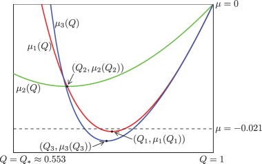
Figure 2. The graphs of $\mu_{i}(Q)$ with $d=3$, $n=2.5$, and $c=1.7$. The properties stated in Lemma 3.4 are true for all $d>0$, $n\in[2,3]$, and $c\in[1.55,n)$.

Remark 1.

With the closed-form expressions of (3.13) for $i=1,2,3$, Lemma 3.4 can be checked by elementary calculations, which are omitted. Here, we just mention the following:

1. The condition $c<n$ ensures that $Q_{1}=(\frac{c}{n})^{\frac{1}{n-1}}<1$.

2. Recall that for each $n>0$, $h_{3}(Q)$ has a unique zero at $Q=Q_{*}\in(0,1)$, which depends on $n$ only according to (3.14). The condition $c\geq 1.55$ guarantees that for any $n\in[2,3]$ and the corresponding $Q_{*}$, $F_{3}(Q_{*},\mu)=g_{3}(Q_{*})+h_{3}(Q_{*})\mu=g_{3}(Q_{*})<0$. The lower bound $1.55$ can be further reduced, but such a lower bound is necessary as $g_{3}(Q_{*})$ can become positive for some $n\in[2,3]$ if $c$ is too small (though still positive).

Recall that $Q_{r}(r)<0$ for all $r\in(0,\tau)$. By the definition (3.4) of $\tau$, one of the following three mutually exclusive cases must occur for a solution $Q(r)$ of the IVP (3.3):

1. $Q_{\tau}<Q_{*}$. This happens if and only if there exists a finite $r_{*}\in(0,\tau)$ (with either $\tau$ being finite or $\tau=\infty$) such that $Q(r_{*})=Q_{*}$ and $Q_{r}(r)<0$ for all $r\in(0,r_{*}]$.

2. $\tau<\infty$, and $\lim_{r\rightarrow\tau^{-}}Q(r)=Q_{\tau}\geq Q_{*}$. In this case, as $r\rightarrow\tau^{-}$, $Q_{r}(r)$ is bounded due to (3.9). In turn, we have the boundedness of $Q_{rr}(r)$ from (3.6), the boundedness of $Q_{rrr}(r)$ from (3.3a), and the boundedness of $Q_{rrrr}(r)$ after further differentiation of (3.3a). It follows that $Q(r)\in C^{3}([0,\tau])$. Thus, in this case, we actually have that $Q(\tau)=Q_{\tau}\geq Q_{*}$ and $Q_{r}(\tau)=0$.

3. $\tau=\infty$, and $\lim_{r\rightarrow\infty}Q(r)=Q_{\tau}\geq Q_{*}$.

Define the set $A$ as follows:

Definition 1.

$\mu<0$ is in the set $A$ if and only if case (i) happens for the solution $Q(r)$ of the IVP (3.3) with $Q_{rr}(0)=\mu$.

Lemma 3.5.

$A$ is open.

Proof.

If case (i) happens for $Q_{rr}(0)=\mu$, then there exists a small $\epsilon>0$ such that $Q_{\tau}<Q(r_{*}+\epsilon)<Q_{*}$ and $Q_{r}(r)<0$ for all $r\in(0,r_{*}+\epsilon]$ with $r_{*}+\epsilon<\tau$. Then by Lemma 3.1, there is a $\delta>0$ such that for each $\mu^{\prime}\in(\mu-\delta,\mu+\delta)$, the solution is below $Q_{*}$ at $r=r_{*}+\epsilon$ and the derivative is negative for all $r\in(0,r_{*}+\epsilon]$. This implies that case (i) also happens for all $\mu^{\prime}\in(\mu-\delta,\mu+\delta)$. Then $(\mu-\delta,\mu+\delta)\subseteq A$ by the definition of $A$. ∎

Lemma 3.6.

$(-\infty,\mu_{3}(Q_{3}))\subseteq A$.

Proof.

We show by contradiction that cases (ii) and (iii) cannot occur if $\mu<\mu_{3}(Q_{3})$.

Suppose that case (ii) happens. By continuity, evaluating (3.12) at $r=\tau$ gives $Q_{rr}(\tau)\leq F_{3}(Q_{\tau},\mu)<0$ as $Q_{\tau}\geq Q_{*}$ and $\mu<\mu_{3}(Q_{3})$ (see Figure 1(c)). On the other hand, since $Q_{r}(r)<0$ for all $r\in(0,\tau)$ and $Q_{r}(\tau)=0$, we must have that $Q_{rr}(\tau)\geq 0$, which yields a contradiction.

Suppose that case (iii) happens. Then $Q(r)>Q_{\tau}\geq Q_{*}>0$ for all $r\in(0,\infty)$. It follows that $2F_{2}(Q(r),\mu)(Q(r))^{-n}$ is bounded for all $r\in(0,\infty)$. Then, $Q_{r}(r)$ is also bounded for all $r\in(0,\infty)$ according to (3.9). From (3.12), we have that $Q_{rr}(r)+(d-1)Q_{r}(r)/r<F_{3}(Q(r),\mu)$ for all $r\in(0,\infty)$. Then $\limsup_{r\rightarrow\infty}Q_{rr}(r)\leq F_{3}(Q_{\tau},\mu)$. As $F_{3}(Q_{\tau},\mu)<0$ for $Q_{\tau}\geq Q_{*}$ and $\mu<\mu_{3}(Q_{3})$, the estimate for $\limsup_{r\rightarrow\infty}Q_{rr}(r)$ prohibits the convergence of $Q(r)$, producing a contradiction. ∎

Lemma 3.7.

$(\mu_{2}(Q_{2}),0)\cap A=\emptyset.$

Proof.

Suppose that there exists $\mu_{s}\in(\mu_{2}(Q_{2}),0)\cap A$. Since $\mu_{s}\in A$, there exists $r_{*}\in(0,\tau)$ such that $Q(r_{*})=Q_{*}>Q_{\tau}$ and $Q_{r}(r)<0$ for all $r\in(0,r_{*}]$. By (3.9), we have that $0<Q_{r}^{2}<2F_{2}(Q,\mu_{s})Q^{-n}$ for all $Q\in[Q_{*},1)$. However, since $\mu_{s}\in(\mu_{2}(Q_{2}),0)$, there exists $Q_{s}\in(Q_{2},1)\subset(Q_{*},1)$ such that $\mu_{s}=\mu_{2}(Q_{s})$. It follows that $F_{2}(Q_{s},\mu_{s})=F_{2}(Q_{s},\mu_{2}(Q_{s}))=0$, which gives a contradiction. ∎

Define $\mu_{c}:=\sup A$. By (2c) of Lemma 3.4 and Lemmas 3.6 and 3.7, we have that

$$\mu_{c}=\sup A\in[\mu_{3}(Q_{3}),\mu_{2}(Q_{2})]<0.$$

The next lemma proves Proposition 3.2.

Lemma 3.8.

For the solution $Q(r)$ of the IVP (3.3) with $\mu=\mu_{c}$, $Q_{r}(r)<0$ for all $r\in(0,\infty)$, and $\lim_{r\rightarrow\infty}Q(r)\geq Q_{*}$.

Proof.

Since $A$ is open by Lemma 3.5, $\mu_{c}=\sup A\not\in A$. Then the only possibilities are cases (ii) and (iii). It remains to show that case (ii) does not happen.

If case (ii) happens, then $Q_{rr}(\tau)$ must be nonnegative since $Q_{r}(r)<0$ for all $r\in(0,\tau)$ and $Q_{r}(\tau)=0$. We further divide case (ii) into the following three mutually exclusive sub-cases:

1. $\tau<\infty$, $Q(\tau)=Q_{\tau}>Q_{*}$, $Q_{r}(\tau)=0$, and $Q_{rr}(\tau)>0$.

2. $\tau<\infty$, $Q(\tau)=Q_{\tau}>Q_{*}$, $Q_{r}(\tau)=0$, and $Q_{rr}(\tau)=0$.

3. $\tau<\infty$, $Q(\tau)=Q_{\tau}=Q_{*}$, and $Q_{r}(\tau)=0$.

If (ii.a) happens, we can further extend the solution. Specifically, since $Q_{r}(\tau)=0$ and $Q_{rr}(\tau)>0$, there is a small $\epsilon>0$ such that $Q(r)\geq Q_{\tau}>Q_{*}$ for all $r\in[0,\tau+\epsilon]$, $Q_{r}(r)<0$ for all $r\in(0,\tau-\epsilon]$, and $Q_{r}(\tau+\epsilon)>0$. Then by Lemma 3.1, there is a $\delta>0$ such that for each $\mu\in(\mu_{c}-\delta,\mu_{c}+\delta)$, the solution is above $Q_{*}$ for all $r\in[0,\tau+\epsilon]$ with a local minimum in the interval $[\tau-\epsilon,\tau+\epsilon]$. This implies that $(\mu_{c}-\delta,\mu_{c}+\delta)\cap A=\emptyset$ by the definition of $A$. This cannot be true since $\mu_{c}=\sup A$.

Case (ii.b) is impossible since the ODE (3.3a) with the initial condition $Q(\tau)=Q_{\tau}$, $Q_{r}(\tau)=0$, and $Q_{rr}(\tau)=0$ has a unique solution $Q(r)\equiv Q_{\tau}$.

If (ii.c) happens, then evaluating (3.12) at $r=\tau$ gives $Q_{rr}(\tau)\leq F_{3}(Q_{*},\mu_{c})=g_{3}(Q_{*})<0$. This is impossible since $Q_{rr}(\tau)$ must be nonnegative when case (ii) happens. ∎

3.2. Proof of Proposition 3.3 and Example for Exponential Convergence

First we prove:

Lemma 3.9.

If $Q_{r}(r)<0$ for all $r\in(0,\infty)$ and $\lim_{r\rightarrow\infty}Q(r)=Q_{\tau}>0$, then $\lim_{r\rightarrow\infty}Q_{r}(r)=0$ and $\lim_{r\rightarrow\infty}Q_{rr}(r)=0$.

Proof.

By the hypothesis of the lemma, we have (3.6), (3.9), and (3.12) for all $r\in(0,\infty)$ and $Q=Q(r)\in(Q_{\tau},1)$. In the limit $r\rightarrow\infty$ (and correspondingly $Q\rightarrow Q_{\tau}^{+}$), inequality (3.9) implies that $|Q_{r}|$ is bounded. Then by (3.12), there is some $M>0$ such that $Q_{rr}<M$ for all $r\in(0,\infty)$ and correspondingly for all $Q=Q(r)\in(Q_{\tau},1)$. Suppose $Q_{r}$ does not converge to $0$ as $r\rightarrow\infty$. Recall that $Q_{r}(r)<0$ for all $r\in(0,\infty)$. Then we can find an $\epsilon>0$ and a sequence $\{r_{i}>0\}_{i=1}^{\infty}$ with $r_{i}+\frac{\epsilon}{M}<r_{i+1}$ such that $Q_{r}(r_{i})<-\epsilon$ for all $i$. It follows that

$$\int_{r_{1}}^{\infty}Q_{r}dr<\sum_{i=1}^{\infty}\int_{r_{i}}^{r_{i}+\frac{\epsilon}{M}}Q_{r}dr<\sum_{i=1}^{\infty}\int_{r_{i}}^{r_{i}+\frac{\epsilon}{M}}(-\epsilon+M(r-r_{i}))dr=\sum_{i=1}^{\infty}\frac{-\epsilon^{2}}{2M}\longrightarrow-\infty.$$

This is impossible as $Q(r)$ needs to converge to $Q_{\tau}>0$. Next, taking the limit $r\rightarrow\infty$ in (3.6), we have that $Q_{rr}$ converges to a constant. Furthermore, since $Q_{r}$ converges, $Q_{rr}$ must converge to $0$ as $r\rightarrow\infty$. ∎

With this, we can now prove Proposition 3.3.

Proof.

(Proposition 3.3) Taking the limit $r\rightarrow\infty$ on both sides of (3.8), we obtain that the right-hand side of (3.8) is zero when the upper limits of the two integrals are both $Q_{\tau}$. Since $\int_{1}^{Q}=\int_{1}^{Q_{\tau}}+\int_{Q_{\tau}}^{Q}$, we have that

$$\frac{1}{2}Q^{n}Q_{r}^{2}={} \int_{Q_{\tau}}^{Q}F_{1}(q,\mu)q^{n}dq-\int_{Q_{\tau}}^{Q}\left(\frac{n}{2}\int_{1}^{q}\frac{Q_{r}^{2}}{\hat{q}^{2}}d\hat{q}+(d-1)\frac{Q_{r}}{r}\right)q^{n}dq$$

(3.15) $$>{} \int_{Q_{\tau}}^{Q}F_{1}(q,\mu)q^{n}dq-\int_{Q_{\tau}}^{Q}\left(\frac{n}{2}\int_{1}^{q}\frac{Q_{r}^{2}}{\hat{q}^{2}}d\hat{q}\right)q^{n}dq,$$

where the inequality follows from the hypothesis that $Q_{r}(r)<0$ and $Q(r)>Q_{\tau}$ for all $r\in(0,\infty)$. Differentiating (3.15) with respect to $Q$ yields that

$$\left(F_{1}(Q,\mu)-\frac{n}{2}\int_{1}^{Q}\frac{Q_{r}^{2}}{\hat{q}^{2}}d\hat{q}\right)Q^{n},$$

which is zero in the limit $Q\rightarrow Q_{\tau}^{+}$. This can be shown by taking the limit $r\rightarrow\infty$ on both sides of (3.6). Differentiating the above expression with respect to $Q$ once more gives

$$\left(\frac{d}{dQ}F_{1}(Q,\mu)-\frac{nQ_{r}^{2}}{2Q^{2}}\right)Q^{n}+\left(F_{1}(Q,\mu)-\frac{n}{2}\int_{1}^{Q}\frac{Q_{r}^{2}}{\hat{q}^{2}}d\hat{q}\right)nQ^{n-1}.$$

In the limit $Q\rightarrow Q_{\tau}^{+}$, the second part of the above expression is zero while by Lemma 3.9 the first part converges to

$$L:=\left.\frac{d}{dQ}F_{1}(Q,\mu)\right|_{Q=Q_{\tau}}=\frac{1}{Q_{\tau}^{n}}-\frac{n}{cQ_{\tau}},$$

which is positive for $Q_{\tau}<(\frac{c}{n})^{\frac{1}{n-1}}$. It follows that $\frac{1}{2}Q^{n}Q_{r}^{2}>\frac{1}{2}L(Q-Q_{\tau})^{2}>0$ for $Q(r)$ sufficiently close to $Q_{\tau}$. This implies the exponential convergence of $Q(r)$ towards $Q_{\tau}$. ∎

Below we demonstrate a way to check the conditions of Proposition 3.3 for specific values of $d$, $n$, and $c$ using a combination of analysis and numerical integration. Although we have selected some particular choices for $d$, $n$, and $c$ here, we note that this strategy is deployable for other parameter values as well. Furthermore, this strategy can be made into a computer-assisted proof if the numerical computation is done using rigorous numerics.

Example 1.

For $d=3$, $n=2.5$, and $c=1.7$, numerical integration of (3.3) provides evidence that the conditions of Proposition 3.3 hold. Thus it is believed that the monotonic solution $Q(r)$ to the IVP (3.3) with $\mu=\mu_{c}$ converges exponentially to $Q_{\tau}$ as described in Proposition 3.3.

Explanation of Example 1.

Substituting $\mu=\mu_{c}$ and taking the limit $Q(r)\rightarrow Q_{\tau}^{+}$ in (3.6), with Lemma 3.9 we obtain that

$$F_{1}(Q_{\tau},\mu_{c})=\frac{n}{2}\int_{1}^{Q_{\tau}}\frac{Q_{r}^{2}}{q^{2}}dq<0.$$

In addition, from (3.12) and Lemma 3.9 we have that

$$F_{3}(Q_{\tau},\mu_{c})>0.$$

Thus, the point $(Q_{\tau},\mu_{c})$ must lie in the region below the graph of $\mu_{1}(Q)$, where $F_{1}(Q,\mu)<0$, and above the graph of $\mu_{3}(Q)$, where $F_{3}(Q,\mu)>0$ (see Figure 1 and Figure 2). Note that item (4) of Lemma 3.4 guarantees that such a region is nonempty.

Recall that $\mu_{1}(Q)$ has a global minimum in the interval $(Q_{*},1)$ at $Q=Q_{1}=(\frac{c}{n})^{\frac{1}{n-1}}$. For $d=3$, $n=2.5$, and $c=1.7$, the minimum $\mu_{1}(Q_{1})\approx-0.02146<-0.021$ (see Figure 2). If for $\mu=-0.021$ there exists a finite $r_{*}$ such that the solution $Q(r)$ to the IVP (3.3) satisfies that $Q(r_{*})=Q_{*}$ and $Q_{r}(r)<0$ for all $r\in(0,r_{*}]$, then $\mu=-0.021\in A$ by Definition 1. It follows that $\mu_{c}=\sup A>-0.021>\mu_{1}(Q_{1})$. Since the point $(Q_{\tau},\mu_{c})$ now must also be above the line $\mu=-0.021$ in addition to being bounded between the graphs of $\mu_{1}(Q)$ and $\mu_{3}(Q)$, it can only be in either the region with $Q_{\tau}<Q_{1}=(\frac{c}{n})^{\frac{1}{n-1}}$ or the region with $Q_{\tau}>Q_{1}=(\frac{c}{n})^{\frac{1}{n-1}}$ (see Figure 2). The latter is impossible since the linearization of (3.3a) at such a $Q_{\tau}$ has oscillatory dynamics that forbid a solution from converging to $Q_{\tau}$ monotonically. Then by Proposition 3.3, exponential convergence ensues.

Finally, we present numerical evidence that for $d=3$, $n=2.5$, and $c=1.7$, the solution to the IVP (3.3) with $\mu=-0.021$ decreases monotonically and drops below $Q_{*}$ in finite $r$. We numerically integrate the ODE (3.3a). However, to circumvent the singularity at $r=0$, we first seek a series solution to the IVP (3.3) in the form of $Q(r)=1+\frac{1}{2}\mu r^{2}+\sum_{k=3}^{\infty}a_{k}r^{k}$. For $\mu=-0.021$, we obtain that

$$Q(r)\approx 1-0.0105r^{2}+0.0002194963r^{4}-0.0000027819r^{6}+O(r^{8}).$$

Evaluating the above polynomial approximation and its first and second derivatives at $r=0.01$ gives that $Q(0.01)\approx 0.9999989500$, $Q_{r}(0.01)\approx-0.0002099991$, and $Q_{rr}(0.01)\approx-0.0209997366$. Then we use these values as the initial conditions at $r=0.01$ and integrate (3.3a) using the MATLAB ode45 function with both the relative error tolerance and the absolute error tolerance set to $10^{-10}$. The plots of the numerical solutions for $Q(r)$ and $Q_{r}(r)$ are shown in Figure 3. Notice that for $r_{*}\approx 16.969$, $Q(r_{*})=Q_{*}$ and $Q_{r}(r)<0$ for all $r\in(0,r_{*}]$. ∎

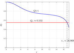
(a) $Q$ vs $r$.

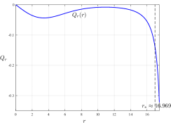
(b) $Q_{r}$ vs $r$.

Figure 3. The plots of $Q(r)$ and $Q_{r}(r)$, obtained by numerically integrating the ODE (3.3a) with the initial conditions $Q(0.01)=0.9999989500$, $Q_{r}(0.01)=-0.0002099991$, and $Q_{rr}(0.01)=-0.0209997366$. The parameter values are $d=3$, $n=2.5$, and $c=1.7$. $Q_{*}\approx 0.553$ is the unique zero in $(0,1)$ of the function $h_{3}(Q)$ given by (3.14). Note that $Q(r)$ crosses $Q_{*}$ at $r_{*}\approx 16.969$ and that $Q_{r}(r)$ is negative for all $r\in(0,r_{*}]$.

4. Discussion

In this work we have established the well-posedness of solutions to the time dependent problem (1.2), and demonstrated the existence of monotonically decaying traveling wave solutions. The major advancement here was to obtain such results in dimensions two and higher. Here, we remark on several aspects of our results.

First, our results were obtained in the “constant bulk viscosity” case and with integer nonlinearity $n$ for the permeability. This was largely to simplify presentation, and we believe our results could be extended via the same methods to the more general case,

$$\phi_{t}+\partial_{x_{d}}\left(\phi^{n}\right)-\nabla\cdot\left(\phi^{n}\nabla(\phi^{-m}\phi_{t})\right)=0,$$

allowing for non-integer exponents. Typical values of $m$ are $m\in[0,1].$

Next, with respect to the time-dependent problem, we made no mention of global-in-time results. Global-in-time results were obtained in [17] in $d=1$ for certain choices of the nonlinearity by making use of conservation laws of the form, in $d=1$,

(4.1) $$\int\frac{1}{2}|\phi^{-m}\partial_{x}\phi|^{2}+\frac{\phi^{2-n-m}-1+(n+m-2)(\phi-1)}{(n+m-1)(n+m-2)}$$

provided $n+m\neq 1,2$. An inspection of this shows that for $\phi-1\in H^{1}$, it is nonnegative and convex about the $\phi=1$ solution. Other expressions hold in the cases $n+m=1$ and $n+m=2$. For certain values of $n$ and $m$, (4.1) provides a priori an upper bound on the $H^{1}$ norm and a lower bound on $\phi$, preventing it from going to zero. This lower bound makes use of the Sobolev embedding of $H^{1}$ into $L^{\infty}$, which does not hold in higher dimensions. Since our analysis requires pointwise control of a lower bound, any analog would require a priori estimates on the higher index Sobolev spaces. Unfortunately, for general nonlinearities, no higher order conservation laws are anticipated (see [7] for some exceptions).

With regard to our main result on the solitary waves, Theorem 1.2, we note that our result is somewhat different from what might be expected by the computational geophysics community. In, for instance, [16, 15, 14, 2, 1, 30], a value of $\bar{c}>n$ is specified, and then a unimodal profile is obtained numerically that is observed to decay exponentially fast towards one. In those works, $\bar{c}$ is the only free parameter and the amplitude is unknown. Here, due to the rescaling (3.2), for each $1.55<c<n$ we obtain a unimodal profile whose amplitude is fixed at $1$, but whose limiting value $Q_{\tau}$ is unknown. Note that if we choose $\bar{q}_{0}=Q_{\tau}^{-1}$ in (3.2), then $\bar{c}=Q_{\tau}^{1-n}c$. In this case, the profile $\bar{Q}$ decays to $1$ at infinity, and the condition $Q_{\tau}<(\frac{c}{n})^{\frac{1}{n-1}}$ for exponential decay (Proposition 3.3) is exactly equivalent to $\bar{c}>n$. On the other hand, since we do not know the dependence between $Q_{\tau}$ and $c$, our result is unable to guarantee that $\bar{c}=Q_{\tau}^{1-n}c$ can be matched to a pre-specified value.

While we have not succeeded at proving exponential decay, we have provided a criterion on the solitary wave profile, which, if satisfied, ensures that such a profile decays exponentially to $Q_{\tau}$; this criterion states that if $Q_{\tau}<(\frac{c}{n})^{\frac{1}{n-1}}$, then the exponential decay does in fact occur. We have also demonstrated that for some specific parameter values, a mix of analysis and numerical evidence suggests that this criterion is satisfied.

5. Acknowledgements

We gratefully acknowledge the National Science Foundation, which has generously supported this work through grants DMS-1515849 [DMA], DMS-1409018 [GRS] and DMS-1511488 [JDW].

References

- [1] V. Barcilon and O.M. Lovera. Solitary waves in magma dynamics. J. Fluid Mech., 204:121–133, 1989.
- [2] V. Barcilon and F.M Richter. Nonlinear waves in compacting media. J. Fluid Mech., 164:429–448, 1986.
- [3] D. Bercovici, Y. Ricard, and G. Schubert. A two-phase model for compaction and damage 1. General Theory. J. Geophys. Res. B: Solid Earth, 106(B5):8887–8906, 2001.
- [4] D. Bercovici, Y. Ricard, and G. Schubert. A two-phase model of compaction and damage, 3. applications to shear localization and plate boundary formation. J. Geophys. Res., 106:8925–8940, 2001.
- [5] L.C. Evans. Partial differential equations. American Mathematical Society, 1998.
- [6] D. Gilbarg and N.S. Trudinger. Elliptic partial differential equations of second order. Springer, 2001.
- [7] S.E. Harris. Conservation laws for a nonlinear wave equation. Nonlinearity, 9(1):187–208, January 1999.
- [8] R.F. Katz, M. Spiegelman, and B.K. Holtzman. The dynamics of melt and shear localization in partially molten aggregates. Nature, 442(7103):676–679, 2006.
- [9] R.F. Katz and Y. Takei. Consequences of viscous anisotropy in a deforming, two-phase aggregate. Part 2. Numerical solutions of the full equations. J. Fluid Mech., 734:456–485, 2013.
- [10] N.V. Krylov. Lectures on elliptic and parabolic equations in Sobolev spaces. American Mathematical Society, 2008.
- [11] D. McKenzie. The generation and compaction of partially molten rock. J. Petrology, 5:713, 1984.
- [12] M. Nakayama and D.P. Mason. Rarefactive solitary waves in two-phase fluid flow of compacting media. Wave Motion, 15(4):357–392, 1992.
- [13] Y. Ricard, D. Bercovici, and G. Schubert. A two-phase model of compaction and damage, 2, applications to compaction, deformation, and the role of interfacial surface tension. J. Geophys. Res., 106:8907–8924, 2001.
- [14] David R Scott and David J Stevenson. Magma solitons. Geophysical Research Letters, 11(11):1161–1164, 1984.
- [15] D.R. Scott and D.J. Stevenson. Magma ascent by porous flow. J. Geophys. Res., 91(B9):9283, 1986.
- [16] G. Simpson and M. Spiegelman. Solitary Wave Benchmarks in Magma Dynamics. J. Sci. Comp., 49(3):268–290, 2011.
- [17] G. Simpson, M. Spiegelman, and M.I. Weinstein. Degenerate dispersive equations arising in the study of magma dynamics. Nonlinearity, 20(1):21–49, 2007.
- [18] G. Simpson, M. Spiegelman, and M.I. Weinstein. A multiscale model of partial melts: 1. Effective equations. J. Geophys. Res., 115, 2010.
- [19] G. Simpson, M. Spiegelman, and M.I. Weinstein. A multiscale model of partial melts: 2. Numerical results. J. Geophys. Res., 115(B4):B04411, 2010.
- [20] G. Simpson and M.I. Weinstein. Asymptotic Stability of Ascending Solitary Magma Waves. SIAM J. Math. Anal., 40(4):1337–1391, 2008.
- [21] Gideon Simpson. The mathematics of magma migration, 1 2008.
- [22] Gideon Simpson, Michael I Weinstein, and Philip S Rosenau. On a Hamiltonian PDE arising in magma dynamics. Discrete and Continuous Dynamical Systems Series B, 10(4):903–924, 2008.
- [23] M Spiegelman. Flow in deformable porous media. Part 1 Simple analysis. Journal Of Fluid Mechanics, 247(-1):17, 1993.
- [24] M. Spiegelman. Physics of Melt Extraction: Theory, Implications and Applications. Phil. Trans.: Phys. Sci. Engineering, 342:23, 1993.
- [25] M. Spiegelman. Geochemical effects of magmatic solitary waves - II. Some analysis. Geophys. J. International, 117(2):296–300, 1994.
- [26] Y. Takei and B.K. Holtzman. Viscous constitutive relations of solid-liquid composites in terms of grain boundary contiguity: 1. Grain boundary diffusion control model. J. Geophys. Res., 114(B6):B06205, June 2009.
- [27] Y. Takei and B.K. Holtzman. Viscous constitutive relations of solid-liquid composites in terms of grain boundary contiguity: 2. Compositional model for small melt fractions. J. Geophys. Res., 114(B6):B06206, June 2009.
- [28] Y. Takei and B.K. Holtzman. Viscous constitutive relations of solid-liquid composites in terms of grain boundary contiguity: 3. Causes and consequences of viscous anisotropy. J. Geophys. Res., 114(B6):B06207, June 2009.
- [29] Y. Takei and R.F Katz. Consequences of viscous anisotropy in a deforming, two-phase aggregate. Part 1. Governing equations and linearized analysis. J. Fluid Mech., 734:424–455, 2013.
- [30] C.H. Wiggins and M.W. Spiegelman. Magma migration and magmatic solitary waves in 3-D. Geophys. Res. Lett., 22:1289–1292, 1995.
- [31] E. Zeidler. Nonlinear functional analysis and its applications. I. Springer-Verlag, New York, 1986. Fixed-point theorems, Translated from the German by P.R. Wadsack.