Total spectral distributions from Hawking radiation

Abstract

Taking into account time-dependence of the Hawking temperature and finite evaporation time of the black hole, total spectral distributions of the radiant energy and of the number of particles have been explicitly calculated and compared to their temporary (initial) blackbody counterparts (spectral exitances).

1 Introduction

One of the most famous features of the Hawking black hole (BH) radiation is its blackbody thermal (Planckian) spectrum Hawking1974 ; hawking1975particle ; Page1976 ; Page2005 ; Harlow2016 . However, on the other hand, it is also well-known, that the BH blackbody thermality is modified in a number of ways visser2015thermality ; Dvali2016 . Actually, the shape of the BH spectrum is only approximately Planckian, with certain key modifications, especially for small BH’s. A direct consequence of the Hawking radiant flux from the BH is its evaporation Hawking1974 ; hawking1975particle , i.e., the mass $M$ of the BH monotonically decreases in time. Moreover, since the BH blackbody temperature $T_{\textrm{H}}$ (the Hawking temperature) depends on the reciprocal of $M$ (see (11)), $T_{\textrm{H}}$ is a growing function of time Hawking1974 ; hawking1975particle . The author of visser2015thermality has presented an elegant and exhaustive discussion of various modifications and limitations of the thermality of the Hawking radiation. According to visser2015thermality the Planckian shape of the Hawking spectrum will be modified by at least three distinct physical effects: greybody factors, adiabaticity constraints and available phase space. From our perspective, somewhat arbitrarily, we could add to the list the following (not quite independent, nor new) modifications of the thermality: the BH radiation lasts for a finite period of time $t_{\textrm{e}}$ (the evaporation time) Hawking1974 ; hawking1975particle , and the total number $N$ of the particles emitted by the BH is finite. Interestingly, it appears that the particles are being emitted from the BH (in a sense) rather rarely gray2016hawking . The mentioned (finite) total number $N$ (strictly speaking, its average) of particles (photons) emitted has been calculated quite recently in alonso2015entropy , and especially in muck2016hawking . The finiteness of $N$ is not quite unexpected, but it is not obvious for gapless particles, e.g. for photons. Moreover, this fact (i.e., the finiteness of $N$) could possibly also influence discussion around the BH information paradox Harlow2016 . Since we deal with a finite process ($t_{\textrm{e}}<+\infty$), and the Hawking temperature $T_{\textrm{H}}$ is a (non-constant) function of time, what could be physically more representative for the BH evaporation process than the initial or temporary blackbody spectrum expressed by the spectral radiant exitance $e_{\omega}$ (see (2)) is the total spectral distribution of energy $E_{\omega}$ coming from the total particle production from the BH. Therefore, the aim of the present work is to calculate the total spectral distribution of energy $E_{\omega}$, and also its actinometric counterpart $N_{\omega}$ (the total spectral distribution of the number of particles), both emitted during the whole BH evaporation time $t_{\textrm{e}}$. In other words, we assume complete evaporation (the final mass $M_{\textrm{f}}=0$). This assumption implicitly ignores possible modifications of the evaporation process for the temporary mass of the order of the Planck mass, when unknown quantum gravity effects should probably be taken into account. For simplicity, we also assume that at any instant of time the radiation is given by the Hawking blackbody formula for the Schwarzschild BH. Moreover, we limit our discussion to one species of massless particles, i.e., to photons. Thanks to these simplifications, we are able to express the both formulas in closed analytical forms as polylogarithm functions. The both calculated distributions are not only interesting in itself, but also they give rise to the approximate notion of the (time) average(d) temperature $\overline{T}$ (see (30) and (31)), which we aim to estimate, as a quantity alternative to the (temporary) Hawking temperature $T_{\textrm{H}}$.

According to standard terminology, the notion radiometric refers to the quantities corresponding to radiant energy, whereas the notion actinometric (photometric or photonic) refers to the quantities corresponding to the number of radiant particles (photons) stewart2012blackbody . In the case of spectral (i.e., $\omega$-dependent) quantities, the both possibilities are multiplicatively related with the Planck multiplier $\hbar\omega$. The simplest relation of this type is

$$e_{\omega}=\hbar\omega\mathcal{N}_{\omega},$$ (1)

where $e_{\omega}$ is the spectral radiant exitance, in the case of the blackbody, given by the well-known Planck law greiner1995thermodynamics (cf. Landau1969 ; Blundell2009 )

$$e_{\omega}=\frac{\hbar\omega^{3}}{4\pi^{2}c^{2}}\cdot\frac{1}{e^{\nicefrac{{\hbar\omega}}{{k_{\textrm{B}}T}}}-1}\equiv\frac{\hbar\omega^{3}}{4\pi^{2}c^{2}}\textrm{Li}_{0}\left(e^{-\frac{\hbar\omega}{k_{\textrm{B}}T}}\right),$$ (2)

and $\mathcal{N}_{\omega}$ is the corresponding spectral particle (photon) exitance assuming the standard form

$$\mathcal{N}_{\omega}=\frac{\omega^{2}}{4\pi^{2}c^{2}}\cdot\frac{1}{e^{\nicefrac{{\hbar\omega}}{{k_{\textrm{B}}T}}}-1}\equiv\frac{\omega^{2}}{4\pi^{2}c^{2}}\textrm{Li}_{0}\left(e^{-\frac{\hbar\omega}{k_{\textrm{B}}T}}\right).$$ (3)

Here, $\hbar$ is the reduced Planck constant ($h/2\pi$), $c$ — the speed of light, $k_{\textrm{B}}$ — the Boltzmann constant, $\omega$ — the angular frequency, $T$ — the blackbody temperature, and $\textrm{Li}_{0}$ is the polylogarithm function Li of the $0$th order (see Appendix). The notation assumed in the paper is not quite standard — see Chapts. 34 and 36 in 9780071629270 for standard notation.

Except where necessary, for clarity, we confine ourselves only to radiometric quantities (actinometric quantities can be easily reproduced according to (10)). Nevertheless, we aim to treat the both types of quantities equally and complementing each other.

The total radiant exitance, denoted in our paper by $e$, is given (for the blackbody) by the famous Stefan–Boltzmann law

$$e=\int_{0}^{\infty}e_{\omega}d\omega=\frac{\pi^{2}}{60}\cdot\frac{k_{\textrm{B}}^{4}}{c^{2}\hbar^{3}}T^{4}\equiv\sigma T^{4},$$ (4)

where $\sigma$ is the Stefan–Boltzmann constant, whereas the corresponding total particle (photon) exitance,

$$\mathcal{N}=\intop_{0}^{\infty}\mathcal{N}_{\omega}d\omega=\frac{\zeta\left(3\right)}{2\pi^{2}}\cdot\frac{k_{\textrm{B}}^{3}}{c^{2}\hbar^{3}}T^{3},$$ (5)

with $\zeta\left(3\right)\approx 1.20206$. For processes being considered in a finite time interval, we can introduce the notion of the total energy, expressed by integration within this time interval,

$$E=\int Ae\thinspace dt,$$ (6)

and the notion of the total number of particles,

$$N=\int A\thinspace\mathcal{N}\thinspace dt,$$ (7)

where $A$ denotes the area of the surface of the source. Analogously, the total spectral distribution of energy, we are most interested in, is defined by

$$E_{\omega}=\int Ae_{\omega}dt,$$ (8)

whereas the total spectral distribution of the number of particles defined by

$$N_{\omega}=\int A\mathcal{N}_{\omega}dt$$ (9)

is directly related to (8) by the relation (cf. (1))

$$E_{\omega}=\hbar\omega N_{\omega}.$$ (10)

2 Total number of particles

For the Schwarzschild BH, the spectral radiant exitance $e_{\omega}$, and the spectral particle (photon) exitance $\mathcal{N}_{\omega}$ is given by the standard thermodynamic formulas (2), and (3), respectively, with $T$ equal the Hawking BH temperature $T_{\textrm{H}}$, i.e.,

$$T=T_{\textrm{H}}\equiv\frac{\hbar c^{3}}{8\pi k_{\textrm{B}}GM},$$ (11)

where $G$ is the Newton gravitational constant.

Analogously, the total radiant exitance $e$, and the total particle (photon) exitance $\mathcal{N}$ is given by another couple of standard thermodynamic formulas, (4) and (5), respectively, with $T=T_{\textrm{H}}$.

The total radiant energy (see (6)) is directly given by the Einstein mass–energy equivalence formula

$$E=Mc^{2},$$ (12)

whereas the total number $N$ of particles (photons) emitted by the BH has been determined quite recently in alonso2015entropy ; muck2016hawking .

Since, in the next section, for technical reasons, we will need in our calculations the formula expressing the mass flow rate $dM/dt$ in terms of the mass $M$, involved in the derivation of the evaporation time $t_{\textrm{e}}$, we rederive it in the present section. As a byproduct of our derivation, we compute the total number $N$ of particles (photons) emitted during the whole BH evaporation process. By virtue of the equivalence formula (12), and of the Stefan–Boltzmann law (4), the mass flow rate

$$\frac{dM}{dt}=-\frac{1}{c^{2}}\frac{dE}{dt}=-\frac{1}{c^{2}}Ae=-\frac{1}{c^{2}}A\sigma T^{4},$$ (13)

where $dE/dt$ can be interpreted as the velocity of evaporation. Inserting to (13) the standard BH horizon surface area formula

$$A=\frac{16\pi G^{2}}{c^{2}}M^{2},$$ (14)

and the Hawking BH temperature formula (11), we obtain the differential equation expressing the mass flow rate in terms of $M$

$$\frac{dM}{dt}=-\frac{\hbar c^{4}}{15\cdot 2^{10}\pi G^{2}}M^{-2}.$$ (15)

This equation yields the evaporation time

$$t_{\textrm{e}}=\frac{5\cdot 2^{10}\pi G^{2}}{\hbar c^{4}}M_{0}^{3},$$ (16)

where $M_{0}$ denotes the initial mass of the BH.

As a byproduct of our derivation (15), we can now calculate the total number $N$ of particles (photons) emitted during the whole BH evaporation process. To this end, we will apply a technical trick which consists in using the chain rule to the number flow rate (given by differential form of (7)), and next performing some further formal manipulations (insertions). Thus, first, we get

$$\frac{dN}{dt}=\frac{dN}{dM}\frac{dM}{dt}=A\mathcal{N}.$$ (17)

Inserting the mass flow rate (15) into the central part of (17), and next the area formula (14), the total particle exitance (5), the Hawking temperature (11) into the RHS of (17), respectively, after simple rearrangements, we obtain, in agreement with earlier derivations given in alonso2015entropy ; muck2016hawking , the differential equation

$$\frac{dN}{dM}=-\frac{240\thinspace\zeta\left(3\right)G}{\pi^{3}\hbar c}M,$$ (18)

where the Riemann zeta function $\zeta\left(3\right)\approx 1.202$. The solution of (18) yields the total number of particles emitted

$$N=\frac{120\thinspace\zeta\left(3\right)G}{\pi^{3}\hbar c}M_{0}^{2}.$$ (19)

Thus, the total radiant energy $E$, and the total number $N$ of particles (photons) emitted, both related to complete evaporation, are determined.

3 Total spectral distributions

The total spectral distribution $E_{\omega}$ of the total energy $E$ emitted during the whole BH evaporation process is determined by the spectral power (given by differential form of (8))

$$\frac{dE_{\omega}}{dt}=Ae_{\omega},$$ (20)

or, equivalently, using the chain rule as a technical trick,

$$\frac{dE_{\omega}}{dM}=\left(\frac{dM}{dt}\right)^{-1}Ae_{\omega}.$$ (21)

Making use of the mass flow rate formula (15), the area formula (14) and the Planck law (2), we obtain from (21) the (differential) element of the total spectral distribution of energy

$$dE_{\omega}=-\frac{15\cdot 2^{12}G^{4}}{c^{10}}\omega^{3}M^{4}\textrm{Li}_{0}\left(e^{-\frac{8\pi G}{c^{3}}\omega M}\right)dM,$$ (22)

or in terms of an (auxiliary) dimensionless BH mass

$$x\equiv\frac{8\pi G}{c^{3}}\omega M,$$ (23)

$$dE_{\omega}=-\frac{15c^{5}}{8\pi^{5}G}\omega^{-2}x^{4}\textrm{Li}_{0}\left(e^{-x}\right)dx.$$ (24)

Now, we should integrate out the RHS of (24) with respect to the mass $x$ over the finite mass interval $\left[x_{0},0\right]$, corresponding to the total (initial) mass $M_{0}$ of the BH, where

$$x_{0}\equiv\frac{8\pi G}{c^{3}}\omega M_{0}$$ (25)

is a dimensionless frequency. Utilizing the integral identity (36), we obtain our final formula for the total spectral distribution of total energy

$$E_{\omega}=\frac{45c^{5}}{\pi^{5}G}\omega^{-2}\left[\zeta\left(5\right)-\sum_{k=0}^{4}\frac{x_{0}^{4-k}}{\left(4-k\right)!}\textrm{Li}_{k+1}\left(e^{-x_{0}}\right)\right].$$ (26)

Here, the Riemann zeta function $\zeta\left(5\right)$ ($\approx 1.03693$) is the only contribution from $0$ (the upper limit of the integral, corresponding to the final mass $M_{\textrm{f}}=0$). More precisely, for $k=4$ in the sum in the identity (36) (see the Riemann zeta function identity (35)),

$$\lim_{x\rightarrow 0}\textrm{Li}_{4+1}\left(e^{-x}\right)=\textrm{Li}_{5}\left(1\right)=\zeta\left(5\right),$$ (27)

and there are no other contributions to (36) from 0. In fact, for $k=1,2,3,$ we have (see (35))

$$\lim_{x\rightarrow 0}x^{4-k}\textrm{Li}_{k+1}\left(e^{-x}\right)=\left.x^{4-k}\zeta\left(k+1\right)\right|_{x=0}=0,$$ (28)

whereas for $k=0$ (see (34))

$$\lim_{x\rightarrow 0}x^{4}\textrm{Li}_{1}\left(e^{-x}\right)=-\lim_{x\rightarrow 0}x^{4}\ln\left(1-e^{-x}\right)=0.$$ (29)

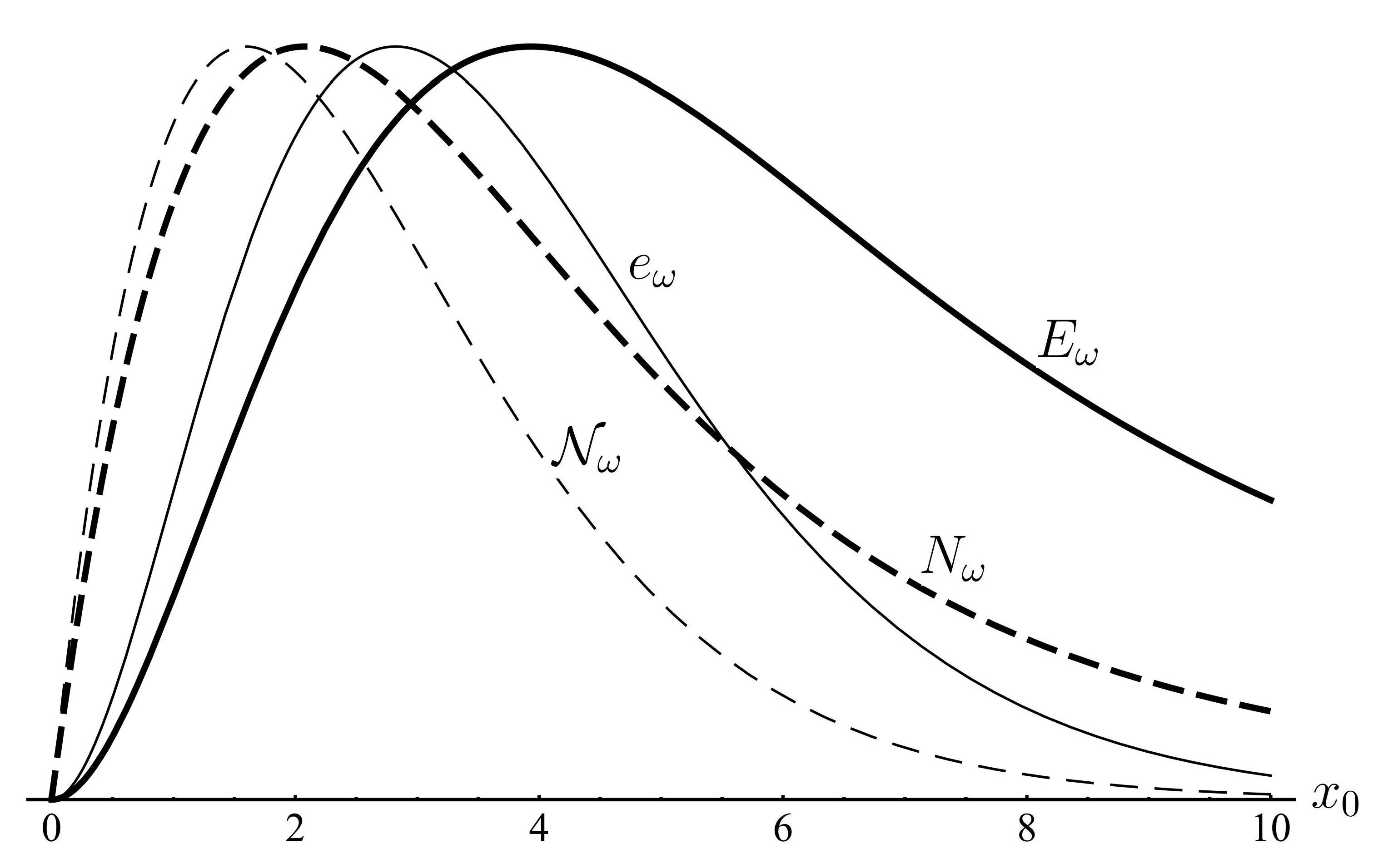
$F_{\omega}=$	$e_{\omega}$	$\mathcal{N}_{\omega}$	$E_{\omega}$	$N_{\omega}$
$x_{\textrm{max}}\left(F_{\omega}\right)=$	$2.82144$	$1.59362$	$3.93334$	$2.07408$

Figure 1: All the four spectral functions discussed in the paper. Since the functions are expressed in different physical units, they have been all normalized to a common “one”, by convention, and the vertical axis has been removed. Numerical values, denoted by $x_{\textrm{max}}\left(F_{\omega}\right)$, of the dimensionless frequency $x_{0}$ defined in (25), corresponding to maxima of the spectral functions are given in the table above.

4 Discussion and conclusions

It seems that the best way to discuss the shape of the total spectral distributions $E_{\omega}$ and $N_{\omega}$ for the BH, given by (26) and (10), is by comparison to analogous temporary (initial) spectral exitances for the corresponding blackbody, i.e., to $e_{\omega}$ and $\mathcal{N}_{\omega}$, respectively. Differences and similarities between respective spectral functions can be directly observed in Fig. 1. Their maxima, $x_{\textrm{max}}\left(F_{\omega}\right)$, have been numerically determined, and they are given in the table in Fig. 1. In particular, we can observe that the values of the arguments for the maxima of the total distributions are (a bit) greater than the values of the arguments for the maxima of their temporary (initial) blackbody counterparts, i.e., $x_{\textrm{max}}\left(E_{\omega}\right)>x_{\textrm{max}}\left(e_{\omega}\right)$ and $x_{\textrm{max}}\left(N_{\omega}\right)>x_{\textrm{max}}\left(\mathcal{N}_{\omega}\right)$. Since the shapes of the total spectral distributions in their central parts (in particular, we can ignore IR and UV tails, which are a bit unphysical, see visser2015thermality ) are similar to their blackbody counterparts, making use of the above mentioned shifts of the maxima, we can introduce the approximate notion of the (time) average(d) temperature $\overline{T}$. More precisely, actually we deal with two a bit differing average(d) temperatures. One temperature, $\overline{T}_{E}$, corresponds to energy, and the second one, $\overline{T}_{N}$, corresponds to the number of particles, respectively, and they both are multiplicatively related to $T_{\textrm{H}}$. Namely,

$$\overline{T}_{E}\equiv\dfrac{x_{\textrm{max}}\left(E_{\omega}\right)}{x_{\textrm{max}}\left(e_{\omega}\right)}T_{\textrm{H}}\approx 1.39409\cdot T_{\textrm{H}},$$ (30)

and

$$\overline{T}_{N}\equiv\dfrac{x_{\textrm{max}}\left(N_{\omega}\right)}{x_{\textrm{max}}\left(\mathcal{N}_{\omega}\right)}T_{\textrm{H}}\approx 1.30149\cdot T_{\textrm{H}},$$ (31)

respectively. Here, the Hawking temperature $T_{\textrm{H}}$ is the temporary blackbody temperature of the initial BH. Thus, on average, the BH temperature is some $1.3$–$1.4$ times greater than its initial Hawking temperature $T_{\textrm{H}}$.

Since the Hawking radiation of a BH is a blackbody radiation with the temperature $T_{\textrm{H}}$ which changes in time, and the BH evaporation time $t_{\textrm{e}}$ is finite (see (16)), in this paper, we have focused on the total spectral distributions corresponding to the complete evaporation process, rather than on temporary (initial) blackbody quantities (spectral exitances). The total spectral distribution of energy, $E_{\omega}$, and the total spectral distribution of the number of particles, $N_{\omega}$, have been explicitly calculated and compared to their initial blackbody counterparts.

Appendix

The polylogarithm function (polylogarithm, in short) has already proved to be very useful in the context of problems of conventional blackbody radiation. In particular, exact formulas for blackbody radiation within a given finite spectral band elegantly express in terms of polylogarithms stewart2012blackbody .

For real or complex $s$ and $z$ the polylogarithm $\textrm{Li}_{s}(z)$ is defined by olver2010nist

$$\textrm{Li}_{s}\left(z\right)\equiv{\displaystyle\sum_{k=1}^{\infty}\frac{z^{k}}{k^{s}}.}$$ (32)

For each fixed complex $s$ the series defines an analytic function of $z$ for $\left|z\right|<1$. The series also converges when $\left|z\right|=1$, provided that $\Re s>1$. For other values of $z$, $\textrm{Li}_{s}(z)$ is defined by analytic continuation.

In particular,

$$\textrm{Li}_{0}\left(z\right)=\frac{z}{1-z},$$ (33)

and

$$\textrm{Li}_{1}\left(z\right)=-\ln\left(1-z\right).$$ (34)

The special case $z=1$ is the Riemann zeta function:

$$\zeta\left(s\right)=\textrm{Li}_{s}\left(1\right).$$ (35)

Integrating by parts, we can verify the following very useful in our calculations integral identity stewart2012blackbody

$$\int x^{n}\textrm{Li}_{0}\left(e^{-x}\right)dx=\textrm{const}.-n!\sum_{k=0}^{n}\frac{x^{n-k}}{\left(n-k\right)!}\textrm{Li}_{k+1}\left(e^{-x}\right),$$ (36)

valid for any non-negative integer $n$.

References

- (1) S.W. Hawking, Nature 248(5443), 30 (1974)
- (2) S.W. Hawking, Commun. Math. Phys. 43(3), 199 (1975). DOI 10.1007/BF02345020
- (3) D.N. Page, Physical Review D 13(2), 198 (1976)
- (4) D.N. Page, New J. Phys. 7, 203 (2005). DOI 10.1088/1367-2630/7/1/203
- (5) D. Harlow, Rev. Mod. Phys. 88(1), 015002 (2016). DOI 10.1103/RevModPhys.88.015002
- (6) M. Visser, J. High Energy Phys. 2015(7), 9 (2015). DOI 10.1007/JHEP07(2015)009
- (7) G. Dvali, Fortsch. Phys. 64, 106 (2016). DOI 10.1002/prop.201500096
- (8) A.V.B. Finnian Gray, Sebastian Schuster, M. Visser, Classical Quantum Gravity 33(11), 115003 (2016). DOI 10.1088/0264-9381/33/11/115003. URL http://stacks.iop.org/0264-9381/33/i=11/a=115003
- (9) A. Alonso-Serrano, M. Visser, ArXiv e-prints (2015)
- (10) W. Mück, The European Physical Journal C 76(7), 374 (2016). DOI 10.1140/epjc/s10052-016-4233-3
- (11) S.M. Stewart, J. Quant. Spectrosc. Radiat. Transfer 113(3), 232 (2012). DOI 10.1016/j.jqsrt.2011.10.010. URL http://www.sciencedirect.com/science/article/pii/S0022407311003736
- (12) W. Greiner, L. Neise, H. Stöcker, Thermodynamics and Statistical Mechanics. Classical Theoretical Physics (Springer New York, 1995). DOI 10.1007/978-1-4612-0827-3
- (13) L.D. Landau, E.M. Lifshitz, Statistical Physics: V. 5: Course of Theoretical Physics (Pergamon press, 1969)
- (14) S.J. Blundell, K.M. Blundell, Concepts in thermal physics (OUP Oxford, 2009)
- (15) M. Bass, C. DeCusatis, J.M. Enoch, V. Lakshminarayanan, G. Li, Handbook of Optics, Third Edition Volume II: Design, Fabrication and Testing, Sources and Detectors, Radiometry and Photometry (McGraw-Hill Education, LLC CoreSource, 2009). URL http://www.ebook.de/de/product/15187214/michael_bass_casimer_decusatis_jay_m_enoch_vasudevan_lakshminarayanan_guifang_li_handbook_of_optics_third_edition_volume_ii_design_fabrication_and_testing_sources_and_detectors_radiometry_and_photometry.html
- (16) T. Apostol, Zeta and Related Functions (Cambridge University Press, 2010), chap. 25, pp. 601–616