A Markov State Modeling analysis of sliding dynamics of a 2D model

Abstract

Non-equilibrium Markov State Modeling (MSM) has recently been proposed [Phys. Rev. E 94, 053001 (2016)] as a possible route to construct a physical theory of sliding friction from a long steady state atomistic simulation: the approach builds a small set of collective variables, which obey a transition-matrix based equation of motion, faithfully describing the slow motions of the system. A crucial question is whether this approach can be extended from the original 1D small size demo to larger and more realistic size systems, without an inordinate increase of the number and complexity of the collective variables. Here we present a direct application of the MSM scheme to the sliding of an island made of over 1000 harmonically bound particles over a 2D periodic potential. Based on a totally unprejudiced phase space metric and without requiring any special doctoring, we find that here too the scheme allows extracting a very small number of slow variables, necessary and sufficient to describe the dynamics of island sliding.

I Introduction

Sliding friction between solid bodies, among the most basic and pervasive phenomena in physics and in our everyday experience, can be measured, simulated but – disappointingly – not yet formulated theoretically. By that we mean that even in the purely classical sliding of a body on another there is no unprejudiced way of identifying and determining a handful of variables (as opposed to the $\sim{10}^{23}$ atomic coordinates and velocities) that obey a well defined equation of motion describing the essence of the frictional process. The burgeoning area of nanofriction Vanossi et al. (2013), where realistic simulations are often possible, has made if anything this theoretical vacuum even more blatant. In a recent pubblication we proposed Pellegrini et al. (2016) that Markov State modeling (MSM) – a probabilistic approach commonly applied to characterize the kinetics of systems characterized by an equilibrium measure Noé et al. (2009); Schwantes et al. (2014); Noé and Nüske (2013); Bowman et al. (2014); Schütte and Sarich (2015) – can be extended and used for the strongly non-equilibrium, non–linear problem of sliding friction. The approach was demonstrated in a simple 1D toy model, a 10-atom Frenkel Kontorova model Frenkel and T.A. Kontorova (1938) where, despite the difficulty represented by a time–growing phase space, non-equilibrium MSM was shown to describe adequately the forced dynamics of steady-state sliding friction. The probabilistic analysis of a long steady-state frictional simulation and the choice of a metric led to the recognition of Markovian evolution in phase space, to the identification of a few slow collective variables (“excitations”) describing the events occurring in the course of sliding, and to the construction of a transfer–matrix–dictated model of the time evolution of probabilities. This approach represents in our view a first step towards a theory of friction, and a methodological advance of very significant importance.

Here we showcase the first application of the MSM approach to a more realistic frictional system. We choose for this purpose the sliding of a two-dimensional (2D) island of more than $1000$ particles, harmonically interacting at a spacing that is incommensurate with respect to a periodic 2D substrate potential. We consider different sliding regimes, including the “superlubric” and, at the opposite limit, the pinned regime. The results are rewarding: firstly, and most importantly, MSM again identifies an extremely small set of significant variables, despite the totally generic choice of metric and the much larger dimensionality of the phase space in which the original model is defined. This handful of variables in turn describes without any built-in prejudice the main slow time-dependent frictional events, including superlubric soliton flow and atomic stick-slip frictional sliding of the island, in the two extreme and opposite regimes of weak and strong potential.

II Markov State Modeling

The Markov State Modeling procedure starts from a classical molecular dynamics simulation of the sliding system, long enough to explore all relevant configurations in phase space a sufficiently large number of times. Structurally similar configurations are then grouped in a finite number of microstates, which will serve as a basis, through a clustering (such as k–means Pérez-Hernández et al. (2013)) or geometric technique. This partitioning requires a metric in phase space to quantify the similarity between configurations: the quality of the partition will generally depend on this choice, to be made with utmost physical care. While in real world applications it is considered mandatory to define the metric in a relevant subset of the coordinates (for example, the coordinates of the solute), we will show that, in the specific system considered in this work, one can carry on the procedure even using a “blind” metric, defined taking into account all the cooordinates of the system.

In equilibrium settings, the transition probability matrix between pairs of microstates (in a time $\tau$) would be equivalent to a hermitian matrix (on account of detailed balance) and have a unique eigenvalue equal to one, whose eigenvector represent the equilibrium distribution, and all other real eigenvalues smaller than one. The eigenvectors of eigenvalues closest to one are associated with slow modes of the system evolution, while the smaller eigenvalues correspond to fast motions, expected to be increasingly irrelevant. A clear gap between high and low eigenvalues leads to a natural dimensional reduction Deuflhard and Weber (2005); Weber and Kube (2005).

To study non-equilibrium problems such as friction, this procedure has been modified in several key points: the frictional dynamics does not reach an equilibrium, but instead reaches a steady state where the configuration space grows (approximately) linearly with the simulation time, making sampling and clustering problematic. The solution we proposed is dividing the evolution in intervals, still long enough to be deemed equivalent between them, so that results from each interval can be cumulated on top of one another. Stability of the results against extension of the time interval indicates the validity of the procedure. Care should be taken in dealing with the transition probability matrix from this steady–state evolution under forcing, which is non-hermitian Pellegrini et al. (2016). Moreover, since the phase space metric contains a large number of microscopic variables, we do not build microstates by the tessellation techniques used in standard MSM Prinz et al. (2011), but use instead a recently proposed clustering algorithm Rodriguez and Laio (2014), which associates a microstate to each meaningful peak of the probability distribution in the coordinate space associated with the metric.

The main goal of this contribution is demonstrating that this procedure works for a much more realistic model than the one considered in ref. Pellegrini et al. (2016): the sliding of a 2D Frenkel Kontorova island including approximately 1000 atoms on a periodic incommensurate potential.

III The 2D Frenkel-Kontorova model

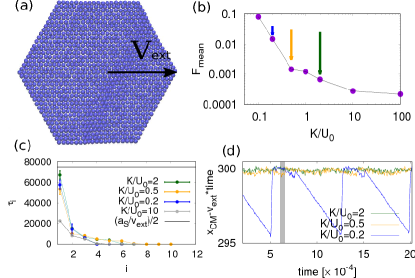
Figure 1: (a) Schematic of the Frenkel-Kontorova island sliding on a generic 2D incommensurate triangular potential. (b) Average friction force in the steady state regime for simulations with varying ratio $K/U_{0}$, highlighting the transition from free sliding to stick–slip. The arrows indicate the sample parameters chosen to compare the results of our method, with a color code we will keep throughout all figures. (c) Slowest timescales after transition matrix diagonalization for the different regimes. The full line represents half of the time required for the external force to move the particles to successive potential minima. (d) Sample evolution for the different regimes: we show the deviations of the center of mass positions from the free sliding corresponding to an infinitely stiff island. The vertical dashed lines are spaced like the time lag $\tau=1100$ chosen to build the MSM to represent sampled configurations.

Our present study focuses on a two-dimensional FK model Braun and Kivshar (1998), Fig. 1(a). We consider a hexagonal island of $N=1027$ classical particles, internally arranged as a triangular lattice, dragged by a force applied on the center of mass, which causes it to slide over a triangular potential $V(x,y)=U_{0}\left[2\cos\left(\frac{2\pi x}{a_{S}}\right)\cos\left(\frac{2\pi y}{\sqrt{3}a_{S}}\right)+\cos\left(\frac{4\pi y}{\sqrt{3}a_{S}}\right)\right]$. Nearest neighbor harmonic springs of stiffness $K$ link the particles of mass $m$ and positions $\mathbf{r}_{i}=(x_{i},y_{i})$ whose equilibrium spacing $a_{H}$ is incommensurate with the periodic potential: $a_{S}/a_{H}\sim 1.07$. Each particle is dragged by a spring of constant $\kappa$ moving with constant velocity $v_{{\rm ext}}$. Particle motion obeys an overdamped Langevin dynamics (large damping $\gamma$), in a bath of inverse temperature $\beta=1/k_{B}T$:

$$\begin{array}[]{rcl}\mathbf{r}_{l}^{t+dt}&=&\displaystyle\mathbf{r}_{l}^{t}+\left[\frac{1}{\gamma m}\nabla V(\mathbf{r}_{l}^{t})+\frac{\kappa}{\gamma m}\left(v_{\rm ext}t-\frac{1}{N}\underset{j}{\sum}x_{j}^{t}\right)+\right.\\ &&\displaystyle\left.-\frac{K}{\gamma m}\sum_{j\in\mathrm{NN}}(\mathbf{r}_{l}^{t}-\mathbf{r}_{j}^{t})\right]dt+\sqrt{\frac{2dt}{\gamma m\beta}}\mathbf{f}^{t},\end{array}$$ (1)

where $\mathbf{f}^{t}$ is an uncorrelated Gaussian distribution and $dt$ is the elementary time step (here $dt=0.1$, $m=1$, $\gamma=1$, $\beta=100$, $\kappa=0.01$, $v_{\rm ext}=0.0001$).

In a temperature and parameter regime where the island does not rotate, its sliding mechanics retains some similarity to 1D sliding Braun and Kivshar (1998). In the weak potential limit the bulk of the island, characterized by weak solitons (small deviations of the interparticle distance from the equilibrium value) which form a moiré pattern over the incommensurate potential, is structurally lubric (“superlubric”). Upon sliding in this regime the solitons flow unhindered, and the only source of pinning and static friction is actually provided by the island edge Varini et al. (2015). In the opposite strong potential limit the solitons, no longer weak, are strongly entrenched, and the whole island is pinned, with a bulk static friction independent of edges. Under the external spring–transmitted force, the island sliding in this regime will alternate long “sticking” periods during which particles are close to their respective potential minima, to fast slips during which one or more lattice spacings are gained. This kind of atomic stick–slip motion is well established for, e.g., the sliding of an Atomic Force Microscope tip on a crystal surface Vanossi et al. (2013) – of course involving in that case three-dimensional displacements of larger complexity. A slip event always involves the flow of either pre–existing solitons or of newly created ones that enable the system to slide faster.

Our input for the MSM procedure is a long steady-state trajectory of the island motion, obtained by integrating these equations for $\sim{10}^{8}$ timesteps for a slow external velocity, but far from the linear response regime. Values of $K/U_{0}$ were chosen so as to straddle between and beyond the weak ($K/U_{0}\geq 2$) and strong ($K/U_{0}\leq 0.2$) potential regimes.

The average friction force $F_{\rm mean}=\kappa\left\langle v_{ext}t-\frac{1}{N}\sum_{l}x_{l}\right\rangle$ obtained from the simulation as a function of the ratio $K/U_{0}$ can be seen in Fig. 1(b), where the crossover from a superlubric to a pinned regime is clearly reflected. We focus our study on three different values of the parameters representative of these different regimes, as can be hinted by looking at the evolution of the position of the center of mass shown in Fig. 1(d).

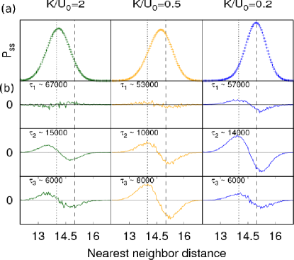
Figure 2: (a) Steady state probability distribution of the nearest neighbor distances for the three regimes. Vertical dotted lines represent the rest interparticle (“harmonic”) distance, while the dashed ones the substrate lattice spacing. (b) The perturbations $g_{i}$ (see Eq. 4) estimated for the first three excited states. The observable $O$ in Eq. 4 is here the nearest neighbor distance. To compute $P(O|\alpha)$ 100 intervals have been chosen.

IV Implementing the frictional MSM

The protocol begins by defining a metric, measuring distances between configurations in phase space. Since we want to remain as unprejudiced as possible, we adopt the simplest, most generic and bias–free metric, and define the distance between two configurations $s$ and $t$ as:

$$d_{st}=\left[({\mathbf{r}}^{s}_{\rm CM}-{\mathbf{r}}^{t}_{\rm CM})_{\text{mod }2}\right]^{2}+\left[\overset{N}{\underset{l=1}{\sum}}({\mathbf{r}}^{s}_{l}-{\mathbf{r}}^{t}_{l})_{\text{mod }2}\right]^{2}.$$ (2)

The microstates were built using the Density Peak algorithm Rodriguez and Laio (2014). This approach requires only defining a distance between the configurations, here estimated using Eq. 2. Based on this definition, the approach automatically finds the peaks in the probability distribution in the space of the coordinates in which the distance is defined. Here, following our previous work Pellegrini et al. (2016), we identify the microstates used for building the MSM with the density peaks.

We used samples of $N_{\rm conf}\sim{10}^{4}$ configurations (separated by the lagtime $\tau$) and clustered them using the metric (2). The order of magnitude of the lagtime $\tau$ has been chosen in order to describe the stick (and slip) events of the system. The optimal lagtime $\tau=1100$ was determined after some convergence checks resembling those carried out in the previous work Pellegrini et al. (2016): In particular, we verified that the relevant timescales stay within the statistical error in Fig. 1 when doubling or halving the lagtime. We also verified that by using the Core Set MSM approach Schutte2011 the influence of the time lag on the timescales is further reduced. This indicates that we are indeed far from the non-Markovian regime.

Given these $\{c_{\alpha},\alpha=1,\dots,n_{c}\}$ microstates, we can construct a discretized, coarse–grained Transfer Operator (TO) Bowman et al. (2014): if $\Pi^{\tau}(X\rightarrow X^{\prime})$ is the probability to go from a configuration $X$ at time $t$ to $X^{\prime}$ at time $t+\tau$, a finite $n_{c}\times n_{c}$ Transfer Matrix (TM) can be built by estimating the probability to go from $c_{\alpha}$ to $c_{\beta}$ in time $\tau$: $\Pi_{\alpha\beta}^{\tau}=\int_{X\in c_{\alpha}}\int_{X^{\prime}\in c_{\beta}}{\rm d}X{\rm d}X^{\prime}P(X)\Pi^{\tau}(X\rightarrow X^{\prime})$. This TM contains less detail than $\Pi^{\tau}$, but it can be sampled in finite time. In principle, $\Pi_{\alpha\beta}^{\tau}$ depends on the choice of $\tau$, but an optimal value for this parameter can be chosen. We call $\{\lambda_{i}\}$ the eigenvalues of the TM and $\{\vec{\chi}_{i}\}$ its left eigenvectors. Since detailed balance does not hold, the TM is not symmetric and the eigenvalues can be complex, however $\left|\lambda_{i}\right|\leq 1$ is still guaranteed; the eigenvalue of largest modulus is still $1$ and unique if the evolution is ergodic. The eigenvector $\vec{\chi}_{0}$ represents the steady state distribution, while the eigenvectors $\vec{\chi}_{i}$ with $\left|\lambda_{i}\right|\simeq 1$ form the so–called Perron Cluster Deuflhard and Weber (2005). They characterize the long–lived perturbations to the steady state, decaying with characteristic times $\tau_{i}=-\tau/\ln\left|\lambda_{i}\right|\gg\tau$, while oscillating with period $\tau/\arctan({\rm Im}\lambda_{i}/{\rm Re}\lambda_{i})$.

To better characterize the eigenmodes $\chi_{i}$ it is useful to consider a system prepared in the mixed state $P_{\alpha}^{0}$ (probability vector to be in $c_{\alpha}$) at $t=0$ and the evolution of the probability distribution $P\left(O,t\right)$ of an observable $O$ as a function of time. We have:

$$P\left(O,t\right)=P^{\rm ss}\left(O\right)+\sum_{i>0}f_{i}g_{i}\left(O\right)e^{-t/\tau_{i}},$$ (3)

where $f_{i}=\sum_{\alpha}\chi_{i}^{\alpha}P^{0}_{\alpha}/P^{\rm ss}_{\alpha}$ accounts for the initial condition and

$$g_{i}\left(O\right)=\sum_{\alpha}\chi_{i}^{\alpha}P(O|\alpha),$$ (4)

where $P(O|\alpha)$ is the probability distribution of $O$ in microstate $\alpha$, $P^{{\rm ss}}(O)=g_{0}(O)$ the steady state distribution of $O$, and $P_{\alpha}^{{\rm ss}}$ the steady state probability to visit microstate $\alpha$. The $g_{i}(O)$ for $i>1$ represent “perturbations” of $P^{{\rm ss}}(O)$, each decaying within the lifetime $\tau_{i}$. While the expansion (3) is meaningful only for a given starting configuration, the analysis of the shape of these functions (regardless of their amplitude) provides a direct insight into the nature of the slow eigenmodes. One can therefore turn back to observables deemed relevant in the original system and estimate their influence in the relevant dynamical modes of the system in order to gain insight on their characteristics.

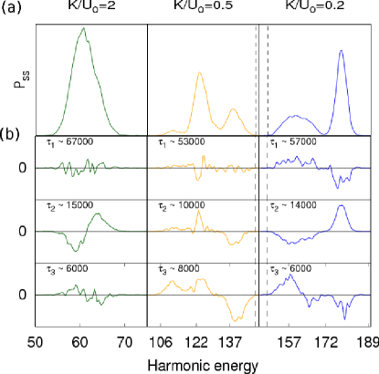
Figure 3: (a) Steady state probability distribution of the harmonic energy for the three regimes. The vertical dashed lines represent the harmonic energy for an island completely relaxed to the substrate lattice spacing. In this case we applied a running average to the data, both for the steady–state distribution and the corrections. The switch from a single peak of the hard island to a multiplicity of peaks for the medium to soft island is a direct evidence of the more elaborate sliding dynamics of the latter. (b) The perturbations $g_{i}$ (see Eq. 4) estimated for the first three excited states. The observable $O$ in Eq. 4 is here the harmonic energy. To compute $P(O|\alpha)$ 100 intervals have been chosen.

V Observables

We apply the described procedure to three evolutions of our model characterized by different parameters $K/U_{0}$ as indicated in Fig. 1(b). The time corresponding to the first largest eigenvalue (computed from the real part of the eigenvalues, besides the eigenvalue $0$ associated with the steady–state, while the imaginary part is much smaller and has been ignored) can be seen in Fig. 1(c): for all cases we find that the first implied timescale is approximately equal to $6\times{10}^{4}$, corresponding to roughly half the time $a_{S}/v_{\rm ext}$ required on average to move by one lattice spacing. This is consistent with the interpretation of the slowest mode as being related to the movement from one local minimum of the substrate to the next. We notice that in the more extreme case $K/U_{0}=10$ the first relaxation time is faster, since the island is stiff the substrate does not play a role. The successive timescales are almost an order of magnitude faster, and further insight is required for their interpretation. We will presently analyze the $g$ functions of some relevant physical observables of this frictional system, in order to characterize these rapidly decaying states.

V.1 Nearest neighbour distance

As a first observable we consider the nearest neighbor distance between all particle pairs. The steady–state distributions (see Fig. 2(a)) show the expected trend: while the $K/U_{0}=2$,case has a peak centered on the harmonic equilibrium distance reflecting the hard island’s nature during structurally lubric sliding Vanossi et al. (2013), the opposite case $K/U_{0}=0.2$ is centered on a distance commensurate with the substrate, reflecting the soft island’s strong adhesion to the external potential. For $K/U_{0}=0.5$ the situation is intermediate. The excited states complete this description (see Fig. 2(b)): the first excited states show little correction to the steady–state distribution, as the change of a whole lattice spacing has only a minor influence on the nearest neighbor distribution, while the second and third excited states display a significant change. Indeed, the latter correspond to internal relaxations of the island not associated with the collective sliding. In the specific case these corrections are related to the formation/destruction of incommensurate solitons induced on the island by the external potential Varini et al. (2015).

This observable lacks the ability to clearly distinguish between the excited states. We therefore considered a more extensive observable, able to highlight more differences.

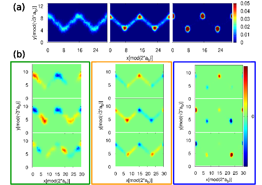
Figure 4: (a) Steady state 2D probability distribution of all single particle positions (excluding edges) for the three regimes. Position along x and y is taken modulus 1 and 2 lattice spacings, respectively. The zig-zag pattern reflects the motion of the whole which, while pulled along $X$, moves between neighboring potential minima that are $\pm 60^{\circ}$ off. (b) The perturbations $g_{i}$ (see Eq. 4) estimated for the first three excited states. The observable $O$ in Eq. 4 is here the single particle positions. Note the evolution for decreasing $K/U_{0}$, from smooth flow to sharp hopping betweem minima. To compute $P(O|\alpha)$ 100 intervals have been chosen for x and 50 for y.

V.2 Harmonic energy

We now consider the distribution of the total harmonic energy of the island $\frac{K}{2}\langle\sum_{\langle i,j\rangle\in\mathrm{NN}}(\mathbf{r}_{i}^{t}-\mathbf{r}_{j}^{t})^{2}\rangle$. Fig. 3(a) shows the steady–state distributions, clearly highlighting the richer information encoded by this observable. In the stiff $K/U_{0}=2$ case the distribution of this observable shows a single peak, while in the softer cases it acquires a more complex structure, related to the presence of a different number of solitons in the system. The corrections in Fig. 3(b) highlight how the different modes (besides the first one, as previously noted) are related to different relative weights in these soliton distributions, representative of the different dynamics of each regime: while in the stiff case the few defects merely slide through the island during the motion, leaving their population unchanged, for the softer islands the stick-slip motion is achieved through the creation of new solitons at the edges and their relatively fast propagation, leading to a complex time dependence of their population.

V.3 Single particle positions

To gain additional insight in the nature of the slow dynamical modes we now consider the probability distribution of the position of a single particle (not on the border) as a function of its position $x$ and $y$, modulus the periodicity of the substrate.

The steady state positional distribution of (Fig. 4(a)) again shows how the increase of $U_{0}$ leads from a smooth distribution over the continuous transition path from a minimum to the next, to an increasingly peaked distribution in the potential minima. Therefore if for $K/U_{0}=2$ the particle performs a rather smooth zig-zag path between successive potential minima, In the intermediate case ($K/U_{0}=0.5$) these positions are much more probable, eventually becoming dominant for $K/U_{0}=0.2$ where the distribution reduces essentially to sharp peaks. The excited state effect on the particle position distribution is shown in Fig. 4(b). While the first excitation is clearly related to the single period shift, as mentioned earlier, the second excited state shows that the particle jumps among successive minima in the zig-zag path.

This shorter periodicity was not visible in the previous observables as it is not shared by all particles. The third excited state, finally, reflects the particle position probability perturbation caused by the “slip” events, which are characteristic and strong for the softer island, as in the previous analysis.

V.4 Work distribution

As a final observable, relevant to the description of a frictional model, we consider the instantaneous work done on the system by the external force in a single timestep $\tau$: $W_{t}=\kappa\sum_{l}(v_{\rm ext}t-x_{l}^{t})(x_{l}^{t+\tau}-x_{l}^{t})$, shown in Fig. 5(a). (Notice that this quantity depend on the successive position at timestep $t$ and $t+\tau$). The steady-state work distribution $P_{ss}(W)$ is centered on $\langle W\rangle$, a value evolving from near zero to larger values as one goes from $K/U_{0}=2$ to $K/U_{0}=0.2$. At the same time $P_{ss}(W)$ develops an increasing asymmetry with a broader and broader tail around positive values of work. Both features are related to the increase of dissipation as the substrate corrugation increases. As for the previous observables, this steady-state level information is straight from the simulation and does not need the MSM analysis. Now however we can examine what the excitations do.

As seen in Fig. 5(b) for $K/U_{0}=2$ the excitations show just noise, which tells us that the slider moves as a whole, as characteristic of the superlubric sliding in this regime. The notable exception is however the second excitation, showing a forward jump. This marginal stick-slip behaviour is actually due to the weak but nonzero pinning caused by the island edge that hinder the entrance and exit of solitons Varini et al. (2015), a subtle but real feature which in this case is efficiently and unbiasedly uncovered through this excitation.

As we move towards smaller and smaller $K/U_{0}$ and the island softens, all excitations gradually come into play. In the final stick–slip regime, modifications in the soliton structure are strongly related to an increase in the positive tail of the work distribution, highlighting the mechanism behind the increased friction coefficient.

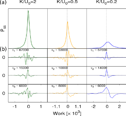
Figure 5: (a) Steady state probability distribution of work for the three regimes. In this case we applied a running average to the data, both for the steady–state distribution and the corrections. (b) The perturbations $g_{i}$ (see Eq. 4) estimated for the first three excited states. The observable $O$ in Eq. 4 is here the work. To compute $P(O|\alpha)$ 100 intervals have been chosen.

VI Conclusions

The Markov State Model method, so far developed for the equilibrium evolution of large–scale molecular systems, can be naturally extended to non-equilibrium dynamics under the action of external forces. Among non–equilibrium phenomena, the physics of sliding friction is in bad need of a description, with coarse–grained variables and their time evolution constructed in the least prejudiced manner. We have shown here that application of this technique to a realistic model involving a mesoscopically large sliding system is possible and fruitful.

Three important conclusions that were not a priori granted deserve being underlined. The first is that no particularly clever or savvy choice of the metric is necessary: the very naive choice of considering the distance between all the particles of the sliding island works very well. Since the metric is so simple, the kinetic model that is obtained is likely to be accurate. The second, and equally remarkable result is that despite many thousands of atomistic degrees of freedom, the procedure allows selecting just very few slow variables, automatically eliminating all other fast irrelevant variables. The third is that the slow variables, once examined at the end, are found to make a lot of sense when confronted with the actual frictional physics of the system, be it superlubric or stick–slip. These gratifying bottomlines provide a strong encouragement towards the future use of the MSM for the theoretical description of sliding friction.

References

- Vanossi et al. (2013) A. Vanossi, N. Manini, M. Urbakh, S. Zapperi, and E. Tosatti, Reviews of Modern Physics 85, 529 (2013).
- Pellegrini et al. (2016) F. Pellegrini, F.P. Landes, A. Laio, S. Prestipino, and E. Tosatti, Physical Review E 94, 053001 (2016).
- Noé et al. (2009) F. Noé, C. Schütte, E. Vanden-Eijnden, L. Reich, and T. R. Weikl, Proceedings of the National Academy of Sciences of the United States of America 106, 19011 (2009).
- Schwantes et al. (2014) C. R. Schwantes, R. T. McGibbon, and V. S. Pande, The Journal of Chemical Physics 141, 090901 (2014).
- Noé and Nüske (2013) F. Noé and F. Nüske, Multiscale Modeling & Simulation 11, 635 (2013).
- Bowman et al. (2014) G. R. Bowman, V. S. Pande, and F. Noé, in An Introduction to Markov State Models and Their Application to Long Timescale Molecular Simulation, Springer (2014).
- Schütte and Sarich (2015) C. Schütte and M. Sarich, The European Physical Journal Special Topics 18 (2015).
- Frenkel and T.A. Kontorova (1938) Y. I. Frenkel and T. A. Kontorova, Phys. Z. Sowietunion 13 (1938).
- Pérez-Hernández et al. (2013) G. Pérez-Hernández, F. Paul, T. Giorgino, G. De Fabritiis, and F. Noé, The Journal of Chemical Physics 139, 015102 (2013).
- Deuflhard and Weber (2005) P. Deuflhard and M. Weber, Linear Algebra and its Applications 398, 161 (2005).
- Weber and Kube (2005) M. Weber and S. Kube, Lecture Notes in Computer Science 3695, 57 (2005).
- Prinz et al. (2011) J.-H. Prinz, H. Wu, M. Sarich, B. Keller, M. Senne, M. Held, J. D. Chodera, C. Schütte, and F. Noé, The Journal of Chemical Physics 134, 174105 (2011).
- Rodriguez and Laio (2014) A. Rodriguez and A. Laio, Science 344, 1492 (2014).
- Braun and Kivshar (1998) O. M. Braun and Y. S. Kivshar, Physics Reports 306, 1 (1998).
- Varini et al. (2015) N. Varini, A. Vanossi, R. Guerra, D. Mandelli, R. Capozza, and E. Tosatti, Nanoscale 7, 2093 (2015).
- (16) C. Schütte, F. Noé, J. Lu, M. Sarich, and E. Vanden-Eijnden, The Journal of Chemical Physics 134, 204105 (2011).