Quantum correlations between distant qubits conveyed by large-$S$ spin chains

Abstract

We consider two distant spin-$\frac{1}{2}$ particles (or qubits) and a number of interacting objects, all with the same value $S\gg 1$ of their respective spin, distributed on a one-dimensional lattice (or large-$S$ spin chain). The quantum states of the chain are constructed by linearly combining tensor products of single-spin coherent states, whose evolution is determined accordingly, i.e., via classical-like equations of motions. We show that the quantum superposition of the above product states resulting from a local interaction between the first qubit and one spin of the chain evolves so that the second qubit, after having itself interacted with another spin of the chain, can be entangled with the first qubit. Obtaining such outcome does not imply imposing constraints on the length of the chain or the distance between the qubits, which demonstrates the possibility of generating quantum correlations at a distance by means of a macroscopic system, as far as local interactions with just a few of its components are feasible.

I Introduction

Whenever dealing with quantum devices one needs to accommodate antithetical requirements: On the one hand, microscopic objects must be isolated from their environment to protect the quantum behavior which is key to the device functioning. On the other hand, they need communicating with the external world in order to accomplish some useful task. This suggests that a hybrid scheme might be necessary in order to meet both requirements, where by hybrid we mean a system where the fragile quantum component (one or more qubits) is accompanied by a robust, almost classical partner, which mediates the dialog between each qubit and the external world without significantly exposing it, but still being able of conveying quantum correlations.

Specifically addressing the case of quantum operations such as state transfer or entanglement generation, the most promising proposals are typically based on the use of quantum channels made of interacting qubits  Bose2003 ; CamposVenutiEtal2007 ; BanchiEtal2011 ; CampbellEtAl2011 ; ApollaroBCVV2012 ; PaganelliEtAl2013 ; Kay2010 ; KarbachS2005 ; ChristandlDEL2004 ; YungB2005 ; DiFrancoPK2008 ; AhmedG2015 ; ZwickASO2011 ; WangSR2011 , whose expected high performances entail a high sensitivity to decoherence, raising the necessity of protection from external disturbances. This level of protection could be alleviated if it were possible to exploit the more robust dynamical features of a system made by interacting objects with a large value of their spin angular momentum, $S\gg 1$, possibly arranged on a one-dimensional (1D) lattice, so as to make up the system that we will hereafter call ”large-$S$ spin chain”. Indeed, a classical analysis based on the $S\to\infty$ limit, has recently shown that such a spin chain can be made to evolve in a way such that robust signals (specifically magnetic solitons) are transmitted along macroscopic distances, giving rise to an overall dynamics that fulfills single-qubit state manipulation CNVV2014a ; CNVV2015a . However, in order to demonstrate that a large-$S$ spin-chain can also be used for generating entanglement between distant qubits, a quantum treatment of its dynamics must be considered.

The exact quantum description of large-$S$ spin chains of sizeable length is usually unattainable, even numerically, due to their huge Hilbert space and the specific algebra obeyed by the spin operators: therefore, ad hoc methods must be devised to deal with such a problem. Generalized Coherent States (GCS) Perelomov1986 ; ZhangFG1990 provide a powerful tool for describing the dynamics of quantum systems in this context CalvaniCGV2013 ; BalakrishnanB1989 ; DiosiS1997 ; HelmSRW2011 ; Combescure1992 , as they keep a clear correspondence between the quantum picture and the increasingly classical behavior observed when the system quanticity parameter (e.g., $1/S$ for spins) tends to zero Lieb73 ; Yaffe82 .

Aim of this work is to illustrate the possibility of generating entanglement between two qubits separated by a macroscopic distance by means of their interaction with localized components of a large-$S$ spin chain. This is made possible by treating such a hybrid system within an approximate description, based on the properties of GCS for the large-$S$ spin chain, that retains enough of the spin-chain quantum nature to account for quantum correlations. Specifically, we choose an isotropic Heisenberg chain, referred to as $\Gamma$ henceforth, composed by elementary objects with spin quantum number $S$ larger than $1/2$, and two external qubits ${\rm{A}}$ and ${\rm{B}}$ interacting with two spins ${\bm{S}}_{{\rm{A}}}$ and ${\bm{S}}_{{\rm{B}}}$ of the chain, as shown in Fig. 1. Starting from a factorized state of the chain and the two qubits, we study whether the entanglement locally created by the interaction between ${\rm{A}}$ and ${\bm{S}}_{{\rm{A}}}$ can propagate along the chain up to ${\bm{S}}_{{\rm{B}}}$ and be finally transferred to ${\rm{B}}$, the net result being the generation of entanglement between ${\bm{S}}_{{\rm{A}}}$ and ${\bm{S}}_{{\rm{B}}}$ .

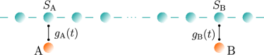
Figure 1: Schematic representation of the system: the connected blue spheres represent the spins of a Heisenberg chain, while the orange ones are the two qubits.

The initial state of $\Gamma$ is taken as a tensor product of single-spin coherent states (SCS), which allows us to establish a one-to-one correspondence between the configurations of a classical spin chain and the quantum states of $\Gamma$. Indeed, if $\Gamma$ sustains the propagation of Heisenberg solitons TjonW1977 ; Takhtajan1977 (i.e., well-localized, stable, pulse-shaped excitations), their propagation can trigger the interaction with the two qubits and convey the quantum correlations between them.

In Sec. II we describe the model for the overall system and specify the interactions between its components. The system dynamics is then divided into three different stages, which are considered in Secs. III, V, and VI. Role of Sec. IV is that of providing a formal derivation of the GCS for the large-$S$ Heisenberg chain, while Sec. VII is devoted to the discussion of our numerical results and the concluding remarks.

II Model set-up

The Hamiltonian describing the overall system is taken of the form:

$${\cal H}={\cal H}_{{\rm{A}}{,}{\bm{S}}_{{\rm{A}}}}+{\cal H}_{\Gamma}+{\cal H}_{{\rm{B}}{,}{\bm{S}}_{{\rm{B}}}},$$ (1)

where

$${\cal H}_{{\rm{A}}{,}{\bm{S}}_{{\rm{A}}}}=g_{{\rm{A}}}\,\hat{\bm{S}}_{{\rm{A}}}{\cdot}\,\hat{\bm{\sigma}}_{{\rm{A}}}+h_{{\rm{A}}}\hat{\sigma}_{{\rm{A}}}^{z}~{},$$ (2)

and similarly for ${\cal H}_{{\rm{B}}{,}{\bm{S}}_{{\rm{B}}}}$, with ${\rm{A}}\leftrightarrow{\rm{B}}$; $\hat{\bm{\sigma}}_{{\rm{A}}}$ and $\hat{\bm{\sigma}}_{{\rm{B}}}$ are the Pauli operators of the qubits, whose interaction with ${\bm{S}}_{{\rm{A}}}$ and ${\bm{S}}_{{\rm{B}}}$ is ruled by the coupling constants $g_{{\rm{A}}}$ and $g_{{\rm{B}}}$, while $h_{{\rm{A}}}$ and $h_{{\rm{B}}}$ are uniform magnetic fields possibly applied to the qubits only. The Hamiltonian of the chain

$${\cal H}_{\Gamma}=-J\sum_{n}\hat{\bm{S}}_{n}{\cdot}\hat{\bm{S}}_{n+1}-\gamma H\sum_{n}\hat{S}_{n}^{z}$$ (3)

embodies a nearest-neighbor isotropic ferromagnetic interaction, whose strength is given by the exchange constant $J>0$, and that with an external field ${\bm{H}}$, $\gamma$ being the gyromagnetic ratio; amongst the possible solutions of the equations of motions defined by ${\cal H}_{\Gamma}$ in the $S\to\infty$ and continuum limit, for $H\neq 0$ there are the so-called Heisenberg solitons TjonW1977 ; in Appendix A we briefly recall the properties of such solutions that are relevant in this work.

We further assume that the qubit-chain couplings $g_{{\rm{A}}}$ and $g_{{\rm{B}}}$ depend on time, and are switched on and off according to

$$g_{{\rm{A}}}(t)=g\,\vartheta(t{-}t_{0})\,\vartheta(t_{1}{-}t)~{},$$ (4)

$$g_{{\rm{B}}}(t)=g\,\vartheta(t{-}t_{2})\,\vartheta(t_{3}{-}t)~{},$$

with $\vartheta(t)$ the Heaviside function, and $g$ the interaction strength. By Eqs. (4) the overall evolution is decomposed into three stages, and $g$ sets the time-scale for the first and third ones.

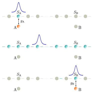
Figure 2: Schematic representation of the three stages of the system dynamics (1), (2) and (3) from top to bottom, respectively (see text).

In more detail, assuming an initial factorized state, the system evolution from $t_{0}$ to $t_{3}$ (see Fig. 2 for a graphic representation) is described as follows:

• $[t_{0},t_{1}]$: $g_{{\rm{A}}}(t)=g$ and $g_{{\rm{B}}}(t)=0$. Starting from the factorized initial state the evolution of $({\rm{A}},{\bm{S}}_{{\rm{A}}})$ is determined. During this stage $\Gamma\setminus{\bm{S}}_{{\rm{A}}}$ is frozen, i.e., the spins $\{{\bm{S}}_{n}\}$ except ${\bm{S}}_{{\rm{A}}}$ note1 do not evolve. This leads to an entangled state of ${\rm{A}}$ and ${\bm{S}}_{{\rm{A}}}$.

• $[t_{1},t_{2}]$: $g_{{\rm{A}}}(t)=g_{{\rm{B}}}(t)=0$. The large-$S$ evolution of $\Gamma$ results in an entangled state of ${\rm{A}}$ with the entire chain.

• $[t_{2},t_{3}]$: $g_{{\rm{B}}}(t)=g$ and $g_{{\rm{A}}}(t)=0$. The relevant evolution only concerns the $({\rm{B}},{\bm{S}}_{{\rm{B}}})$ pair, and $\Gamma\setminus{\bm{S}}_{{\rm{B}}}$ is frozen. The eventual result is an entangled state of the whole system, with a finite concurrence between ${\rm{A}}$ and ${\rm{B}}$.

As for the dynamics of the system for $t<t_{0}$, the qubits and the spins in a portion of $\Gamma$ having ${\bm{S}}_{{\rm{A}}}$ and ${\bm{S}}_{{\rm{B}}}$ well within its bulk, stay all aligned along the field direction; meanwhile, a Heisenberg soliton travels from the left towards the above chain portion, so as to reach ${\bm{S}}_{{\rm{A}}}$ at $t=t_{0}$.

III First stage: evolution of $(A,{\bm{S}}_{{\rm{A}}})$

In the first stage we observe the evolution of the qubit ${\rm{A}}$ interacting with the spin ${\bm{S}}_{{\rm{A}}}$, while all the other spins of $\Gamma$ are frozen. The initial state at $t=t_{0}$ is assumed to be

$$|{\Psi(t_{0})}\rangle=|{A}\rangle\otimes\left[\,\bigotimes_{n}\big{|}{\Omega_{n}(t_{0})}\big{\rangle}\right]\otimes|{B}\rangle~{},$$ (5)

where $|{A}\rangle$ and $|{B}\rangle$ are the qubit states. The state of $\Gamma$, in brackets in Eq. (5), is a tensor product of single spin states, which are chosen as SCS Radcliffe1971 . The SCS form an overcomplete set on each Hilbert space $\mathscr{H}_{S_{n}}$ and they are in one-to-one correspondence with the configurations of a classical spin (namely a fixed-length vector), which implies that they can be parametrized by polar angles (see Appendix B). The main reason for the above choice of the chain initial state is that tensor products of SCS provide the GCS for the large-$S$ Heisenberg chain, as shown in the next section. In particular, the SCS that we will use in Eq. (5) are those defined by the polar angles corresponding to a Heisenberg-soliton shape, as described by Eq. (48) with $x=nd$. We further enforce the condition $n_{A}d=vt_{0}$, where ${\bm{S}}_{n_{A}}={\bm{S}}_{{\rm{A}}}$, $d$ is the lattice spacing, and $v$ is the soliton velocity, so that the traveling soliton be centered at $n_{A}$ for $t=t_{0}$.

The evolution of the system during the time interval $[t_{0},t_{1}]$ is described by

$${\cal U}^{(1)}(t)={\cal U}_{{\rm{A}}{,}{\bm{S}}_{{\rm{A}}}}(t)\otimes\mathds{1}_{\Gamma\setminus{\bm{S}}_{{\rm{A}}}}\otimes{\cal U}_{{\rm{B}}}(t)~{},$$ (6)

where

$${\cal U}_{{\rm{A}}{,}{\bm{S}}_{{\rm{A}}}}(t)=\exp(-i\,{\cal H}_{{\rm{A}}{,}{\bm{S}}_{{\rm{A}}}}\,t)~{},$$ (7)

is the propagator for the subsystem (${\rm{A}}$,${\bm{S}}_{{\rm{A}}}$), with ${\cal H}_{{\rm{A}}{,}{\bm{S}}_{{\rm{A}}}}$ as in Eq. (2), while

$${\cal U}_{{\rm{B}}}(t)=\exp(-i\,h_{{\rm{B}}}\hat{\sigma}_{{\rm{B}}}^{z}\,\,t)\,$$ (8)

accounts for the effect on ${\rm{B}}$ of the local field $h_{{\rm{B}}}$.

As far as $\Gamma\setminus{{\bm{S}}_{{\rm{A}}}}$ and ${\rm{B}}$ are concerned, the action of ${\cal U}^{(1)}(t{-}t_{0})$ on the state (5) is trivial; however, the subsystem $({\rm{A}},{\bm{S}}_{{\rm{A}}})$ can evolve into an entangled state, as shown in Fig. 3, where the Von Neumann entropy $E_{{{\rm{A}},{\bm{S}}_{{\rm{A}}}}}(\big{|}{\psi_{{\rm{A}},{\bm{S}}_{{\rm{A}}}}(t)}\big{\rangle})$ of ${\rm{A}}$ is shown as a function of time note2 , for one initial state of ${\bm{S}}_{{\rm{A}}}$ and ${\rm{A}}$ and given values of the relevant parameters (times and lengths in figures are in reduced units of $(JS)^{-1}$ and $d$, respectively).

As we aim at generating entanglement between ${\rm{A}}$ and ${\rm{B}}$ via $\Gamma$, we will choose $t_{1}$ so as to maximize the numerically evaluated entanglement between ${\rm{A}}$ and ${\bm{S}}_{{\rm{A}}}$ at the end of the first dynamical stage. We thus ensure that the initial separable state of $({\rm{A}},{\bm{S}}_{{\rm{A}}})$ defined by Eq. (5),

$$\big{|}{\psi_{{\rm{A}},{\bm{S}}_{{\rm{A}}}}(t_{0})}\big{\rangle}=|{A}\rangle\otimes|{\Omega_{n_{{\rm{A}}}}(t_{0})}\rangle~{},$$ (9)

will evolve note3 into an entangled state

$$\big{|}{\psi_{{\rm{A}},{\bm{S}}_{{\rm{A}}}}(t)}\big{\rangle}=\sum_{\sigma{m}}c_{\sigma{m}}(t)|{\sigma}\rangle\otimes|{m}\rangle~{},$$ (10)

where $\{|{\sigma}\rangle\}$ and $\{|{m}\rangle\}$ are orthonormal basis for $\mathscr{H}_{A}$ and $\mathscr{H}_{{\bm{S}}_{{\rm{A}}}}$, respectively. By the completeness relation (55), the state at time $t_{1}$ can be written as

$$\big{|}{\psi_{{\rm{A}}{,}{\bm{S}}_{{\rm{A}}}}(t_{1})}\big{\rangle}=(2S{+}1)\sum_{\sigma}\int\frac{d\Omega}{4\pi}~{}f_{\sigma}^{\Omega}~{}|{\sigma}\rangle\otimes|{\Omega}\rangle~{},$$ (11)

with

$$f_{\sigma}^{\Omega}=\sum_{m}c_{\sigma{m}}(t_{1})~{}\langle{\Omega}|{m}\rangle~{},$$ (12)

and the overlap $\langle{\Omega}|{m}\rangle$ as in Eq. (51).

The evolved state of the overall system at the end of the first stage in the density-operator formalism reads

$$\big{|}{\Psi(t_{1})}\big{\rangle}\big{\langle}{\Psi(t_{1})}\big{|}=\big{|}{\psi_{{\rm{A}},{\bm{S}}_{{\rm{A}}}}(t_{1})}\big{\rangle}\big{\langle}{\psi_{{\rm{A}},{\bm{S}}_{{\rm{A}}}}(t_{1})}\big{|}\otimes$$

$$~{}~{}~{}~{}~{}~{}~{}\bigg{[}\bigotimes_{n\neq n_{{\rm{A}}}}\big{|}{\Omega_{n}(t_{0})}\big{\rangle}\big{\langle}{\Omega_{n}(t_{0})}\big{|}\bigg{]}\otimes\big{|}{B(t_{1})}\big{\rangle}\big{\langle}{B(t_{1})}\big{|}\,,$$ (13)

where $\big{|}{B(t_{1})}\big{\rangle}={\cal U}_{{\rm{B}}}(t_{1}-t_{0})|{B}\rangle$, and the term in brackets is the state of $\Gamma\setminus{\bm{S}}_{{\rm{A}}}$, that is left unchanged by the first-stage dynamics.

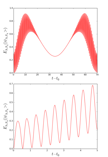
Figure 3: $E_{{{\rm{A}},{\bm{S}}_{{\rm{A}}}}}(t)$ for $t\in[t_{0},t_{1}]$, $S=5$, $g_{{\rm{A}}}=1$, $h_{{\rm{A}}}=0.25$. The ${\rm{A}}$ initial state is $|{1}\rangle$ while the chain is initially in the state corresponding to a propagating Heisenberg soliton (see text) with $\lambda_{\beta}=10$ and $\beta=\pi/4$ centered in $n_{A}$ (specifically meaning $\Omega^{0}_{n_{{\rm{A}}}}=\{\theta^{0}_{n_{{\rm{A}}}}=\pi/2,\varphi^{0}_{n_{{\rm{A}}}}=0\}$). The lower panel shows a zoom of the small-time part of the upper one.

IV Coherent states of the large-$S$ spin chain

This section contains a formal derivation of GCS for the Heisenberg spin chain with $S\gg{1}$. It will be shown that in the large-$S$ limit the GCS become a tensor product of SCS, as defined in Eq. (49), thus leading to the approximate evolution that is described in the next section.

The construction of the GCS ZhangFG1990 for a quantum system of Hamiltonian $\cal{H}$ starts from writing

$${\cal H}=\sum_{i}b_{i}\hat{T}_{i}+{\rm h.c.}\,,$$ (14)

so as to identify the Lie algebra spanned by the operators $\big{\{}\hat{T}_{i}\big{\}}$; the transformation group obtained by exponentiating the elements of such algebra is the so-called dynamical group (DG), i.e., the unitary group ruling the dynamics of the system.

Keeping in mind that we aim at considering a large-$S$ spin chain, we recast ${\cal H}_{\Gamma}$ in a form that fits to the purpose. First, since the energy has to stay finite, we notice that the exchange constant and the gyromagnetic ratio must scale with $S$ so as to guarantee that $J_{\rm{c}}\equiv JS^{2}$ and $\gamma_{\rm{c}}\equiv\gamma{S}$ have fixed, finite, values. We then define the operators

$$\hat{a}_{n}\equiv\frac{\hat{S}^{x}_{n}+i\hat{S}^{y}_{n}}{\sqrt{2}\,S}~{},~{}~{}~{}~{}\hat{z}_{n}\equiv\frac{\hat{S}^{z}_{n}}{S}$$ (15)

that satisfy $[\hat{a}_{n},\hat{a}^{\dagger}_{n}]=S^{-1}\hat{z}_{n}$ and $[\hat{z}_{n},\hat{a}_{n}]=S^{-1}\hat{a}_{n}$, in terms of which it is

$$\frac{{\cal H}_{\Gamma}}{J_{\rm{c}}}=-\sum_{n=1}^{N}\big{(}\hat{a}^{\dagger}_{n}\hat{a}_{n+1}+\hat{a}^{\dagger}_{n+1}\hat{a}_{n}+\hat{z}_{n}\hat{z}_{n+1}+h\hat{z}_{n}\big{)},$$ (16)

where $h=\gamma_{\rm{c}}H/J_{\rm{c}}$, and, for the sake of simplicity, periodic boundary conditions are assumed. Now we must find a set of operators that contains the $6N$ operators

$$\big{\{}\hat{a}^{\dagger}_{n},\,\hat{a}_{n},\,\hat{z}_{n},\,\hat{a}^{\dagger}_{n}\hat{a}_{n\pm 1},\,\hat{z}_{n}\hat{z}_{n+1}\big{\}}~{}$$ (17)

and is closed with respect to commutation; the ‘first generation’ of commutators, namely those between the above operators, yields $4N$ new bilinear operators, namely

$$\Big{\{}\frac{\hat{a}^{\dagger}_{n}\hat{z}_{n\pm 1}}{S},\,\frac{\hat{a}_{n}\hat{z}_{n\pm 1}}{S}\Big{\}},$$ (18)

as well as $10N$ new trilinear operators

$$\Big{\{}\frac{\hat{z}_{n}\hat{a}^{\dagger}_{r}\hat{a}_{s}}{S}\Big{\}}~{},$$ (19)

where $(n,r,s)$ is either a permutation of three consecutive numbers, or $(r,s)=(n,n\pm 1)$, or $(r,s)=(n\pm 1,n)$.

It is clear that the exact Lie algebra won’t have a finite number of generators, since subsequent generations of order $k$ give rise to new independent operators with prefactor $S^{-k}$, such as $S^{-2}\hat{a}_{n}\hat{a}_{n\pm 1}$. This is the reason why an exact construction of the GCS for the Heisenberg chain is not possible. However, for large $S$ one can disregard higher generations (i.e., approximate $S^{-2}\simeq{0}$) and close the Lie algebra with the above operators (17-19).

Once the Lie Algebra that generate the DG is determined, the GCS are obtained by the action of displacement operators on an arbitrary reference state; given the physical problem we are dealing with, this can be chosen as the ground state of the Hamiltonian (3), i.e.,

$$\big{|}{\Lambda}\big{\rangle}\,\equiv\,\bigotimes_{n}\big{|}{m_{n}{=}S}\big{\rangle}_{n}\,,$$ (20)

where $\hat{S}_{n}^{z}\,|{m_{n}}\rangle_{n}=m_{n}\,|{m_{n}}\rangle_{n}$, so that $\hat{z}_{n}\,|{\Lambda}\rangle=\,|{\Lambda}\rangle$.

The displacement operators are the elements of the left coset of the DG with respect to the so-called stability subgroup, which is the maximal subgroup of the DG that leaves the reference state unchanged up to a constant phase-factor. In our case the stability subgroup is generated by

$$\Big{\{}\hat{z}_{n},~{}\hat{z}_{n}\hat{z}_{n+1},~{}\hat{a}^{\dagger}_{n}\hat{a}_{n\pm 1},\,\frac{\hat{z}_{n}\hat{a}^{\dagger}_{r}\hat{a}_{s}}{S}\Big{\}}\,,$$ (21)

since $\big{|}{\Lambda}\big{\rangle}$ either is an eigenstate of these operators, or is annihilated by them. By definition, the left-coset representatives are given by those elements $\tilde{u}$ providing a unique decomposition of any $u\in$ DG in the form

$$u=\tilde{u}\,u^{\prime}\,,$$ (22)

where $u^{\prime}$ belongs to the stability subgroup. Within the large-$S$ approximation, it appears that the general representative of the left coset of the stability subgroup is given by

$$\tilde{u}=\exp\Big{[}\,\sum_{n=1}^{N}\Big{(}\eta_{n}+\zeta^{+}_{n}\frac{\hat{z}_{n+1}}{S}+\zeta^{-}_{n}\frac{\hat{z}_{n-1}}{S}\Big{)}\hat{a}^{\dagger}_{n}-{\rm h.c.}\Big{]}~{},$$ (23)

where $\eta\equiv(\eta_{1},\ldots,\eta_{N})$, $\zeta^{\pm}\equiv(\zeta^{\pm}_{1},\ldots,\zeta^{\pm}_{N})$ are complex vectors. Since the operators in the exponent of the above expression commute in the large-$S$ approximation, one can write the displacement operator as a product of exponentials, and recast Eq. (23) as

$$\tilde{u}=\bigotimes_{n=1}^{N}\exp\Big{[}\Big{(}\eta_{n}+\zeta^{+}_{n}\frac{\hat{z}_{n+1}}{S}+\zeta^{-}_{n}\frac{\hat{z}_{n-1}}{S}\Big{)}\hat{a}^{\dagger}_{n}-{\rm h.c.}\Big{]}~{}.$$ (24)

By applying this operator to the chosen reference state (20) one obtains

$$\tilde{u}\,\big{|}{\Lambda}\big{\rangle}=\bigotimes_{n}\Big{[}e^{\xi_{n}\hat{a}^{\dagger}_{n}-\xi^{*}_{n}\hat{a}_{n}}\,|{m_{n}{=}S}\rangle_{n}\Big{]}~{},$$ (25)

with $\xi_{n}=\eta_{n}{+}(\zeta_{n}^{+}{+}\zeta_{n}^{-})/S$.

Setting $\xi_{n}=(\sqrt{2}S)^{-1}e^{i\varphi}(\theta/2)$, a one-to-one correspondence is established between the states that make the tensor product in Eq. (25) and the SCS defined in Eq. (49), after recognition of the parameters $\theta$ and $\varphi$ as the polar angles entering the latter. This correspondence implies that the GCS for the spin chain in the large-$S$ limit, hereafter indicated by $|{\Omega_{\Gamma}}\rangle$, are a tensor product of SCS, each relative to one spin of the chain, i.e.

$$|{\Omega_{\Gamma}}\rangle\equiv\tilde{u}|{\Lambda}\rangle=\bigotimes_{n}|{\Omega_{n}}\rangle;$$ (26)

this result, together with the observation that the dynamical properties of one-dimensional magnetic systems with large $S$ are well represented by classical equations of motion (EoM), leads to describe the chain evolution as in the next section.

V Second stage: evolution of the chain

When the second stage begins, at $t=t_{1}$, the interaction $g_{{\rm{A}}}(t)$ with ${\rm{A}}$ is quenched and the overall propagator for $t\in[t_{1},t_{2}]$ can be split as

$${\cal U}^{(2)}(t)={\cal U}_{{\rm{A}}}(t)\otimes{\cal U}_{\Gamma}(t)\otimes{\cal U}_{{\rm{B}}}(t)\,,$$ (27)

where ${\cal U}_{{\rm{A}}}(t)$ is the operator on ${\rm{A}}$ analogous to that in Eq. (8), while ${\cal U}_{\Gamma}(t)$ is the chain propagator.

After the results of the previous section, we consistently take that the dynamics of each $|{\Omega_{n}}\rangle$ be given by the solution of the classical-like EoM for the chain, meaning that any initial state $|{\Omega^{0}_{\Gamma}}\rangle=\bigotimes_{n}|{\Omega^{0}_{n}}\rangle$ evolves following the dynamics of the associated classical configuration, $\{{\bm{S}}_{n}(t)=S\,{\bm{s}}_{n}(t)\}$ as from Eq. (52), with ${\bm{s}}_{n}(t)$ solving the classical EoM, Eqs. (47), i.e.

$$\begin{array}[]{@{}cl@{\quad}@{}c@{\quad}@{}c}\big{\{}\Omega^{0}_{n}\big{\}}&\xrightarrow[]{\text{~{}classical~{}EoM~{}(A2)~{}}}&\big{\{}\Omega_{n}\big{(}t;\{\Omega^{0}_{n}\}\big{)}\big{\}}~{},{}{}\\[5.69054pt] \bigotimes_{n}|{\Omega^{0}_{n}}\rangle&\xrightarrow[]{\text{~{}~{}~{}~{}~{}~{}~{}large-}S~{}~{}~{}~{}~{}~{}~{}}&\bigotimes_{n}\big{|}{\Omega_{n}\big{(}t,\{\Omega^{0}_{n}\}\big{)}}\big{\rangle}~{}.\end{array}$$ (28)

This prescription provides a dynamics that reproduces the correct evolution of the spin expectation values in the classical limit, and still maintains the quantum character of $\Gamma$, allowing the entanglement between ${\rm{A}}$ and ${\bm{S}}_{{\rm{A}}}$, generated during the first stage of the scheme, to be transferred via the spins of the chain. In fact, if one starts from a pure state of $\Gamma$ which is factorized in the SCS basis, the above evolution cannot transfer quantum correlations, being based on the dynamics of separable SCS. However, the state of $\Gamma$ when the second stage begins is not pure, due to ${\bm{S}}_{{\rm{A}}}$ being entangled with $A$, as implied by Eq. (11). Explicitly, once applied to the initial state Eq. (13), i.e. to

$$\big{|}{\psi_{{\rm{A}},\Gamma}(t_{1})}\big{\rangle}=\big{|}{\psi_{{\rm{A}},{\bm{S}}_{{\rm{A}}}}(t_{1})}\big{\rangle}\bigotimes_{n\neq n_{{\rm{A}}}}|{\Omega_{n}(t_{0})}\rangle~{},$$ (29)

with $\big{|}{\psi_{{\rm{A}},{\bm{S}}_{{\rm{A}}}}(t_{1})}\big{\rangle}$ as in Eq.(11), the above prescription (28) leads, during the second stage, to the projector

$$\big{|}{\Psi(t)}\big{\rangle}\!\big{\langle}{\Psi(t)}\big{|}=\big{|}{\psi_{{\rm{A}},\Gamma}(t)}\big{\rangle}\!\big{\langle}{\psi_{{\rm{A}},\Gamma}(t)}\big{|}\otimes\big{|}{B(t)}\big{\rangle}\!\big{\langle}{B(t)}\big{|}~{},$$ (30)

with $|{B(t)}\rangle={\cal U}_{{{\rm{B}}}}(t)|{B}\rangle$ and

$$\big{|}{\psi_{{\rm{A}},\Gamma}(t)}\big{\rangle}={\cal{A}}\sum_{\sigma}\int d\Omega~{}f_{\sigma}^{\Omega}\big{|}{\sigma(t)}\big{\rangle}\bigotimes_{n}\big{|}{\Omega_{n}(t,\Omega)}\big{\rangle}\,,$$ (31)

where $|{\sigma(t)}\rangle={\cal U}_{{\rm{A}}}(t-t_{1})|{\sigma}\rangle$, ${\cal{A}}$ is a normalization coefficient, and we have dropped the unimportant dependence of $\Omega_{n}(t)$ on all the $\{\Omega^{0}_{n}\equiv\Omega_{n}(t_{0})\}$ with $n\neq n_{A}$, retaining only the meaningful dependence on $\Omega\equiv\Omega^{0}_{n_{A}}$.

In order to identify when it is worth starting the third stage of the dynamical process, i.e. what is the best choice for $t_{2}$ as far as the further entanglement generation between A and B is concerned, we consider what follows. Given the Hamiltonian (1), the qubit ${\rm{B}}$ can become entangled with other components of the system, including ${\rm{A}}$, exclusively via the interaction with ${\bm{S}}_{{\rm{B}}}$: entanglement generation between the two qubits can hence occur only if ${\bm{S}}_{{\rm{B}}}$ is entangled with $({\rm{A}},\Gamma\setminus{\bm{S}}_{{\rm{B}}})$ at $t=t_{2}$, and we expect its effectiveness to be higher if $t_{2}$ is such to guarantee a significant entanglement between ${\rm{A}}$ and ${\bm{S}}_{{\rm{B}}}$ at the beginning of the third stage. Establishing when this is the case implies determining the time-dependence of the Von Neumann entropy $E_{{{\bm{S}}_{n}}}$ of any spin ${\bm{S}}_{n}$ of the chain, that quantifies the entanglement between ${\bm{S}}_{n}$ and $({\rm{A}},\Gamma\setminus{\bm{S}}_{n})$. This entropy reads

$$E_{{{\bm{S}}_{n}}}=-\operatorname{Tr}_{{}_{{\bm{S}}_{n}}}\rho_{{}_{{\bm{S}}_{n}}}\log_{2S{+}1}\rho_{{}_{{\bm{S}}_{n}}}~{},$$ (32)

where

$$\rho_{{}_{{\bm{S}}_{n}}}=\operatorname{Tr}_{({\rm{A}}{,}\Gamma)\setminus{\bm{S}}_{n}}\big{|}{\psi_{{\rm{A}},\Gamma}(t)}\big{\rangle}\big{\langle}{\psi_{{\rm{A}},\Gamma}(t)}\big{|}~{}.$$ (33)

Noticing that

$$\operatorname{Tr}_{{}_{{\bm{S}}_{l}}}\big{|}{\Omega_{l}(t,\Omega)}\big{\rangle}\langle{\Omega_{l}(t,\Omega^{\prime})}|=\big{\langle}{\Omega_{l}(t,\Omega^{\prime})}\big{|}{\Omega_{l}(t,\Omega)}\big{\rangle}~{},$$ (34)

we find, setting $f_{\sigma\sigma^{\prime}}^{\Omega\Omega^{\prime}}\equiv f_{\sigma}^{\Omega}f_{\sigma^{\prime}}^{\Omega^{\prime\displaystyle*}}$,

$$\rho_{{}_{{\bm{S}}_{n}}}(t)={\cal A}^{2}\operatorname{Tr}_{{}_{\rm{A}}}\sum_{\sigma\sigma^{\prime}}\int d\Omega d\Omega^{\prime}\,f_{\sigma\sigma^{\prime}}^{\Omega\Omega^{\prime}}\,\big{|}{\sigma(t)}\big{\rangle}\big{\langle}{\sigma^{\prime}(t)}\big{|}$$

$$~{}~{}~{}~{}~{}\times\bigg{[}\prod_{l\neq n}\big{\langle}{\Omega_{l}(t,\Omega^{\prime})}\big{|}{\Omega_{l}(t,\Omega)}\big{\rangle}\bigg{]}$$

$$~{}~{}~{}~{}~{}\otimes|{\Omega_{n}(t,\Omega)}\rangle\langle{\Omega_{n}(t,\Omega^{\prime})}|~{}.$$ (35)

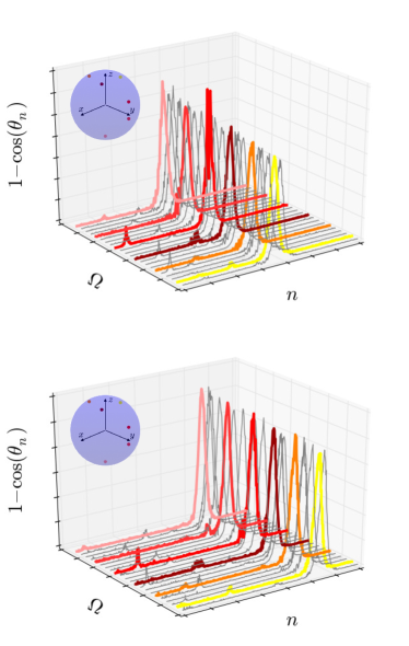
Figure 4: Configurations $\Omega_{n}(t,\Omega)$ for a starting soliton with $\lambda_{\beta}=10$, visualized via $(1-\cos\theta_{n}(t,\Omega))$ as functions of $n$ and $\Omega$, after an integration time $t-t_{1}$ equal to 400 (800) in the upper (lower) panel. Coloured curves are for $\Omega$’s that define correspondingly coloured points on the small sphere in the upper-left corner.

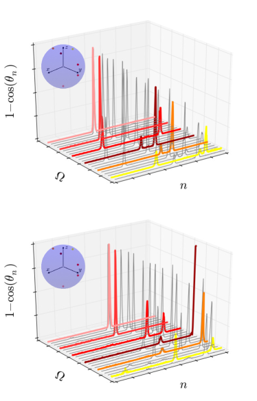
Figure 5: Same as in Fig. 4, for a starting soliton with $\lambda_{\beta}=2.5$ and integration times equal to 200 (upper panel) and 400 (lower panel).

Let us now concentrate upon the overlaps $\big{\langle}{\Omega_{l}(t,\Omega^{\prime})}\big{|}{\Omega_{l}(t,\Omega)}\big{\rangle}$ entering the above expression: if, for given $l$ and $t$, $\Omega_{l}(t,\Omega)$, only weakly depends on the initial value $\Omega$, the corresponding overlap is equal to one, the index $l$ disappears from Eq. (35), and the spin ${\bm{S}}_{l}$ effectively exits the dynamical scene. If this is the case for all but a small number of adjacent spins of the chain, the entanglement originally generated by the interaction of ${\rm{A}}$ with ${\bm{S}}_{{\rm{A}}}$ is not spread along the whole chain, but remains confined to the portion made of the above adjacent spins, whose configurations substantially depend on the initial value $\Omega$.

In fact, this is precisely what happens in our setting when the initial configuration of the chain corresponds to a Heisenberg soliton whose width is larger than the chain spacing, as seen by comparing Figs. 4 and 5: while for $\lambda_{\beta}=2.5$ (Fig. 5) different $\Omega$ generate quite diverse configurations $\Omega_{n}(t,\Omega)$, if $\lambda_{\beta}=10$ (Fig. 4) the dependence of $\Omega_{n}(t,\Omega)$ on $\Omega$ is weaker and localized in a limited region of $\Gamma$. In this latter case, the soliton moves forward with a slightly modified shape and hauls the deformation of $\Omega_{n_{{\rm{A}}}}(t_{0})$ imposed while it traveled through site $n_{{\rm{A}}}$. We can hence expect that, during the second stage of our scheme, the soliton behave as a carrier that keeps the entanglement localized while traveling along the chain.

Numerical results do confirm this picture, as seen in Fig. 6, where snapshots of $E_{{{\bm{S}}_{n}}}$ are reported as a function of $n$. In the first panel of Fig. 6 a bump is clearly visible, centered at about $n=n_{A}+v(t-t_{1})$, with $v$ the soliton velocity, which means that only the spins around the soliton are significantly entangled with the rest of the system. The different curves report the same quantity for different values of $S$: the shape is almost unchanged, but the values monotonically decrease with increasing $S$, according to the fact that in the limit $S\to\infty$ the entanglement disappears as the spins become completely classical.

The most favorable condition to establish entanglement between ${\rm{A}}$ and ${\rm{B}}$ is therefore achieved by choosing the time $t_{2}$ when the soliton crosses $n_{{\rm{B}}}$: the superposition of the evolved configurations obtained from different deformations $\Omega$, Eq. (31), is indeed expected to concentrate at such time around $n_{{\rm{B}}}$ the entanglement collected at time $t_{1}$ in $n_{{\rm{A}}}$.

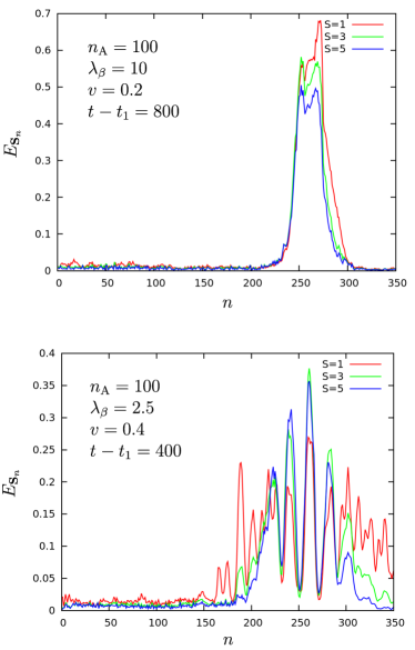
Figure 6: $E_{{{\bm{S}}_{n}}}(t)$ as a function of $n$ at $t-t_{1}=800$ with a starting soliton of width $\lambda_{\beta}=10$ (upper panel) and at $t-t_{1}=400$ with a starting soliton of width $\lambda_{\beta}=2.5$ (lower panel). Curves for different values of $S$, as indicated.

VI Third stage: evolution of $({\rm{B}},{\bm{S}}_{{\rm{B}}})$

During the third stage, ${\rm{A}}$ is only affected by a uniform field, $\Gamma\setminus{\bm{S}}_{{\rm{B}}}$ does not evolve, and ${\rm{B}}$ interacts with ${\bm{S}}_{{\rm{B}}}$ via the coupling $g_{{\rm{B}}}(t)=g$. Apart from the different initial state, this stage is analogous to the first one with ${\rm{A}}\leftrightarrow{\rm{B}}$: in fact, the propagator for $t\in[t_{2},t_{3}]$ is

$${\cal U}^{(3)}(t)={\cal U}_{{\rm{A}}}(t)\otimes\mathds{1}_{\Gamma\setminus{\bm{S}}_{{\rm{B}}}}\otimes{\cal U}_{{\rm{B}},{\bm{S}}_{{\rm{B}}}}(t)\,,$$ (36)

to be compared with Eq. (6). As we are interested in the entanglement between ${\rm{A}}$ and ${\rm{B}}$, we now have to determine the two-qubit density operator $\rho_{{\rm{A}}{\rm{B}}}(t)$. Performing the partial trace of the projector (30) upon $\Gamma\setminus{{\bm{S}}_{{\rm{B}}}}$ at $t=t_{2}$ we obtain the initial state for the third stage, i.e.

$$\rho_{{\rm{A}}{,}{\bm{S}}_{{\rm{B}}}{,}{\rm{B}}}(t_{2}) = \operatorname{Tr}_{\Gamma\setminus{{\bm{S}}_{{\rm{B}}}}}\big{|}{\Psi(t_{2})}\big{\rangle}\big{\langle}{\Psi(t_{2})}\big{|}$$ (37)

$$= \rho_{{\rm{A}}{,}{\bm{S}}_{{\rm{B}}}}(t_{2})\otimes\big{|}{B(t_{2})}\big{\rangle}\big{\langle}{B(t_{2})}\big{|}~{},$$ (38)

with

$$\rho_{{\rm{A}}{,}{\bm{S}}_{{\rm{B}}}}(t_{2})={\cal A}^{2}\sum_{\sigma\sigma^{\prime}}\int d\Omega d\Omega^{\prime}\,f_{\sigma\sigma^{\prime}}^{\Omega\Omega^{\prime}}\,\big{|}{\sigma(t_{2})}\big{\rangle}\big{\langle}{\sigma^{\prime}(t_{2})}\big{|}$$

$$~{}~{}~{}~{}~{}\times\bigg{[}\prod_{n\neq n_{{\rm{B}}}}\big{\langle}{\Omega_{n}(t_{2},\Omega^{\prime})}\big{|}{\Omega_{n}(t_{2},\Omega)}\big{\rangle}\bigg{]}$$

$$~{}~{}~{}~{}~{}\otimes|{\Omega_{\rm{B}}(t_{2},\Omega)}\rangle\langle{\Omega_{\rm{B}}(t_{2},\Omega^{\prime})}|~{},$$ (39)

where $\Omega_{\rm{B}}\equiv\Omega_{n_{{\rm{B}}}}$. Notice that, having traced out all the spins of $\Gamma$ but ${\bm{S}}_{{\rm{B}}}$, for $t>t_{2}$ we deal with the Hilbert space of ${\rm{A}},{\rm{B}}$ and ${\bm{S}}_{{\rm{B}}}$ only, which has dimension $4(2S{+}1)$ no matter the distance between the qubits, i.e. the length of the portion of chain between ${\bm{S}}_{{\rm{A}}}$ and ${\bm{S}}_{{\rm{B}}}$. The propagator for $({\rm{A}},{\bm{S}}_{{\rm{B}}},{\rm{B}})$ is $\exp\{-i{\cal H}_{{\rm{A}}{,}{\bm{S}}_{{\rm{B}}}{,}{\rm{B}}}\,t\}$, with

$${\cal H}_{{\rm{A}}{,}{\bm{S}}_{{\rm{B}}}{,}{\rm{B}}}=h_{{\rm{A}}}\hat{\sigma}_{{\rm{A}}}^{z}+g\,\hat{\bm{S}}_{{\rm{B}}}{\cdot}\,\hat{\bm{\sigma}}_{{\rm{B}}}+h_{{\rm{B}}}\hat{\sigma}_{{\rm{B}}}^{z}~{},$$ (40)

that can be diagonalized numerically note3 ; the generic element of the density matrix of $({\rm{A}},{\bm{S}}_{{\rm{B}}})$ can be written as

$$\big{[}\rho_{{{\rm{A}}{,}{\bm{S}}_{{\rm{B}}}}}(t_{2})\,\big{]}_{mm^{\prime}}^{\sigma\sigma^{\prime}}={\cal A}^{2}e^{-ih(t_{2}-t_{1})(\sigma{-}\sigma^{\prime})}\int d\Omega\,d\Omega^{\prime}\,f_{\sigma\sigma^{\prime}}^{\Omega\Omega^{\prime}}$$

$$~{}\times~{}\bigg{[}\prod_{n\neq n_{{\rm{B}}}}\big{\langle}{\Omega_{n}(t_{2},\Omega^{\prime})}\big{|}{\Omega_{n}(t_{2},\Omega)}\big{\rangle}\bigg{]}{\cal D}_{mm^{\prime}}^{\Omega\Omega^{\prime}}(t_{2})~{},$$ (41)

with

$${\cal D}_{mm^{\prime}}^{\Omega\Omega^{\prime}}(t_{2})=\big{\langle}{m}\big{|}{\Omega_{\rm{B}}(t_{2},\Omega)}\big{\rangle}\big{\langle}{\Omega_{\rm{B}}(t_{2},\Omega^{\prime})}\big{|}{m^{\prime}}\big{\rangle}\,.$$ (42)

Given Eqs. (38)–(41), making use of the relations (51) and (53) one can numerically compute $\rho_{{{\rm{A}}{,}{\bm{S}}_{{\rm{B}}}{,}{\rm{B}}}}(t_{2})$ and its evolved state with $t$ any time larger than $t_{2}$. Although $\rho_{{{\rm{A}}{,}{\bm{S}}_{{\rm{B}}}{,}{\rm{B}}}}(t)$ is in general a non-separable state of ${\rm{B}}$ and $({\rm{A}},{\bm{S}}_{{\rm{B}}})$, this does not necessarily mean that ${\rm{A}}$ and ${\rm{B}}$ are entangled. In order to settle this, one has to trace out ${\bm{S}}_{{\rm{B}}}$, yielding the two-qubit density operator

$$\rho_{{{\rm{A}}{,}{\rm{B}}}}(t)=\operatorname{Tr}_{{\bm{S}}_{{\rm{B}}}}\left[\rho_{{{\rm{A}}{,}{\bm{S}}_{{\rm{B}}}{,}{\rm{B}}}}(t)\right]~{},$$ (43)

and evaluate the concurrence Wootters1998 between ${\rm{A}}$ and ${\rm{B}}$, defined, for any two-qubit density operator $\rho$, as

$${\cal C}(\rho)\equiv\max(0,\mu_{1}-\mu_{2}-\mu_{3}-\mu_{4})\,,$$ (44)

where $\{\mu_{1}^{2},\,\mu_{2}^{2},\,\mu_{3}^{2},\,\mu_{4}^{2}\}$ are the eigenvalues (in decreasing order) of the Hermitian operator $\sqrt{\rho}\,\tilde{\rho}\,\sqrt{\rho}$ with $\tilde{\rho}=(\sigma^{y}\otimes\sigma^{y})\rho^{*}(\sigma^{y}\otimes\sigma^{y})$.

An example of the concurrence ${\cal C}[\rho_{{\rm{A}},{\rm{B}}}(t)]$ for $t>t_{2}$ is shown in Fig. 7: this is obtained starting from the initial state (5) with $|{A}\rangle=|{B}\rangle=|{1}\rangle$ (i.e., the eigenstate of $\sigma^{z}$ with eigenvalue +1) and $\{\Omega_{n}(t_{0})\}$ the configuration corresponding to a Heisenberg soliton of width $\lambda_{\beta}\,{=}\,10$, centered at ${\bm{S}}_{{\rm{A}}}$ at $t=t_{0}$. The figure shows finite time-intervals during which ${\cal C}(\rho_{{\rm{A}},{\rm{B}}})$ is significantly different from zero, implying that there exist values of $t_{3}$ when to quench the (${\rm{B}}$,${\bm{S}}_{{\rm{B}}}$) interaction so as to leave the qubit-pair in a stationary and entangled state. Notice that the periodic exchange of entanglement between ${\bm{S}}_{{\rm{B}}}$ and ${\rm{B}}$ is a consequence of the dynamics ruled by the Hamiltonian (40).

It is further observed that choosing different values for the parameters (the spin value $S$, the couplings $g_{{\rm{A}}}$, $g_{{\rm{B}}}$, the local fields $h_{{\rm{A}}}$, $h_{{\rm{B}}}$, etc.), or a different initial configuration $\{\Omega_{n}(t_{0})\}$ (i.e., a different soliton) for the initial state of $\Gamma$, does not qualitatively affect the numerical results for ${\cal C}[\rho_{{\rm{A}},{\rm{B}}}(t)]$, that keeps displaying the oscillatory behavior observed in Fig. 7 although with different frequency and peaks of different heights. In fact, these heights are found significantly different from zero if i) $t_{2}\sim t_{1}+(n_{{\rm{B}}}-n_{{\rm{A}}})/v$, implying that ${\bm{S}}_{{\rm{B}}}$ is amongst the spins which are correlated with both the rest of the chain and the qubit ${\rm{A}}$, and ii) the initial state of $\Gamma$ is such that the superposition (31) allows for the entanglement to be localized on a small number of spins rather than on a large portion of the chain. For instance, referring to Fig. 6, higher values of the concurrence are found when the situation shown in the upper panel occurs, as seen by comparing Figs. 7 and 8. Overall, choosing $t_{3}$ such that ${\cal{C}}\big{[}\rho_{{{\rm{A}}{,}{\rm{B}}}}(t_{3})\big{]}\neq 0$, the evolution of the proposed model takes a separable state of ${\rm{A}}$ and ${\rm{B}}$ into an entangled one for the pair, thus behaving as an entangling gate.

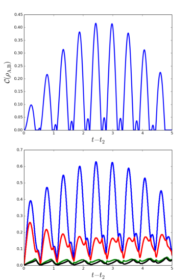
Figure 7: Upper panel: ${\cal C}[\rho_{{\rm{A}},{\rm{B}}}(t-t_{2})]$ for $g=1$, $h_{{\rm{A}}}=h_{{\rm{B}}}=0.25$, $S=5$, and a starting soliton with $\lambda_{\beta}=10$. Lower panel: eigenvalues $\{\mu_{1},\mu_{2},\mu_{3},\mu_{4}\}$ for the same parameters values as above. Cusps in the upper panel originates from the eigenvalues crossings seen in the lower panel.

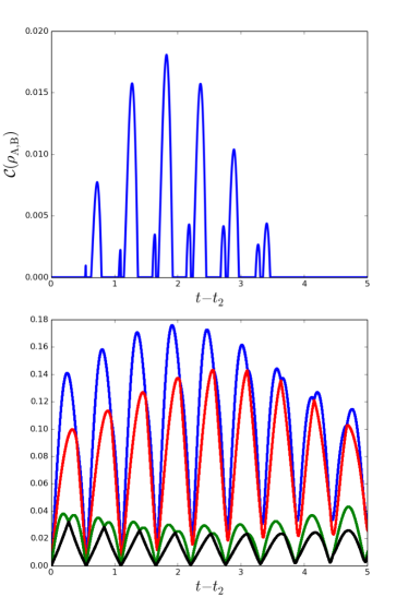
Figure 8: Same as in Fig. 7 for a starting soliton with $\lambda_{\beta}=2.5$.

VII Conclusions

The results presented in the previous sections show that a large-$S$ spin chain can be employed to generate entanglement between two distant qubits ${\rm{A}}$ and ${\rm{B}}$. The spin chain initially is in a classical-like state, corresponding to a running Heisenberg soliton passing by ${\rm{A}}$. In a first stage ${\rm{A}}$ interacts with the chain spin ${\bm{S}}_{{\rm{A}}}$, dynamically establishing quantum correlations which, in a second stage, the moving soliton can efficiently carry with to the location of the chain spin ${\bm{S}}_{{\rm{B}}}$, which in turn interacts with ${\rm{B}}$ in such a way that finally the system of the two qubits is in an entangled state.

The one-to-one mapping between the classical spin chain configurations and the tensor product of single-spin coherent states, allowed us to approximate the quantum evolution of the chain. However, in order to obtain the final quantum state, several classical-like evolutions must be superposed, as after the first stage ${\bm{S}}_{{\rm{A}}}$ is no more in a definite coherent state: such a simultaneous existence of ‘parallel classical histories’ explains why a classical-like description of the chain dynamics can account for quantum correlation transfer.

The explicit calculations have been made feasible by the introduction of simplifying assumptions. The first one concerns the time dependence of the qubit-chain interactions, which implies the ability to somehow switch on and off the interaction in a very short time: although this is a typical approximation in theoretical schemes, it is not always clear how to implement it in diverse realizations, especially for solid-state devices. The onset of the entangling dynamics between ${\rm{A}}$ and ${\bm{S}}_{{\rm{A}}}$, and later on between ${\rm{B}}$ and ${\bm{S}}_{{\rm{B}}}$, in the terms described in Secs. III and VI, can be thought to be embedded in the original model: in fact, before the soliton arrival all spins and the qubits are in the up state, so the interactions act trivially, giving an overall phase factor; only when the incoming soliton modifies the state of ${\bm{S}}_{{\rm{A}}}$, a non trivial dynamics of the (${\rm{A}}$,${\bm{S}}_{{\rm{A}}}$) subsystem is induced; in a similar way, the relevant dynamics of the subsystem(${\rm{B}}$,${\bm{S}}_{{\rm{B}}}$) only starts when the partially deformed soliton, reaches ${\bm{S}}_{{\rm{B}}}$. This would effectively be tantamount to switching on the couplings between the qubits and the chain, although not abruptly as in Eq. (4), and it is not to be expected to yield dramatic changes in the qualitative behavior. A suitable mechanism for finally quenching the interactions can also be imagined, as for instance that proposed in HeintzeEtal13 .

A further simplification was to assume the chain to be ‘frozen’ during the evolutions of the pairs $({\rm{A}},{\bm{S}}_{{\rm{A}}})$ and $({\rm{B}},{\bm{S}}_{{\rm{B}}})$ (first and third dynamical stage), i.e., that the typical time-scale of the qubit-spin interaction, $(gS)^{-1}$, be much smaller than that of the chain dynamics associated to the propagating soliton, given by $\tau_{\beta}=(JS\,h\,\sin\!2\beta)^{-1}$ (see Appendix A), namely,

$${J\over g}{h\sin 2\beta}\ll 1~{}.$$ (45)

The above relation can be satisfied both if $g\gg J$, i.e., the chain coupling is much weaker than the qubit-spin coupling, or if $h\simeq\mu_{B}H/JS\ll 1$, i.e., the intensity $H$ of the uniform field applied to the chain is weak compared with the chain coupling. This second requirement is usually met if the spin chain is thought to be some solid-state system, as typically exchange energies are much larger than Zeeman energies.

In virtue of the described results we conclude that, by choosing suitable values of the tunable parameters and the initial state, a large-$S$ spin chain can realize a two-qubit entangling gate. The carriers of quantum correlations, i.e., solitons, are known to be robust against noise and external disturbances, and make the hybrid scheme we have proposed a promising alternative to the most commonly studied purely quantum buses.

Appendix A Heisenberg solitons

Let us consider a classical spin-$S$ Heisenberg chain, i.e., a 1D array of (spin-)vectors $\bm{S}_{n}\equiv{S}\,\bm{s}_{n}$, whose magnitude $S$ has the dimension of an action. The unit vectors $\bm{s}_{n}$ are naturally parametrized by polar coordinates, $\bm{s}_{n}\equiv(\sin\theta_{n}\cos\varphi_{n},\sin\theta_{n}\sin\varphi_{n},\cos\theta_{n})$, with $\varphi_{n}$ and $\cos\theta_{n}$ canonically conjugated variables, $\{\varphi_{n},\cos\theta_{l}\}=S^{-1}\,\delta_{nl}$. Its Hamiltonian is the classical analogue of Eq. (3):

$${\cal H}_{\rm cl}=-JS^{2}{\sum}_{n}\bm{s}_{n}{\cdot}\bm{s}_{n+1}-\gamma S\bm{H}{\cdot}{\sum}_{n}\bm{s}_{n}~{},$$ (46)

and the corresponding EoM for the unit vectors $\bm{s}_{n}$ are

$$\partial_{t}\bm{s}_{n}=JS\,\bm{s}_{n}\times(\bm{s}_{n+1}{+}\bm{s}_{n-1}+\bm{h})~{},$$ (47)

where $JS$ sets the frequency scale and $\bm{h}\equiv\gamma\bm{H}/(JS)$ is the dimensionless Zeeman field.

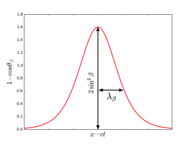
Figure 9: TW soliton:  $1-\cos\theta_{\beta}(\xi)$ for $\tan\!\beta\,{=}\,2$.

As shown by Tjon and Wright TjonW1977 (TW), the Heisenberg chain EoM have, in the continuum approximation (lattice spacing $d\,{\to}\,0$), an analytical ‘one-soliton’ solution of the form:

$$\left\{\begin{aligned} \theta_{\beta}&=2\sin^{-1}(\sin\!\beta\,\operatorname{sech}\xi)~{},\\ \varphi_{\beta}&=\varphi_{0}+\cot\!\beta\,\xi+\tan^{-1}(\tan\!\beta\,\tanh\xi)~{},\end{aligned}\right.$$ (48)

where $\xi\equiv\,(x{-}vt)/\lambda_{\beta}$ and $x\,{=}\,nd$ is the ‘continuum’ coordinate. The soliton amplitude, characterized by the dimensionless parameter $\beta\in(0,\pi/2)$ ($\theta\,{\leq}\,2\beta$) is related with the soliton velocity $v$ by $\cos\!\beta=v/({2dJS\sqrt{h}})$, and determines the soliton length  $\lambda_{\beta}=d/({\sqrt{h}\sin\!\beta})$ , time scale  $\tau_{\beta}=(JS\,h\,\sin\!2\beta)^{-1}$ , and energy  $\varepsilon_{\beta}=8JS^{2}\sqrt{h}\,\sin\!\beta$ . Fig. 9 reports a typical TW soliton, and it is useful to note that solitons with larger amplitude $\beta$ have larger energy ($\sim\sin\!\beta$), are narrower $(\sim 1/\sin\!\beta)$ and slower ($\sim\cos\!\beta$). Although there are no known analytic soliton solutions of the discrete model, the continuum approximation holds for configurations that vary slowly on the scale of the lattice spacing $d$, so that the solution (48) approximately applies also to the chain model (46) provided that $\lambda_{\beta}\gg{d}$, i.e., $\sqrt{h}~{}\sin\!\beta\,{\ll}\,1$. This is generally true in real systems, whose typical exchange energies are of the order of tenths-hundreds of Kelvin degrees: as $\mu_{\rm{B}}=0.67$ K/Tesla, only very large fields could break the inequality. Numerical investigations confirmed that soliton-like excitations can be injected in discrete spin chains and propagate along them without substantial distortion CNVV2015a .

Appendix B Spin coherent states

The states of a spin-$S$ particle are usually expanded on the basis of the $2S{+}1$ eigenvectors of the $z$-component of the spin operator, $\hat{S}^{z}|{m}\rangle=m|{m}\rangle$, with $m=-S,\,...,S$. Given an arbitrary direction ${\bm{s}}$ in 3D space, i.e., a unit vector ${\bm{s}}\equiv(\sin\theta\cos\varphi,\sin\theta\sin\varphi,\cos\theta)$ defined by its spherical angles $\{\theta,\varphi\}\equiv\Omega$, the corresponding spin coherent state $|{\Omega}\rangle$ is defined as

$$|{\Omega}\rangle=\big{(}\cos{\textstyle\frac{\theta}{2}}\big{)}^{2S}\,\exp\Big{(}\tan{\textstyle\frac{\theta}{2}}\,e^{i\varphi}\,\hat{S}^{-}\Big{)}|{S}\rangle~{},$$ (49)

$|{S}\rangle$ being the eigenvector of $\hat{S}^{z}$ with maximal eigenvalue, $m{=}S$. This state can also be written in the usual basis of eigenstates of $\hat{S}^{z}$:

$$|{\Omega}\rangle=\sum_{m=-S}^{S}\langle{m}|{\Omega}\rangle|{m}\rangle\,,$$ (50)

the coefficients in this relation being the overlaps between the eigenvectors $|{m}\rangle$ and the coherent state $|{\Omega}\rangle$,

$$\langle{m}|{\Omega}\rangle = \big{(}\cos{\textstyle\frac{\theta}{2}}\big{)}^{2S}\sqrt{\textstyle\frac{2S!}{(S{-}m)!(S{+}m)!}}$$ (51)

$$~{}~{}~{}~{}~{}~{}~{}~{}\times~{}\big{(}\tan{\textstyle\frac{\theta}{2}}\big{)}^{(S-m)}e^{i(S-m)\varphi}~{}.$$

An important property of spin coherent states is that the expectation values of the spin-component operators are equal to the components of a classical vector of modulus $S$ oriented along ${\bm{s}}$, i.e.,

$$\langle{\Omega|\hat{\bm{S}}}|{\Omega}\rangle=S(\sin\theta\cos\varphi,\sin\theta\sin\varphi,\cos\theta)=S\,{\bm{s}}~{}.$$ (52)

Spin coherent states form a non-orthogonal and overcomplete set of states. Indeed,

$$\langle{\Omega^{\prime}}|{\Omega}\rangle=\Big{(}\cos{\textstyle\frac{\theta}{2}}\cos{\textstyle\frac{\theta^{\prime}}{2}}+\sin{\textstyle\frac{\theta}{2}}\sin{\textstyle\frac{\theta^{\prime}}{2}}\,e^{i(\varphi-\varphi^{\prime})}\Big{)}^{2S}\,,$$ (53)

which implies

$$\big{|}\langle{\Omega^{\prime}}|{\Omega}\rangle\big{|}^{2}=\Big{(}{\textstyle\frac{1+{\Omega}\cdot{\Omega}^{\prime}}{2}}\Big{)}^{2S}=\Big{(}\cos{\textstyle\frac{\widehat{\Omega\Omega^{\prime}}}{2}}\Big{)}^{4S}~{},$$ (54)

i.e., the overlap modulus depends on the angle $\widehat{\Omega\Omega^{\prime}}$ between the directions identified by $\Omega$ and $\Omega^{\prime}$, respectively. The (over)completeness relation reads

$$(2S{+}1)\int\frac{d\Omega}{4\pi}\,|{\Omega}\rangle\langle{\Omega}|=\mathds{1}_{S}~{},$$ (55)

where $d\Omega={d\cos\theta}~{}{d\varphi}$.

From Eq. (54) we see that $\big{|}\langle{\Omega^{\prime}}|{\Omega}\rangle\big{|}^{2}\propto\delta(\Omega-\Omega^{\prime})$ in the limit $S\to\infty$, and reminding Eq. (52) and the description of the classical Heisenberg chain given in Appendix A, it clearly appears that the spin coherent states are the tool of choice to properly address the classical limit of spin systems.

References

- (1) S. Bose, Phys. Rev. Lett., 91, 207901 (2003).
- (2) L. Campos Venuti, S.M. Giampaolo, F. Illuminati, and P. Zanardi, Phys. Rev. A., 76, 052328 (2007),
- (3) L. Banchi, A. Bayat, P. Verrucchi, and S. Bose, Phys. Rev. Lett., 106, 140501 (2011).
- (4) S. Campbell, T. J. G. Apollaro, C. Di Franco, L. Banchi, A. Cuccoli, R. Vaia, F. Plastina, and M. Paternostro, Phys. Rev. A, 84, 052316 (2011).
- (5) T. J. G. Apollaro, L. Banchi, A. Cuccoli, R. Vaia, and P. Verrucchi, Phys. Rev. A, 85, 052319 (2012).
- (6) S. Paganelli, S. Lorenzo, T. J. G. Apollaro, F. Plastina, and G. L. Giorgi, Phys. Rev. A, 87, 062309 (2013).
- (7) A. Kay, Int. J. Quant. Inf. 8, 641 (2010).
- (8) P. Karbach and J. Stolze, Phys. Rev. A 72, 030301 (2005).
- (9) M. Christandl, N. Datta, A. Ekert, and A. J. Landahl, Phys. Rev. Lett. 92, 187902 (2004).
- (10) M.-H. Yung and S. Bose Phys. Rev. A 71, 032310 (2005).
- (11) C. Di Franco, M. Paternostro, and M. S. Kim, Phys. Rev. Lett. 101, 230502 (2008).
- (12) M. H. Ahmed and A. D. Greentree Phys. Rev. A 91, 022306 (2015).
- (13) A. Zwick, G. A. Álvarez, J. Stolze, and O. Osenda, Phys. Rev. A 84, 022311 (2011).
- (14) Y. Wang, F. Shuang, and H. Rabitz, Phys. Rev. A 84, 012307 (2011).
- (15) A. Cuccoli, D. Nuzzi, R. Vaia, and P. Verrucchi, J. Appl. Phys. 115, 17B302 (2014).
- (16) A. Cuccoli, D. Nuzzi, R. Vaia, and P. Verrucchi, New J. Phys. 17, 083053 (2015).
- (17) A. M. Perelomov, Generalized coherent states and their applications, Springer-Verlag (1986).
- (18) W.-M. Zhang, D. H. Feng, and R. Gilmore, Rev. Mod. Phys. 62, 867 (1990).
- (19) D. Calvani, A. Cuccoli, N. I. Gidopoulos, and P. Verrucchi, Proc. Natl. Acad. Sci., 110(17), 6748-6753 (2013)
- (20) R. Balakrishnan, A. R. Bishop, Phys. Rev. B 40, 9194 (1989).
- (21) L. Diósi, W. T. Strunz, Phys. Lett. A 235, 569 (1997).
- (22) J. Helm, W. T. Strunz, S. Rietzler, and L. E. Würflinger Phys. Rev. A 83, 042103 (2011).
- (23) M. Combescure, J. Math. Phys. 33, 3870 (1992).
- (24) E. H. Lieb, Commun. Math. Phys. 31(4), 327-340 (1973).
- (25) L. G. Yaffe, Rev. Mod. Phys. 54, 407-435 (1982).
- (26) J. Tjon and J. Wright, Phys. Rev. B 15, 3470 (1977).
- (27) L. A. Takhtajan, Phys. Lett. A 64, 235 (1977).
- (28) The validity of this approximation in a realistic setup sets constraints on the ratios of the interaction constants , and the spin-chain time scale; nevertheless, this extreme simplification is aimed at demonstrating the possibility of entanglement transfer by a quasi-classical channel.
- (29) J. M. Radcliffe, J. Phys. A 4, 313 (1971).
- (30) The Von Neumann entropy of with is given by with . Since the rest of the system is factorized at this stage of the evolution, correctly quantifies the entanglement between and .
-
(31)
The evolution of the initial state is evaluated exactly by the numerical diagonalization of the Hamiltonian (2); numerical calculations are performed using the basis of the and eigenvectors:
. - (32) W. K. Wootters, Phys. Rev. Lett. 80, 2245 (1998).
- (33) E. Heintze, F. El Hallak, C. Clauß, A. Rettori, M. G. Pini, F. Totti, M. Dressel & L. Bogani Nature Materials 12, 202–206 (2013)