Floquet control of dipolaritons in quantum wells

Abstract

We developed the theory of dipolaritons in semiconductor quantum wells irradiated by an off-resonant electromagnetic wave (dressing field). Solving the Floquet problem for the dressed dipolaritons, we demonstrated that the field drastically modifies all dipolaritonic properties. In particular, the dressing field strongly effects on terahertz emission from the considered system. The described effect paves the way for optical control of prospective dipolariton-based terahertz devices.

I Introduction

Advances in laser and microwave techniques made possible the use of high-frequency fields as tools to control both atomic and condensed-matter structures (so-called “Floquet engineering” based on the Floquet theory of periodically driven quantum systems Hanggi_98 ; Bukov2015 ; Blanes2009 ). As a consequence, properties of electrons strongly coupled to an electromagnetic field — also known as “electrons dressed by the field” (dressed electrons) — are currently in the focus of attention of the scientific community. Recently, the physical characteristics of dressed electrons were analyzed for various nanostructures, including quantum wells Wagner_10 ; Teich_13 ; Morina_15 ; Dini_16 , quantum rings Sigurdsson_14 ; Joibari_14 ; Koshelev_15 , graphene Perez_14 ; Glazov_14 ; Kibis_16 ; Kristinsson_16 , etc. Developing this scientific trend at the border of quantum optics and physics of nanostructures, we present the theory of dressed dipolaritons in semiconductor quantum wells (QWs).

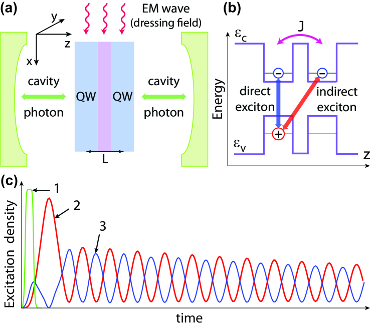
Figure 1: Sketch of the system under consideration: (a) Two tunnel-coupled semiconductor QWs with the inter-QW distance $L$, which are embedded into a microcavity and irradiated by an off-resonant electromagnetic wave (dressing field) incident along the $x$ axis and linearly polarized along the $z$ axis; (b) Structure of excited electron-hole pairs (direct and indirect excitons) in QWs, where $\varepsilon_{c}$ is the conduction band, $\varepsilon_{v}$ is the valence band, and $J$ denotes the tunnel coupling of the QWs; (c) Density of excited cavity photons (curve 1), which results in oscillations of indirect and direct exciton densities (curves 2 and 3, respectively).

Generally, polaritons are quasiparticles arisen from the strong coupling between matter excitations and photons inside a microcavity (see, e.g., Refs. KavokinBook ; CarusottoRev ; DengRev ). They can be controlled with different methods, including the electrical tuning of the polarization Dreismann2016 and energy Tsotsis2014 , the spatial tuning of the polariton condensate by the excitonic reservoir engineering Askitopoulos2013 , the AC Stark tuning of the energy of polariton modes Hayat2012 ; Cancellieri2014 ; Sie2015 , and others. If tunnel-coupled semiconductor QWs are embedded into a microcavity (see Fig. 1a), the strong coupling between photons in the cavity and excitons in the QWs results in the formation of a particular kind of polaritons known as dipolaritons Cristofolini2012 . The energy band structure hosting the dipolariton is pictured schematically in Fig. 1b. The absorption of cavity photon excites an electron-hole pair in a QW. In turn, the Coulomb attraction between an electron and a hole forms a bound state (direct exciton) confined in the same QW. Since there is the tunnel coupling, $J$, between the two QWs, the conduction electron can jump to the neighboring QW. The tunneling results in the electron-hole pair confined in different QWs (indirect exciton) which does not interact with cavity photons but couples to the direct exciton (see, e.g., Refs. High2012 ; ButovRev ; Muljarov2012 ; Christmann2011 ). Thus, dipolariton is the three-component quasiparticle consisting from the direct exciton, the indirect exciton and the cavity photon.

After the first experimental observation of dipolaritons Cristofolini2012 , it was demonstrated that they have distinct response to electric and magnetic fields Wilkes2016 and stronger interparticle interaction as compared to conventional polaritons Byrnes2014 . Moreover, they can be used for enhanced electrical control Rosenberg2016 ; Li2015 , facilitate indirect exciton condensate preparation Shahnazaryan2015 , single photon emission Kyriienko2014 , and other optoelectronic applications. Particularly, it was predicted that dipolaritons can serve as an efficient terahertz emission source Kyriienko2013 ; Kristinsson2013 ; Kristinsson2014 . Namely, an excitation of the cavity photon mode by an optical pulse (curve 1 in Fig. 1c) results in oscillations of indirect and direct exciton densities (curves 2 and 3 in Fig. 1c, respectively) with the THz frequency. It should be noted that indirect excitons have large dipole moment along the $z$ axis, $d_{z}\approx eL$, where $e$ is the electron charge and $L$ is the effective distance between the centers of QWs (see Fig. 1a). Therefore, the oscillations of the exciton density lead to the emission of electromagnetic waves in the THz range.

Currently, the search for effective sources of THz emission is one of the most exciting scientific trends at the border of applied and fundamental physics. However, the use of dipolaritons as a source of THz radiation needs effective methods to tune the THz emission from dipolariton systems. In the present Letter, we develop the theory of the optical control of dipolaritons with an off-resonant laser excitation (dressing field), which creates physical basis for such a tuning.

II Model

Let us consider the conventional dipolariton setup consisting of two tunnel-coupled semiconductor QWs embedded into a microcavity Cristofolini2012 . Additionally, we assume the QWs to be irradiated by an off-resonant electromagnetic wave (dressing field) incident along the $x$ axis and linearly polarized along the $z$ axis (see Fig. 1a). It should be noted that the cavity mirrors do not effect the propagation of the dressing electromagnetic wave because of the chosen wave orientation. The dressed dipolaritons in the QWs can be described by the time-dependent Hamiltonian

$$\hat{\cal H}(t) = \hbar\omega_{1}\hat{a}^{\dagger}_{1}\hat{a}_{1}+\hbar\omega_{2}\hat{a}^{\dagger}_{2}\hat{a}_{2}+\hbar\omega_{3}\hat{a}^{\dagger}_{3}\hat{a}_{3}$$ (1)

$$+ \frac{\hbar\Omega_{R}}{2}(\hat{a}^{\dagger}_{1}\hat{a}_{2}+\hat{a}^{\dagger}_{2}\hat{a}_{1})+\frac{J}{2}(\hat{a}^{\dagger}_{2}\hat{a}_{3}+\hat{a}^{\dagger}_{3}\hat{a}_{2})$$

$$+ (d_{z}E\cos\omega t)\hat{a}^{\dagger}_{3}\hat{a}_{3}-\frac{(d_{cv}E\cos\omega t)^{2}}{2\hbar\delta}\hat{a}^{\dagger}_{2}\hat{a}_{2},$$

where $\hat{a}^{\dagger}_{j}$ and $\hat{a}_{j}$ are the creation and annihilation operators, respectively, for a cavity photon ($j=1$), a direct exciton ($j=2$), and an indirect exciton ($j=3$). The physical meaning of the seven terms of the Hamiltonian (1) is as follows: The first, second and third terms describe energies of noninteracting cavity photons, direct excitons and indirect excitons with the frequencies $\omega_{1,2,3}$, respectively; the fourth term describes the interaction between a cavity photon and a direct exciton, which results in the Rabi oscillations of this photon-exciton subsystem with the Rabi frequency, $\Omega_{R}$; the fifth term describes the tunnel coupling between direct and indirect excitons with the coupling energy, $J$; the sixth term describes the usual dipole interaction between an indirect exciton with the dipole moment, $d_{z}$, and the electric field of the wave, $E\cos\omega t$, which is actively studied in state-of-the-art experiments (see, e.g., Ref. ButovRev ); the seventh term describes the field-induced AC Stark shift of the direct exciton VonLehmen1986 ; Unold2004 . In contrast to the case of indirect exciton, the dipole moment of the direct exciton is very small. As a consequence, the dipole interaction between the direct exciton and the wave is negligible weak. That is why the physical origins of the sixth and seventh terms of the Hamiltonian (1) are substantially different. It should be noted also that the interband dipole moment, $d_{cv}$, is calculated with using atomic wave functions. Therefore, the seventh term almost does not depend on the orientation of the wave relative to the growth direction of QW. As to the first five terms of the Hamiltonian (1), they exactly coincide with the conventional Hamiltonian describing “bare” dipolaritons Cristofolini2012 .

To perform the Floquet analysis of the considered system, let us apply the unitary transformation

$$\hat{U}(t)=\exp\left[i\frac{\left(d_{cv}E\right)^{2}}{8\hbar^{2}\omega\delta}\sin 2\omega t\,\,\hat{a}^{\dagger}_{2}\hat{a}_{2}-i\frac{d_{z}E\sin\omega t}{\hbar\omega}\hat{a}^{\dagger}_{3}\hat{a}_{3}\right]$$

to the Hamiltonian (1). Then the transformed Hamiltonian of dressed dipolaritons, $\hat{\cal H}^{{}^{\prime}}(t)=\hat{U}^{\dagger}(t)\hat{\cal H}(t)\hat{U}(t)-i\hbar\hat{U}^{\dagger}(t)\partial_{t}\hat{U}(t)$, reads

$$\hat{\cal H}^{\prime}(t)=\hbar\omega_{1}\hat{a}^{\dagger}_{1}\hat{a}_{1}+\left[\hbar\omega_{2}-\frac{(d_{cv}E)^{2}}{4\hbar\delta}\right]\hat{a}^{\dagger}_{2}\hat{a}_{2}+\hbar\omega_{3}\hat{a}^{\dagger}_{3}\hat{a}_{3}$$

$$+\frac{J}{2}\cos\left[\frac{\left(d_{cv}E\right)^{2}}{8\hbar^{2}\omega\delta}\sin 2\omega t+\frac{d_{z}E\sin\omega t}{\hbar\omega}\right](\hat{a}^{\dagger}_{2}\hat{a}_{3}+\hat{a}^{\dagger}_{3}\hat{a}_{2})$$

$$+i\frac{J}{2}\sin\left[\frac{\left(d_{cv}E\right)^{2}}{8\hbar^{2}\omega\delta}\sin 2\omega t+\frac{d_{z}E\sin\omega t}{\hbar\omega}\right](\hat{a}^{\dagger}_{2}\hat{a}_{3}-\hat{a}^{\dagger}_{3}\hat{a}_{2})$$

$$+\frac{\hbar\Omega_{R}}{2}\cos\left[\frac{\left(d_{cv}E\right)^{2}}{8\hbar^{2}\omega\delta}\sin 2\omega t\right](\hat{a}^{\dagger}_{1}\hat{a}_{2}+\hat{a}^{\dagger}_{2}\hat{a}_{1})$$

$$+i\frac{\hbar\Omega_{R}}{2}\sin\left[\frac{\left(d_{cv}E\right)^{2}}{8\hbar^{2}\omega\delta}\sin 2\omega t\right](\hat{a}^{\dagger}_{1}\hat{a}_{2}-\hat{a}^{\dagger}_{2}\hat{a}_{1}).$$ (2)

Within the conventional Floquet theory for periodically driven quantum systems, the time-dependent Hamiltonian (II) can be expanded into the power series of the inverse frequency, $(1/\omega)^{n}$, where $n=0,1,2,...$ (the Floquet-Magnus expansion Bukov2015 ; Blanes2009 ). Assuming the dressing field to be high-frequency, $\omega\gg\Omega_{R},J/\hbar$, one can restrict the expansion to the zeroth-order term ($n=0$) which is given by the Hamiltonian (II) averaged over the field period, $T=2\pi/\omega$. As a result, we arrive from the time-dependent Hamiltonian (II) at the effective time-independent Hamiltonian of dressed dipolaritons, $\hat{\cal H}_{0}=(1/T)\int_{0}^{T}\hat{\cal H}^{\prime}(t)dt$, which reads

$$\hat{\cal H}_{0} = \hbar\omega_{1}\hat{a}^{\dagger}_{1}\hat{a}_{1}+\hbar\widetilde{\omega}_{2}\hat{a}^{\dagger}_{2}\hat{a}_{2}+\hbar\omega_{3}\hat{a}^{\dagger}_{3}\hat{a}_{3}$$ (3)

$$+ \frac{\hbar\widetilde{\Omega}_{R}}{2}(\hat{a}^{\dagger}_{1}\hat{a}_{2}+\hat{a}^{\dagger}_{2}\hat{a}_{1})+\frac{\widetilde{J}}{2}(\hat{a}^{\dagger}_{2}\hat{a}_{3}+\hat{a}^{\dagger}_{3}\hat{a}_{2}),$$

where

$$\widetilde{\omega}_{2}=\omega_{2}-\frac{(d_{cv}E)^{2}}{4\hbar^{2}\delta},$$ (4)

$$\widetilde{J}=\frac{J}{T}\int_{0}^{T}\exp\left[i\frac{\left(d_{cv}E\right)^{2}}{8\hbar^{2}\omega\delta}\sin 2\omega t+i\frac{d_{z}E\sin\omega t}{\hbar\omega}\right]dt,$$ (5)

$$\widetilde{\Omega}_{R}=\frac{\Omega_{R}}{T}\int_{0}^{T}\exp\left[i\frac{\left(d_{cv}E\right)^{2}}{8\hbar^{2}\omega\delta}\sin 2\omega t\right]dt.$$ (6)

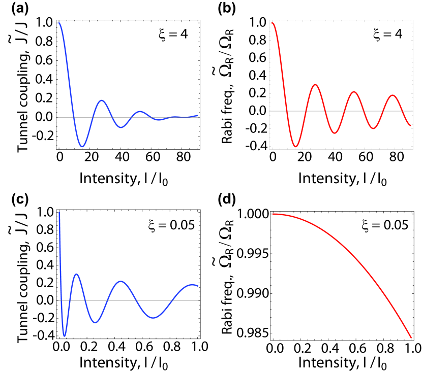
Figure 2: Dependencies of the renormalized tunnel coupling, $\widetilde{J}$, and Rabi frequency, $\widetilde{\Omega}_{R}$, on the irradiation intensity, $I$, for different values of the dipolariton-field coupling parameter, $\xi$. The intensity is plotted in the units of $I_{0}=\hbar^{2}|\delta|\omega c\epsilon_{0}/d_{cv}^{2}$.

The Hamiltonian of dressed dipolaritons (3) exactly coincides with the stationary Hamiltonian of “bare” dipolaritons described by the first five terms of the Hamiltonian (1) with the replacements $\omega_{2}\rightarrow\widetilde{\omega}_{2}$, $\Omega_{R}\rightarrow\widetilde{\Omega}_{R}$ and $J\rightarrow\widetilde{J}$. Therefore, the quantities (4)–(6) should be treated as stationary dipolariton parameters renormalized by the dressing field.

III Discussion and conclusions

First of all, let us discuss the dependence of the parameters (4)–(6) on the dressing field amplitude, $E$, and the frequency, $\omega$, restricting the consideration to the case of the red-detuned dressing field ($\delta<0$). The field-induced renormalization of the direct exciton frequency (4) is described by the known dynamic Stark shift VonLehmen1986 . As to the renormalized parameters $\widetilde{J}$ and $\widetilde{\Omega}_{R}$, the exponential functions in Eqs. (5)—(6) contain the two different terms which are squared and linear in the field amplitude, $E$. Physically, the first of them arises from the dressing of direct excitons, whereas the second one is caused by the dressing of indirect excitons. The coupling parameter of the first dressing depends on the interband dipole moment, $d_{cv}$, and the detuning, $\delta$, whereas the second one is described by the inter-QW dipole moment, $d_{z}$. Therefore, it is reasonable to introduce the dimensionless dipolariton-field coupling parameter, $\xi=(d_{cv}/d_{z})\sqrt{\omega/2|\delta|}$, which describes the relative contribution of these two different dressing mechanisms to the renormalization of dipolaritonic properties. This parameter can be controlled by varying the inter-QW distance, $L$, and the detuning, $\delta$. Particularly, the state-of-the-art semiconductor technologies can easily fabricate QWs with the broad range of the dipole moments, $0<d_{cv}/d_{z}<10$. Dependencies of the renormalized tunnel coupling, $\widetilde{J}$, and the renormalized Rabi frequency, $\widetilde{\Omega}_{R}$, on the irradiation intensity, $I$, are plotted in Fig. 2 for different values of the parameter $\xi$. We see that both tunnel coupling and the Rabi frequency oscillate as functions of the irradiation intensity. Mathematically, these oscillations arise from periodical functions in Eqs. (5)–(6). It follows from Eq. (6) that the renormalization of the Rabi frequency, $\widetilde{\Omega}_{R}$, is described by the interband dipole moment, $d_{cv}$, which does not depend on the sample size, $L$. Therefore, the Rabi frequency, $\widetilde{\Omega}_{R}$, does not depend on the parameter $\xi$ for a given semiconductor material (see Figs. 2b and 2d). On the contrary, the renormalized tunnel coupling (5) depends on both the interband dipole moment, $d_{cv}$, and the inter-QW dipole moment, $d_{z}$. Applying the well-known Jacobi-Anger expansion to transform the exponential function in Eq. (5), we arrive at the simple expression, $\widetilde{J}\approx J\mathcal{J}_{0}\left({d_{z}E}/{\hbar\omega}\right)$, describing the tunnel coupling for $\xi\ll 1$, where $\mathcal{J}_{0}$ is the zeroth-order Bessel function of the first kind. It follows from this that the decrease of $d_{z}$ leads to decreasing the period of oscillations of the tunnel coupling, $\widetilde{J}$, as a function of the field intensity, $I$ (see Fig. 2a and 2c). One can conclude that the dressing field changes the intrinsic parameters of the dipolariton, $J$ and $\Omega_{R}$, whereas the alternative approach to control polaritonic systems by the interaction with reservoir excitons results in changing dipolariton dynamics (see, e.g., Ref. Askitopoulos2013 ). Thus, these two methods of dipolariton control supplement each other and can be combined in experiments.

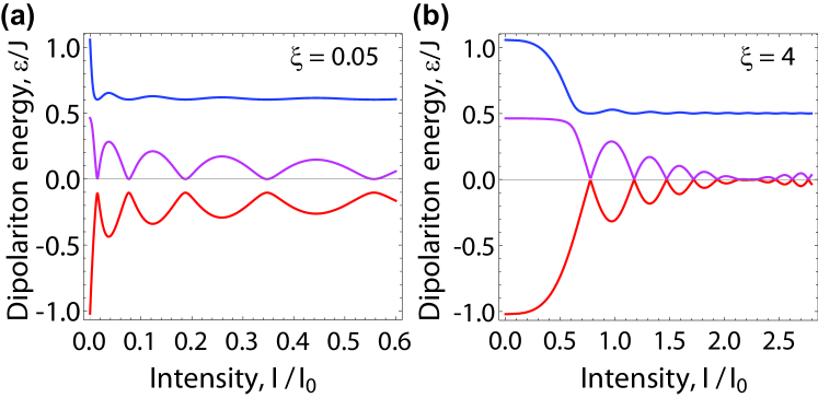
Figure 3: The energy spectrum of dressed dipolariton, $\varepsilon$, as a function of the dressing field intensity, $I$, for $\omega_{1}=0.5J$, $\widetilde{\omega}_{2}=\omega_{3}=0$, $\Omega_{R}=0.25J$.

The discussed renormalization of the parameters (4)–(6) by a dressing field results in the renormalization of all physical properties of the dipolariton system. Diagonalizing the Hamiltonian (II), we can calculate numerically the energy spectrum of dressed dipolaritons, which is shown in Fig. 3. We observe that the energy spectrum consists of three energy levels which depend differently on the dressing field intensity, $I$. Particularly, the dressing field decreases the gap between the two lowest dipolariton energies (see Fig. 3a) and can turn the gap into zero (see Fig. 3b). In order to calculate the spectrum of electromagnetic emission from the dipolariton system, we have to consider the dynamics of the system under the pulsed excitation of the cavity mode (see curve 1 in Fig. 1c) with an external source at the frequency $\omega_{0}$. Introducing the detuning parameters for the photon-exciton modes of the cavity, $\Delta_{1,2,3}=\hbar(\omega_{1,2,3}-\omega_{0})$, we can perform the Fourier analysis of the oscillations of exciton densities within the approach used in Refs. Kyriienko2013 ; Kristinsson2014 . For definiteness, let us focus on the dipolariton spectra of GaAs-based QWs with the interband dipole moment $d_{cv}=28$ Debay and the exciton energy $\hbar\omega_{2}=1.54$ eV, which are dressed by the field with the frequency $\omega/2\pi=10^{13}$ Hz. As a result, one can calculate numerically the spectrum of electromagnetic emission from the excited dipolariton system, which is plotted in Fig. 4. The spectrum consists of the main spectral line and the two sideband spectral lines (see Fig. 4a). For typical samples, the tunnel coupling, $J$, is of meV scale Cristofolini2012 . Thus, the main spectral line corresponds to the terahertz emission (see Fig. 4b). It should be noted that one can construct a single-mode terahertz emitter if the sideband modes are suppressed with an additional THz cavity Kristinsson2014 . In the most relevant case of $\xi\ll 1$, the photon energies corresponding to the main line and the sideband lines can be described adequately by the expressions $\hbar\Omega\approx\widetilde{J}$ and $\hbar\Omega\approx\Delta_{1}\pm\widetilde{J}$, respectively. Therefore, we can write the frequency of terahertz emission corresponding to the main spectral line, $\Omega$, as $\hbar\Omega\approx J\mathcal{J}_{0}\left({d_{z}E}/{\hbar\omega}\right).$ This means that the terahertz emission from the dipolariton system is controlled by the dressing field amplitude, $E$, and the dressing field frequency, $\omega$. Particularly, varying the irradiation intensity, $I$, one can tune the terahertz frequency, $\Omega$ (see Fig. 4b).

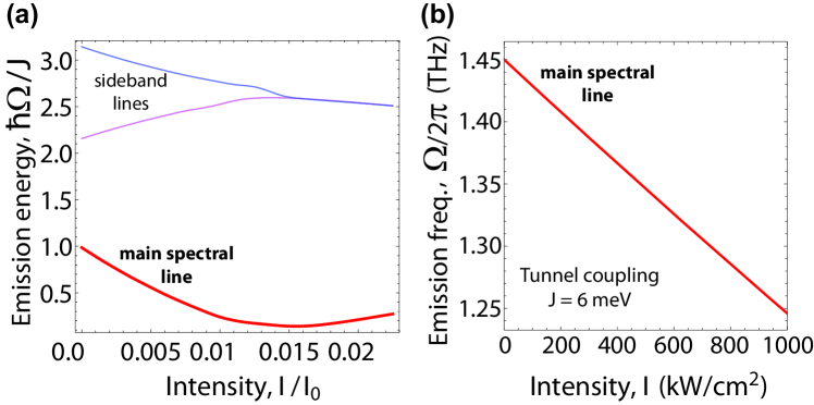
Figure 4: Spectrum of electromagnetic emission, $\Omega$, from a dipolariton system in GaAs-based QWs with the detuning $\Delta_{1}=2.5J$, $\Delta_{2}=\Delta_{3}=0$, and the Rabi frequency $\Omega_{R}=J$, as a function of irradiation intensity, $I$: (a) Photon energy of the emission corresponding to the main and sideband spectral lines; (b) Frequency of the terahertz emission.

Summarizing the aforesaid, one can conclude that an off-resonant high-frequency electromagnetic field (dressing field) can be used as an effective tool to control all physical properties of dipolaritons in semiconductor QWs, including their energy spectrum and dynamics. Particularly, the field-induced renormalization of the coupling of direct and indirect excitons results in changing terahertz emission from the dipolariton system. Since light-controlled electronic devices are typically much faster than those of electrically controlled, the proposed optical control of dipolaritonic terahertz emitters is expected to be faster than the usual gate control. Thus, the elaborated theory provides the ground for novel optoelectronic devices operated by light.

IV Funding

RISE Program (CoExAN); FP7 ITN Program (NOTEDEV); Russian Foundation for Basic Research (17-02-00053); Rannis (163082-051); Ministry of Education and Science of Russian Federation (3.4573.2017/6.7, 3.2614.2017/4.6, 14.Y26.31.0015); ERC QIOS (306576).

References

- (1) P. Hänngi, Driven quantum systems, in Quantum Transport and Dissipation edited by T. Dittrich, P. Hänggi, G.-L. Ingold, B. Kramer, G. Schön, and W. Zwerger (Wiley, Weinheim, 1998).
- (2) M. Bukov, L. D’Alessio, and A. Polkovnikov, Adv. Phys. 64, 139–226 (2015).
- (3) S. Blanes, F. Casas, J. A. Oteo, and J. Ros, Phys. Rep. 470, 151–238 (2009).
- (4) M. Wagner, H. Schneider, D. Stehr, S. Winnerl, A. M. Andrews, S. Schartner, G. Strasser, and M. Helm, Phys. Rev. Lett. 105, 167401 (2010).
- (5) M. Teich, M. Wagner, H. Schneider, and M. Helm, New J. Phys. 15, 065007 (2013).
- (6) S. Morina, O. V. Kibis, A. A. Pervishko, and I. A. Shelykh, Phys. Rev. B 91, 155312 (2015).
- (7) K. Dini, O. V. Kibis, I. A. Shelykh, Phys. Rev. B 93, 235411 (2016).
- (8) H. Sigurdsson, O. V. Kibis, I. A. Shelykh, Phys. Rev. B 90, 235413 (2014).
- (9) F. K. Joibari, Ya. M. Blanter, G. E. W. Bauer, Phys. Rev. B 90, 155301 (2014).
- (10) K. L. Koshelev, V. Yu. Kachorovskii, M. Titov, Phys. Rev. B 92, 235426 (2015).
- (11) P. M. Perez-Piskunow, G. Usaj, C. A. Balseiro, L. E. F. Foa Torres, Phys. Rev. B 89, 121401(R) (2014).
- (12) M. M. Glazov, S. D. Ganichev, Phys. Rep. 535, 101 (2014).
- (13) O. V. Kibis, S. Morina, K. Dini, I. A. Shelykh, Phys. Rev. B 93, 115420 (2016).
- (14) K. Kristinsson, O. V. Kibis, S. Morina, I. A. Shelykh, Sci. Rep. 6, 20082 (2016).
- (15) A. V. Kavokin, J. J. Baumberg, G. Malpuech, and F. P. Laussy, Microcavities (Oxford University Press, Oxford, 2007).
- (16) I. Carusotto and C. Ciuti, Rev. Mod. Phys. 85, 299 (2013).
- (17) H. Deng, H. Haug, and Y. Yamamoto, Rev. Mod. Phys. 82, 1489 (2010).
- (18) A. Dreismann, H. Ohadi, Y. del Valle-Inclan Redondo, R. Balili, Y. G. Rubo, S. I. Tsintzos, G. Deligeorgis, Z. Hatzopoulos, P. G Savvidis, and J. J. Baumberg, Nat. Mater. 15, 1074-1078 (2016).
- (19) P. Tsotsis, S. I. Tsintzos, G. Christmann, P. G. Lagoudakis, O. Kyriienko, I. A. Shelykh, J. J. Baumberg, A. V. Kavokin, Z. Hatzopoulos, P. S. Eldridge, and P. G. Savvidis, Phys. Rev. Appl. 2, 014002 (2014).
- (20) A. Askitopoulos, H. Ohadi, A. V. Kavokin, Z. Hatzopoulos, P. G. Savvidis, and P. G. Lagoudakis, Phys. Rev. B 88, 041308(R) (2013).
- (21) A. Hayat, C. Lange, L. A. Rozema, A. Darabi, H. M. van Driel, A. M. Steinberg, B. Nelsen, D. W. Snoke, L. N. Pfeiffer, and K. W. West, Phys. Rev. Lett. 109, 033605 (2012).
- (22) E. Cancellieri, A. Hayat, A. M. Steinberg, E. Giacobino, and A. Bramati, Phys. Rev. Lett. 112, 053601 (2014).
- (23) E. J. Sie, J. W. McIver, Yi-Hsien Lee, L. Fu, J. Kong, and N. Gedik, Nature Materials 14, 290-294 (2015).
- (24) P. Cristofolini, G. Christmann, S. I. Tsintzos, G. Deligeorgis, G. Konstantinidis, Z. Hatzopoulos, P. G. Savvidis, and J. J. Baumberg, Science 336, 704–707 (2012).
- (25) A. A. High, J. R. Leonard, A. T. Hammack, M. M. Fogler, L. V. Butov, A. V. Kavokin, K. L. Campman, and A. C. Gossard, Nature 483, 584C588 (2012).
- (26) L. V. Butov, J. Phys.: Condens. Matt. 19, 295202 (2007).
- (27) K. Sivalertporn, L. Mouchliadis, A. L. Ivanov, R. Philp, and E. A. Muljarov, Phys. Rev. B 85, 045207 (2012).
- (28) G. Christmann, A. Askitopoulos, G. Deligeorgis, Z. Hatzopoulos, S. I. Tsintzos, P. G. Savvidis, and J. J. Baumberg, Appl. Phys. Lett. 98, 081111 (2011).
- (29) J. Wilkes and E. A. Muljarov, Phys. Rev. B 94, 125310 (2016).
- (30) T. Byrnes, G. V. Kolmakov, R. Ya. Kezerashvili, and Y. Yamamoto, Phys. Rev. B 90, 125314 (2014).
- (31) I. Rosenberg, Y. Mazuz-Harpaz, R. Rapaport, K. West, and L. Pfeiffer, Phys. Rev. B 93, 195151 (2016).
- (32) Jia-Yang Li, Su-Qing Duan, and Wei Zhang, EPL 108, 67010 (2015).
- (33) V. Shahnazaryan, O. Kyriienko, and I. A. Shelykh, Phys. Rev. B 91, 085302 (2015).
- (34) O. Kyriienko and T. C. H. Liew, Phys. Rev. A 90, 063805 (2014).
- (35) O. Kyriienko, A. V. Kavokin, and I. A. Shelykh, Phys. Rev. Lett. 111, 176401 (2013).
- (36) K. Kristinsson, O. Kyriienko, T. C. H. Liew, and I. A. Shelykh, Phys. Rev. B 88, 245303 (2013).
- (37) K. Kristinsson, O. Kyriienko, and I. A. Shelykh, Phys. Rev. A 89, 023836 (2014).
- (38) A. Von Lehmen, D. S. Chemla, J. E. Zucker, and J. P. Heritage, Opt. Lett. 11, 609 (1986).
- (39) T. Unold, K. Mueller, C. Lienau, T. Elsaesser, and A. D. Wieck, Phys. Rev. Lett. 92, 157401 (2004).