Quantum gravity corrections to gauge theories with a cutoff regularization

Abstract

The gravitational waves recently observed by the LIGO collaboration is an experimental evidence that the weak field approximation of general relativity is a viable, calculable scenario. As a non-renormalizable theory, gravity can be successfully considered as an effective quantum field theory with reliable, but limited predictions. Though the influence of gravity on gauge and other interactions of elementary particles is still an open question. In this chapter we calculate the lowest order quantum gravity contributions to the QED beta function in an effective field theory picture with a momentum cutoff. We use a recently proposed 4 dimensional improved momentum cutoff that preserves gauge and Lorentz symmetries. We find that there is a non-vanishing quadratic contribution to the photon 2-point function but after renormalization that does not lead to the running of the original coupling. We comment on corrections to the other gauge interactions and Yukawa couplings of heavy fermions. We argue that gravity cannot turn gauge interactions asymptotically free.

1 Introduction

Recently, in the latest four-five years there were two outstanding discoveries in the area of physics of fundamental interactions. The upgraded LIGO experiment observed [1] gravitational waves in 2015 and published in 2016 and the LHC has announced the discovery of the Higgs boson in Run I in 2012. The observation of the gravitational waves traveling with the speed of light is a direct evidence that the weak field approximation of general relativity can be used reliably in high precision calculation. Furthermore the source of the event GW150914 is found to be consistent with merging of two black hole with mass approximately 39 and 32 solar masses and the LIGO collaboration found no evidence for violations of general relativity in this strong field regime of gravity. Despite this success perturbatively quantized general relativity is still considered to be a non-renormalizable theory due to its dimensionful coupling constant $\kappa$ with negative mass dimension ($\kappa^{2}=32\pi G_{\mathrm{N}}=1/M_{P}^{2}$). This way the naively quantized Eintein theory cannot be considered as a fundamental theory at the quantum level [2] as newer and newer counter terms have to be introduced at each order of the perturbative calculation and the cutoff cannot be taken to infinity. However Donoghue argued that assuming there is some yet unknown, well defined theory of quantum gravity that yields the observed general relativity as a low energy limit, then the Einstein-Hilbert action can be used to calculate gravitational correction in the framework of effective field theories (well) below the Planck mass $M_{P}\simeq 1.2\times 10^{18}$ GeV[3, 4]. The subject was reviewed in details by Burgess in [5].

The other important recent achievement was the discovery of the SM (Standard Model) Higgs boson with a mass approximately 125 GeV by the ATLAS and CMS collaborations [6, 7]. So far the properties of the 125 GeV scalar are in complete agreement with the SM Higgs predictions, few sigma anomalies in the photon-photon and the lepton number violating mu-tau final states (at CMS) have disappeared. This value of the Higgs mass falls in a special region where not only several different decay channel are experimentally tested, but it implies that the SM is perturbatively renormalizable up to $M_{P}$. The complete Standard Model might be valid up to the Planck scale [8, 9]. In this case we live close to the stability region in the $\left(m_{top},\>M_{H}\right)$ plane in a metastable world [10], where the tunneling to the lower, real minimum is longer than the lifetime of our Universe. Considering the SM or its extensions valid up to the Planck scale gravity can influence the SM observables and running parameters at the loop-level. The gravitational corrections can be estimated in an effective field theory framework and may be important as they may modify the running of the various coupling, possibly alter the gauge coupling unification and the conclusions concerning the stability of the Standard Model. In the seventies the first attempts using dimensional regularization showed that only higher order operators get renormalized at one-loop order [11].

The effective field theory treatment of gravity was recently used to study quantum corrections to gauge and other theories. In the pioneering work, starting the new era, Robinson and Wilczek argued that the gravity contribution to the Yang-Mills beta function is quadratically divergent and negative, further the corrections point toward asymptotic freedom [12]. There were several controversial results about this claim in the literature. Pietrykowski showed in [13] that in the Maxwell-Einstein theory the result is gauge dependent and doubted the validity of the Robinson Wilczek result. Toms repeated the calculation in the gauge choice independent background field method using dimensional regularization and has found no quantum gravity contribution to the beta function [14]. Diagrammatic calculation employing dimensional regularization and naive momentum cutoff [15] found vanishing quadratic contribution. The authors showed that the logarithmic divergences renormalize the dimension-6 operators in agreement with the early results of Deser et al. [11]. Toms later applied proper time cutoff regularization and claimed that the quadratic dependence on the energy remains in the QED one-loop effective action [16]. Analysis using the background field method employing the gauge invariant Vilkovisky-DeWitt formalism [17, 18, 19] and special loop regularization that respects Ward identities both found non-vanishing quadratic contributions to the beta function, but [17] with sign opposite to [12, 16]. Nielsen showed that the quadratic divergences are generally still gauge dependent in the Vilkovisky-DeWitt formalism [20]. In the asymptotic safety scenario [21, 22] Reuter et al. has found going beyond naive perturbation theory that gravity contribution points towards asymptotic freedom of the Yang-Mills theory [23], later Litim et al. showed that gravity does not contribute to the running of the gauge coupling [24]. In a higher derivative renormalizable theory of gravity the authors [25] showed that the gravity correction vanishes in any gauge theory. There are many various results (for more complete list see the references in e.g. [18]), sometimes contradicting to each other and the physical reality of quadratic corrections to the gauge coupling was questioned [26, 27, 28, 29]. The situation could be clarified using a straightforward cutoff calculation respecting the symmetries of the models and correctly interpreting the divergences appearing in the calculations.

Earlier the present authors developed a new improved momentum cutoff regularization which by construction respects the gauge and Lorentz symmetries of gauge theories at one loop level [30]. In this chapter we discuss the application to the effective Maxwell-Einstein and Einstein-Yang-Mills systems to estimate the regularized gravitational corrections to the photon/gluon two and three point functions in the simplest possible model and later discuss more involved theories.

The paper is organized as follows. In section 2. the effective gravity contribution to quantum electrodynamics is calculated, in section 3. the renormalization is discussed. In chapter 4 corrections to a Yang-Mills theory is presented. The paper is closed with conclusions and an appendix summarizing the improved momentum cutoff method.

2 Effective Maxwell-Einstein theory

In this section we present the calculation of the gravitational quantum corrections to the photon self energy in the simple Einstein-Maxwell theory, given by the Lagrangian [29]

$$S=\int\mathrm{d}^{4}x\sqrt{-g}\left[\frac{2}{\kappa^{2}}R-\frac{1}{2}g^{\mu\nu}g^{\alpha\beta}F_{\mu\nu}F_{\alpha\beta}\right],$$ (1)

where $R$ is the Ricci scalar, $\kappa^{2}=32\pi G_{\mathrm{N}}$ and $F_{\mu\nu}$ denotes the $U(1)$ field strength tensor. Quantum effects are calculated in the weak field expansion around the flat Minkowski metric ($\eta_{\mu\nu}=(1,-1,-1,-1)$)

$$g_{\mu\nu}=\eta_{\mu\nu}+\kappa h_{\mu\nu}(x).$$ (2)

This is considered an exact relation, but the inverse of the metric contains higher order terms

$$g^{\mu\nu}=\eta^{\mu\nu}-\kappa h^{\mu\nu}+\kappa^{2}h_{\alpha}^{\mu}h^{\nu\alpha}+\ldots\,,$$ (3)

in an effective treatment it can be truncated at the second order. The photon propagator is defined in the Landau gauge

$$\frac{g_{\mu\nu}-\frac{k_{\mu}k_{\nu}}{k^{2}}}{k^{2}-i\epsilon},$$

and the graviton propagator in de Donder, or harmonic gauge, where the gauge condition is (with $h=h_{\alpha}^{\alpha}$)

$$\partial^{\nu}h_{\mu\nu}-\frac{1}{2}\partial_{\mu}h=0.$$ (4)

Expanding the Lagrangian up to second order in the graviton field we get the following graviton propagator in $d$ dimensions

$$G_{\alpha\beta\gamma\delta}^{G}(k)=i\frac{\frac{1}{2}\eta_{\alpha\gamma}\eta_{\beta\delta}+\frac{1}{2}\eta_{\alpha\delta}\eta_{\beta\gamma}-\frac{1}{d-2}\eta_{\alpha\beta}\eta_{\gamma\delta}}{k^{2}-i\epsilon}.$$ (5)

There are two relevant vertices with two photons. The two photon-graviton vertex is

$$V_{\gamma\gamma G}(k_{1\mu},k_{2\nu},\alpha,\beta) \!=\! -i\frac{\kappa}{2}\left[\eta_{\alpha\beta}\left(k_{1\nu}k_{2\mu}-\eta_{\mu\nu}(k_{1}k_{2})\right)+\right.$$ (6)

$$\!\left.+Q_{\mu\nu,\alpha\beta}(k_{1}k_{2})+Q_{k_{1}k_{2},\alpha\beta}\eta_{\mu\nu}-Q_{\mu k_{2},\alpha\beta}k_{1\nu}-Q_{k_{1}\nu,\alpha\beta}k_{2\mu}\right],$$

and the two photon-two graviton vertex is even more complicated

$$V_{\gamma\gamma GG}(k_{1\mu},k_{2\nu},\alpha,\beta,\gamma,\delta) \!=\! -i\frac{\kappa^{2}}{4}\left[P_{\alpha\beta\gamma\delta}\left(k_{1\nu}k_{2\mu}-\eta_{\mu\nu}(k_{1}k_{2})\right)+U_{\mu\nu,\alpha\beta,\gamma\delta}(k_{1}k_{2})+\phantom{\kappa^{2}}\right.$$ (7)

$$\!+U_{k_{1}k_{2},\alpha\beta,\gamma\delta}\eta_{\mu\nu}-U_{\mu k_{2},\alpha\beta,\gamma\delta}k_{1\nu}-U_{k_{1}\nu,\alpha\beta,\gamma\delta}k_{2\mu}+$$

$$\!+Q_{\mu\nu,\alpha\beta}Q_{\gamma\delta,k_{1}k_{2}}+Q_{\mu\nu,\gamma\delta}Q_{\alpha\beta,k_{1}k_{2}}$$

$$\!\left.-Q_{k_{1}\nu,\alpha\beta}Q_{\mu k_{2},\gamma\delta}-Q_{\mu k_{2},\alpha\beta}Q_{k_{1}\nu,\gamma\delta}\phantom{\kappa^{2}}\right].$$

For the sake of simplicity we have defined

$$U_{\mu\nu,\alpha\beta,\gamma\delta}=\eta_{\mu\alpha}P_{\nu\beta,\gamma\delta}+\eta_{\mu\beta}P_{\alpha\nu,\gamma\delta}+\eta_{\mu\gamma}P_{\alpha\beta,\nu\delta}+\eta_{\mu\delta}P_{\alpha\beta,\gamma\nu},$$ (8)

$$P_{\alpha\beta,\mu\nu}=\eta_{\mu\alpha}\eta_{\nu\beta}+\eta_{\mu\beta}\eta_{\nu\alpha}-\eta_{\mu\nu}\eta_{\alpha\beta},$$ (9)

and finally

$$Q_{\alpha\beta,\mu\nu}=\eta_{\mu\alpha}\eta_{\nu\beta}+\eta_{\mu\beta}\eta_{\nu\alpha}.$$ (10)

There are two graphs contributing to the photon self energy with two vertices (31) giving $\Pi^{(a)}$ (Fig. 1. left) and one 4-leg vertex (7) providing $\Pi^{(b)}$ (Fig. 1. right). We calculated the finite and divergent parts of the 2-point function with improved cutoff, naive 4-dimensional momentum cutoff and dimensional regularization. The improved momentum cutoff is defined to respect gauge and Lorentz symmetries and allows for shifting the loop momentum under divergent loop-integrals. Compared to naive cutoff it changes the coefficient of the quadratic divergence and gives a finite shift in the presence of a universal logarithmic divergence. The details of the new regularization scheme with some example and outlook on the broad literature can be found in the Appendix. For comparison, using the technique of dimensional regularization with different assumptions about treating the number of dimensions $d$ in the propagator and vertices various quadratically divergent cutoff results can be identified using the connection between cutoff and dimenisonal regularization results, see (39) in the Appendix. Each of these calculation defines a different regularization scheme.

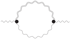
(a)(b)

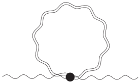
Figure 1: Feynman graphs with graviton (double) lines contributing to the photon two point function.

The calculation of the diagrams is straightforward, we used the symbolic manipulation program FORM [31] to deal with the large number of terms. The quadratically divergent contributions of the two graphs with improved cutoff (I) do not cancel each other

$$\Pi_{\mu\nu}^{\mathrm{I}(a)}(p) = \frac{i}{16\pi^{2}}\kappa^{2}\left(p^{2}\eta_{\mu\nu}-p_{\mu}p_{\nu}\right)\left(-2\Lambda^{2}-\frac{1}{6}p^{2}\left(\ln\left(\frac{\Lambda^{2}}{p^{2}}\right)+\frac{2}{3}\right)\right),$$ (11)

$$\Pi_{\mu\nu}^{\mathrm{I}(b)}(p) = \frac{i}{16\pi^{2}}\kappa^{2}\left(p^{2}\eta_{\mu\nu}-p_{\mu}p_{\nu}\right)\left(\phantom{2}\frac{3}{2}\Lambda^{2}\right).$$ (12)

In the naive cutoff (N) calculation using (36) there is a cancellation of the $\Lambda^{2}$ terms, the finite term do not match the previous one, and it is remarkable that the result is transverse without any subtractions

$$\Pi_{\mu\nu}^{\mathrm{N}(a)}(p) = \frac{i}{16\pi^{2}}\kappa^{2}\left(p^{2}\eta_{\mu\nu}-p_{\mu}p_{\nu}\right)\left(-\frac{3}{2}\Lambda^{2}-\frac{1}{6}p^{2}\ln\left(\frac{\Lambda^{2}}{p^{2}}\right)-\frac{7}{36}p^{2}\right),$$ (13)

$$\Pi_{\mu\nu}^{\mathrm{N}(b)}(p) = \frac{i}{16\pi^{2}}\kappa^{2}\left(p^{2}\eta_{\mu\nu}-p_{\mu}p_{\nu}\right)\left(\phantom{-}\frac{3}{2}\Lambda^{2}\right).$$ (14)

In dimensional regularization (DR) the space-time dimension is continued in all terms originating from the gauge and gravitational part, too (e.g. $\eta_{\mu}^{\mu}=d=4-2\epsilon$). The result (just as using the naive cutoff above) agrees with [15] (without the finite terms which are first given here)

$$\Pi_{\mu\nu}^{DR1(a)}(p) = \frac{i}{16\pi^{2}}\kappa^{2}\left(p^{2}\eta_{\mu\nu}-p_{\mu}p_{\nu}\right)\left(-\frac{1}{6}p^{2}\left(\frac{2}{\epsilon}+\ln\left(\frac{\mu^{2}}{p^{2}}\right)+\frac{1}{6}\right)\right),$$ (15)

$$\Pi_{\mu\nu}^{DR1(b)}(p) = 0,$$ (16)

where we have omitted the constants $-\gamma_{E}+\ln 4\pi$ beside $2/\epsilon$.

In what follows we present various “cutoff” results we arrived at using the technique of dimensional regularization based on different assumptions about the continuation of the dimension. Each result defines a different regularization scheme, and they are denoted by the superscript $DR1,\,DR2,\,DR3$ and the corresponding cutoff results by $\Lambda 1,\,\Lambda 2,\,\Lambda 3$ based on the extension of dimensional regularization.

Now with the help of the equations in the appendix (39), (40) and (41) we can define three cutoff results based on the dimensional regularization one. In the first case the dimension is modified in each terms where $d$ appears, also in the graviton propagator (5), though gravity is not a dynamical theory in $d=2$. Each graph is quadratically divergent, even $1/(\epsilon-1)^{2}$ type of singularities appear in single graphs, but they cancel in the sum of the graphs, like the $\frac{1}{\epsilon^{2}}$ terms in usual gauge theories (e.g. in QCD) at two loops.

$$\Pi_{\mu\nu}^{\mathrm{\Lambda 1}}(p)=\frac{i}{16\pi^{2}}\kappa^{2}\left(p^{2}\eta_{\mu\nu}-p_{\mu}p_{\nu}\right)\left(-\frac{1}{4}\Lambda^{2}-\frac{1}{6}p^{2}\left(\ln\left(\frac{\Lambda^{2}}{p^{2}}\right)-\frac{5}{6}\right)\right)$$ (17)

also quadratically divergent, but only the coefficient of the logarithmic term agrees with other results.

To find connection with existing, partially controversial literature, we have performed the calculation with weaker assumptions. First the term in the graviton propagator is set $\frac{1}{d-2}=\frac{1}{2}$ as is usually done in earlier results e.g. [27, 28]. The divergent part of the dimensional regularization result agrees with [15]. The contribution of the tadpole in Fig. 1b $\Pi^{\mathrm{DR2(b)}}$ vanishes, the sum is

$$\Pi_{\mu\nu}^{DR2}(p)=\frac{i}{16\pi^{2}}\kappa^{2}\left(p^{2}\eta_{\mu\nu}-p_{\mu}p_{\nu}\right)\left(-\frac{1}{6}p^{2}\left(\frac{2}{\epsilon}+\ln\left(\frac{\mu^{2}}{p^{2}}\right)+\frac{1}{6}\right)\right).$$ (18)

We can identify a cutoff result, Fig. 1b gives $\Pi_{\mu\nu}^{\mathrm{\Lambda 2(b)}}(p)\sim\frac{1}{2}\Lambda^{2}$, the only quadratically divergent term and

$$\Pi_{\mu\nu}^{\mathrm{\Lambda 2}}(p)=\frac{i}{16\pi^{2}}\kappa^{2}\left(p^{2}\eta_{\mu\nu}-p_{\mu}p_{\nu}\right)\left(\frac{1}{2}\Lambda^{2}-\frac{1}{6}p^{2}\left(\ln\left(\frac{\Lambda^{2}}{p^{2}}\right)-\frac{5}{6}\right)\right).$$ (19)

Notice that this result differs from (17) only in the value and the sign of the coefficient of the first term, the change originates from the different treatment of the graviton propagator.

The result of the improved momentum cutoff can be reproduced applying dimensional regularization with care. The improved cutoff method works in four physical dimensions and special rules have to be applied only at the evaluation of the last tensor integrals. It is equivalent to setting $d=4$ in the Einstein-Maxwell theory, e.g. both in the graviton propagator and in the trace of the metric tensor. Dimensional regularization is then applied at the last step evaluating the tensor and scalar momentum integrals. We have found that $\Pi_{\mu\nu}^{\mathrm{DR3(b)}}=0$ and

$$\Pi_{\mu\nu}^{DR3}(p)=\frac{i}{16\pi^{2}}\kappa^{2}\left(p^{2}\eta_{\mu\nu}-p_{\mu}p_{\nu}\right)\left(-\frac{1}{6}p^{2}\left(\frac{2}{\epsilon}+\ln\left(\frac{\mu^{2}}{p^{2}}\right)+\frac{5}{3}\right)\right).$$ (20)

The corresponding cutoff result diverges quadratically and agrees with the improved cutoff calculation (11,12)

$$\Pi_{\mu\nu}^{\mathrm{\Lambda 3}(a)}(p) = \frac{i}{16\pi^{2}}\kappa^{2}\left(p^{2}\eta_{\mu\nu}-p_{\mu}p_{\nu}\right)\left(-2\Lambda^{2}-\frac{1}{6}p^{2}\left(\ln\left(\frac{\Lambda^{2}}{p^{2}}\right)+\frac{2}{3}\right)\right),$$ (21)

$$\Pi_{\mu\nu}^{\mathrm{\Lambda 3}(b)}(p) = \frac{i}{16\pi^{2}}\kappa^{2}\left(p^{2}\eta_{\mu\nu}-p_{\mu}p_{\nu}\right)\left(\phantom{2}\frac{3}{2}\Lambda^{2}\right).$$ (22)

The quadratic divergences $\left(\Lambda^{2}\right)$ here are identified with the $d=2$ poles in the extension [48] of dimensional regularizations [51, 52]. There may appear an additional pole $1/(d-2)$ in the graviton propagator (5). It is coming from a non-physical point of the Einstein-Hilbert theory as this theory is not a dynamical one in $d=2$, the Lagrangian reduces to a trivial surface integral. In the first case, in (17) we apply continuous $d$ both in the propagator (5) and in the vertices during tracing. The second treatment sets $d=4$ in the propagator (as usually done in the literature) while using continuous $d$ during tracing the indices. This hybrid treatment looks not fully consistent as even in the loops one part of the theory feels the modified $d$ dimensions the other part not, e.g. feels fixed number of dimensions $d=4$ and gives (18). We prefer the third, conceptionally simple case, when the gravity algebra is performed in fixed $d=4$ and the rest of the calculation is done using the standard dimensional regularization technique. Moreover, the third result (21) and (22) agrees completely with the improved cutoff calculation case.

In principle a theory is completely defined via specifying the Lagrangian and the method of calculation e.g. fixing the regularization and the treatment of the divergent terms, though the physical quantities must be independent of the details of the regularization scheme. It is remarkable that the transverse structure of the photon propagator is not violated in any of the previous schemes and the logarithmic term is universal in the three cases and agrees with earlier results [15, 11]. The question is whether the $\Lambda^{2}$ terms contribute to the running of the gauge coupling, or have any other effects on measurable physical quantities.

3 Quadratic divergences and renormalization

In the previous section we have calculated the 1-loop radiative correction to the photon self energy from the effective theory of gravity in the simplest Maxwell-Einstein theory. We have found under various assumptions various quadratically divergent contributions (vanishing particularly using a naive momentum cutoff). The 1-loop corrections to the 2-point function generally modify the bare Lagrangian, the divergences have to be removed by the properly chosen counterterms via renormalization conditions.

Consider the QED action with the convention [32]

$$L_{0}=-\frac{1}{4e_{0}^{2}}F_{\mu\nu}F^{\mu\nu}+\bar{\Psi}iD_{\mu}\gamma^{\mu}\Psi,\qquad D_{\mu}=\partial_{\mu}+iA_{\mu}.$$ (23)

The divergences calculated from the interaction (1) gives the 1-loop effective action, here we focus only on the gravitational, divergent contributions

$$L=-\frac{1+a\kappa^{2}\Lambda^{2}}{4e_{0}^{2}}F_{\mu\nu}F^{\mu\nu}+a_{2}\ln\frac{\Lambda^{2}}{p^{2}}\left(D_{\mu}F^{\mu\nu}\right)^{2}+\left(\bar{\Psi}iD_{\mu}\gamma^{\mu}\Psi\right),$$ (24)

where $p^{2}$ is the Euclidean momentum at which the 2-point function was calculated. The question is whether should we interpret the coefficient of the usual kinetic term as a varying, i.e. running electric charge $\left(e^{2}(\Lambda)\simeq e_{0}^{2}\left(1-a\kappa^{2}\Lambda^{2}\right)\right)$? The answer is no, because of the necessary wavefunction and charge renormalization.

In quantum field theories the divergent terms have to be canceled by the counterterms. New dimension-six term must be added to match the $p^{2}\ln\left(\frac{\Lambda^{2}}{p^{2}}\right)$ term already shown in (24),

$$L_{\mathrm{\mathrm{ct}}}=\frac{\delta Z_{1}}{4e_{0}^{2}}F_{\mu\nu}F^{\mu\nu}+\delta Z_{2}\left(D_{\mu}F^{\mu\nu}\right)^{2}.$$ (25)

In principle there are three possible dimension-six counterterms $\left(D_{\mu}F^{\mu\nu}\right)^{2}$, $\left(D_{\mu}F_{\nu\rho}\right)^{2}$ and $F_{\mu}^{\nu}F_{\nu}^{\rho}F_{\rho}^{\mu}$. Only two of them are linearly independent up to total derivatives and it turns out that the first, the $\left(D_{\mu}F^{\mu\nu}\right)^{2}$ term can cancel all divergences [15]. The coefficient of the first term in (24) cannot be understood as defining a running coupling but it is compensated by a counterterm through a renormalization condition. It can be fixed either by the Coulomb potential or Thomson scattering at low energy identifying the usual electric charge as

$$\frac{e_{0}^{2}}{4\pi(1+a\kappa^{2}\Lambda^{2})}=\frac{e^{2}}{4\pi}\simeq\frac{1}{137}.$$ (26)

Thus the quadratically divergent correction defines the relation between the bare charge $e_{0}(\Lambda)$ in a theory with the physical cutoff $\Lambda$ and the physical charge effective at low energies. After fixing the parameters of the theory (e.g. by a measurement at low energy) and using $e$ to calculate the predictions of the model the cutoff dependence completely disappears from the physical charge [27, 32]. The role of the quadratic correction is to define the relation (26) this way renormalizing the bare coupling constant $e_{0}(\Lambda)$ ( and does not appear in the running of the physical charge).

Quadratic divergences are the main cause of the hierarchy problem and discussed with other regularization methods. In [33] the authors use Implicit Regularization, a general parametrization of the basic divergent integrals, which separates the divergences for a given problem in a process-independent way without referring to a specific regularization (see also the Appendix). They argue that their basic divergent integrals, thus the quadratic divergences can be absorbed in the renormalization constants without explicitly determining their value. Arbitrary parameters, such as the isolated quadratically divergent contribution to the Higgs mass can be fixed by additional (in the Higgs case: conformal) symmetry. Similar conclusion is reached in [34] using Wilsonian renormalization group (RG). They argued that the additive (they call it subtractive) and multiplicative renormalization procedure and the corresponding quadratic and logarithmic divergences can be treated independently. They show that quadratic divergences are the artifact of the regularization procedure and in the Wilsonian RG they are naturally subtracted and simply define position of the critical surface in the theory space. It is in complete agreement with our claim in (26) that the quadratic divergence disappears from the physical quantities. The fate of the logarithmic divergence could have been different.

The logarithmically divergent contribution on the other hand defines the renormalization of the higher dimensional operator $\left(D_{\mu}F^{\mu\nu}\right)^{2}$ and again not the running of the gauge coupling. After renormalization (at a point $p^{2}=\mu^{2}$) the logarithmic coefficient of the dim-6 term in (24) changes to $a_{2}\ln\frac{\Lambda^{2}}{p^{2}}-a_{2}\ln\frac{\Lambda^{2}}{\mu^{2}}=-a_{2}\ln\frac{p^{2}}{\mu^{2}}$ defining a would be running parameter. Furthermore note that this term can be removed [15, 26] by local field redefinition of $A_{\mu}$ up to higher dimensional operators

$$A_{\mu}\rightarrow A_{\mu}-c\nabla_{\nu}F_{\mu}^{\nu},$$ (27)

where $\nabla_{\mu}$ is the gravitational covariant derivative, as the new term is proportional to the tree level equation of motion

$$\nabla_{\mu}F^{\mu\nu}=0.$$ (28)

The logarithmic corrections were found in the first papers discussing the gravitational contributions by Deser et al. [11] using dimensional regularization and this way neglecting the quadratically divergent contribution spotted by [12]. Generally it can be shown, that all photon propagator corrections can be removed by appropriate field redefinition which are bilinear in $A_{\mu}$ even if they contain arbitrary number of derivatives, on-shell scattering processes are not influenced by the presence of such effective terms [35].

4 Corrections to the gauge coupling in Yang-Mills theories

We have discussed the simplest example including gravitational corrections in Chapter 2, but already Deser, Tsao and Nieuenhuizen [11] later Robinson and Wilczek [12] and many other authors performed their calculation in the Einstein-Yang-Mills system. Here we follow the presentation of [15] to show that after renormalization no meaningful running coupling can be defined even identifying quadratic divergences using cutoff regularization.

Consider the Einstein-Yang-Mills Lagrangian

$$S=\int\mathrm{d}^{4}x\sqrt{-g}\left[\frac{2}{\kappa^{2}}R-\frac{1}{2}g^{\mu\nu}g^{\alpha\beta}\mathrm{Tr}\left[F_{\mu\nu}F_{\alpha\beta}\right]\right],$$ (29)

where the field strength has a Yang-Mills index $F_{\mu\nu}=\partial_{\mu}A_{\nu}-\partial_{\nu}A_{\mu}-ig\left[A_{\mu},\>A_{\nu}\right]$ and $g$ is the Yang-Mills coupling.

In the Yang-Mills theory the bare gluon three-point functions get modified by gravity, too. Beside the corrections to the gluon two point functions, which are order $\kappa^{2}$ and are the same as presented in Chapter 2 see (13) and (14) and Figure 1, there are contributions to the gluon three-point functions at the $g\kappa^{2}$ order.

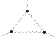
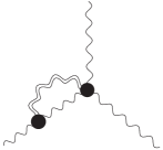
(c) (d) (e)

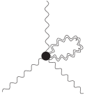
Figure 2: Feynman graphs with graviton (double) lines contributing to the gluon three point function.

There are new vertices with three selfinteracting gluon with extra one- and two-graviton legs. The three gluon-one graviton vertex is

$$V_{gggG}(k_{1\mu}^{(a)},k_{2\nu}^{(b)},k_{3\rho}^{(c)},\alpha\beta) \!=\! -\!ig\kappa f^{abc}\left[P^{\alpha\beta,\mu\nu}\left(k_{1}-k_{2}\right)^{\rho}+\eta^{\alpha\beta}\left(\eta^{\rho\alpha}\left(k_{1}-k_{2}\right)^{\beta}+\eta^{\rho\alpha}\left(k_{1}-k_{2}\right)^{\beta}\right)+\right.$$ (30)

$$\!\left.+\mathrm{cycl.perm.}\left\{(\mu,k_{1}),(\nu,k_{2}),(\rho,k_{3})\right\}\right],$$

where $f^{abc}$ is the Yang-Mills structure constant. The three gluon-two graviton vertex is again rather complicated and lengthy

$$V_{gggGG}(k_{1\mu}^{(a)},k_{2\nu}^{(b)},k_{3\rho}^{(c)},\alpha\beta,\gamma\delta) \!=\! -ig\kappa^{2}f^{abc}\left[\left(k_{1}-k_{2}\right)^{\rho}\left(I^{\mu\nu,\alpha\gamma}\eta^{\delta\beta}+I^{\mu\nu,\alpha\delta}\eta^{\gamma\beta}+\left\{{}^{(\mu\nu)\longleftrightarrow(\alpha\beta)}\right\}\right.\right.$$ (31)

$$-\left.\frac{1}{2}\left(\eta^{\alpha\beta}I^{\mu\nu,\gamma\delta}+\eta^{\gamma\delta}I^{\mu u,\alpha\beta}\right)-\eta^{\mu\nu}P^{\alpha\beta,\gamma\delta}\right)$$

$$+\left(2\eta^{\mu\nu}P^{\gamma\delta,\alpha\beta}+I^{\mu\nu,\gamma\delta}\right)\left(k_{1}-k_{2}\right)^{\rho}+\left\{{}^{(\alpha)\longleftrightarrow(\beta)}\right\}$$

$$\!\left.\left\{{}^{(\gamma\delta)\longleftrightarrow(\alpha\beta)}\right\}+\mathrm{cycl.perm.}\left\{(\mu,k_{1}),(\nu,k_{2}),(\rho,k_{3})\right\}\right].$$

With these vertices there are three graphs contributing to the gluon three-point function at one-loop, Fig.2. The external gluons are labeled as in the vertices $\left\{(\mu,k_{1}),(\nu,k_{2}),(\rho,k_{3})\right\}$ and the the 3-point function contributions must be symmetrized in these index-pairs. The graph $(c)$ is only logarithmically divergent

$$G_{3}^{(c)}\sim\frac{1}{16\pi^{2}}g\kappa^{2}f^{abc}\log\Lambda^{2}F_{3}^{\mu\nu\rho}\left(k_{1}^{\mu},k_{2}^{\nu},k_{3}^{\rho}\right),$$ (32)

where the lengthy $F_{3}^{\mu\nu\rho}$ function scales with the third power of momenta. The graphs (d) and (e) are similar to (a) and (b) only with the exception of an additional gluon leg starting from the main vertex. Graph (d) has similar logarithmic correction as (32) and a quadratic divergence, while in (e) the divergence is purely quadratic.

$$G_{3}^{(d)} \simeq \phantom{{\}}}\frac{1}{16\pi^{2}}g\kappa^{2}f^{abc}\frac{3}{2}\left(\eta^{\mu\nu}\left(k_{1}-k_{2}\right)^{\rho}+\mathrm{symmetrized}\right)\Lambda^{2}+\mathrm{log\>terms},$$ (33)

$$G_{3}^{(e)} \simeq -\frac{1}{16\pi^{2}}g\kappa^{2}f^{abc}\frac{3}{2}\left(\eta^{\mu\nu}\left(k_{1}-k_{2}\right)^{\rho}+\mathrm{symmetrized}\right)\Lambda^{2}.$$ (34)

The sum of the quadratic contributions from graphs (d) and (e) exactly cancel just as for the two point functions in Fig. 1. The remaining logarithmic divergence surprisingly can be canceled by only the second term in (25).

$$L_{c.t.}\supset\frac{1}{16\pi^{2}}\frac{1}{6}\kappa^{2}\log\frac{\Lambda^{2}}{\mu^{2}}\left(D_{\mu}F^{\mu\nu}\right),$$ (35)

where $\mu$ is the renormalization scale in agreement with the result of [11] and later works. We emphasize that the counterterm in (35) corrects a higher dimensional operator, and the contribution can be removed by a non-linear field redefinitions of the gauge field (27) as discussed in Chapter 3 and does not lead to a change in the running of physical parameters.

5 Conclusion

We have calculated and presented in this chapter the gravitational corrections to gauge theories in the framework of effective field theories. The study was motivated by the various, sometime controversial results in the literature. Our method and the presented results were capable of identifying quadratically divergent contributions to the photon and generalized gluon two and three point functions, thanks to the gauge invariant construction. In the first, QED part, to test our calculation we defined the cutoff dependence employing (39), (40) and dimensional regularization with various assumptions about treating the number of dimensions $d$. We observed that the 1-loop gravity corrections to the two point function in all but one cases contain $\Lambda^{2}$ divergence with the exception of the naive momentum cutoff which violates gauge symmetries usually. Here all the corrections are transverse. The logarithmic term universally agrees with the literature starting from Deser et al. [11]. Then we presented the corrections in a more general Yang-Mills theory. We found that the logarithmically divergent terms contribute to the dimension-6 terms and can be removed by local field redefinitions this way do not affecting the running of the gauge coupling. $\Lambda^{2}$ corrections to the QED or Yang-Mills effective actions are absent using a naive cutoff regularizations and are present with more sophisticated methods, but those are proved to be non-physical.

The quadratically divergent corrections to the photon or gluon self-energy do not lead to the modification of the running of the gauge coupling. Robinson and Wilczek claimed that the $-a\kappa^{2}\Lambda^{2}$ correction could turn the beta function negative and make the Einstein-Maxwell and Einstein-Yang-Mills theory asymptotically free. This statement and the calculation was criticized in the literature. We showed in this chapter using explicit cutoff calculation that $\Lambda^{2}$ corrections may appear in the 2-point function, but those will define the renormalization connection between the cutoff dependent bare coupling and the physical coupling (26) and do not lead to a running coupling. This conclusion is in complete agreement with other results concerning quadratic divergences [27, 33, 34]. Indeed the $\Lambda^{2}$ correction can be absorbed into the physical charge and does not appear in physical processes. Donoghue et al. argue in [27] that an universal, i.e. process independent running coupling constant cannot be defined in the effective theory of gravity independently of the applied regularization. They demonstrate that because of the crossing symmetry in theories (except the $\lambda\Phi^{4}$) even the sign of the would be quadratic running is ambiguous and a running coupling would be process dependent, thus not useful. Generally the logarithmically divergent corrections could define the renormalization of higher dimensional operators. It turns out that even these logarithmic correction can be removed by appropriate field redefinitions and do not contribute to on-shell scattering processes. We note that the authors in [28] showed using their 4-dimensional implicit regularization method that the quadratic terms are coming from ambiguous surface terms, discussed in more details in [30, 43], and as such are non-physical. Interestingly those surface terms vanish if we evaluate them with our improved cutoff [36].

Finally we point out that we have found gravity corrections to the two and three-point functions in gauge theories. Using a momentum cutoff the quadratically divergent contributions define the renormalization of the bare charge and thus using the physical charge the $\Lambda^{2}$ corrections do not appear in physical processes. On the other hand logarithmic corrections are universal but merely define the renormalization of a dimension-6 term in the Lagrangian, which term can be eliminated by local field redefinition. We conclude that gravity corrections do not lead to the modification of the usual running of gauge coupling and cannot point towards asymptotic freedom in the case of gauge theories.

Appendix: Improved momentum cutoff

In this appendix we introduce the novel regularization of gauge theories, proposed in [30] and discussed with broader outlook on the literature in [36]. It is based on 4 dimensional momentum cutoff to evaluate 1-loop divergent integrals. The idea was to construct a cutoff regularization which does not brake gauge symmetries and the necessary shift of the loop-momentum is allowed as no surface terms are generated. The loop calculation starts with Wick rotation, Feynman-parametrization and loop-momentum shift. Only the treatment of free Lorentz indices under divergent integrals should be changed compared to the naive cutoff calculation.

We start with the observation that the contraction with $\eta_{\mu\nu}$ (tracing) does not necessarily commute with loop-integration in divergent cases. Therefore the substitution of

$$k_{\mu}k_{\nu}\rightarrow\frac{1}{4}\eta_{\mu\nu}k^{2}$$ (36)

is not valid under divergent integrals, where $k$ is the loop-momentum. The usual factor $1/4$ is the result of tracing both sides under the loop integral, e.g. changing the order of tracing and the integration. In the new approach the integrals with free Lorentz indices are defined using physical consistency conditions, such as gauge invariance or freedom of momentum routing. Based on the diagrammatic proof of gauge invariance it can be shown that the two conditions are related and both are in connection with the requirement of vanishing surface terms. It was proposed in [30] that instead of (36) the general identification of the cutoff regulated integrals in gauge theories

$$\int_{\Lambda\>reg}d^{4}l_{E}\frac{l_{E\mu}l_{E\nu}}{\left(l_{E}^{2}+m^{2}\right)^{n+1}}=\frac{1}{2n}\eta_{\mu\nu}\int_{\Lambda\>reg}d^{4}l_{E}\frac{1}{\left(l_{E}^{2}+m^{2}\right)^{n}},\ \ \ \ \ n=1,2,...$$ (37)

will satisfy the Ward-Takahashi identities and gauge invariance at 1-loop ($l{}_{E}$ is the shifted Euclidean loop-momentum). In case of divergent integrals it differs from (36), for non-divergent cases both substitutions give the same results at ${\cal O}(1/\Lambda^{2})$ (the difference is a vanishing surface term). It is shown in [30] that this definition is robust in gauge theories, differently organized calculations of the 1-loop functions agree with each other using (37) and disagree using (36). For four free indices the gauge invariance dictates ($n=2,3,...$)

$$\int_{\Lambda\>reg}d^{4}l_{E}\frac{l_{E\alpha}l_{E\beta}l_{E\mu}l_{E\rho}}{\left(l_{E}^{2}+m^{2}\right)^{n+1}}=\frac{1}{4n(n-1)}\int_{\Lambda\>reg}d^{4}l_{E}\frac{\eta_{\alpha\beta}\eta_{\mu\rho}+\eta_{\alpha\mu}\eta_{\beta\rho}+\eta_{\alpha\rho}\eta_{\beta\mu}}{\left(l_{E}^{2}+m^{2}\right)^{n-1}}.$$ (38)

For 6 and more free indices appropriate rules can be derived (or (37) can be used recursively for each allowed pair). Finally the scalar integrals are evaluated with a simple Euclidean momentum cutoff. The method was successfully applied to an effective model to estimate oblique corrections [37].

There are similar attempts to define a regularization that respects the original gauge and Lorentz symmetries of the Lagrangian but work in four spacetime dimensions usually with a cutoff [38, 39]. Some methods can separate the divergences of the theories and does not rely on a physical cutoff [40, 41, 42] or even could be independent of it [44]. For further literature see references in [30].

Under this modified cutoff regularization the terms with numerators proportional to the loop momentum are all defined by the possible tensor structures. Odd number of $l_{E}$’s give zero as usual, but the integral of even number of $l_{E}$’s is defined by (37), (38) and similarly for more indices, this guarantees that the symmetries are not violated. The calculation is performed in 4 dimensions, the finite terms are equivalent with the results of dimensional regularization. The method identifies quadratic divergences while gauge and Lorentz symmetries are respected. We stress that the method treats differently momenta with free ($k_{\mu}k_{\nu}$) and contracted Lorentz indices ($k^{2}$), the order of tracing and performing the regulated integral cannot be changed similarly to dimensional regularization. The famous triangle anomaly can be unambiguously defined and presented in [45] see also [46], [47].

However even using dimensional regularization one is able to define cutoff results in agreement with the present method. In dimensional regularization singularities are identified as $1/\epsilon$ poles, power counting shows that these are the logarithmic divergences of the theory. Naively quadratic divergences are set to zero in the process, but already Veltman noticed [48] that these divergences can be identified by calculating the poles in $d=2$ $(\epsilon=1)$. Careful calculation of the Veltman-Passarino 1-loop functions in dimensional regularization and with 4-momentum cutoff leads to the following identifications [30, 49, 50]

$$4\pi\mu^{2}\left(\frac{1}{\epsilon-1}+1\right) = \Lambda^{2},$$ (39)

$$\frac{1}{\epsilon}-\gamma_{E}+\ln\left(4\pi\mu^{2}\right)+1 = \ln\Lambda^{2}.$$ (40)

The finite terms are unambiguously defined

$$f_{{\rm finite}}=\lim_{\epsilon\rightarrow 0}\left[f(\epsilon)-R(0)\left(\frac{1}{\epsilon}-\gamma_{E}+\ln 4\pi+1\right)-R(1)\left(\frac{1}{\epsilon-1}+1\right)\right],$$ (41)

where $R(0)$,   $R(1)$ are the residues of the poles at $\epsilon=0,\,1$ respectively. Using (39), (40) and (41) at 1-loop the results of the improved cutoff can be reproduced using dimensional regularization without any ambiguous subtraction.

The loop integrals are calculated as follows. First the loop momentum ($k$) integral is Wick rotated (to $k_{E}$), with Feynman parameter(s) the denominators are combined, then the order of Feynman parameter and the momentum integrals are changed. After that the loop momentum ($k_{E}\rightarrow l_{E}$) is shifted to have a spherically symmetric denominator.

Finally we present two divergent integrals calculated by the new regularization. $\Delta$ can be any loop momentum independent expression depending on the Feynman $x$ parameter, external momenta, masses, e.g. $\Delta(x,q_{i},m).$ The integration is understood for Euclidean momenta with absolute value below the $\Lambda$ cutoff $\left(|l_{E}|\leq\Lambda\right)$.

The integral (42) is just given for comparison, it is calculated with a simple momentum cutoff. In (43) with the standard (36) substitution one would get a constant $-\frac{3}{2}$ instead of $-1$ [30].

$$\int_{\Lambda\,reg}\frac{d^{4}l_{E}}{i(2\pi)^{4}}\frac{1}{\left(l_{E}^{2}+\Delta^{2}\right)^{2}} \!\!=\!\! \frac{1}{(4\pi)^{2}}\left(\ln\left(\frac{\Lambda^{2}+\Delta^{2}}{\Delta^{2}}\right)+\frac{\Delta^{2}}{\Lambda^{2}+\Delta^{2}}-1\right).$$ (42)

$$\int_{\Lambda\,reg}\frac{d^{4}k}{i(2\pi)^{4}}\frac{l_{E\mu}l_{E\nu}}{\left(l_{E}^{2}+\Delta^{2}\right)^{3}} \!\!=\!\! \frac{1}{(4\pi)^{2}}\frac{g_{\mu\nu}}{4}\left(\ln\left(\frac{\Lambda^{2}+\Delta^{2}}{\Delta^{2}}\right)+\frac{\Delta^{2}}{\Lambda^{2}+\Delta^{2}}-1\right).$$ (43)

References

- [1] B. P. Abbott et al. [LIGO Scientific and Virgo Collaborations], Phys. Rev. Lett. 116 (2016) no.6, 061102.
- [2] G. ’t Hooft and M. J. G. Veltman, Annales Poincare Phys. Theor. A 20 (1974) 69.
- [3] J. F. Donoghue, Phys. Rev. D 50 (1994) 3874.
- [4] J. F. Donoghue, AIP Conf. Proc. 1483 (2012) 73.
- [5] C. P. Burgess, Living Rev. Rel. 7 (2004) 5.
- [6] G. Aad et al. [ATLAS Collaboration], Phys. Lett. B 716 (2012) 1.
- [7] S. Chatrchyan et al. [CMS Collaboration], Phys. Lett. B 716 (2012) 30.
- [8] G. Degrassi, S. Di Vita, J. Elias-Miro, J. R. Espinosa, G. F. Giudice, G. Isidori and A. Strumia, JHEP 1208 (2012) 098.
- [9] F. Bezrukov, M. Y. Kalmykov, B. A. Kniehl and M. Shaposhnikov, JHEP 1210 (2012) 140.
- [10] D. Buttazzo, G. Degrassi, P. P. Giardino, G. F. Giudice, F. Sala, A. Salvio and A. Strumia, arXiv:1307.3536 [hep-ph].
- [11] S. Deser, H. -S. Tsao and P. van Nieuwenhuizen, Phys. Rev. D 10 (1974) 3337.
- [12] S. P. Robinson and F. Wilczek, Phys. Rev. Lett. 96 (2006) 231601.
- [13] A. R. Pietrykowski, Phys. Rev. Lett. 98 (2007) 061801.
- [14] D. J. Toms, Phys. Rev. D 76 (2007) 045015.
- [15] D. Ebert, J. Plefka and A. Rodigast, Phys. Lett. B 660 (2008) 579.
- [16] D. J. Toms, Nature 468 (2010) 56.
- [17] Y. Tang and Y. -L. Wu, Commun. Theor. Phys. 57 (2012) 629.
- [18] A. R. Pietrykowski, Phys. Rev. D 87 (2013) 024026.
- [19] H. -J. He, X. -F. Wang and Z. -Z. Xianyu, Phys. Rev. D 83 (2011) 125014.
- [20] N. K. Nielsen, Annals Phys. 327 (2012) 861.
- [21] S. Weinberg, in General Relativity: An Einstein Centenary Survey, ed. by S. Hawking and W. Israel, Cambridge UNiversity press, 1979, p.790
- [22] M. Niedermaier and M. Reuter, Living Rev. Rel. 9 (2006) 5.
- [23] J. -E. Daum, U. Harst and M. Reuter, JHEP 1001 (2010) 084.
- [24] S. Folkerts, D. F. Litim and J. M. Pawlowski, Phys. Lett. B 709 (2012) 234.
- [25] G. Narain and R. Anishetty, JHEP 1307 (2013) 106.
- [26] J. Ellis and N. E. Mavromatos, Phys. Lett. B 711 (2012) 139.
- [27] M. M. Anber, J. F. Donoghue and M. El-Houssieny, Phys. Rev. D 83 (2011) 124003.
- [28] J. C. C. Felipe, L. C. T. Brito, M. Sampaio and M. C. Nemes, Phys. Lett. B 700 (2011).
- [29] G. Cynolter and E. Lendvai, Mod. Phys. Lett. A 29 (2014) 1450024.
- [30] G. Cynolter and E. Lendvai, Central Eur.J.Phys. 9 (2011) 1237.
- [31] J. A. M. Vermaseren, “New features of FORM,” math-ph/0010025.
- [32] M. M. Anber and J. F. Donoghue, Phys. Rev. D 85 (2012) 104016.
- [33] A. L. Cherchiglia, A. R. Vieira, B. Hiller, A. P. Baêta Scarpelli and M. Sampaio, Annals Phys. 351 (2014) 751 doi:10.1016/j.aop.2014.10.002
- [34] H. Aoki and S. Iso, Phys. Rev. D 86 (2012) 013001 doi:10.1103/PhysRevD.86.013001
- [35] A. A. Tseytlin, Phys. Lett. B 176 (1986) 92.
- [36] G. Cynolter and E. Lendvai, in Gauge Theories and Differential Geometry, (editor Lance Bailey), pp. 199-218 ISBN: 978-1-63483-546-6, arXiv:1509.07407 [hep-ph].
- [37] G. Cynolter, E. Lendvai and G. Pócsik, Mod. Phys. Lett. A 24 (2009) 2331.
- [38] Y. Gu, J. Phys. A 39 (2006) 13575.
- [39] Y. L. Wu, Int. J. Mod. Phys. A 18 (2003) 5363.
- [40] O. A. Battistel and M. C. Nemes, Phys. Rev. D 59 (1999) 055010.
- [41] S. Arnone, T. R. Morris and O. J. Rosten, Eur. Phys. J. C 50 (2007) 467.
- [42] F. del Aguila and M. Perez-Victoria, Acta Phys. Polon. B 29 (1998) 2857.
- [43] A. R. Vieira, A. L. Cherchiglia and M. Sampaio, Phys. Rev. D 93 (2016) no.2, 025029 doi:10.1103/PhysRevD.93.025029
- [44] R. Pittau, JHEP 1211 (2012) 151.
- [45] G. Cynolter and E. Lendvai, Mod. Phys. Lett. A 26 (2011) 1537.
- [46] B. K. El-Menoufi and G. A. White, arXiv:1505.01754 [hep-th].
- [47] A. C. D. Viglioni, A. L. Cherchiglia, A. R. Vieira, B. Hiller and M. Sampaio, arXiv:1606.01772 [hep-th].
- [48] M.J.G Veltman, Acta Phys. Polon. B12: (1981) 437.
- [49] K. Hagiwara, S. Ishihara, R. Szalapski and D. Zeppenfeld, Phys. Rev. D 48 (1993) 2182.
- [50] M. Harada and K. Yamawaki, Phys. Rev. D 64, 014023 (2001).
- [51] G. ’t Hooft and M. J. G. Veltman, Nucl. Phys. B 44 (1972) 189.
- [52] G. Leibbrandt, Rev. Mod. Phys. 47 (1975) 849.