Smeared Coulomb potential orbitals for the electron-nucleus mean field configuration interaction method

Patrick Cassam-ChenaΓ― cassam@unice.fr    Gilles Lebeau [
Abstract

We propose to use the eigenfunctions of a one-electron model Hamiltonian to perform electron-nucleus mean field configuration interaction (EN-MFCI) calculations. The potential energy of our model Hamiltonian corresponds to the Coulomb potential of an infinite wire with charge $Z$ distributed according to a Gaussian function. The time independent SchrΓΆdingerΒ equation for this Hamiltonian is solved perturbationally in the limit of small amplitude vibration (Gaussian function width close to zero).

University of Nice Sophia Antipolis]UniversitΓ© CΓ΄te d’Azur, LJAD, UMR 7351, 06100 Nice, France

1 Introduction

This paper is dedicated to Prof. Graham Chandler, whose famous β€œMclean and Chandler basis sets” have proved extremely useful to the quantum chemistry community. Some twenty years ago, we optimized Gaussian basis sets for molecular fragments together with D. Jayatilaka and G. S. Chandler 1. However, this endeavour was suspended due to technical difficulties raised by electronegative atoms. In the present article, we come back to, perhaps, a more original approach to basis functions, where the latter are not selected on the ground of their technical advantages, as was the case initially for Gaussian-type orbitals (GTO) 2, but because they are eigenfunctions of a model Hamiltonian and therefore have some physical relevance. It is hoped that this property can be taken advantage of in basis set truncation.

The model Hamiltonian we will consider is a generalization of the hydrogenoid atom Coulomb Hamiltonian. So, our new orbitals will be part of the exponential-type orbitals (ETO) 3 family, as the hydrogenoid atom eigenfunctions, which constitute an asymptotic limit. Slater-type orbitals (STO) 4, 5 is another type of ETO related to hydrogenoid orbitals (HO): they can be seen as β€œuncontracted” HO, that is to say, as HO with the Laguerre polynomial prefactor replaced by a simple monomial one. In contrast to GTO, the difficulty of computing multicenter integrals with STO has led to the introduction of more ETO family members such as Bessel-type orbitals (BTO) 6 or Coulomb-Sturmian orbitals (CSO) 7. The techniques developed for the latter 8, 9, 10 will be equally relevant for integrals involving our deformed hydrogenoid orbitals (DHO).

It is our take that DHO will be particularly useful for the recently developed electron-nucleus mean field configuration interaction (EN-MFCI) method 11. The EN-MFCI method affords one to obtain in a single calculation, the electronic and vibrational energy levels of a molecule, without making the β€œBorn-Oppenheimer” (BO) approximation 11, 12. In contrast, the traditional methods of Quantum Chemistry are set in the frame of this approximation. They describe electronic clouds of fixed nuclear configurations and make use of orbital basis sets centered on nuclear positions. The latter basis sets are not appropriate for EN-MFCI calculations and their discrepancies have been bypassed so far, only by adding off-centered orbitals. However, these additional functions introduce linear dependencies with the initial orbitals and span virtual molecular orbitals of little relevance for the description of low energy wave functions of the molecule. So, it appears important to develop new orbital basis sets for the EN-MFCI method, able to describe the electron cloud of oscillating nuclei in a molecular system.

We propose to use the eigenfunctions of a one-electron model Hamiltonian:
$H=-\frac{\vartriangle}{2\mu}+V(\vec{r})$, with a potential of the form:

$$V(\vec{r})=-Z\sqrt{\frac{a}{\pi}}\int\limits_{-\infty}^{+\infty}\frac{exp[-az_{0}^{2}]}{\Arrowvert\vec{r}-\vec{r_{z_{0}}}\Arrowvert}dz_{0},$$ (1)

where, $Z\in\mathbb{N}$, $a\in\mathbb{R}^{+}$, $\vec{r}=(x,y,z)$ and $\vec{r_{z_{0}}}=(0,0,z_{0})$ in Cartesian coordinates. When $\vec{r}$ is expressed in cylindrical coordinates, $\vec{r}=(\rho,\phi,z)$, the potential depends only upon $\rho$ and $z$,

$$V(\rho,z)=-Z\sqrt{\frac{a}{\pi}}\int\limits_{-\infty}^{+\infty}\frac{exp[-az_{0}^{2}]}{\sqrt{\rho^{2}+(z-z_{0})^{2}}}dz_{0}.$$ (2)

This potential corresponds to the Coulomb potential of an infinite wire with charge $Z$ distributed according to a Gaussian function. In the limiting case of a Gaussian function sharply peaking at the origin ($a\rightarrow+\infty$, Dirac distribution limit), the system will tends towards a point-charge Z concentrated at the origin and the hydrogenoid atom eigenfunctions will be recovered.
However, by taking a Gaussian width parameter of the order of magnitude of a nucleus vibration amplitude, we will get basis functions corresponding to a Coulomb potential convoluted by a nuclear, vibrational, harmonic motion, that we may think particularly appropriate for EN-MFCI calculations.
Unfortunately, the SchrΓΆdingerΒ equation for this potential is hard to solve because the whole $z$-axis is singular. So, we will restrict ourselves to the $a\rightarrow\infty$ asymptotic limit, and expand the potential $V(\rho,z)$ as

$\displaystyle V(\rho,z)=\frac{-Z\sqrt{a}}{\pi}\int\limits_{0}^{+\infty}\frac{d\lambda}{\sqrt{\lambda}}\int\limits_{-\infty}^{+\infty}dz_{0}\ exp[-az_{0}^{2}-\lambda(\rho^{2}+(z-z_{0})^{2})]$
$\displaystyle=-Z\sqrt{\frac{a}{\pi}}\int\limits_{0}^{+\infty}\frac{d\lambda}{\sqrt{\lambda(a+\lambda)}}exp[-\lambda(\rho^{2}+z^{2})]exp[\frac{\lambda^{2}}{a+\lambda}z^{2}]$
$\displaystyle=\frac{-Z}{\sqrt{\pi}}\int\limits_{0}^{+\infty}d\lambda\left(\frac{1}{\sqrt{\lambda}}+\frac{-\frac{\lambda}{2}+z^{2}\lambda^{2}}{\sqrt{\lambda}a}+\frac{\lambda^{3/2}\left(3-12z^{2}\lambda+4z^{4}\lambda^{2}\right)}{8a^{2}}+\frac{\lambda^{5/2}\left(-15+90z^{2}\lambda-60z^{4}\lambda^{2}+8z^{6}\lambda^{3}\right)}{48a^{3}}+o\left(\frac{1}{a}\right)^{\frac{7}{2}}\right)exp[-\lambda(\rho^{2}+z^{2})]$

Swaping the limits and setting $r=\sqrt{\rho^{2}+z^{2}}$, ρ=rΓ—s​i​n​(ΞΈ)πœŒπ‘Ÿπ‘ π‘–π‘›πœƒ\rho=r\times sin(\theta), z=rΓ—c​o​s​(ΞΈ)π‘§π‘Ÿπ‘π‘œπ‘ πœƒz=r\times cos(\theta), with $\theta\in\left[0,\pi\right]$, the potential becomes

V​(r,ΞΈ)=βˆ’Zr+(1βˆ’3​c​o​s​(ΞΈ)2)​Z4​r3​aβˆ’3​((3βˆ’30​c​o​s​(ΞΈ)2+35​c​o​s​(ΞΈ)4)​Z)32​r5​a2+15​(5βˆ’105​c​o​s​(ΞΈ)2+315​c​o​s​(ΞΈ)4βˆ’231​c​o​s​(ΞΈ)6)​Z128​r7​a3+O​[1a]4,π‘‰π‘Ÿπœƒπ‘π‘Ÿ13π‘π‘œπ‘ superscriptπœƒ2𝑍4superscriptπ‘Ÿ3π‘Ž3330π‘π‘œπ‘ superscriptπœƒ235π‘π‘œπ‘ superscriptπœƒ4𝑍32superscriptπ‘Ÿ5superscriptπ‘Ž2155105π‘π‘œπ‘ superscriptπœƒ2315π‘π‘œπ‘ superscriptπœƒ4231π‘π‘œπ‘ superscriptπœƒ6𝑍128superscriptπ‘Ÿ7superscriptπ‘Ž3𝑂superscriptdelimited-[]1π‘Ž4\displaystyle V(r,\theta)=-\frac{Z}{r}+\frac{\left(1-3cos(\theta)^{2}\right)Z}{4r^{3}a}-\frac{3\left(\left(3-30cos(\theta)^{2}+35cos(\theta)^{4}\right)Z\right)}{32r^{5}a^{2}}+\frac{15\left(5-105cos(\theta)^{2}+315cos(\theta)^{4}-231cos(\theta)^{6}\right)Z}{128r^{7}a^{3}}+O\left[\frac{1}{a}\right]^{4},

where we recognize the hydrogenoid atom potential in the zeroth-order term.

$$V^{(0)}(r,\theta)=-\frac{Z}{r}.$$ (5)

Now, at any order, the singularity is located at the single point $r=0$. In the following, we will only consider the $V(r,\theta)$ potential truncated at first order,

V1​(r,ΞΈ):=βˆ’Zr+(1βˆ’3​c​o​s​(ΞΈ)2)​Z4​r3​a.assignsubscript𝑉1π‘Ÿπœƒπ‘π‘Ÿ13π‘π‘œπ‘ superscriptπœƒ2𝑍4superscriptπ‘Ÿ3π‘ŽV_{1}(r,\theta):=-\frac{Z}{r}+\frac{\left(1-3cos(\theta)^{2}\right)Z}{4r^{3}a}. (6)

Since this potential is not bounded from below, we will just apply Rayleigh-SchrΓΆdingerΒ perturbation theory to first order, to get corrections with respect to the hydrogenoid atom eigenstates.

2 Perturbationally corrected eigenstates

So, we consider the following Hamiltonian in spherical coordinates and atomic units

H=βˆ’12​μ​(1r2β€‹βˆ‚βˆ‚r​r2β€‹βˆ‚βˆ‚r+1r2​s​i​n​(ΞΈ)β€‹βˆ‚βˆ‚ΞΈβ€‹s​i​n​(ΞΈ)β€‹βˆ‚βˆ‚ΞΈ+1r2​s​i​n​(ΞΈ)2β€‹βˆ‚2βˆ‚Ο•2)+V1​(r,ΞΈ),𝐻12πœ‡1superscriptπ‘Ÿ2π‘Ÿsuperscriptπ‘Ÿ2π‘Ÿ1superscriptπ‘Ÿ2π‘ π‘–π‘›πœƒπœƒπ‘ π‘–π‘›πœƒπœƒ1superscriptπ‘Ÿ2𝑠𝑖𝑛superscriptπœƒ2superscript2superscriptitalic-Ο•2subscript𝑉1π‘ŸπœƒH=\frac{-1}{2\mu}\left(\frac{1}{r^{2}}\frac{\partial}{\partial r}r^{2}\frac{\partial}{\partial r}+\frac{1}{r^{2}sin(\theta)}\frac{\partial}{\partial\theta}sin(\theta)\frac{\partial}{\partial\theta}+\frac{1}{r^{2}sin(\theta)^{2}}\frac{\partial^{2}}{\partial\phi^{2}}\right)+V_{1}(r,\theta), (7)

defined on the Hilbert space of square integrable functions whose scalar product is expressed as,

⟨ψ1|ψ2⟩:=∫0+∞r2​𝑑rβ€‹βˆ«0Ο€s​i​n​(ΞΈ)β€‹π‘‘ΞΈβ€‹βˆ«02β€‹Ο€π‘‘Ο•β€‹Οˆ1βˆ—β€‹(r,ΞΈ,Ο•)β€‹Οˆ2​(r,ΞΈ,Ο•).assigninner-productsubscriptπœ“1subscriptπœ“2superscriptsubscript0superscriptπ‘Ÿ2differential-dπ‘Ÿsuperscriptsubscript0πœ‹π‘ π‘–π‘›πœƒdifferential-dπœƒsuperscriptsubscript02πœ‹differential-ditalic-Ο•superscriptsubscriptπœ“1π‘Ÿπœƒitalic-Ο•subscriptπœ“2π‘Ÿπœƒitalic-Ο•\langle\psi_{1}|\psi_{2}\rangle:=\int\limits_{0}^{+\infty}r^{2}dr\int\limits_{0}^{\pi}sin(\theta)d\theta\int\limits_{0}^{2\pi}d\phi\ \psi_{1}^{*}(r,\theta,\phi)\psi_{2}(r,\theta,\phi). (8)

A Galerkin-type approach similar to the one proposed in 13, with spherical harmonics in place of Chebychev basis functions could be considered to solve its eigenvalue problem. However, it is more practical to approach the eigenstates perturbationally, starting from the well-known solutions of time-independent SchrΓΆdingerΒ equation for the hydrogenoid atom,

$$\psi^{(0)}_{n,l,m}(r,\theta,\phi)=R_{n,l}(r)Y_{l,m}(\theta,\phi)$$ (9)

with

$$R_{n,l}(r)=\left(\frac{2\mu Z}{n}\right)^{\frac{3}{2}}\sqrt{\frac{(n-l-1)!}{2n[(n+l)!]}}exp\left(-\frac{\mu Zr}{n}\right)\left(\frac{2\mu Zr}{n}\right)^{l}L_{n-l-1}^{2l+1}\left(\frac{2\mu Zr}{n}\right),$$ (10)

where $L_{n-l-1}^{2l+1}(x)$ denotes the generalized Laguerre polynomials, and $Y_{l,m}(\theta,\phi)$ the spherical harmonics. We note that the perturbation operator,

V(1)​(r,ΞΈ):=(1a)​(1βˆ’3​c​o​s​(ΞΈ)2)​Z4​r3.assignsuperscript𝑉1π‘Ÿπœƒ1π‘Ž13π‘π‘œπ‘ superscriptπœƒ2𝑍4superscriptπ‘Ÿ3V^{(1)}(r,\theta):=\left(\frac{1}{a}\right)\frac{\left(1-3cos(\theta)^{2}\right)Z}{4r^{3}}. (11)

is proportional to $Y_{2,0}(\theta,\phi)$,

$$V^{(1)}(r,\theta)=\sqrt{\frac{\pi}{5}}\left(\frac{-Z}{a}\right)\frac{Y_{2,0}(\theta,\phi)}{r^{3}}.$$ (12)

Given the following integral formula

∫0Ο€s​i​n​(ΞΈ)β€‹π‘‘ΞΈβ€‹βˆ«02​π𝑑ϕ​Yl1,m1​(ΞΈ,Ο•)​Yl2,m2​(ΞΈ,Ο•)​Yl3,m3​(ΞΈ,Ο•)=(2​l1+1)​(2​l2+1)​(2​l3+1)4​π​(l1l2l3000)​(l1l2l3m1m2m3),superscriptsubscript0πœ‹π‘ π‘–π‘›πœƒdifferential-dπœƒsuperscriptsubscript02πœ‹differential-ditalic-Ο•subscriptπ‘Œsubscript𝑙1subscriptπ‘š1πœƒitalic-Ο•subscriptπ‘Œsubscript𝑙2subscriptπ‘š2πœƒitalic-Ο•subscriptπ‘Œsubscript𝑙3subscriptπ‘š3πœƒitalic-Ο•2subscript𝑙112subscript𝑙212subscript𝑙314πœ‹matrixsubscript𝑙1subscript𝑙2subscript𝑙3000matrixsubscript𝑙1subscript𝑙2subscript𝑙3subscriptπ‘š1subscriptπ‘š2subscriptπ‘š3\int\limits_{0}^{\pi}sin(\theta)d\theta\int\limits_{0}^{2\pi}d\phi\ Y_{l_{1},m_{1}}(\theta,\phi)Y_{l_{2},m_{2}}(\theta,\phi)Y_{l_{3},m_{3}}(\theta,\phi)=\sqrt{\frac{(2l_{1}+1)(2l_{2}+1)(2l_{3}+1)}{4\pi}}\begin{pmatrix}l_{1}&l_{2}&l_{3}\\ 0&0&0\end{pmatrix}\begin{pmatrix}l_{1}&l_{2}&l_{3}\\ m_{1}&m_{2}&m_{3}\end{pmatrix}, (13)

and the well-known relation for the conjugate of a spherical harmonic:

$$Y^{*}_{l,m}(\theta,\phi)=(-1)^{m}Y_{l,-m}(\theta,\phi),$$ (14)

we deduce that, for a given $(n,l,m)$-triplet of quantum numbers, the state $\psi^{(0)}_{n,l,m}$ can only be coupled at first order to states $\psi^{(0)}_{n^{\prime},l^{\prime},m}$’s such that (i) $l^{\prime}\geq|m|$, (ii) for $l^{\prime}\in\{|l-2|,\cdots,l+2\}$, the 3-j symbol $\begin{pmatrix}l^{\prime}&l&2\\ 0&0&0\end{pmatrix}$ is non zero, and, (iii) $n^{\prime}>l^{\prime}$. The allowed quantum number values are summed up in Tab.1.

Zero-order states first-order perturbatively coupled states
$n>0,l=0,m=0$ $n^{\prime}>2,l^{\prime}=2,m^{\prime}=0$
$n>1,l=1,m\in\{-1,0,1\}$ $n^{\prime}>1,l^{\prime}=1,m^{\prime}=m$, $n^{\prime}>3,l^{\prime}=3,m^{\prime}=m$
$n>l\geq 2,m\in\{-l,-l+1,l-1,l\}$ $n^{\prime}>l^{\prime},l^{\prime}=l,m^{\prime}=m$, $n^{\prime}>l^{\prime}+2,l^{\prime}=l^{\prime}+2,m^{\prime}=m$
$n>l\geq 2,m\in\{-l+2,\cdots,l-2\}$ $n^{\prime}>l^{\prime}-2,l^{\prime}=l-2,m^{\prime}=m$, $n^{\prime}>l^{\prime},l^{\prime}=l,m^{\prime}=m$, $n^{\prime}>l^{\prime}+2,l^{\prime}=l^{\prime}+2,m^{\prime}=m$
Table 1: List of hydrogenoid eigenstates coupled by the perturbation operator of Eq.(12) to a given hydrogenoid eigenstate (in terms of their associated quantum numbers).

A priori, the perturbation operator needs to be diagonalized first in each degenerate $n$-subspace. The first order correction to the unperturbed energies, (that is the energies of the hydrogenoid atom, $E^{(0)}_{n,l,m}=-\frac{\mu Z^{2}}{2n^{2}}$ in hartree), are the eigenvalues of the matrix,

$$(\langle\psi^{(0)}_{n,l,m}|V^{(1)}|\psi^{(0)}_{n,l^{\prime},m^{\prime}}\rangle)_{(l,m),(l^{\prime},m^{\prime})}=(\delta_{m,m^{\prime}}\langle\psi^{(0)}_{n,l,m}|V^{(1)}|\psi^{(0)}_{n,l^{\prime},m}\rangle)_{(l,m),(l^{\prime},m^{\prime})}.$$ (15)

However, for the cases investigated, this matrix is already diagonal, due to the cancellation of the radial integral. So, for $l=0$, there is no first order correction,

$\displaystyle E_{n,0,0}=-\frac{\mu Z^{2}}{2n^{2}},$ (16)

and for $l>0$, the correction is,

$\displaystyle E_{n,l,m}$ $\displaystyle=$ $\displaystyle E^{(0)}_{n,l,m}-\sqrt{\frac{\pi}{5}}\left(\frac{Z}{a}\right)\langle\psi^{(0)}_{n,l,m}|\frac{Y_{2,0}(\theta,\phi)}{r^{3}}|\psi^{(0)}_{n,l,m}\rangle$ (17)
$\displaystyle=$ $\displaystyle-\frac{\mu Z^{2}}{2n^{2}}-\sqrt{\frac{\pi}{5}}\left(\frac{Z}{a}\right)\int\limits_{0}^{+\infty}\frac{R^{2}_{n,l}(r)}{r}dr\times(-1)^{m}(l+\frac{1}{2})\sqrt{\frac{5}{\pi}}\mbox{\scriptsize$\begin{pmatrix}l&l&2\\ 0&0&0\end{pmatrix}\begin{pmatrix}l&l&2\\ -m&m&0\end{pmatrix}$ }$
$\displaystyle=$ $\displaystyle-\frac{\mu Z^{2}}{2n^{2}}-\left(\frac{Z}{a}\right)\times(-1)^{m}(l+\frac{1}{2})\mbox{\scriptsize$\begin{pmatrix}l&l&2\\ 0&0&0\end{pmatrix}\begin{pmatrix}l&l&2\\ -m&m&0\end{pmatrix}$ }\int\limits_{0}^{+\infty}\frac{R^{2}_{n,l}(r)}{r}dr.$

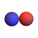
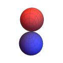
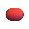
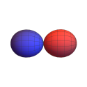
As expected, the spherical symmetry is broken: an $(l,|m|)$-dependency is introduced in the perturbed eigenvalues. In Tab.2, we provide the first order eigenvalues, which can be useful for basis set truncation purposes. We note that, at first order, degeneracy is not completely lifted, as for example, $E_{4,0,0}=E_{4,3,\pm 2}$. If we factorize by the zero order energy, we see that the relative corrections at the first order are all proportional to $\frac{\mu^{2}Z^{2}}{a}$.
A similar observation can be made for the first order corrected eigenfunctions,

$\displaystyle\psi_{n,l,m}$ $\displaystyle=$ ψn,l,m(0)+βˆ‘(nβ€²,lβ€²)β‰ (n,l)βˆ’Ο€5​(Za)β€‹βŸ¨Οˆnβ€²,lβ€²,m(0)|Y2,0​(ΞΈ,Ο•)r3|ψn,l,m(0)⟩En,l,m(0)βˆ’Enβ€²,lβ€²,m(0)β€‹Οˆnβ€²,lβ€²,m(0)subscriptsuperscriptπœ“0π‘›π‘™π‘šsubscriptsuperscript𝑛′superscriptπ‘™β€²π‘›π‘™πœ‹5π‘π‘Žquantum-operator-productsubscriptsuperscriptπœ“0superscript𝑛′superscriptπ‘™β€²π‘šsubscriptπ‘Œ20πœƒitalic-Ο•superscriptπ‘Ÿ3subscriptsuperscriptπœ“0π‘›π‘™π‘šsubscriptsuperscript𝐸0π‘›π‘™π‘šsubscriptsuperscript𝐸0superscript𝑛′superscriptπ‘™β€²π‘šsubscriptsuperscriptπœ“0superscript𝑛′superscriptπ‘™β€²π‘š\displaystyle\psi^{(0)}_{n,l,m}+\sum\limits_{(n^{\prime},l^{\prime})\neq(n,l)}\frac{-\sqrt{\frac{\pi}{5}}\left(\frac{Z}{a}\right)\langle\psi^{(0)}_{n^{\prime},l^{\prime},m}|\frac{Y_{2,0}(\theta,\phi)}{r^{3}}|\psi^{(0)}_{n,l,m}\rangle}{E^{(0)}_{n,l,m}-E^{(0)}_{n^{\prime},l^{\prime},m}}\ \psi^{(0)}_{n^{\prime},l^{\prime},m}
=\displaystyle= ψn,l,m(0)+βˆ‘(nβ€²,lβ€²)β‰ (n,l)βˆ’(Za)β€‹βˆ«0+∞Rnβ€²,l′​(r)​Rn,l​(r)r​𝑑rΓ—(βˆ’1)m​(lβ€²+12)​(l+12)​(lβ€²l2000)​(lβ€²l2βˆ’mm0)Β βˆ’ΞΌβ€‹Z22​n2+μ​Z22​n′⁣2β€‹Οˆnβ€²,lβ€²,m(0)subscriptsuperscriptπœ“0π‘›π‘™π‘šsubscriptsuperscript𝑛′superscriptπ‘™β€²π‘›π‘™π‘π‘Žsuperscriptsubscript0subscript𝑅superscript𝑛′superscriptπ‘™β€²π‘Ÿsubscriptπ‘…π‘›π‘™π‘Ÿπ‘Ÿdifferential-dπ‘Ÿ(βˆ’1)m(lβ€²+12)(l+12)(lβ€²l2000)(lβ€²l2βˆ’mm0)Β πœ‡superscript𝑍22superscript𝑛2πœ‡superscript𝑍22superscript𝑛′2subscriptsuperscriptπœ“0superscript𝑛′superscriptπ‘™β€²π‘š\displaystyle\psi^{(0)}_{n,l,m}+\sum\limits_{(n^{\prime},l^{\prime})\neq(n,l)}\frac{-\left(\frac{Z}{a}\right)\int\limits_{0}^{+\infty}\frac{R_{n^{\prime},l^{\prime}}(r)R_{n,l}(r)}{r}dr\times\mbox{\scriptsize$(-1)^{m}\sqrt{(l^{\prime}+\frac{1}{2})(l+\frac{1}{2})}\begin{pmatrix}l^{\prime}&l&2\\ 0&0&0\end{pmatrix}\begin{pmatrix}l^{\prime}&l&2\\ -m&m&0\end{pmatrix}$ }}{-\frac{\mu Z^{2}}{2n^{2}}+\frac{\mu Z^{2}}{2n^{\prime 2}}}\psi^{(0)}_{n^{\prime},l^{\prime},m}
=\displaystyle= ψn,l,m(0)+βˆ‘(nβ€²,lβ€²)β‰ (n,l)2​n′⁣2​n2a​μ​Z​(n′⁣2βˆ’n2)​(βˆ’1)m​(lβ€²+12)​(l+12)​(lβ€²l2000)​(lβ€²l2βˆ’mm0)β€‹βˆ«0+∞Rnβ€²,l′​(r)​Rn,l​(r)r​𝑑rΒ β€‹Οˆnβ€²,lβ€²,m(0),subscriptsuperscriptπœ“0π‘›π‘™π‘šsubscriptsuperscript𝑛′superscript𝑙′𝑛𝑙2n′⁣2n2aΞΌZ(n′⁣2βˆ’n2)(βˆ’1)m(lβ€²+12)(l+12)(lβ€²l2000)(lβ€²l2βˆ’mm0)∫0+∞Rnβ€²,lβ€²(r)Rn,l(r)r𝑑rΒ subscriptsuperscriptπœ“0superscript𝑛′superscriptπ‘™β€²π‘š\displaystyle\psi^{(0)}_{n,l,m}+\sum\limits_{(n^{\prime},l^{\prime})\neq(n,l)}\mbox{\scriptsize$\frac{2n^{\prime 2}n^{2}}{a\mu Z(n^{\prime 2}-n^{2})}(-1)^{m}\sqrt{(l^{\prime}+\frac{1}{2})(l+\frac{1}{2})}\begin{pmatrix}l^{\prime}&l&2\\ 0&0&0\end{pmatrix}\begin{pmatrix}l^{\prime}&l&2\\ -m&m&0\end{pmatrix}\int\limits_{0}^{+\infty}\frac{R_{n^{\prime},l^{\prime}}(r)R_{n,l}(r)}{r}dr$ }\psi^{(0)}_{n^{\prime},l^{\prime},m},

the radial integral being proportional to $\mu^{3}Z^{3}$ (because of the $\frac{1}{r^{3}}$-term, when we make the change of variables $x=2\mu Zr$), all the coupling coefficients in the expansion are proportional to $\frac{\mu^{2}Z^{2}}{a}$. Here also, the potentially divergent terms in the expansion, due to the degeneracy of the zeroth order eigenvalues for a given $n$ in the denominators, can be excluded since the corresponding numerators cancel out because of the radial integrals again.

The first terms in the expansion of the lowest eigenfunctions are given in Tab. 3.

$l=0$ $l=1$ $l=2$ $l=3$
$E_{4,1,\pm 1}=-\frac{\mu Z^{2}}{32}+\frac{\mu^{3}Z^{4}}{1920a}$
$E_{4,2,\pm 2}=-\frac{\mu Z^{2}}{32}+\frac{\mu^{3}Z^{4}}{6760a}$
$E_{4,3,\pm 3}=-\frac{\mu Z^{2}}{32}+\frac{\mu^{3}Z^{4}}{16128a}$
$n=4$ $E_{4,0,0}=-\frac{\mu Z^{2}}{32}$ $E_{4,3,\pm 2}=-\frac{\mu Z^{2}}{32}$
$E_{4,3,\pm 1}=-\frac{\mu Z^{2}}{32}-\frac{\mu^{3}Z^{4}}{26880a}$
$E_{4,3,0}=-\frac{\mu Z^{2}}{32}-\frac{\mu^{3}Z^{4}}{20160a}$
$E_{4,2,\pm 1}=-\frac{\mu Z^{2}}{32}-\frac{\mu^{3}Z^{4}}{13440a}$
$E_{4,2,0}=-\frac{\mu Z^{2}}{32}-\frac{\mu^{3}Z^{4}}{6760a}$
$E_{4,1,0}=-\frac{\mu Z^{2}}{32}-\frac{\mu^{3}Z^{4}}{960a}$
……………………………………………………………………………………………………..
$E_{3,1,\pm 1}=-\frac{\mu Z^{2}}{18}+\frac{\mu^{3}Z^{4}}{810a}$
$E_{3,2,\pm 2}=-\frac{\mu Z^{2}}{18}+\frac{\mu^{3}Z^{4}}{2835a}$
$n=3$ $E_{3,0,0}=-\frac{\mu Z^{2}}{18}$
$E_{3,2,\pm 1}=-\frac{\mu Z^{2}}{18}-\frac{\mu^{3}Z^{4}}{5670a}$
$E_{3,2,0}=-\frac{\mu Z^{2}}{18}-\frac{\mu^{3}Z^{4}}{2835a}$
$E_{3,1,0}=-\frac{\mu Z^{2}}{18}-\frac{\mu^{3}Z^{4}}{405a}$
……………………………………………………………………………………………………..
$E_{2,1,\pm 1}=-\frac{\mu Z^{2}}{8}+\frac{\mu^{3}Z^{4}}{240a}$
$n=2$ $E_{2,0,0}=-\frac{\mu Z^{2}}{8}$
$E_{2,1,0}=-\frac{\mu Z^{2}}{8}-\frac{\mu^{3}Z^{4}}{120a}$
……………………………………………………………………………………………………..
$n=1$ $E_{1,0,0}=-\frac{\mu Z^{2}}{2}$
Table 2: First-order corrected energies (up to n=4). For every pairs, $(n,l)$, the sum over $m\in\{-l,-l+1,\cdots,l-1,l\}$ of the first order corrections is zero. The spacing between the energies does not follow any scale, only the order between the levels is respected.
$n=1$ $l=0$ $m=0$ $\psi_{1,0,0}=\psi^{(0)}_{1,0,0}+\frac{\sqrt{5}}{5a\mu Z}\sum\limits_{n^{\prime}>2}\mbox{\scriptsize$\frac{1}{1-\frac{1}{n^{\prime 2}}}\int\limits_{0}^{+\infty}\frac{R_{n^{\prime},2}(r)R_{1,0}(r)}{r}dr$ }\psi^{(0)}_{n^{\prime},2,0}$
Β Β Β Β Β Β Β Β Β Β Β Β Β =ψ1,0,0(0)+ΞΌ2​Z2a​(6480β€‹Οˆ3,2,0(0)+10428125β€‹Οˆ4,2,0(0)+5​146804β€‹Οˆ5,2,0(0)+5744​2112353145β€‹Οˆ6,2,0(0)+3299​218847360β€‹Οˆ7,2,0(0)+β‹―)absentsubscriptsuperscriptπœ“0100superscriptπœ‡2superscript𝑍2π‘Ž6480subscriptsuperscriptπœ“032010428125subscriptsuperscriptπœ“04205146804subscriptsuperscriptπœ“052057442112353145subscriptsuperscriptπœ“06203299218847360subscriptsuperscriptπœ“0720β‹―=\psi^{(0)}_{1,0,0}+\frac{\mu^{2}Z^{2}}{a}\left(\frac{\sqrt{6}}{480}\psi^{(0)}_{3,2,0}+\frac{104}{28125}\psi^{(0)}_{4,2,0}+\frac{5\sqrt{14}}{6804}\psi^{(0)}_{5,2,0}+\frac{5744\sqrt{21}}{12353145}\psi^{(0)}_{6,2,0}+\frac{3299\sqrt{21}}{8847360}\psi^{(0)}_{7,2,0}+\cdots\right)
$n=2$ $l=1$ $m=0$ $\psi_{2,1,0}=\psi^{(0)}_{2,1,0}+\frac{8}{5a\mu Z}\sum\limits_{n^{\prime}>2}\mbox{\scriptsize$\frac{1}{1-\frac{4}{n^{\prime 2}}}\int\limits_{0}^{+\infty}\frac{R_{n^{\prime},1}(r)R_{2,1}(r)}{r}dr$ }\psi^{(0)}_{n^{\prime},1,0}+\frac{12\sqrt{21}}{35a\mu Z}\sum\limits_{n^{\prime}>3}\mbox{\scriptsize$\frac{1}{1-\frac{4}{n^{\prime 2}}}\int\limits_{0}^{+\infty}\frac{R_{n^{\prime},3}(r)R_{2,1}(r)}{r}dr$ }\psi^{(0)}_{n^{\prime},3,0}$
Β Β Β Β Β Β Β Β Β Β Β Β  =ψ2,1,0(0)+ΞΌ2​Z2a​(1923125β€‹Οˆ3,1,0(0)+56​106075β€‹Οˆ4,1,0(0)+8768​51058841β€‹Οˆ5,1,0(0)+201​3589600β€‹Οˆ6,1,0(0)+2926784​141076168025β€‹Οˆ7,1,0(0)+β‹―)absentsubscriptsuperscriptπœ“0210superscriptπœ‡2superscript𝑍2π‘Ž1923125subscriptsuperscriptπœ“031056106075subscriptsuperscriptπœ“0410876851058841subscriptsuperscriptπœ“05102013589600subscriptsuperscriptπœ“06102926784141076168025subscriptsuperscriptπœ“0710β‹―=\psi^{(0)}_{2,1,0}+\frac{\mu^{2}Z^{2}}{a}\left(\frac{192}{3125}\psi^{(0)}_{3,1,0}+\frac{56\sqrt{10}}{6075}\psi^{(0)}_{4,1,0}+\frac{8768\sqrt{5}}{1058841}\psi^{(0)}_{5,1,0}+\frac{201\sqrt{35}}{89600}\psi^{(0)}_{6,1,0}+\frac{2926784\sqrt{14}}{1076168025}\psi^{(0)}_{7,1,0}+\cdots\right)
Β Β Β Β Β Β Β Β Β Β Β Β Β Β Β Β Β Β Β Β Β Β Β Β Β Β  +ΞΌ2​Z2a​(8​1014175β€‹Οˆ4,3,0(0)+512​5823543β€‹Οˆ5,3,0(0)+123​10358400β€‹Οˆ6,3,0(0)+541184​31076168025β€‹Οˆ7,3,0(0)+β‹―)superscriptπœ‡2superscript𝑍2π‘Ž81014175subscriptsuperscriptπœ“04305125823543subscriptsuperscriptπœ“053012310358400subscriptsuperscriptπœ“063054118431076168025subscriptsuperscriptπœ“0730β‹―+\frac{\mu^{2}Z^{2}}{a}\left(\frac{8\sqrt{10}}{14175}\psi^{(0)}_{4,3,0}+\frac{512\sqrt{5}}{823543}\psi^{(0)}_{5,3,0}+\frac{123\sqrt{10}}{358400}\psi^{(0)}_{6,3,0}+\frac{541184\sqrt{3}}{1076168025}\psi^{(0)}_{7,3,0}+\cdots\right)
$n=2$ $l=0$ $m=0$ $\psi_{2,0,0}=\psi^{(0)}_{2,0,0}+\frac{4\sqrt{5}}{5a\mu Z}\sum\limits_{n^{\prime}>2}\mbox{\scriptsize$\frac{1}{1-\frac{4}{n^{\prime 2}}}\int\limits_{0}^{+\infty}\frac{R_{n^{\prime},2}(r)R_{2,0}(r)}{r}dr$ }\psi^{(0)}_{n^{\prime},2,0}$
Β Β Β Β Β Β Β Β Β Β Β Β Β =ψ2,0,0(0)βˆ’ΞΌ2​Z2a​(32​39375β€‹Οˆ3,2,0(0)+2​21215β€‹Οˆ4,2,0(0)+3680​77411887β€‹Οˆ5,2,0(0)+29​42215040β€‹Οˆ6,2,0(0)+63584​42645700815β€‹Οˆ7,2,0(0)+β‹―)absentsubscriptsuperscriptπœ“0200superscriptπœ‡2superscript𝑍2π‘Ž3239375subscriptsuperscriptπœ“0320221215subscriptsuperscriptπœ“0420368077411887subscriptsuperscriptπœ“05202942215040subscriptsuperscriptπœ“06206358442645700815subscriptsuperscriptπœ“0720β‹―=\psi^{(0)}_{2,0,0}-\frac{\mu^{2}Z^{2}}{a}\left(\frac{32\sqrt{3}}{9375}\psi^{(0)}_{3,2,0}+\frac{2\sqrt{2}}{1215}\psi^{(0)}_{4,2,0}+\frac{3680\sqrt{7}}{7411887}\psi^{(0)}_{5,2,0}+\frac{29\sqrt{42}}{215040}\psi^{(0)}_{6,2,0}+\frac{63584\sqrt{42}}{645700815}\psi^{(0)}_{7,2,0}+\cdots\right)
$n=2$ $l=1$ $m=\pm 1$ $\psi_{2,1,\pm 1}=\psi^{(0)}_{2,1,\pm 1}-\frac{4}{5a\mu Z}\sum\limits_{n^{\prime}>2}\mbox{\scriptsize$\frac{1}{1-\frac{4}{n^{\prime 2}}}\int\limits_{0}^{+\infty}\frac{R_{n^{\prime},1}(r)R_{2,1}(r)}{r}dr$ }\psi^{(0)}_{n^{\prime},1,\pm 1}$
Β Β Β Β Β Β Β Β Β Β Β Β Β Β Β Β Β Β Β Β Β Β Β Β Β Β Β Β Β Β  +12​1435​a​μ​Zβ€‹βˆ‘nβ€²>311βˆ’4n′⁣2β€‹βˆ«0+∞Rnβ€²,3​(r)​R2,1​(r)r​𝑑rΒ β€‹Οˆnβ€²,3,Β±1(0)121435π‘Žπœ‡π‘subscriptsuperscript𝑛′311βˆ’4n′⁣2∫0+∞Rnβ€²,3(r)R2,1(r)r𝑑rΒ subscriptsuperscriptπœ“0superscript𝑛′3plus-or-minus1+\frac{12\sqrt{14}}{35a\mu Z}\sum\limits_{n^{\prime}>3}\mbox{\scriptsize$\frac{1}{1-\frac{4}{n^{\prime 2}}}\int\limits_{0}^{+\infty}\frac{R_{n^{\prime},3}(r)R_{2,1}(r)}{r}dr$ }\psi^{(0)}_{n^{\prime},3,\pm 1}
$=\psi^{(0)}_{2,1,\pm 1}-\frac{\mu^{2}Z^{2}}{a}\left(\frac{96}{3125}\psi^{(0)}_{3,1,\pm 1}+\frac{28\sqrt{10}}{18225}\psi^{(0)}_{4,1,\pm 1}+\frac{4384\sqrt{5}}{1058841}\psi^{(0)}_{5,1,\pm 1}+\frac{201\sqrt{35}}{179200}\psi^{(0)}_{6,1,\pm 1}+\frac{1463392\sqrt{14}}{1076168025}\psi^{(0)}_{7,1,\pm 1}+\cdots\right)$
$\qquad\qquad+\frac{\mu^{2}Z^{2}}{a}\left(\frac{16\sqrt{15}}{42525}\psi^{(0)}_{4,3,\pm 1}+\frac{512\sqrt{30}}{2470629}\psi^{(0)}_{5,3,\pm 1}+\frac{41\sqrt{15}}{179200}\psi^{(0)}_{6,3,\pm 1}+\frac{541184\sqrt{2}}{1076168025}\psi^{(0)}_{7,3,\pm 1}+\cdots\right)$
n=3𝑛3n=3 l=1𝑙1l=1 m=0π‘š0m=0 ψ3,1,0=ψ3,1,0(0)+185​a​μ​Zβ€‹βˆ‘nβ€²>1nβ€²β‰ 311βˆ’9n′⁣2β€‹βˆ«0+∞Rnβ€²,1​(r)​R3,1​(r)r​𝑑rΒ β€‹Οˆnβ€²,1,0(0)+27​2135​a​μ​Zβ€‹βˆ‘nβ€²>311βˆ’9n′⁣2β€‹βˆ«0+∞Rnβ€²,3​(r)​R3,1​(r)r​𝑑rΒ β€‹Οˆnβ€²,3,0(0)subscriptπœ“310subscriptsuperscriptπœ“0310185π‘Žπœ‡π‘subscriptsuperscript𝑛′1superscript𝑛′311βˆ’9n′⁣2∫0+∞Rnβ€²,1(r)R3,1(r)r𝑑rΒ subscriptsuperscriptπœ“0superscript𝑛′10272135π‘Žπœ‡π‘subscriptsuperscript𝑛′311βˆ’9n′⁣2∫0+∞Rnβ€²,3(r)R3,1(r)r𝑑rΒ subscriptsuperscriptπœ“0superscript𝑛′30\psi_{3,1,0}=\psi^{(0)}_{3,1,0}+\frac{18}{5a\mu Z}\sum\limits_{\begin{subarray}{c}n^{\prime}>1\\ n^{\prime}\neq 3\end{subarray}}\mbox{\scriptsize$\frac{1}{1-\frac{9}{n^{\prime 2}}}\int\limits_{0}^{+\infty}\frac{R_{n^{\prime},1}(r)R_{3,1}(r)}{r}dr$ }\psi^{(0)}_{n^{\prime},1,0}+\frac{27\sqrt{21}}{35a\mu Z}\sum\limits_{n^{\prime}>3}\mbox{\scriptsize$\frac{1}{1-\frac{9}{n^{\prime 2}}}\int\limits_{0}^{+\infty}\frac{R_{n^{\prime},3}(r)R_{3,1}(r)}{r}dr$ }\psi^{(0)}_{n^{\prime},3,0}
$=\psi^{(0)}_{3,1,0}+\frac{\mu^{2}Z^{2}}{a}\left(\frac{-192}{3125}\psi^{(0)}_{2,1,0}+\frac{60288\sqrt{10}}{2941225}\psi^{(0)}_{4,1,0}+\frac{231\sqrt{5}}{16384}\psi^{(0)}_{5,1,0}+\frac{35648\sqrt{35}}{10333575}\psi^{(0)}_{6,1,0}+\frac{310191\sqrt{14}}{78125000}\psi^{(0)}_{7,1,0}+\cdots\right)$
Β Β Β Β Β Β Β Β Β Β Β Β Β Β Β Β Β Β Β Β Β Β Β Β Β Β  βˆ’ΞΌ2​Z2a​(10368​1020588575β€‹Οˆ4,3,0(0)+81​5458752β€‹Οˆ5,3,0(0)+128​103444525β€‹Οˆ6,3,0(0)+567​339062500β€‹Οˆ7,3,0(0)+β‹―)superscriptπœ‡2superscript𝑍2π‘Ž103681020588575subscriptsuperscriptπœ“0430815458752subscriptsuperscriptπœ“0530128103444525subscriptsuperscriptπœ“0630567339062500subscriptsuperscriptπœ“0730β‹―-\frac{\mu^{2}Z^{2}}{a}\left(\frac{10368\sqrt{10}}{20588575}\psi^{(0)}_{4,3,0}+\frac{81\sqrt{5}}{458752}\psi^{(0)}_{5,3,0}+\frac{128\sqrt{10}}{3444525}\psi^{(0)}_{6,3,0}+\frac{567\sqrt{3}}{39062500}\psi^{(0)}_{7,3,0}+\cdots\right)
Table 3: First-order corrected wave functions, ordered in increasing energy eigenvalue up to n=4 (in Appendix we provide a more comprehensive table up to n=7, β€œi-orbitals”).
$1s$ $2p_{z}$ $2p_{x}$
$V(\vec{r})=\frac{-Z}{||\vec{r}||}$ Refer to caption Refer to caption Refer to caption
$V(\vec{r})=-Z\sqrt{\frac{a}{\pi}}\int\limits_{-\infty}^{+\infty}\frac{exp[-az_{0}^{2}]}{||\vec{r}-\vec{r_{z_{0}}}||}dz_{0}$ Refer to caption Refer to caption Refer to caption
Figure 1: Comparison of hydrogenoid and smeared Coulomb potential orbitals. The orbitals represented in the second row correspond are the first order correction for a first order expansion of the smeared Coulomb potential in $\frac{1}{a}$ as $a\rightarrow+\infty$. The parameters are tuned so that the corrective contributions are about $10\%$ of the unperturbed solutions displayed in the first row.

3 Conclusion

In this study, we have obtained first order perturbative corrections to the eigenfunctions of a smeared Coulomb potential along an arbitrary axis. Such a potential can represent the potential felt by an electron bounded to a vibrating nucleus of effective charge $Z$, effective reduced mass $\mu$ and effective classical vibrating amplitude equal to $\sqrt{\frac{2n_{vib}+1}{2a}}$ (in harmonic quantum level $n_{vib}$). Hence, it is hoped that these approximate eigenstates can be appropriate to describe the electron density of the effective electronic Hamiltonians solved in the EN-MFCI method. On the practical side, it can be taken advantage of the remarkable fact that, only a single parameter, namely $\frac{\mu^{2}Z^{2}}{a}$, need to be optimized for all the basis functions.

Furthermore, the DHO basis functions can be seen as contracted STO, corresponding to different angular momenta. So, the codes and techniques already developed for STO basis functions, can conveniently be employed to compute the multicenter integrals, that are needed for molecular computations with these new basis functions.

A hyperbolic cosine factor can be associated to ETO to provide a β€œdouble zeta” character to a minimal basis set 14. This can be considered for DHO, as well. However, one can also combine different sets of DHO corresponding to atoms at different ionization states, for example, to obtain proper multi-zeta basis sets.

Beside the application to the EN-MFCI method, these orbitals could be useful for β€œclamped nuclei” quantum chemistry calculations, as they can be regarded as naturally β€œhybridized” (unlike spherical harmonics STO). One can develop a battery of model Hamiltonian adapted to one or several bond directions (whatever a chemical bond might be from the quantum mechanical point of view) and obtain their first order approximate eigenfunctions by following the approach presented in this paper. For example, different shapes of Coulomb potentials could provide different model Hamitonians for the sp, sp2, or sp3 hybridization of a carbon atom, and in turn, relevant naturally-hybridized orbital eigenfunction basis sets.

Another potential application for β€œclamped nuclei” quantum chemistry is to save on polarization orbital sets, since high angular momentum atomic primitives are already contracted within our orbitals.

References

  • 1 P. Cassam-ChenaΓ―, D. Jayatilaka, G.S. Chandler, LABEL:Journal_de_Chimie_Physique9522411998
  • 2 S. F. Boys and F. Bernardi, LABEL:Mol._Phys.195531970
  • 3 I.I. Guseinov, E. Sahin and M. Erturk, LABEL:Mol._Phys.112352014
  • 4 C. Zener, LABEL:Phys._Rev.36511930
  • 5 J.C. Slater, LABEL:Phys._Rev.36571930
  • 6 E. Filter and E. O. Steinborn, LABEL:Phys._Rev.A1811978
  • 7 H. Shull, P.-O. LΓΆwdin, J.Β Chem.Β Phys.306171959
  • 8 James Emil Avery, LABEL:Advances_in_Quantum_Chemistry67129-1512013
  • 9 James Emil Avery and John Scales Avery, LABEL:Advances_in_Quantum_Chemistry70265-3242015
  • 10 James Emil Avery and John Scales Avery, LABEL:Advances_in_Quantum_Chemistry76133-1462018
  • 11 P. Cassam-ChenaΓ―, B. Suo, W. Liu, LABEL:Phys._Rev.A920125022015
  • 12 P. Cassam-ChenaΓ―, B. Suo, W. Liu, LABEL:Theor._Chim._Acta.136522017
  • 13 H. Taşeli, $\dot{\text{I}}$nci M. Erhan and Γ–. UΗ§ur, LABEL:J._Math._Chem.323232002
  • 14 E. Sahin, T. Ozdogan, M. Orbay, LABEL:J._Math._Chem.5518492017