The Mg i b triplet and the 4571 Å line as diagnostics of stellar chromospheric activity

Abstract

Context. The Mg i 4571 Å line and the $b$ triplet are denoted in the literature as diagnostics of solar and stellar activity since their formation is in the low chromosphere.

Aims. To investigate the potential of these four spectral lines as diagnostics of chromospheric activity in solar-like stars, studying the dependence of the intensity of these lines from local atmospheric changes by varying atmospheric models and stellar parameters.

Methods. Starting with Next-Gen photospheric models, we build a grid of atmospheric models including photosphere, chromosphere and transition region and solve the radiative transfer to obtain synthetic profiles to compare with observed spectra of main-sequence, solar like stars with effective temperatures in the range $4800-6400$ K, solar gravity and solar metallicity.

Results. We find that the Mg i 4571 Å line is significantly sensitive to local changes in the atmospheric model around the minimum temperature. Instead, the lines of the $b$ triplet do not show significant responses to changes on the local atmospheric structure.

1 Introduction

Stellar chromospheres are classically defined as an atmospheric layer lying above the photosphere and below the corona, characterized by a positive temperature gradient and a marked departure from radiative equilibrium. Stellar chromospheres exhibit a wide range of phenomena collectively called “activity”, mainly due to the presence and time evolution of highly structured magnetic fields emerging from the convective envelope. Strong spectral lines are commonly used as diagnostics of chromospheric activity, such as Ca ii H and K lines and the infrared triplet, the H$\alpha$ line whose core is formed in the chromosphere, the Na i D lines, and many UV lines from atoms and ions such as O i, C i, and Fe ii, with formation temperature at $\sim$10⁴ K.

Historically, magnetic activity in stellar atmospheres has been confirmed from long-term observations of the spectroscopic and photometric behavior of Sun-like stars in the Ca ii H and K lines. In particular, most of the data have been collected in two projects, one at Mount Wilson Observatory (MWO; Wilson 1978; Duncan et al. 1991) and another at Lowell Observatory (Hall et al. 2007). The observed line emissions, resulting from the non-thermal heating that occurs in the presence of strong magnetic fields, are quantified through the $S$ (Wilson 1978) and $R^{\prime}_{HK}$ (Noyes et al. 1984) indices.

In this work, we investigate the potential of four Mg i spectral lines, the 4571 Å line and the $b$ triplet at 5183, 5172 and 5167 Å, as diagnostics of chromospheric activity in solar-like stars. These lines have been modeled and observed in the solar atmosphere by many authors (i.e., Athay & House 1962; Athay & Canfield 1969; Altrock & Cannon 1972; White et al. 1972; Altrock & Canfield 1974; Heasley & Allen 1980) and are known as spectroscopic probes of physical conditions in the solar upper photosphere and lower chromosphere. For these reasons they are well suited as a diagnostic of the low chromosphere, close to the temperature minimum region. Langangen et al. (2009) studied the Mg i 4571 Å theoretical line formation in the quiet Sun and in a series of sunspot models, concluding that the line can be used to probe the lower chromosphere, especially for cooler atmospheres, such as sunspots.

The Mg i 4571 Å line is a ”forbidden”, intersystem line originating between the atomic levels $3^{1}S$ and $3^{3}P_{1}$ and, in the Sun, forms at about 500 km above $\tau_{5000}=1$ (see also discussion in Sec. 2.1 and in particular the lower panel of Fig. 2). Its source function is very close to local thermodynamical equilibrium (LTE) because the population ratio of its upper and lower levels is determined mainly by collisional processes. Despite its small oscillator strength ($2.4\times 10^{-6}$) it is a prominent line in the solar spectrum because its opacity is determined by the population of the Mg i ground state. This also implies that non local thermodynamical equilibrium (NLTE) effects may be important in determining its optical depth. Hence the need of full, NLTE, multi-level calculations.

The Mg i $b$ triplet originates between the atomic levels $3^{3}P_{0,1,2}$ and $4^{3}D$, and comprises a component at 5183 Å with $J_{l}=2$ ($b_{1}$), one at 5172 Å with $J_{l}=1$ ($b_{2}$) and one at 5167 Å with $J_{l}=0$ ($b_{3}$). The relative simplicity of the formation of the Mg i 4571 line is in contrast with the complex formation of the Mg i $b$ triplet. In the solar atmosphere the cores of the $b$ triplet lines form in the low chromosphere. Both their source function and opacities are affected by NLTE, mainly though photoionization. The coupling with other atmospheric regions introduced by this kind of NLTE effects makes these lines less sensitive to local conditions. The wings of these lines form in the photosphere (Zhao et al. 1998; Sasso 2004).

The behavior and the formation of these Mg lines have been studied also in stellar atmospheres and, in particular, the Mg i $b$ triplet has been often indicated in the literature as a good diagnostic of stellar activity (Montes et al. 1999a, b; Basri et al. 1989). Recently, Osorio et al. (2015) and Osorio & Barklem (2016) studied the Mg line formation in late-type stellar atmospheres, using the same numerical code to solve the coupled equations of radiative transfer and statistical equilibrium we are using in this work and describe in Sec. 2. They constructed a new Mg model atom for NLTE studies and implemented new quantum mechanical calculations to investigate the effect of different collisional processes in benchmark late-type stars. Their study aims to give abundance corrections especially in metal-poor stars, where departures from LTE affect line formations. A similar attempt has been done by Merle et al. (2011) for the Mg line formation in late-type giant and supergiant stars, and in particular for the lines we are studying, also in a metal-poor dwarf and a metal-poor giant (Merle et al. 2013a, b).

In this work, we extend the above investigation to solar-like stars (dwarf stars of spectral types F-K and solar metallicity) by studying the dependence of the intensity of these lines from local atmospheric changes by varying atmospheric models and stellar parameters. The aim is to evaluate the reliability of these four Mg spectral lines as diagnostics of chromospheric activity in this type of stars.

The paper is structured as follows. In Sec. 2 we describe the Mg atomic model and the stellar atmospheric models we used in this work. In Sec. 3, we compare the synthetic profiles obtained with eight observed spectra of Sun-like stars and discuss the sensitivity of the Mg lines to local changes in the atmospheric model. Finally, in the conclusions (Sec. 4), the role of these Mg lines as diagnostic of chromospheric activity is defined.

2 Model calculations and solar test

In order to investigate the sensitivity of the Mg i 4571 Å and the $b$ triplet line profiles in main-sequence, solar-like stars to local atmospheric changes at chromospheric levels, we built a grid of models of a stellar atmosphere with different effective temperatures, solar gravity and solar metallicity and solved the coupled equations of radiative transfer and statistical equilibrium were solved for the Mg i using version 2.2 of the code MULTI (Carlsson 1986).

2.1 Atomic model

In this work we used, with some modifications, the Mg i atomic model proposed by Carlsson et al. (1992), consisting of 66 levels (including the continuum), 315 lines and 65 bound-free ($b-f$) transitions treated in detail. The atomic model was slightly modified by Carlsson (private communication) with respect to the original one presented in the above publication. The modifications were done in order to analyze in detail the Mg $b$ triplet that it is treated as a superposition of three lines, taking into account that they are close enough to affect each other. The photo-ionization cross-sections are given with many more wavelength points which makes the line blanketing calculation more accurate. In the literature we found other Mg atomic models containing different numbers of atomic levels. Mauas et al. (1988) used a 12-level atomic model to study the influence that the uncertainties in the value of different atomic parameters may have on the calculated profiles, comparing them with the Sun spectrum. Zhao et al. (1998) and Zhao & Gehren (2000) presented an 84-level atomic model to investigate the formation of neutral Mg lines in the solar photosphere and in the photosphere of cool stars, respectively. Their model is nearly the same as that used by Carlsson et al. (1992). Mashonkina et al. (1996) and Shimanskaya et al. (2000) instead, used a 49-level Mg i atomic model to study the formation of Mg lines in the atmospheres of stars of various spectral types performing a detailed statistical-equilibrium analysis. Finally, there are two recent atomic models constructed by Merle et al. (2011) and Osorio et al. (2015), used to investigate the effect of NLTE Mg line formation in late-type stellar atmospheres, as described in Sec. 1. Results from these papers show that departures from LTE for the lines we are considering are significant for low metallicity stars. We decided to use the model proposed by Carlsson et al. (1992) because its original use is closer to our study and treats specifically the Mg $b$ triplet. Moreover, we want to compare the results of the line synthesis with observed spectra from solar-like stars (stars with solar metallicity). All the atomic parameters used are specified in the work of Carlsson et al. (1992).

In order to match the observed profiles and test the procedure on the Sun, we recalculated the Van der Waals damping parameter for the transitions involved in the formation of the lines of our interest. As pointed out by Mauas et al. (1988), the Van der Waals broadening dominates over the radiative and the Stark broadenings in determining the Voigt coefficient in the formation of the 5173 Å line (studied as representative of the whole triplet). We recalculated also the Van der Waals damping parameter for the 4571 Å line, for homogeneity. The value of the theoretical Van der Waals damping parameter, $\Gamma_{\rm VW}$, has been calculated with two different methods, following the theoretical models presented by Deridder & van Rensbergen (1976) and by Anstee & O’Mara (1995). The values retrieved are respectively 2.55 and 4.43 ($10^{-8}$ rad cm${}^{3}/$s) for the $b$ triplet and 0.86 and 1.25 ($10^{-8}$ rad cm${}^{3}/$s) for the 4571 Å line. The Van der Waals damping coefficient required in the atomic model is the factor $f_{\rm GVW}$ in the following formula

$$\Gamma_{\rm VW}=f_{\rm GVW}\;\Gamma_{\rm VWM},$$ (1)

where $\Gamma_{\rm VWM}$ is the value of the broadening calculated by the program MULTI, as follows (Milahas 1978, Sec. 9.3)

$$\Gamma_{\rm VWM}=8.08\left(1+0.41\left(\frac{N_{He}}{N_{H}}\right)\right)V_{H}^{0.6}\;N_{H}\;C_{6}^{0.4},$$ (2)

where

$$V_{H}^{0.6}=\left[\frac{8kT}{\pi}\left(\frac{1}{m_{H}}+\frac{1}{m_{Mg}}\right)\right]^{0.3}$$ (3)

and

$$C_{6}=1.01\;10^{-32}(13.6\;I)^{2}\left[\frac{1}{(E_{c}-E_{u})^{2}}-\frac{1}{(E_{c}-E_{l})^{2}}\right].$$ (4)

The quantities $N_{He}$ and $N_{H}$ are, respectively, the helium and hydrogen atomic number density ($N_{He}/N_{H}=0.1$), $k$ is the Boltzmann constant, $T$ is the temperature in K, $m_{H}$ and $m_{Mg}$ are, respectively, the atomic weight of hydrogen and magnesium in g, $I$ is the ionization state of the lower transition level, $E_{c}$, $E_{u}$ and $E_{l}$ are the continuum, upper and lower level energy.

We adopt the values of the Van der Waals damping ($f_{\rm GVW}=\Gamma_{\rm VW}/\Gamma_{\rm VWM}$) that give the better agreement with the solar observed profiles: $f_{\rm GVW}=2.3$ for the $b$ triplet (the same value used by Carlsson et al. 1992) and $f_{\rm GVW}=1.1$ for the 4571 Å line (in the original atomic model was 10.9).

As it is pointed out in Langangen et al. (2009) and Carlsson et al. (1992), it is important to treat the line blanketing in order to get the ionization balance right. For this reason, some treatment of line-opacity needs to be included in the calculations. The opacity package that comes with the code takes into account free-free opacity, Rayleigh scattering, and bound-free transitions from hydrogen and metals. The absence of line blanketing in the standard opacity package leads to an overestimate of emerging intensities (especially in the UV) and therefore to an overestimate of photoionization rates, some of which can be important in NLTE calculations. We have estimated the effect of line blanketing by increasing the background standard opacity by a suitable factor, following the method described in Busà et al. (2001). This method is based on a semi-empirical approach: any background opacity source missing from the calculations is estimated from the ratio of the calculated flux to the observed one (in this work, we take the Next-Gen fluxes Allard & Hauschildt 1995, as our ”observed” reference spectrum). This approach therefore provides a quick, albeit approximate way to take into account line haze, either in LTE or NLTE, in the most relevant photoionization rates. In particular, there is no guarantee that the depth dependence of the photoionization rates is correctly computed throughout the atmosphere. But this method already provides some improvements on the modeling of the Mg i lines as we show below.

We tested our procedure and data set on the Sun using three different quiet-Sun atmospheric models. The three semi-empirical models of the solar atmosphere used, are the ones proposed by Vernazza et al. (VALC, 1981), Fontenla et al. (FALC, 1993), and Avrett & Loeser (ALC, 2008), encompassing both the photosphere and the chromosphere. Figure 1 shows the synthetic Mg i 4571 Å (left panel) and $b_{2}$ (middle and right panel) line profiles obtained using the Mg i atomic model and the three atmospheric models (VALC red dotted, FALC green dashed, and ALC blue dash-dotted line), compared with the Kitt Peak solar flux atlas (black solid line, Kurucz et al. 1984). The synthetic profiles are broadened for the value of the projected rotational velocity, $v\sin i=1.7$ km/s (Liu et al. 2015). The differences in the atmospheric models give a first indication of the sensitivity of the studied lines to changes in the atmosphere. The VALC model has the lowest minimum temperature value and the steepest temperature gradient towards the minimum. Therefore, the 4571 Å line, forming in LTE around the minimum temperature region, shows a deeper core. Indeed, the main correction made to the VALC model that brought to the construction of new models, like the FALC and the ALC, was the inclusion of more line haze lines so that the temperature gradient towards the minimum became less steep from less overionization. The $b$ triplet does not seem to be affected by any change in the atmospheric model. The best agreement with the observed spectrum is obtained with the FALC model that has a higher minimum temperature value and a less steep temperature gradient towards the minimum with respect to the VALC model.

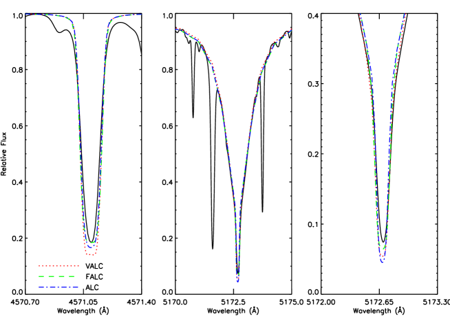
Figure 1: Mg i 4571 Å (left panel) and 5173 Å ($b_{2}$, middle and right panel) observed and synthetic line profiles for the Sun. The third panel magnifies the $b_{2}$ core. The black solid lines are the observed profiles (Kitt Peak solar flux atlas, Kurucz et al. 1984) while the red dotted, green dashed and blue dash-dotted lines are the synthetic profiles obtained by using three different atmospheric models, VALC, FALC and ALC, respectively.

We also made some tests to show how the method to treat the background line-opacity, described in Busà et al. (2001), improves the modeling of the Mg i lines. In Fig. 2 (upper panel) we plot, as an example, the synthetic profiles of the $b_{2}$ line obtained with the ALC model of the solar atmosphere with (dashed line) and without (dotted line) line blanketing. The solid line is the observed profile. For the 4571 Å line, in the lower panel of Fig. 2, we plot the contribution function to line depression (Magain 1986) versus height, for the same atmospheric model as in the upper panel with (dashed line) and without (dotted line) line blanketing. When we do not take into account any correction to the MULTI background opacity, the line forms at lower heights in the solar atmosphere, and therefore becomes less sensitive to changes in the chromosphere and at the temperature minimum (see discussion in Sec. 3).

Figure 2: Upper panel: synthetic profiles of the Mg i $b_{2}$ line obtained with the ALC model of the solar atmosphere with (dashed line) and without (dotted line) line blanketing. The solid line is the observed profile. Lower panel: contribution function to line-depression (erg cm³ s^-1 Å^-1) for the 4571 Å line versus height, for the same atmospheric model as in the upper panel, with (dashed line) and without (dotted line) line blanketing.

2.2 Atmospheric models

We selected from the Next-Gen database a grid of photospheric models of a stellar atmosphere with effective temperatures $T_{\rm{eff}}=4800,5200,5600,5800,6200$ and $6400$ K, solar gravity and solar metallicity, i.e. $\log g=4.5$ and $\left[\textmd{A}/\textmd{H}\right]=0.0$. Starting from the photospheric models, we built a grid of atmospheres including photosphere, chromosphere and transition region (TR). The chromosphere is represented by a linear dependence of the temperature as a function of $\log m$. We indicate with $\log m_{0}$ (column mass value) the point where it starts in the photosphere and with the coordinates ($\log m_{1}$, $T_{1}$) the point where the chromosphere ends and the TR starts. By giving the value of $\log m_{0}$, we fix the minimum value of the temperature in the atmospheric model, and, by giving ($\log m_{1}$, $T_{1}$) we fix the thickness of the chromosphere and the temperature gradient. We also need to specify the temperature gradient in the TR by giving the value of the last point of the model ($\log m_{2}$, $T_{2}$). We used, as for the chromospheric segment, a linear dependence of $T$ as a function of $\log m$ and for all the models the transition region gradient is the same. The values of $\log m_{0}$, $\log m_{1}$, $T_{1}$, $\log m_{2}$ and $T_{2}$ are indicated in Tab. 1 for the six models created from the same starting photosphere for each photospheric model, identified by the effective temperature, $T_{\rm{eff}}$. We refer to the different models with the names indicated in the first column, given by the values of $\log m_{0}$, $\log m_{1}$, and $T_{1}$. The names of the models are defined as mxx_myy_zzz where xx$=-\log m_{0}\times 10$, yy$=-\log m_{1}\times 10$ and zzz$=T_{1}/100$. The most active models are the ones with a higher value of $\log m_{0}$ (the chromosphere starts deeper in the photosphere) and/or a steeper chromospheric temperature gradient. Fig. 3 shows as an example six atmospheric models created by starting from a photosphere with $T_{\rm{eff}}=6200$ K, $\log g=4.5$ and $\left[\textmd{A}/\textmd{H}\right]=0.0$. We did not consider the possibility of $\log m_{1}$ greater than $-6$. Considering the formation depth in the solar atmosphere of the lines studied in this paper, their profiles should not be influenced by a change in the atmospheric model occurring in the upper chromosphere.

Figure 3: Atmospheric models obtained by adding a chromosphere and a transition region to the Next-Gen photosphere with $T_{\rm{eff}}=6200$ K. The six models differ in the chromospheric temperature gradient and/or the temperature minimum value as indicated in Table 1.

Table 1: Values of $\log m$ (g/cm²) and $T$ (K) used to build the six atmospheric models starting from the Next-Gen photospheres. $\log m_{0}$ is the starting point of the chromospheric segment in the photosphere (minimum temperature of the model). ($\log m_{1}$, $T_{1}$) are the coordinates of the end point of the chromospheric segment; the transition region ends at the point ($\log m_{2}$, $T_{2}$).

Model	$\log m_{0}$	$\log m_{1}$	$\log m_{2}$	$T_{1}$	$T_{2}$
m10_m60_075	-1.0	-6.0	-6.1	7500	100000
m10_m60_100	-1.0	-6.0	-6.1	10000	100000
m15_m60_075	-1.5	-6.0	-6.1	7500	100000
m15_m60_100	-1.5	-6.0	-6.1	10000	100000
m20_m60_075	-2.0	-6.0	-6.1	7500	100000
m20_m60_100	-2.0	-6.0	-6.1	10000	100000

3 Results

3.1 Stellar spectra

In order to compare the obtained synthetic profiles with observed ones, we selected eight stellar spectra from the high resolution (R=80000) and high SNR (300-500) UVES Paranal Observatory Project (UVES POP) library (Bagnulo et al. 2003). The chosen stars have solar gravity and solar metallicity and effective temperatures in the range $\sim 4800-6400$ K, show magnetic activity and all the Mg lines under study are available in the UVES POP library. Table 2 presents the atmospheric parameters of the selected stars collected from the literature. The first column shows the ID of the star, the second column gives the effective temperature, the third column provides the iron abundance and the fourth the surface gravity. The fifth column gives the projected rotational velocity and the last column gives the level of activity measured with two different activity index $R^{\prime}_{HK}$ or $R^{\prime}_{8662}$, depending on the star and the measurement available in the literature. Traditionally the Ca ii H and K resonance lines at 3968 and 3934 Å have been used as chromospheric diagnostics. However, observations of these lines in faint stars can be difficult, due to often low stellar flux in the blue, and the relatively poor blue response of many CCD detectors. In contrast, the Ca ii infrared triplet lines at 8498, 8542, and 8662 Å are strong and their location in the red makes them more suitable for CCD observations (Soderblom et al. 1993; Andretta et al. 2005; Busà et al. 2007; Marsden et al. 2009). The values of gravity and metallicity are not available for all the stars in the literature. (We recall that the atmospheric models are built starting from photospheres of solar gravity and metallicity, $\log g=4.5$ and $\left[\textmd{A}/\textmd{H}\right]=0.0$).

Table 2: Temperature, gravity, iron abundance, projected rotational velocity and activity index. References: ¹Soubiran et al. (2008),²Mermilliod et al. (2009), ³Gomez da Silva et al. (2014), ⁴Marsden et al. (2009), ⁵D’Orazi & Randich (2009), ⁶Battistini & Bensby (2015), ⁷Nördstrom et al. (2004), ⁸Henry et al. (1996), ⁹Casagrande et al. (2011), ¹⁰Stauffer et al. (1989), ¹¹Marsden et al. (2014), ¹²Katsova & Livshits (2011), ¹³Cenarro et al. (2007), ¹⁴Glebocki & Gnaciǹski (2005).

ID	$T_{\rm{eff}}$ (K)	$\log g$	$\left[\textmd{Fe}/\textmd{H}\right]$	$v\sin i$ (km/s)	$\log\left(R^{\prime}_{HK}\right)$	$\log\left(R^{\prime}_{8662}\right)$
HD 73722	$6480^{1}$	$4.30^{1}$	$-0.05^{1}$	$8.7\pm 0.8^{2}$	$-4.92^{3}$
IC 2391 73	$6080^{4}$	$4.45^{5}$	$0.00^{5}$	$8.4\pm 0.7^{2}$		$-4.49^{4}$
HD 211415	$5825^{6}$	$4.40^{6}$	$-0.23^{6}$	$3^{7}$	$-4.86^{8}$
HD 74497	$5642^{9}$		$-0.12^{9}$	$7^{7}$	$-4.81^{8}$
IC 2391 98	$5201^{10}$			$12.6^{2}$		$-4.89^{4}$
HD 149661	$5216^{6}$	$4.60^{6}$	$-0.01^{6}$	$2.2\pm 0.4^{11}$	$-4.57^{12}$
HD 22049	$5135^{1}$	$4.70^{1}$	$-0.07^{1}$	$8^{13}$	$-4.52^{12}$
HD 209100	$4754^{1}$	$4.45^{1}$	$-0.20^{1}$	$2.0^{14}$	$-4.57^{8}$

Figure 4 shows the observed profiles of the stars in Tab. 2 for the spectral lines we are studying, the 4571 Å line (left panel) and the central line of the $b$ triplet at 5173 Å (middle and right panel). The profiles differ mainly because of the different effective temperatures of the stars. Both lines show a less deep core and a larger width with increasing temperature. The only star that displays a different behavior, showing a less deep core than expected is the IC 2391 98. This happens because the core depth and the width of the lines are influenced also by the value of $v\sin i$ (less deep core and larger width with increasing projected rotational velocity) and this star has the largest value of $v\sin i$ with respect to all the other stars.

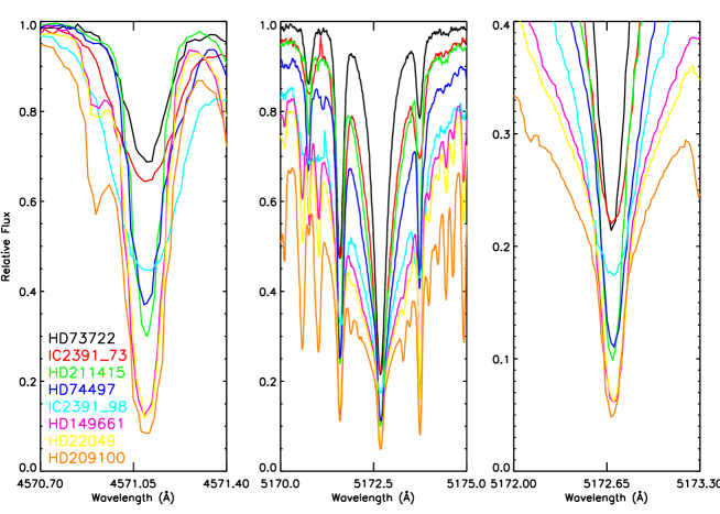
Figure 4: Mg i 4571 Å (left panel), $b_{2}$ at 5173 Å (middle) and $b_{2}$ core (right) observed line profiles for the stars in Tab. 2. The third panel magnifies the $b_{2}$ core.

3.2 Comparison with the stellar spectra

Comparison to the observed profiles are displayed in Figs. 5-12. For each star we over-plot to the observed profile (blue solid thick line), the synthetic profiles obtained with the six different atmospheric models, built as described in Sec. 2.2 starting from the corresponding photospheric model with the $T_{\rm{eff}}$ of the star. The synthetic profiles are plotted using the same linestyles as in Fig. 3 and different colors to distinguish between the atmospheric models. In Tab. 3 we indicate for each star, the value of $T_{\rm{eff}}$ used to create the atmospheric models and the value of $v\sin i$ adopted, starting from the values reported in the literature indicated in Tab. 2. In the last two columns are indicated the atmospheric models that best fit the observed profiles of the 4571 Å and the $b_{2}$ line as deduced by a visual inspection of the figure. All the synthetic profiles are broadened for the $v\sin i$ value listed in Table 3. For the $b$ triplet we plot only the $b_{2}$ line at 5172.68 Å, since all three lines forming the triplet behave in the same way. We show only the comparison with the core of the $b_{2}$ line, since we are interested only in activity at chromospheric level where the core forms, while the wings are photospheric. If we change the stellar parameters (i.e., pressure, gravity and/or metallicity) and/or the opacity routines as input to the numerical code we could be able to define an ad-hoc photosphere for each star but diagnosing the stellar parameters is outside the scope of this work. Some of the observed profiles of the 4571 Å line are blended in the blue wing with a Ti i line. This line is identified in the solar spectrum at 4570.91 Å (Moore et al. 1966) and it is quite weak while it becomes more prominent in colder stars.

Table 3: Values of $T_{\rm{eff}}$ and $v\sin i$ used to create the atmospheric models and the synthetic profiles for the stars in Tab. 2. In the last two columns are indicated the atmospheric models that best fit the observed profiles.

ID	$T_{\rm{eff}}$ (K)	$v\sin i$ (km/s)	best fit model 4571	best fit model $b_{2}$
HD 73722	6400	9	m10_m60_100	m10_m60_100
IC 2391 73	6200	9	m10_m60_100	m10_m60_100
HD 211415	5800	4	m10_m60_100	m10_m60_100
HD 74497	5600	7	m10_m60_075	m10_m60_100
IC 2391 98	5200	13	m20_m60_100	m10_m60_100
HD 149661	5200	3	m20_m60_075	m10_m60_100
HD 22049	5200	8	m20_m60_075	m10_m60_100
HD 209100	4600	3	m20_m60_075	m10_m60_100

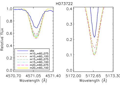
Figure 5: Mg i 4571 Å (left panel) and 5173 Å ($b_{2}$, right) observed and synthetic line profiles for the HD 73722 star. The solid thick lines are the observed profiles while the thin lines (with the same linestyle as in Fig. 3) are the synthetic profiles obtained by using the different atmospheric models described in Table 1.

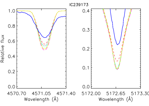
Figure 6: As in Fig. 5 for IC 2391 73.

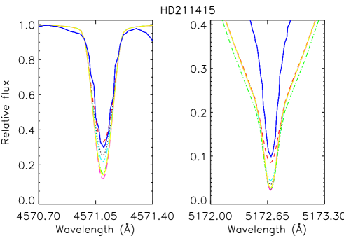
Figure 7: As in Fig. 5 for HD 211415.

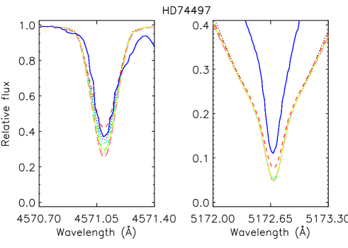
Figure 8: As in Fig. 5 for HD 74497.

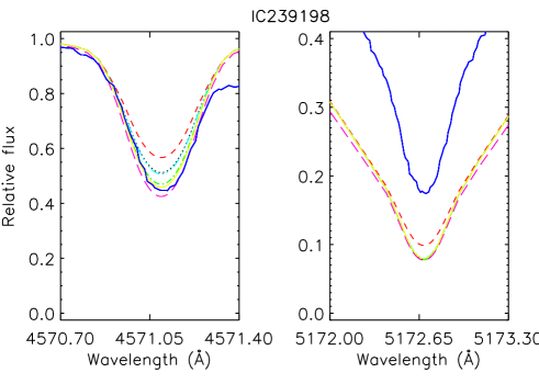
Figure 9: As in Fig. 5 for IC 2391 98.

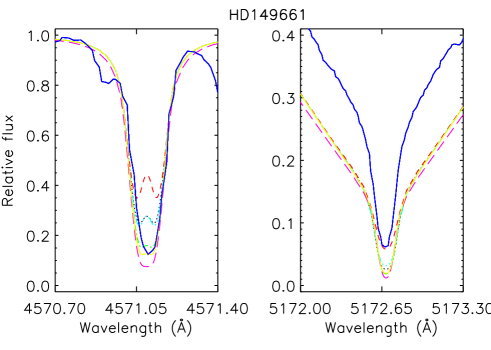
Figure 10: As in Fig. 5 for HD 149661.

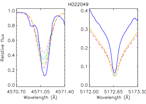
Figure 11: As in Fig. 5 for HD 22049.

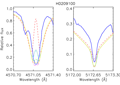
Figure 12: As in Fig. 5 for HD 209100.

As we have explained in Sec. 2.2, the most active atmospheric models are the ones with a higher value of $\log m_{0}$ and/or a steeper chromospheric temperature gradient. From Figs. 5-12, we can see that higher activity results in deeper and broader synthetic profiles. The differences between the synthetic profiles are more evident in the core of the 4571 Å line that seems very sensitive to local changes in the atmospheric model, and grow for lower $T_{\rm{eff}}$. This is in accordance with the results of Langangen et al. (2009) that found the 4571 Å line a good diagnostic of the lower chromosphere, especially for cooler atmospheres such as sunspots, where they studied this line. In particular, in Figs. 10 and 12 we can also see that a change in the degree of activity can result in a central reversal of the 4571 Å line. The models often produce a central reversal in this line that is however not observed and it appears when the formation of the line extends above the temperature minimum region, thus depending on the position of the temperature minimum in the models. Mauas et al. (1988) proposed that this reversal was a consequence of possible uncertainties in the atomic model whereas Langangen et al. (2009) and the present work show that increasing the realism in the model atom does not remove the reversal. Indeed, Langangen et al. (2009) demonstrated that this central reversal is very sensitive to the position of the chromospheric temperature rise. Our results show the same dependence of the central reversal from the the position of the chromospheric temperature rise (higher value of $\log m_{0}$ corresponding to none or less pronounced reversal), thus confirming those of Langangen et al. (2009). Moreover, we find also a dependence of the central reversal on the chromospheric temperature gradient. A steeper rise of the chromospheric temperature corresponds to more amount of emission in the line core. Therefore, on the basis of this result the observations can constrain the structure of the temperature minimum, in particular the lowest possible position of the chromospheric temperature rise and its steepest gradient. We note that the 3-D structure of the solar atmosphere could make these constraints less tight. It would be interesting to verify the sensitivity of the 4571 line to the position of the temperature minimum, using solar high spatial and temporal resolution observations of its core but to our knowledge the existing instruments do not have an adeguate spectral resolution to observe core reversals.

We are able to reproduce the Mg i 4571 Å profile for all the observed stars with a combination of $T_{\rm{eff}}$, $v\sin i$ and atmospheric model. Only for two objects, the star HD 73722 and the IC 2391 73 (Fig. 5 and 6) we cannot reproduce the observed 4571 Å line, but this could depend from the choice of the photospheric $T_{\rm{eff}}$ of the star in the atmospheric model, from the value of $v\sin i$ used for the correction or from the fact that even if we looked for stars with solar gravity and solar metallicity, these values are an approximation as we can see from Tab. 2. Indeed, the star HD 73722 shows the lowest value of $\log g$. Obviously, this comment applies to all the stars.

In Sec. 2.1, we have discussed the importance of introducing in the calculations some treatment of ultraviolet line-haze opacities. We have shown that without any correction to the MULTI background opacity, the 4571 Å line forms at lower heights in the solar atmosphere becoming less sensitive to changes at the temperature minimum. The effect of this change of formation height, in the case of the stars we are studying, results in small or not significant differences in the synthetic profiles of the 4571 Å line, obtained with different atmospheric models for the same star.

Regarding the $b_{2}$ profile, there are clear problems in reproducing the width of the line core. As we have already explained in Sec. 1, the cores of the $b$ lines form in conditions of NLTE and the populations of the lower and upper levels, involved in their formation, are determined by contributions from photons coming from atmospheric layers other than the ones in which they form. Therefore, it can be expected that local variations of the atmospheric structure do not bring large changes in the line intensities.

4 Conclusions

We analyzed the potential of four Mg i spectral lines, the 4571 Å line and the $b$ triplet, as diagnostics of chromospheric activity. Starting from the Next-Gen photospheric models, we built a grid of atmospheric models and solved the coupled equations of radiative transfer and statistical equilibrium, obtaining synthetic profiles. These profiles have been compared with observed spectra of main-sequence, solar like stars with effective temperatures $T_{\rm{eff}}=4800,5200,5600,5800,6200$ and $6400$ K, solar gravity and solar metallicity.

The comparison between the synthetic spectra and the observations is good for the Mg i 4571 Å line for stars with $T<6000$ K while there are clear problems in reproducing the width of the line core for the $b$ triplet and/or the wings. We believe that this problem could be alleviated, or even solved, by adopting for each star a photospheric model more closely matching its stellar parameters (temperature, pressure, gravity and/or metallicity). However, the grid adopted in this work (Next-Gen) is not sufficiently fine for this purpose and creating ad hoc photospheric models is outside the scope of this work.

From our analysis, we can conclude that the Mg i 4571 Å line, suggested by Langangen et al. (2009) to be a good diagnostic of the lower solar chromosphere, is significantly sensitive to changes in the activity, obtained as local changes in the atmospheric model around the minimum of temperature where the line forms, also in solar-like stars. We find the same dependency of the amount of emission in the line core of this line from the position of the chromospheric temperature rise as described by Langangen et al. (2009) and also a further dependence on the gradient of the chromospheric temperature. A lack of central reversal in the 4571 Å line gives constraint on the lowest possible position of the chromospheric temperature rise and its gradient. With this work, we also want to underline the importance of including in the Mg atomic model a correct treatment of ultraviolet line opacities. Without any correction to the MULTI background opacity, the 4571 Å line forms at lower heights and becomes less sensitive to changes in the atmospheric models and, in particular, at the temperature minimum. We verified that, for the stars we have studied in this work, without using any line blanketing treatment, the synthetic profiles of the 4571 Å line obtained with different atmospheric models for the same star, do not differ significantly.

The Mg i $b$ triplet shows instead very small and not significant response to the local atmospheric structure, in the same sample of solar-like stars selected for this work. These lines are not responsive diagnostics for atmospheric stratification.