Quantum cosmology of quadratic $f(R)$ theories with a FRW metric

Abstract

We study the quantum cosmology of a quadratic $f(R)$ theory with a FRW metric, via one of its equivalent Horndeski type actions, where the dynamics of the scalar field is induced. The classical equations of motion and the Weeler-deWitt equation, in their exact versions, are solved numerically. From the choice of a free parameter in the action follow two cases, inflation + exit and inflation alone. The numerical solution of the Wheeler-DeWitt equation depends strongly on the boundary conditions, which can be chosen so that the resulting wave function of the universe seems to be normalizable and consistent with hermitian operators.

I Introduction

Since its formulation general relativity has been a successful theory, verified in many ways and at any scale. However there are instances where it does not reproduce in a precise way the results of observations, in particular the origin of the universe and the early and present inflationary phases. One way to describe these issues have been given by means of modified gravity $f(R)$ theories. Starobisnky starobinsky has proposed $f(R)$ theory as an effective action of gravity obtained by coupling it to quantum matter fields, which explains inflation and the reheating after it and recently it has being used to explain the effects of dark matter and dark energy odintsov ; woodard , see also felice ; sotiriou ; Nojiri:2017ncd ; Nojiri:2010wj ; Nojiri:2006ri . Even if these theories appear as effective theories, one appealing feature of them is that they are pure gravity theories, although they are higher order. However, under certain conditions it is possible to give actions of Horndeski type equivalent to $f(R)$ actions langlois ; ohanlon , which have the advantage of being second order and consistently with the usual inflationary or dark energy scenarios where there are scalar fields coupled to Einstein relativity.

Another scenario where a $f(R)$ theory has been considered is the origin of the universe by a tunneling mechanism from “nothing” to the de Sitter phase of Starobinski model vilenkin . As noted in this work, at this stage a description of the universe is done in the framework of quantum cosmology, from which were computed, in the WKB approximation, the tunneling probability, and the subsequent curvature fluctuations and the duration of the inflationary phase. Quantum cosmology of $f(R)$ theories has been studied also in fr ; kenmoku ; biswas . One frequent problem related to the wave function of the universe is its interpretation and related to it, its normalizability, which might depend on the initial conditions biswas .

In this work we consider the quantum cosmology of $f(R)=R+\alpha R^{2}$ theory in the form with a scalar auxiliary field, in the FRW metric. The equations of motion in this form are second order with an additional degree of freedom, which can be eliminated, leading back to one third order equation. In the case of the Wheeler-deWitt equation, it is usual to do the Hamiltonian formulation in one of the variants with one additional degree of freedom in order to do the Hamiltonian analysis in the usual Dirac formulation. Here we use the formulation due to O’Hanlon ohanlon , with an auxiliary scalar field $\phi$, and give a numerical solution for the WdW equation in its exact form. Considering that the scale factor $a$ is positive, we require that the wave function of the universe vanishes at $a=0$, in order that the conjugate momentum of $a$ is hermitic. For the numerical computation, we consider a compact domain in $a$ and $\phi$. We get that the solution is consistent to zero on all boundaries, corresponding to normalizability. This feature persists in the noncompact limit. In the second section we make a short analysis of the classical solutions and in the third section we show the numerical solution of the WdW equation considering values of the parameter $\alpha$ for which classically the solutions are qualitatively different. In the last section we draw some conclusions.

II Lagrangian Analysis

Let us focus on the $f(R)$ model for gravity (see felice ; Nojiri:2017ncd ) without matter which has an action given by $\frac{1}{2\kappa^{2}}\int dt\sqrt{-g}f(R)$, variation with respect of the metric $g_{\mu\nu}$ results in

$$\delta A=\frac{1}{2\kappa^{2}}\int\sqrt{-g}\left[\frac{1}{2}g^{\mu\nu}F(R)+\frac{\partial f(R)}{\partial R}\frac{\delta R}{\delta g_{\mu\nu}}\right]\delta g_{\mu\nu}d^{4}x,$$

which leads to the following equations of motion

$$F(R)R_{\mu\nu}-\frac{1}{2}f(R)g_{\mu\nu}-\nabla_{\mu}\nabla_{\nu}F(R)+g_{\mu\nu}\Box F(R)=0,$$ (1)

where $F(R)=f^{\prime}(R)$.

Recalling that for a FRW geometry the metric tensor is the following

$$g_{\mu\nu}=diag\left(-N^{2},\frac{a^{2}}{1-kr^{2}},a^{2}r^{2},a^{2}r^{2}sen^{2}\theta\right),$$

then the scalar curvature is given by

$$R=\frac{6}{a^{2}}\left(\frac{a\ddot{a}}{N^{2}}+\frac{\dot{a}^{2}}{N^{2}}-\frac{a\dot{a}\dot{N}}{N^{3}}+k\right),$$

which written in terms of the Hubble factor becomes $R=12H^{2}+6\dot{H}$ once we fixed the gauge field to $N=1$ and set $k=0$. With the scalar curvature as a function of $H$, as stated above, the field equations (1) are

$$3FH^{2}=\frac{1}{2}\left(FR-f\right)-3H\dot{F},$$

$$-2F\dot{H}=\ddot{F}-H\dot{F},$$

where $F=F(H(t))$ is regarded as a scalar degree of freedon, the so called ”scalaron” $\varphi$ starobinsky .

This approach presents some calculational advantages, for instance it is evident that treating $H$ and $\varphi$ as the dynamical fields the above equations of motion are second order, choosing $a(t)$ as the dynamical variable leads to third order equations; also the dynamics of the scale factor is simply given by $a=\exp\left[\int Hdt\right]$, provided one can solve for $H(t)$. Nevertheless this statements are for one side based on setting $k=0$ and on the other side in the fixing on the gauge $N=1$. Let us examine this two conditions.

For $k\neq 0$ the curvature in terms of $H$ reads $R=12H^{2}+6\dot{H}+6k/a^{2}$. Nevertheless, this loss of generality is not a problem since the observations favor an almost ($k\approx 0$) flat universe universoplano . On the other side the choice $N(t)=1$ for the gauge field on the Lagrangian formulation represents no difficulty, however if we want to implement the Hamiltonian formulation of the theory, and thus the quantum formulation, we have to keep the gauge arbitrary. Additionally, for the Hamiltonian formulation of an $f(R)$ theory, we should implement Ostrogradsky’s formalism ostrogradsky to deal with the higher order derivatives in the Lagrangian, for instance the terms containing derivatives of the lapse function must be integrated out of the action since being a gauge field it can not have dynamics, this in turn produces third order derivatives for the scale factor and in general it is not possible to eliminate all the derivatives of $N$ as can be seen in the following Lagrangian

$$L=-\frac{24\alpha a\dddot{a}}{\dot{a}}{N^{3}+}\frac{12\alpha a\ddot{a}^{2}}{N^{3}}+\alpha\dot{a}^{2}\left(-\frac{24\ddot{a}}{N^{3}}+\frac{72k}{aN}+\frac{36a\dot{N}^{2}}{N^{5}}\right)+\frac{36\alpha\dot{a}^{4}}{aN^{3}}+\frac{36\alpha k^{2}N}{a}-\frac{6a\dot{a}^{2}}{N}+6kaN,$$

which corresponds to the quadratic Starobinsky’s model, $f(R)=R+\alpha R^{2}$. The third derivative of $a$ can be seen in the first term on the right, also we can see the presence of a derivative of $N$, which complicates the Hamiltonian formulation. These complications are avoided in the Starobinsky’s model starobinsky , with the FRW metric plugged in an O’Hanlon type of action ohanlon and given by

$$A=\frac{1}{2\kappa^{2}}\int\sqrt{-g}\left[R+\phi(\beta\phi+R)\right],$$ (2)

where $\beta$ is a free parameter. This action resembles the action used in vilenkin , where the definition of the scalar curvature is regarded as a constraint and used to eliminate $\ddot{a}$ terms in the action.

A variation with respect to $\phi$, results in $\phi=-\frac{1}{2\beta}R$ which leads to

$$A=\frac{1}{2\kappa^{2}}\int\sqrt{-g}\left(R-\frac{1}{4\beta}R^{2}\right).$$

Thus action (2) is completely equivalent to that of the Starobinsky model. Once we enter the FRW metric into this action we are able to partial integrate second order derivative terms and all the derivatives of $N$ unlike in the case mentioned above, thus we get

$$A=\frac{1}{\kappa}\int dt\left[3(1+\phi)(Nak-N^{-1}a{\dot{a}}^{2})-3N^{-1}a^{2}\dot{a}\dot{\phi}+\frac{1}{2}\beta Na^{3}\phi^{2}\right].$$

The resulting equations of motion from this action are

$$\left(6a\dot{a}^{2}+6ka\right)\left(1+\phi\right)+6a^{2}\dot{a}\dot{\phi}+\beta a^{3}\phi^{2}=0,$$ (3)

$$\left(4a\ddot{a}+2\dot{a}^{2}+2k\right)\left(1+\phi\right)+2a^{2}\ddot{\phi}+4a\dot{a}\dot{\phi}+\beta a^{2}\phi^{2}=0,$$ (4)

$$3a^{2}\ddot{a}+3a\dot{a}^{2}+3ka+\beta a^{3}\phi=0,$$ (5)

corresponding to the equation from $N$, $a$ and $\phi$, respectively, here we have fixed the gauge to $N=1$. From eq. (5) we get

$$\phi=-\frac{3}{\beta a^{2}}\left(a\ddot{a}+\dot{a}^{2}+k\right),$$ (6)

which substituted in eq. (3) gives

$$3k^{2}+\dot{a}^{2}\left(6a\ddot{a}-9\dot{a}^{2}-2\beta a^{2}-6k\right)+a^{2}\left(6\dot{a}\dddot{a}-3\ddot{a}^{2}-2k\beta\right)=0.$$ (7)

Eq. (4) is redundant.

Obviously eq. (7) can be solved only numerically. We have use the liberty to fix the free parameter $\beta$, to our advantage, in order to produce a consistent profile for the evolution of the scale factor. In general, whichever the value of $\beta$, we have an inflation stage as long as $\beta<0$, see figure 1, but for sufficiently large values (in magnitude) of $\beta$ we can see an exit of this inflationary phase, as we depict in figure 2. Also in this figure we can see that as $a$ reaches certain value its evolution stops, the universe freezes out, this feature of the model should change in the presence of matter, we are analyzing here the very reduced model since the only content of our model is gravity and the curvature scalar ”matter”.

Figure 1: Numerical profile of $a(t)$ with initial conditions $a(0)=10^{-20}$, $\dot{a}(0)=10^{-20}$, $\ddot{a}(0)=10^{-17}$, $\beta=-100$ and $k=0$.

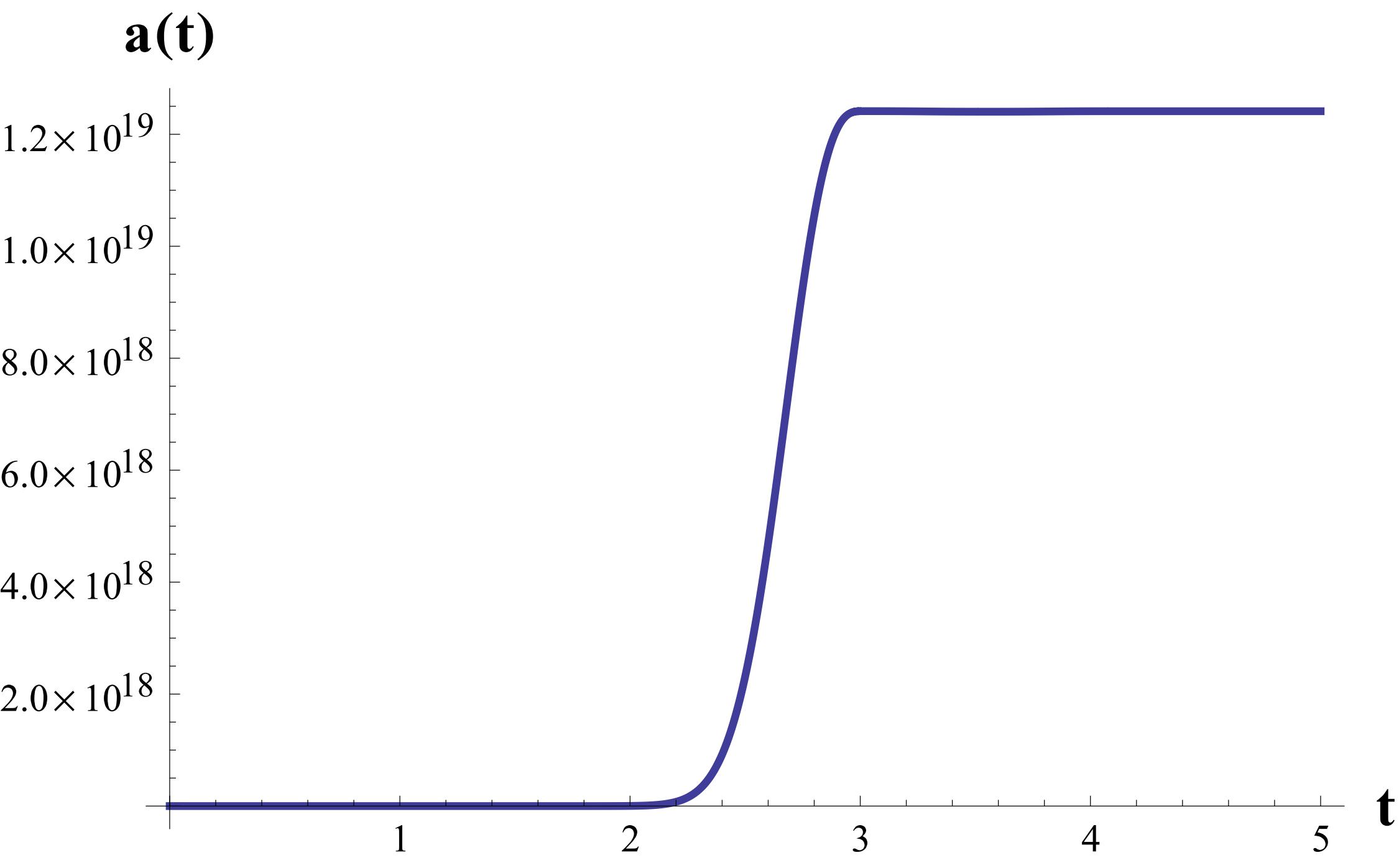
Figure 2: Numerical profile of $a(t)$ with initial conditions $a(0)=10^{-20}$, $\dot{a}(0)=10^{-20}$, $\ddot{a}(0)=10^{-17}$, $\beta=-200$ and $k=0$.

III Wheeler-deWitt equation

In this section we give the quantum formulation of this cosmological model, we begin by computing the canonical momenta of our Lagrangian, they are

$$\pi_{a} =-\left[\frac{12a\phi\dot{a}}{N}+\frac{12a\dot{a}}{N}+\frac{6a^{2}\dot{\phi}}{N}\right],$$

$$\pi_{\phi} =-\frac{6a^{2}\dot{a}}{N},$$

$$\pi_{N} =0,$$

from which, by the usual definition $H(\pi,q)=\pi_{i}q_{i}-L$, we get the customary form of the Hamiltonian as a product of a first class constraint times a Lagrange multiplier, $H=NH_{0}$, with

$$H_{0}=-6ka\phi-6ka-\beta a^{3}\phi^{2}+\frac{\phi\pi_{\phi}{}^{2}}{6a^{3}}+\frac{\pi_{\phi}{}^{2}}{6a^{3}}-\frac{\pi_{a}\pi_{\phi}}{6a^{2}}.$$ (8)

Note that besides the advantages mentioned in sec. II due to the formulation of the model based on $R$ and $\phi$ we have the usual first class constraint $H_{0}=0$ and the lagrange multiplier $N$, there is no presence of additional constraints nor we had the need to use Ostrogradky’s method or other schemes of generalized mechanics.

In the quantum version, the action of the first class constraint $H_{0}$ becomes a condition on the state wave function of the system, thus we have $\widehat{H}\psi=0$ which is the Wheeler-DeWitt equation. Therefore, we promote the classical quantities in eq. (8) to quantum operators in the coordinate representation ($q\to\widehat{q},\text{ }\pi\to-i\hbar\partial_{q}$); since the classical Hamiltonian contains terms which represent ambiguities in the quantum scheme we chose the Weyl ordering of the operators. Thus we have the non linear equation

$$\widehat{H}\psi=\left[-\hbar^{2}\left(\phi+1\right)\frac{\partial^{2}}{\partial\phi^{2}}+a\hbar^{2}\frac{\partial^{2}}{\partial\phi\partial a}-2\hbar^{2}\frac{\partial}{\partial\phi}-6\beta a^{6}\phi^{2}-36ka^{4}\left(\phi+1\right)\right]\psi=0.$$ (9)

We solve this numerically and as can be seen from the profile of $\psi^{2}$ depicted in figures (3,4) the model produces a normalizable wave function of the universe whether we deal with values of $\beta$ producing an exit of the inflationary phase or not, in the classical scheme of the previous section; this means that in principle the model could predict both cases from the quantum version. Note that we have set $\psi(a=0,\phi)=0$ as an initial boundary condition to ensure the hermiticity of the quantum operators as explained in kuchar considering that $a\geq 0$. Also we have set $\psi(a,\phi_{0})=f(a)$ on the $\phi$-boundaries, this is a good condition in order to prevent the numerical solution to be identically zero; conditions of the type $\partial_{\phi}\psi(a,\pm\phi_{0})=0$ restrict to strong the wave function so that it can not evolve from the zero value on the $a=0$ boundary. Moreover, we can see that the non-vanishing values of $\psi$ are grouped in a well defined region of the domain, which ensures that the wave function is normalizable. Assuming that the universe originates in a very small value of $a$ this wave function points to a fast grow of the universe to the values where this wave function has it’s maximum, pointing to the existence of a inflationary phase.

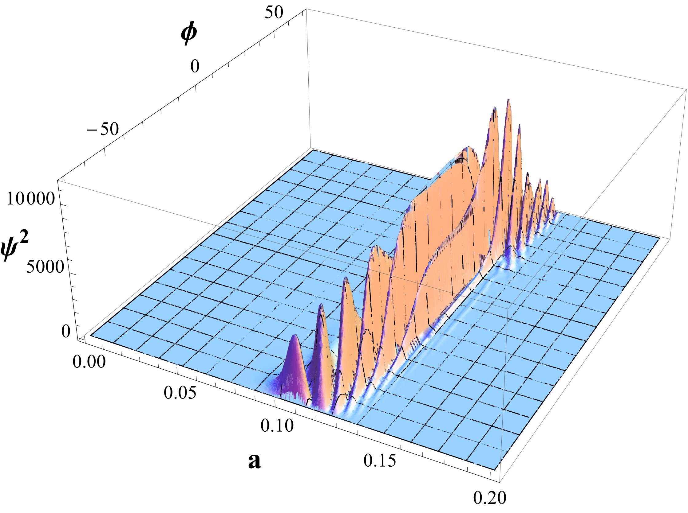
Figure 3: Numerical profile of $\psi(a,\phi)$ with initial conditions: $\psi(0,\phi)=0$ and $\psi(a,\phi_{0})=f(a)$, where $\phi_{0}$ defines half the with of our solution domain over $\phi$. Here we have set $\hbar=1$, $\beta=-200$ and $k=0$.

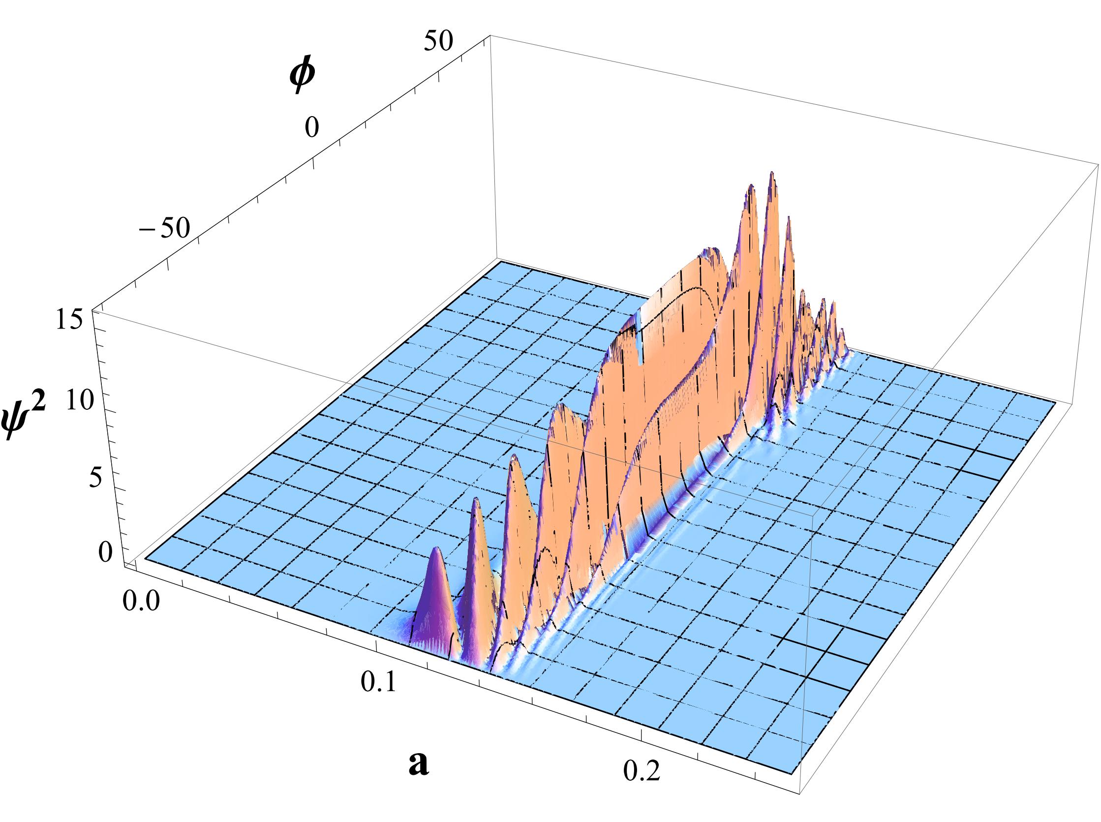
Figure 4: Numerical profile of $\psi(a,\phi)$ with initial conditions: $\psi(0,\phi)=0$ and $\psi(a,\phi_{0})=f(a)$, where $\phi_{0}$ defines half the with of our solution domain over $\phi$. Here we have set $\hbar=1$, $\beta=-100$ and $k=0$.

The statement concerning the normalization of the wave function, although motivated by the figures above, can be analytically justified if at least on the upper and lower limits of the numerical domain one could find hints that the boundary conditions we establish hold in certain degree, with the only assumption that the wave function is $C^{2}$-class. We attack this by proposing a series solution to the Wheeler-DeWitt equation given by

$$\psi={\displaystyle\sum\limits_{n=0}^{\infty}}f_{n}(\phi)a^{n},$$ (10)

once entered in (8) result in a system of differential equations for the coefficients $f_{n}(\phi)$

$$\left(1+\phi\right)f_{0}^{\prime\prime}+2f_{0}^{\prime} =0$$

$$\left(1+\phi\right)f_{1}^{\prime\prime}+f_{1}^{\prime} =0$$

$$f_{2}^{\prime\prime} =0$$

$$\left(1+\phi\right)f_{3}^{\prime\prime}+f_{3}^{\prime} =0$$

$$\left(1+\phi\right)f_{4}^{\prime\prime}-2f_{4}^{\prime}+36k\left(1+\phi\right)f_{0} =0$$

$$\vdots$$

which can be analytically solved starting from $f_{0}$ and up to the desired $n$-coefficient, resulting in

$$f_{0} =c_{2}-\frac{c_{1}}{\phi+1},$$

$$f_{1} =c_{3}\log(\phi+1)+c_{4},$$

$$f_{2} =c_{5}\phi+c_{4},$$

$$f_{3} =c_{5}\left(\frac{\phi^{2}}{2}+\phi\right)+c_{6}$$

$$f_{4} =\frac{18c_{2}k\phi^{2}}{\hbar^{2}}+\frac{36c_{2}k\phi}{\hbar^{2}}-\frac{18c_{1}k\phi}{\hbar^{2}}+\frac{c_{6}\phi^{3}}{3}+c_{6}\phi^{2}+c_{6}\phi+c_{7}$$

$$\vdots$$

The free parameters $c_{n}$ can be fixed according to the boundary conditions on the wave function, to ensure that $\psi(0,\phi)=0$ we must have $c_{1}=c_{2}=0$, we also set $c_{3}=0$ in order to prevent the presence of the term $\log(1+\phi)$, the rest of these constants remain unconstraint, we set $c_{n}=(-1)^{n}/n!$, with these one can see that around $a=0$ the wave function converges to zero. In the same way one can calculate the same series solution around $a=\infty$ which results in the trivial solution, all the coefficients are identically zero. This can be easily seen from the corresponding Wheeler-DeWitt equation

$$\left[\hbar^{2}b^{6}\left(1+\phi\right)\frac{\partial^{2}}{\partial\phi^{2}}+\hbar^{2}b^{7}\frac{\partial^{2}}{\partial\phi\partial b}+2b^{6}\hbar^{2}\frac{\partial}{\partial\phi}+36b^{2}k\left(1\text{$+$}\phi\right)\text{$+$}6\beta\phi^{2}\right]\psi=0,$$

where $b=1/a$, which at $b=0$ gives $\psi=0$.

Also we can see from eq. (8) that as $\phi\to\infty$ the $\phi^{2}$ term dominates, forcing the wave function to be zero in this limit and then allowing the integrability over $\phi$. Thus, we can say that the function is normalizable since being a soft surface it must reach a finite maximum and then take on zero values asymptotically as $a\to 0$ and $a\to\infty$.

IV Conclusions

We have studied the classical and quantum formulation of a $f(R)$ modified theory of General Relativity based on the Starobinsky model, with a scalar field in a Horndeski type action, in a cosmological setting with a FRW metric. Thus the lagrangian and hamiltonian formulations are straightforward. We consider the numerical solutions for the exact equations in both scenarios, classical and quantum, taking a compact domain for the numerical computation. Although the dependence of the classical solutions on the parameter $\alpha$ can change their topology, the corresponding solutions of the WdW equation do not show such a difference. In fact, for suitable boundary conditions, these solutions tend to zero at the boundaries, pointing to normalizability of the wave function, consistently with the probabilistic interpretation. The form of the wave function suggests that this case could be interpreted by a conditional probability as in susyfrw , where the scalar field plays the role of time.

References

- (1) A.A. Starobinsky, A new type of isotropic cosmological models without singularity, Phys. Lett. B, 91 (1980) 99-102.
- (2) S. Nojiri and S.D. Odintsov, Modified gravity with negative and positive powers of the curvature: Unification of the inflation and of the cosmic acceleration, Phys. Rev. D 68, 123512 (2003), [hep-th/0307288].
- (3) R. P. Woodard, Avoiding dark energy with 1/r modifications of gravity, Lect. Notes Phys. 720, 403 (2007), [astro-ph/0601672].
- (4) A. De Felice and S. Tsujikawa, Theories, Living Rev. Relativity, 13 (2010) 3.
- (5) T.P. Sotiriou and V. Faraoni, f(R) Theories Of Gravity, Rev. Mod. Phys. 82, 451 (2010), [arXiv:0805.1726 [gr-qc]].
- (6) S. Nojiri, S.D. Odintsov and V.K.Oikonomou, Modified Gravity Theories on a Nutshell: Inflation, Bounce and Late-time Evolution, [arXiv:1705.11098 [gr-qc]].
- (7) S. Nojiri and S.D. Odintsov, Unified cosmic history in modified gravity: from F(R) theory to Lorentz non-invariant models, Phys. Rept. 505 (2011) 59. doi:10.1016/j.physrep.2011.04.001 [arXiv:1011.0544 [gr-qc]].
- (8) S. Nojiri and S.D. Odintsov, Introduction to modified gravity and gravitational alternative for dark energy, eConf C 0602061 (2006) 06 Int. J. Geom. Meth. Mod. Phys. 4 (2007) 115 doi:10.1142/S0219887807001928 [hep-th/0601213].
- (9) J. O’Hanlon, Intermediate-Range Gravity: A Generally Covariant Model, Phys. Rev. Lett. 29 (1972) 137.
- (10) D. Langlois and K. Noui, Degenerate higher derivative theories beyond Horndeski: evading the Ostrogradski instability, J. Cosmol. Astropart. Phys. 02 (2016) 034.
- (11) A. Vilenkin, Classical and quantum cosmology of the Starobinsky inflationary model, Phys. Rev. D. 32 (1985) 2511-2521.
- (12) S. Biswas, A. Shaw and B. Modak, “Decoherence in the Starobinsky Model”, Gen. Rel. Grav. 31 (1999) 1015.
- (13) M.B. Mijic, M.S. Morris and W. Suen, “Initial conditions for R +eR cosmology”, Phys. Rev. D39 (1989) 1496; H. van Elst, J. E. Lidsey and R. Tavakol, “Quantum cosmology and higher-order Lagrangian theories”, Class. Quantum Grav. 11 (1994) 248.
- (14) M. Kenmoku et al., Classical and quantum solutions and the problem of time in cosmology, Class. Quantum Grav., 13 (1996) 1751-1759.
- (15) L. Anderson, et al., The clustering of galaxies in the SDSS-III Baryon Oscillation Spectroscopic Survey: baryon acoustic oscillations in the Data Releases 10 and 11 Galaxy samples, Mon. Not. R. Astron. Soc., 441 (2014) 24-62.
- (16) M.V. Ostrogradsky, Memoires sur les equations differentielles relatives au probleme des isoperimetres, Mem. Acad. St. Petersburg, 6 (1850) 385. C. Grosse-Knetter, Effective Lagriangians with higher derivatives and equations of motion, Phys. Rev. D, 49 (1994) 6709-6719. T. Chen, et al., Higher derivative theories with constraints: exorcising Ostrogradsky’s ghost, JCAP02 (2013) 042.
- (17) G. Horowitz, Quantum cosmology with a positive-definite action, Phys. Rev. D 31 (1985) 1169.
- (18) K.V. Kuchař, Time and interpretations of quantum gravity, in Proceedings of the 4th Canadian Conference on General Relativity and Relativistic Astrophysics, edited by G. Kunstatter, D. Vincent, and J. Williams (World Scientific, Singapore, 1992); Int. J. Mod. Phys. D 20 (2011) 3.
- (19) C. Ramírez and V. Vázquez-Báez, Quantum supersymmetric FRW cosmology with a scalar field, Phys. Rev. D 93 (2016) 043505.