On the risk of convex-constrained least squares estimators under misspecification

Abstract

We consider the problem of estimating the mean of a noisy vector. When the mean lies in a convex constraint set, the least squares projection of the random vector onto the set is a natural estimator. Properties of the risk of this estimator, such as its asymptotic behavior as the noise tends to zero, have been well studied. We instead study the behavior of this estimator under misspecification, that is, without the assumption that the mean lies in the constraint set. For appropriately defined notions of risk in the misspecified setting, we prove a generalization of a low noise characterization of the risk due to Oymak and Hassibi [7] in the case of a polyhedral constraint set. An interesting consequence of our results is that the risk can be much smaller in the misspecified setting than in the well-specified setting. We also discuss consequences of our result for isotonic regression.

1 Introduction

In many statistical problems, it is common to model the observations $y_{1},\dots,y_{n}\in{\mathbb{R}}$ as $y_{i}=\theta^{*}_{i}+\sigma z_{i}$ where $\theta_{1}^{*},\dots,\theta_{n}^{*}$ are unknown parameters of interest, $z_{1},\dots,z_{n}$ represent noise or error variables that have mean zero, and $\sigma>0$ denotes a scale parameter. In vector notation, this is equivalent to writing

$$Y=\theta^{*}+\sigma Z,$$ (1)

where $Y\coloneqq(y_{1},\dots,y_{n})$, $\theta^{*}\coloneqq(\theta^{*}_{1},\dots,\theta^{*}_{n})$, and $Z\coloneqq(z_{1},\ldots,z_{n})$. A common instance of this model is the Gaussian sequence model, where the $z_{1},\dots,z_{n}$ are independent standard Gaussian random variables, in which case the model can be written as $Y\sim N(\theta^{*},\sigma^{2}I_{n})$, where $I_{n}$ is the $n\times n$ identity matrix.

A standard method of estimating $\theta^{*}$ from the observation vector $Y$ is to fix a closed convex set ${\mathcal{C}}$ of ${\mathbb{R}}^{n}$ and use the least squares estimator under the constraint given by $\theta\in{\mathcal{C}}$. Specifically, the least squares projection is

$$\Pi_{{\mathcal{C}}}(x)\coloneqq\mathop{\rm argmin}_{\theta\in{\mathcal{C}}}\|x-\theta\|^{2},$$ (2)

(where $\|\cdot\|$ denotes the standard Euclidean norm in ${\mathbb{R}}^{n}$), and one estimates $\theta^{*}$ by

$$\hat{\theta}(Y)\coloneqq\Pi_{{\mathcal{C}}}(Y).$$ (3)

When ${\mathcal{C}}$ is taken to be $\{X\beta:\|\beta\|_{1}\leq R\}$ for some deterministic $n\times p$ matrix $X$ and $R>0$, this estimator becomes LASSO in the constrained form as originally proposed by Tibshirani [10]. When ${\mathcal{C}}$ is taken to be $\{X\beta:\min_{j}\beta_{j}\geq 0\}$, this estimator becomes nonnegative least squares. Note that shape restricted regression estimators are special cases of nonnegative least squares for appropriate choices of $X$ (see, for example, Groeneboom and Jongbloed [4]). Also, note that both sets $\{X\beta:\|\beta\|_{1}\leq R\}$ and $\{X\beta:\min_{j}\beta_{j}\geq 0\}$ are examples of polyhedral sets. Therefore in most applications, the constraint set ${\mathcal{C}}$ is polyhedral.

There exist many results in the literature studying the accuracy of $\hat{\theta}(Y)$ as an estimator for $\theta^{*}$. Most of these results make the assumption that $\theta^{*}\in{\mathcal{C}}$. In this paper, we shall refer to this assumption as the well-specified assumption. Essentially, the constraint set ${\mathcal{C}}$ can be taken to be a part of the model specification, and the assumption $\theta^{*}\in{\mathcal{C}}$ means that the true mean vector $\theta^{*}$ satisfies the model assumptions, i.e. the model is well-specified.

Under the well-specified assumption, it is reasonable and common to measure the accuracy of $\hat{\theta}(Y)$ via its risk under squared Euclidean distance. More precisely, the risk of $\hat{\theta}(Y)$ is defined by

$$R(\hat{\theta},\theta^{*})\coloneqq{\mathbb{E}}_{\theta^{*}}\|\hat{\theta}(Y)-\theta^{*}\|^{2}$$

where ${\mathbb{E}}_{\theta^{*}}$ refers to expectation taken with respect to the noise $Z$ in the model $Y=\theta^{*}+\sigma Z$.

Many results on $R(\hat{\theta},\theta^{*})$ in the well-specified setting are available in the literature. Of all the available results, let us isolate two results from Oymak and Hassibi [7] because of their generality. In the setting where $Z\sim N(0,I_{n})$, Oymak and Hassibi [7] first proved the upper bound

$$\frac{1}{\sigma^{2}}R(\hat{\theta},\theta^{*})\leq\delta(T_{{\mathcal{C}}}(\theta^{*})),$$ (4)

where $T_{\mathcal{C}}(\theta^{*})$ denotes the tangent cone of ${\mathcal{C}}$ at $\theta^{*}$, defined by

$$T_{{\mathcal{C}}}(\theta^{*})=\operatorname{cl}\left\{\alpha(\theta-\theta^{*}):\alpha\geq 0,\theta\in{\mathcal{C}}\right\},$$ (5)

(“$\operatorname{cl}$” denotes closure), and where $\delta\left(T_{{\mathcal{C}}}(\theta^{*})\right)$ denotes the statistical dimension of the cone $T_{{\mathcal{C}}}(\theta^{*})$. In general, the statistical dimension of a closed cone $T\subseteq{\mathbb{R}}^{n}$ is defined as

$$\delta(T)\coloneqq{\mathbb{E}}\|\Pi_{T}(Z)\|^{2},$$ (6)

where the expectation is with respect to $Z\sim N(0,I_{n})$. Many properties of the statistical dimension are covered by Amelunxen et al. [2].

In the case when the constraint set ${\mathcal{C}}$ is a subspace, the estimator $\hat{\theta}(Y)$ is linear and, in this case, it is easy to see that $\delta(T_{{\mathcal{C}}}(\theta^{*}))$ is simply the dimension of ${\mathcal{C}}$, so that inequality (4) becomes an equality. For general closed convex sets, it is therefore reasonable to ask how tight inequality (4) is. It is not hard to construct examples of ${\mathcal{C}}$ and $\theta^{*}\in{\mathcal{C}}$ where inequality (4) is loose for fixed $\sigma>0$. However Oymak and Hassibi [7] proved remarkably that the upper bound in (4) is tight in the limit as $\sigma\downarrow 0$ (we shall refer to this in the sequel as the low $\sigma$ limit); that is, when $Z\sim N(0,I_{n})$,

$$\lim_{\sigma\downarrow 0}\frac{1}{\sigma^{2}}R(\hat{\theta},\theta^{*})=\delta(T_{{\mathcal{C}}}(\theta^{*})).$$ (7)

In summary, Oymak and Hassibi [7] proved that $\sigma^{2}\delta(T_{{\mathcal{C}}}(\theta^{*}))$ is a nice formula for the risk of $\hat{\theta}(Y)$ that is, in general, an upper bound which is tight in the low $\sigma$ limit.

We remark that although Oymak and Hassibi [7] state the results (4) and (7) for the specific case $Z\sim N(0,I_{n})$, their proof automatically extends to the more general setting where $Z$ is an arbitrary zero mean random vector with ${\mathbb{E}}\|Z\|^{2}<\infty$ (the components $Z_{1},\dots,Z_{n}$ of $Z$ can be arbitrarily dependent), provided we generalize the definition (6) of statistical dimension by taking the expectation with respect to $Z$, without assuming $Z$ is standard Gaussian. We refer to this modification of the definition (6) as the generalized statistical dimension of the cone $T$. As a slight abuse of notation, we use the same notation $\delta(\cdot)$ for this more general concept, with the understanding that the expectation in the definition is with respect to the distribution of $Z$. By dropping the Gaussian assumption, the generalized statistical dimension loses much of the interpretability and nice geometric properties of the usual statistical dimension [2], but still serves as an abstract notion of the size of a cone $T$ with respect to a distribution $Z$.

This paper deals with the behavior of the estimator $\hat{\theta}(Y)$ when the assumption $\theta^{*}\in{\mathcal{C}}$ is violated. We shall refer to the situation when $\theta^{*}\notin{\mathcal{C}}$ as the misspecified setting. Note that, in practice, one can never know if the unknown $\theta^{*}$ truly lies in ${\mathcal{C}}$. It is therefore necessary to study the behavior of $\hat{\theta}(Y)$ under misspecification.

For the misspecified setting, one must first note that it is no longer reasonable to measure the performance of $\hat{\theta}(Y)$ by the risk $R(\hat{\theta},\theta^{*})$, simply because $\hat{\theta}(Y)$ is constrained to be in ${\mathcal{C}}$ and hence cannot be expected to be close to $\theta^{*}$ which is essentially unconstrained. There are two natural notions of accuracy of $\hat{\theta}(Y)$ in the misspecified setting, which we call the misspecified risk and the excess risk. The misspecified risk is defined as

$$M(\hat{\theta},\theta^{*})\coloneqq{\mathbb{E}}_{\theta^{*}}\|\hat{\theta}(Y)-\Pi_{{\mathcal{C}}}(\theta^{*})\|^{2},$$ (8)

and the excess risk is defined as

$$E(\hat{\theta},\theta^{*})\coloneqq{\mathbb{E}}_{\theta^{*}}\|\hat{\theta}(Y)-\theta^{*}\|^{2}-\|\Pi_{{\mathcal{C}}}(\theta^{*})-\theta^{*}\|^{2}.$$ (9)

The misspecified risk, $M(\hat{\theta},\theta^{*})$, is motivated by the observation that, in the misspecifed case, the estimator $\hat{\theta}(Y)$ is really estimating $\Pi_{{\mathcal{C}}}(\theta^{*})$ so it is natural to measure its squared distance from $\Pi_{{\mathcal{C}}}(\theta^{*})$. On the other hand, the excess risk, $E(\hat{\theta},\theta^{*})$, measures the squared distance of the estimator from $\theta^{*}$ relative to the squared distance of $\Pi_{{\mathcal{C}}}(\theta^{*})$ from $\theta^{*}$. We refer the reader to Bellec [3] and Section 2 for some background and basic properties on these notions of accuracy under misspecification. For example, it can be shown that $M(\hat{\theta},\theta^{*})$ is always less than or equal to $E(\hat{\theta},\theta^{*})$ (see (17)). It is easy to see that both of these risk measures equal $R(\hat{\theta},\theta^{*})$ in the well-specifed case i.e.,

$$R(\hat{\theta},\theta^{*})=M(\hat{\theta},\theta^{*})=E(\hat{\theta},\theta^{*}),\qquad\text{when $\theta^{*}\in{\mathcal{C}}$}.$$ (10)

An analogue to inequality (4) for the case of misspecification has been proved by Bellec [3, Corollary 2.2], who showed that

$$\frac{1}{\sigma^{2}}M(\hat{\theta},\theta^{*})\leq\frac{1}{\sigma^{2}}E(\hat{\theta},\theta^{*})\leq\delta(T_{{\mathcal{C}}}(\Pi_{{\mathcal{C}}}(\theta^{*}))).$$ (11)

Again, although this was originally stated for $Z\sim N(0,I_{n})$, it holds for arbitrary zero mean random vectors $Z$ with ${\mathbb{E}}\|Z\|^{2}<\infty$. Note the similarity between the right-hand sides of the inequalities (4) and (11). The only difference is that the tangent cone at $\theta^{*}$ is replaced by the tangent cone at $\Pi_{{\mathcal{C}}}(\theta^{*})$ in the case of misspecification. Moreover, in the well-specified setting, the above inequality (11) reduces to (4).

It is now very natural to ask if the second inequality in (11) is tight in the low $\sigma$ limit. One might guess that this should be the case given the result (7) for the well-specified setting. However, it turns out that (11) is not sharp in the low $\sigma$ limit. The main contribution of this paper is to provide an exact formula for the low $\sigma$ limit of $M(\hat{\theta},\theta^{*})$ and $E(\hat{\theta},\theta^{*})$ when ${\mathcal{C}}$ is polyhedral. Specifically, in Theorem 3.1, we prove that if the noise $Z$ is zero mean with ${\mathbb{E}}\|Z\|^{2}<\infty$ and if ${\mathcal{C}}$ is polyhedral, then

$$\lim_{\sigma\downarrow 0}\frac{1}{\sigma^{2}}M(\hat{\theta},\theta^{*})=\lim_{\sigma\downarrow 0}\frac{1}{\sigma^{2}}E(\hat{\theta},\theta^{*})=\delta\left(T_{{\mathcal{C}}}(\Pi_{{\mathcal{C}}}(\theta^{*}))\cap(\theta^{*}-\Pi_{{\mathcal{C}}}(\theta^{*}))^{\perp}\right),$$ (12)

where $v^{\perp}\coloneqq\{u\in{\mathbb{R}}^{n}:\left<u,v\right>=0\}$ for vectors $v\in{\mathbb{R}}^{n}$. As we remarked earlier, in most applications, the constraint set ${\mathcal{C}}$ is polyhedral.

Because the set $T_{{\mathcal{C}}}(\Pi_{{\mathcal{C}}}(\theta^{*}))\cap(\theta^{*}-\Pi_{{\mathcal{C}}}(\theta^{*}))^{\perp}$ is a subset of $T_{{\mathcal{C}}}(\Pi_{{\mathcal{C}}}(\theta^{*}))$, the right hand side of (12) is never larger than $\delta(T_{{\mathcal{C}}}(\Pi_{{\mathcal{C}}}(\theta^{*})))$. Under the assumption that the polyhedron ${\mathcal{C}}$ has a nonempty interior along with a mild condition on the noise $Z$, it can be proved that the right hand side of (12) is strictly smaller than $\delta(T_{{\mathcal{C}}}(\Pi_{{\mathcal{C}}}(\theta^{*})))$ when $\theta^{*}\notin{\mathcal{C}}$ (an even stronger statement is proved in 3.4), which then implies that $\lim_{\sigma\downarrow 0}\sigma^{-2}M(\hat{\theta},\theta^{*})<\lim_{\sigma\downarrow 0}\sigma^{-2}R(\hat{\theta},\Pi_{{\mathcal{C}}}(\theta^{*}))$. This inequality is more interpretable in the following form:

$$\lim_{\sigma\downarrow 0}\frac{1}{\sigma^{2}}{\mathbb{E}}_{\theta^{*}}\|\hat{\theta}(Y)-\Pi_{{\mathcal{C}}}(\theta^{*})\|^{2}<\lim_{\sigma\downarrow 0}\frac{1}{\sigma^{2}}{\mathbb{E}}_{\Pi_{{\mathcal{C}}}(\theta^{*})}\|\hat{\theta}(Y)-\Pi_{{\mathcal{C}}}(\theta^{*})\|^{2}\qquad\text{whenever $\theta^{*}\notin{\mathcal{C}}$}.$$ (13)

Inequality (13) can be qualitatively understood as follows. The left hand side above corresponds to misspecification where the data are generated from $\theta^{*}\notin{\mathcal{C}}$ while the right hand side corresponds to the well-specified setting where the data are generated from $\Pi_{{\mathcal{C}}}(\theta^{*})$. Note that in both cases, the estimator $\hat{\theta}(Y)$ is really estimating $\Pi_{{\mathcal{C}}}(\theta^{*})$ so it is natural to compare the squared expected distance to $\Pi_{{\mathcal{C}}}(\theta^{*})$ in both situations. The interesting aspect is that (in the low $\sigma$ limit) the expected squared distance is smaller in the misspecified setting compared to the well-specified setting. To the best of our knowledge, this fact has not been noted in the literature previously at this level of generality.

Our main result, Theorem 3.1, is stated and proved in Section 3 where some intuition is also provided for the exact form of the low $\sigma$ limit in misspecification. The low $\sigma$ limit can be explicitly computed in certain specific situations. In Section 4, we specialize to the Gaussian model $Z\sim N(0,I_{n})$ and study in detail the examples when ${\mathcal{C}}$ is the nonnegative orthant and when ${\mathcal{C}}$ is the monotone cone (this latter case corresponds to isotonic regression).

In Section 5, we explore issues naturally related to Theorem 3.1. In Section 5.1, we consider the situation when ${\mathcal{C}}$ is not polyhedral. It seems hard to characterize the low $\sigma$ misspecification limits in this case but it is possible to compute them when ${\mathcal{C}}$ is the unit ball. It is interesting to note that the low $\sigma$ limits of $M(\hat{\theta},\theta^{*})$ and $E(\hat{\theta},\theta^{*})$ are different in this case (in sharp contrast to the polyhedral situation). In Section 5.2, we deal with the risks when $\sigma$ is large. Under some conditions, it is possible to write a formula for the large $\sigma$ limits of $M(\hat{\theta},\theta^{*})$ and $E(\hat{\theta},\theta^{*})$; see 5.3. In Section 5.3, we deal with the maximum normalized risks:

$$\sup_{\sigma>0}\frac{1}{\sigma^{2}}M(\hat{\theta},\theta^{*})\quad\text{ and }\quad\sup_{\sigma>0}\frac{1}{\sigma^{2}}E(\hat{\theta},\theta^{*}).$$ (14)

In the well-specified setting, inequalities (4) and (7) together imply that the maximum normalized risk equals $\delta(T_{{\mathcal{C}}}(\theta^{*}))$. However in the misspecified setting, the quantities (14) lie between $\delta(T_{{\mathcal{C}}}(\Pi_{{\mathcal{C}}}(\theta^{*}))\cap(\theta^{*}-\Pi_{{\mathcal{C}}}(\theta^{*}))^{\perp})$ and $\delta(T_{{\mathcal{C}}}(\Pi_{{\mathcal{C}}}(\theta^{*})))$. It seems hard to write down an exact formula for the quantities (14) but we present some simulation evidence in Section 5.3 to argue that they can be strictly between $\delta(T_{{\mathcal{C}}}(\Pi_{{\mathcal{C}}}(\theta^{*}))\cap(\theta^{*}-\Pi_{{\mathcal{C}}}(\theta^{*}))^{\perp})$ and $\delta(T_{{\mathcal{C}}}(\Pi_{{\mathcal{C}}}(\theta^{*})))$.

We conclude with an appendix that contains technical lemmas and proofs of the various intermediate results throughout the paper.

2 Background and Notation

In this short section, we shall set up some notation and also recollect standard results in convex analysis that will be used in the remainder of the paper.

For $x\in{\mathbb{R}}^{n}$ and $r>0$, we denote by $B_{r}(x)\coloneqq\{u\in{\mathbb{R}}^{n}:\|u-x\|\leq r\}$ the closed ball of radius $r$ centered at $x$. For $v\in{\mathbb{R}}^{n}$, let $v^{\perp}\coloneqq\{u\in{\mathbb{R}}^{n}:\langle u,v\rangle=0\}$ denote the hyperplane with normal vector $v$. For $\theta_{0}\in{\mathcal{C}}$, let $F_{\mathcal{C}}(\theta_{0})\coloneqq\{\theta-\theta_{0}:\theta\in{\mathcal{C}}\}$ be the result of re-centering the set ${\mathcal{C}}$ about $\theta_{0}$. Also recall the definition of the tangent cone (5) and note that $T_{\mathcal{C}}(\theta_{0})=\operatorname{cl}\{\alpha x:x\in F_{\mathcal{C}}(\theta_{0}),\alpha>0\}$.

If $A$ is an $m\times n$ matrix and $J\subseteq\{1,\ldots,m\}$, we let $a_{j}$ denote the $j$th row of $A$, and let $A_{J}$ denote the matrix obtained by combining the rows of $A$ indexed by $J$.

A polyhedron refers to a set of the form $\{x\in{\mathbb{R}}^{n}:Ax\leq b\}$ for some $A\in{\mathbb{R}}^{m\times n}$ and $b\in{\mathbb{R}}^{n}$ where the inequality $\leq$ is interpreted coordinate-wise, i.e. $\langle a_{j},x\rangle\leq b_{j}$ for $j=1,\ldots,m$. We will assume that no two pairs $(a_{j},b_{j})$ and $(a_{k},b_{k})$ are scalar multiples of each other. A polyhedral cone is a set of the form $\{x\in{\mathbb{R}}^{n}:Ax\leq 0\}$ for some $A\in{\mathbb{R}}^{m\times n}$. Again, we will assume that no two rows of $A$ are scalar multiples of each other. A face of a polyhedron refers to any subset obtained by setting some of the polyhedron’s linear inequality constraints to equality instead.

In the remainder of this section, we shall collect some standard results above convex projections that will be used in the paper. These results can be found in a standard reference such as [5]. Recall that $\Pi_{{\mathcal{C}}}(x)$ denotes the projection of a vector $x\in{\mathbb{R}}^{n}$ on a closed convex set ${\mathcal{C}}$. It is well known that $\Pi_{\mathcal{C}}(x)$ is the unique vector in ${\mathcal{C}}$ satisfying the optimality condition

$$\langle z-\Pi_{\mathcal{C}}(x),x-\Pi_{\mathcal{C}}(x)\rangle\leq 0,\qquad\forall z\in{\mathcal{C}}.$$ (15)

Consequently, we have the following Pythagorean inequality

$$\|z-x\|^{2}=\|z-\Pi_{\mathcal{C}}(x)\|^{2}+\|\Pi_{\mathcal{C}}(x)-x\|^{2}+2\langle z-\Pi_{\mathcal{C}}(x),\Pi_{\mathcal{C}}(x)-x\rangle\geq\|z-\Pi_{\mathcal{C}}(x)\|^{2}+\|\Pi_{\mathcal{C}}(x)-x\|^{2}.$$ (16)

Plugging in $z=\Pi_{\mathcal{C}}(y)$ and $x=\theta^{*}$ shows that the misspecified error is upper bounded by the excess error, that is,

$$\|\Pi_{\mathcal{C}}(y)-\Pi_{\mathcal{C}}(\theta^{*})\|^{2}\leq\|\Pi_{\mathcal{C}}(y)-\theta^{*}\|^{2}-\|\Pi_{\mathcal{C}}(\theta^{*})-\theta^{*}\|^{2},\qquad\forall y\in{\mathbb{R}}^{n}.$$ (17)

If instead we plug in $z=\Pi_{\mathcal{C}}(\theta^{*})$ to (15), we have $\langle\Pi_{\mathcal{C}}(x)-\Pi_{\mathcal{C}}(\theta^{*}),x-\Pi_{\mathcal{C}}(x)\rangle\geq 0$, which implies

$$\|\Pi_{\mathcal{C}}(x)-\theta^{*}\|^{2}-\|\Pi_{\mathcal{C}}(\theta^{*})-\theta^{*}\|^{2} =-\|\Pi_{\mathcal{C}}(x)-\Pi_{\mathcal{C}}(\theta^{*})\|^{2}+2\langle\Pi_{\mathcal{C}}(x)-\Pi_{\mathcal{C}}(\theta^{*}),\Pi_{\mathcal{C}}(x)-\theta^{*}\rangle$$ (18)

$$\leq-\|\Pi_{\mathcal{C}}(x)-\Pi_{\mathcal{C}}(\theta^{*})\|^{2}+2\langle\Pi_{\mathcal{C}}(x)-\Pi_{\mathcal{C}}(\theta^{*}),x-\theta^{*}\rangle$$ (19)

$$\leq\|x-\theta^{*}\|^{2}.$$ (20)

Combining this with (17), we see that for $Y=\theta^{*}+\sigma Z$ we have

$$0\leq\|\Pi_{\mathcal{C}}(Y)-\Pi_{\mathcal{C}}(\theta^{*})\|^{2}\leq\|\Pi_{\mathcal{C}}(Y)-\theta^{*}\|^{2}-\|\Pi_{\mathcal{C}}(\theta^{*})-\theta^{*}\|^{2}\leq\sigma^{2}\|Z\|^{2}.$$ (21)

In the special case where ${\mathcal{C}}$ is a cone, the optimality condition (15) implies that $\Pi_{\mathcal{C}}(x)$ is the unique vector in ${\mathcal{C}}$ satisfying

$$\langle\Pi_{\mathcal{C}}(x),x-\Pi_{\mathcal{C}}(x)\rangle=0,\quad\text{ and }\quad\langle z,x-\Pi_{\mathcal{C}}(x)\rangle\leq 0,\quad\forall z\in{\mathcal{C}}.$$ (22)

3 Main theorem: low noise limit for polyhedra

Our main result below provides a precise characterization of the low $\sigma$ limits of the risks (8) and (9) (normalized by $\sigma^{2}$) in the misspecified setting (i.e., when $\theta^{*}\notin{\mathcal{C}}$) for polyhedral ${\mathcal{C}}$. An implication of this result is that the low $\sigma$ limit can be much smaller than the upper bound (11) of Bellec [3].

Theorem 3.1 (Low noise limit of risk for polyhedra).

Let ${\mathcal{C}}\subseteq{\mathbb{R}}^{n}$ be a closed convex set, and let $Y=\theta^{*}+\sigma Z$ where $\theta^{*}\in{\mathbb{R}}^{n}$ is not necessarily in ${\mathcal{C}}$, and $Z$ is zero mean with ${\mathbb{E}}\|Z\|^{2}<\infty$. Suppose the following “locally polyhedral” condition holds.

$$\begin{split}&T_{\mathcal{C}}(\Pi_{\mathcal{C}}(\theta^{*}))\text{ is a polyhedral cone, and }\\ &T_{\mathcal{C}}(\Pi_{\mathcal{C}}(\theta^{*}))\cap B_{r^{*}}(0)=F_{\mathcal{C}}(\Pi_{\mathcal{C}}(\theta^{*}))\cap B_{r^{*}}(0)\text{ for some $r^{*}>0$.}\end{split}$$ (23)

Then,

$$\lim_{\sigma\downarrow 0}\frac{1}{\sigma^{2}}M(\hat{\theta},\theta^{*})=\lim_{\sigma\downarrow 0}\frac{1}{\sigma^{2}}E(\hat{\theta},\theta^{*})=\delta\left(T_{\mathcal{C}}(\Pi_{\mathcal{C}}(\theta^{*}))\cap(\theta^{*}-\Pi_{\mathcal{C}}(\theta^{*}))^{\perp}\right).$$ (24)

Note again that $\delta(\cdot)$ denotes the generalized statistical dimension induced by the noise $Z$, and reduces to the usual statistical dimension [2] when $Z\sim N(0,I_{n})$.

We remark that the “locally polyhedral” condition (LABEL:split:polyhedral_condition) essentially states that ${\mathcal{C}}$ looks like a polyhedron in a neighborhood around $\Pi_{\mathcal{C}}(\theta^{*})$. As established in the following lemma, it automatically holds if ${\mathcal{C}}$ is a polyhedron, so one can replace any mention of condition (LABEL:split:polyhedral_condition) with “${\mathcal{C}}$ is a polyhedron” for the sake of readability. We provide some remarks on the case when ${\mathcal{C}}$ is not polyhedral in Section 5.1.

Lemma 3.2.

Let ${\mathcal{C}}$ be a polyhedron. Then the locally polyhedral condition (LABEL:split:polyhedral_condition) holds for any $\theta^{*}\in{\mathbb{R}}^{n}$.

Next, the following lemma establishes that the set $T_{\mathcal{C}}(\Pi_{\mathcal{C}}(\theta^{*}))\cap(\theta^{*}-\Pi_{\mathcal{C}}(\theta^{*}))^{\perp}$ that appears in the limit (24) is a face of the tangent cone $T_{\mathcal{C}}(\Pi_{\mathcal{C}}(\theta^{*}))$.

Lemma 3.3.

Let $\theta^{*}\in{\mathbb{R}}^{n}$ and let ${\mathcal{C}}\subseteq{\mathbb{R}}^{n}$ be a closed convex set satisfying the locally polyhedral condition (LABEL:split:polyhedral_condition). Let $A\in{\mathbb{R}}^{m\times n}$ be such that $T_{\mathcal{C}}(\Pi_{\mathcal{C}}(\theta^{*}))=\{u:Au\leq 0\}$. Then there exists some subset $J\subseteq\{1,\ldots,m\}$ such that

$$T_{\mathcal{C}}(\Pi_{\mathcal{C}}(\theta^{*}))\cap(\theta^{*}-\Pi_{\mathcal{C}}(\theta^{*}))^{\perp}=\{u:A_{J}u=0,A_{J^{c}}u\leq 0\}.$$ (25)

Thus, $T_{\mathcal{C}}(\Pi_{\mathcal{C}}(\theta^{*}))\cap(\theta^{*}-\Pi_{\mathcal{C}}(\theta^{*}))^{\perp}$ is a face of $T_{\mathcal{C}}(\Pi_{\mathcal{C}}(\theta^{*}))$.

Both the above lemmas are proved in Appendix A.

If $\theta^{*}\in{\mathcal{C}}$ then we have $\Pi_{\mathcal{C}}(\theta^{*})=\theta^{*}$, and Theorem 3.1 reduces to the result (7) of Oymak and Hassibi [7]: the excess risk and the misspecified risk become the same, and the common limit is the statistical dimension of $T_{\mathcal{C}}(\theta^{*})$. We must remark here that the result of Oymak and Hassibi [7] holds for non-polyhedral ${\mathcal{C}}$ as well. We discuss the non-polyhedral setting further in Section 5.1.

Theorem 3.1 states that in the misspecified case $\theta^{*}\notin{\mathcal{C}}$, the low sigma limit still involves the tangent cone $T_{\mathcal{C}}(\Pi_{\mathcal{C}}(\theta^{*}))$, but one needs to intersect it with the hyperplane $(\theta^{*}-\Pi_{\mathcal{C}}(\theta^{*}))^{\perp}$ before taking the statistical dimension. Due to the optimality condition (15) characterizing $\Pi_{\mathcal{C}}$, the tangent cone lies entirely on one side of the hyperplane, so the hyperplane does not intersect the interior of the tangent cone. Therefore, the interior of the tangent cone $T_{{\mathcal{C}}}(\Pi_{{\mathcal{C}}}(\theta^{*}))$ does not contribute to the low $\sigma$ limit of the risk under misspecification. This makes sense because when $\theta^{*}\notin{\mathcal{C}}$ and $\sigma$ is small, the observation vector $Y$ is outside ${\mathcal{C}}$ with high probability so that $\hat{\theta}(Y)$ lies on the boundary of ${\mathcal{C}}$.

In general, the intersection $T_{\mathcal{C}}(\Pi_{\mathcal{C}}(\theta^{*}))\cap(\theta^{*}-\Pi_{\mathcal{C}}(\theta^{*}))^{\perp}$ can be anything from $\{0\}$ to the full tangent cone $T_{\mathcal{C}}(\Pi_{\mathcal{C}}(\theta^{*}))$ and so the low sigma limit can be anything between $0$ and $\delta(T_{\mathcal{C}}(\Pi_{\mathcal{C}}(\theta^{*})))$. The case when the limit equals zero corresponds to the situation where $\theta^{*}$ lies in the interior of the preimage of $\Pi_{\mathcal{C}}(\theta^{*})$ under the map $\Pi_{\mathcal{C}}$ so that every point in some neighborhood of $\theta^{*}$ is projected onto the same point $\Pi_{\mathcal{C}}(\theta^{*})$ (see 1(c) for an example).

The following lemma (proved in Appendix A), provides mild conditions under which the intersection $T_{\mathcal{C}}(\Pi_{\mathcal{C}}(\theta^{*}))\cap(\theta^{*}-\Pi_{\mathcal{C}}(\theta^{*}))^{\perp}$ has strictly smaller generalized statistical dimension than the full tangent cone $T_{\mathcal{C}}(\Pi_{\mathcal{C}}(\theta^{*}))$.

Lemma 3.4.

Let ${\mathcal{C}}\subseteq{\mathbb{R}}^{n}$ be a polyhedron with nonempty interior. Then

$$\sup_{\theta^{*}\notin{\mathcal{C}}:\Pi_{\mathcal{C}}(\theta^{*})=\theta_{0}}\delta\left(T_{\mathcal{C}}(\Pi_{\mathcal{C}}(\theta^{*}))\cap(\theta^{*}-\Pi_{\mathcal{C}}(\theta^{*}))^{\perp}\right)<\delta(T_{\mathcal{C}}(\theta_{0})).$$ (26)

for every $\theta_{0}\in{\mathcal{C}}$, provided the random vector $Z$ has nonzero probability of lying in the interior of $T_{\mathcal{C}}(\theta_{0})$.

As mentioned already, 3.4 combined with the main result Theorem 3.1 implies the risk gap (13). In summary, under the nonempty interior assumption, if we think of the low $\sigma$ limit as a function of $\theta^{*}$, we see that as $\theta^{*}$ approaches ${\mathcal{C}}$ from the outside there is a “jump” when $\theta^{*}$ enters ${\mathcal{C}}$. This “jump” phenomenon is not unique to the polyhedral case. In Section 5.1 we discuss a non-polyhedral example that also exhibits this jump phenomenon.

Theorem 3.1 suggests something that may seem nonintuitive: if $\theta^{*}\notin{\mathcal{C}}$ and we use the estimator $\hat{\theta}(Y)=\Pi_{\mathcal{C}}(Y)$, the risk when $Y=\theta^{*}+\sigma Z$ is smaller than the risk when $Y=\Pi_{\mathcal{C}}(\theta^{*})+\sigma Z$. As mentioned already, in the case $Y=\theta^{*}+\sigma Z$ the estimator is actually estimating $\Pi_{\mathcal{C}}(\theta^{*})$, not $\theta^{*}$. Moreover, the risks (8) and (9) measure error relative to $\Pi_{\mathcal{C}}(\theta^{*})$ rather than to $\theta^{*}$. Furthermore, the intuition is that in the low $\sigma$ limit, the estimator $\hat{\theta}(Y)$ in the misspecified setting is a projection onto a much smaller set than in the well-specified setting (essentially, a face of a tangent cone instead of the full tangent cone), so more of the original noise in $Y$ is eliminated. This qualitatively explains why having $Y$ generated from $\theta^{*}$ outside ${\mathcal{C}}$ allows the estimator to estimate $\Pi_{\mathcal{C}}(\theta^{*})$ better than if $Y$ were generated from $\Pi_{\mathcal{C}}(\theta^{*})$ instead.

Finally, we observe that in the misspecified setting, there is a gap between Bellec’s upper bound $\delta(T_{{\mathcal{C}}}(\Pi_{{\mathcal{C}}}(\theta^{*})))$ (11) and the low $\sigma$ risk limit, unlike in the well-specified setting where the result (7) implies that the normalized risk increases to the upper bound in the low $\sigma$ limit. The upper bound, which is constant in $\sigma$, can become very loose as $\sigma\downarrow 0$. However, in Section 5.3 we shown a few examples where the normalized risk is close to the upper bound for some $\sigma$, as well as examples where the normalized risk remains much smaller than the upper bound for all $\sigma>0$.

3.1 Proof of Theorem 3.1

We establish one key lemma (proved in Appendix A) before proving Theorem 3.1. It is a deterministic result that contains the core of the argument: roughly, if we have a polyhedral cone ${\mathcal{T}}$ and any $\theta^{*}\in{\mathbb{R}}^{n}$ satisfying $\Pi_{\mathcal{T}}(\theta^{*})=0$, then any point $u$ sufficiently near $\theta^{*}$ will have its projection $\Pi_{\mathcal{T}}(u)$ lying in the hyperplane with normal direction $\theta^{*}$.

Lemma 3.5 (Key lemma).

Fix $\theta^{*}\in{\mathbb{R}}^{n}$, and let ${\mathcal{T}}$ be a closed convex set such that the re-centered set $\{\theta-\Pi_{\mathcal{T}}(\theta^{*}):\theta\in{\mathcal{T}}\}$ is a polyhedral cone. Then there exists $r>0$ such that

$$\Pi_{\mathcal{T}}(u)-\Pi_{\mathcal{T}}(\theta^{*})\in(\theta^{*}-\Pi_{\mathcal{T}}(\theta^{*}))^{\perp},\qquad\forall u\in B_{r}(\theta^{*}).$$ (27)

With this lemma, along with some standard results collected in Section 2, we can proceed with proving Theorem 3.1.

Proof of Theorem 3.1.

We first prove

$$\lim_{\sigma\downarrow 0}\frac{1}{\sigma^{2}}M(\hat{\theta},\theta^{*})=\delta\left(T_{\mathcal{C}}(\Pi_{\mathcal{C}}(\theta^{*}))\cap(\theta^{*}-\Pi_{\mathcal{C}}(\theta^{*}))^{\perp}\right).$$ (28)

For any $r>0$ we can write

$$\frac{1}{\sigma^{2}}M(\hat{\theta},\theta^{*})=\frac{1}{\sigma^{2}}{\mathbb{E}}_{\theta^{*}}\left[\|\Pi_{\mathcal{C}}(Y)-\Pi_{\mathcal{C}}(\theta^{*})\|^{2}\boldsymbol{\mathbf{1}}_{\{Y\in B_{r}(\theta^{*})\}}\right]+\frac{1}{\sigma^{2}}{\mathbb{E}}_{\theta^{*}}\left[\|\Pi_{\mathcal{C}}(Y)-\Pi_{\mathcal{C}}(\theta^{*})\|^{2}\boldsymbol{\mathbf{1}}_{\{Y\notin B_{r}(\theta^{*})\}}\right].$$ (29)

We claim the second term on the right-hand side vanishes as $\sigma\downarrow 0$ (regardless of the value of $r>0$). Since the projection $\Pi_{\mathcal{C}}$ is non-expansive [5],

$$0\leq\frac{1}{\sigma^{2}}{\mathbb{E}}_{\theta^{*}}\left[\|\Pi_{\mathcal{C}}(Y)-\Pi_{\mathcal{C}}(\theta^{*})\|^{2}\boldsymbol{\mathbf{1}}_{\{Y\notin B_{r}(\theta^{*})\}}\right]\leq\frac{1}{\sigma^{2}}{\mathbb{E}}_{\theta^{*}}\left[\|Y-\theta^{*}\|^{2}\boldsymbol{\mathbf{1}}_{\{Y\notin B_{r}(\theta^{*})\}}\right]={\mathbb{E}}_{\theta^{*}}\left[\|Z\|^{2}\boldsymbol{\mathbf{1}}_{\{\sigma\|Z\|>r\}}\right].$$ (30)

Then, the dominated convergence theorem implies the right-hand side tends to zero as $\sigma\downarrow 0$, because ${\mathbb{E}}\|Z\|^{2}<\infty$ and the random variable $\|Z\|^{2}\boldsymbol{\mathbf{1}}_{\{\sigma\|Z\|>r\}}$ converges to zero pointwise.

Thus, it remains to show

$$\lim_{\sigma\downarrow 0}\frac{1}{\sigma^{2}}{\mathbb{E}}_{\theta^{*}}\left[\|\Pi_{\mathcal{C}}(Y)-\Pi_{\mathcal{C}}(\theta^{*})\|^{2}\boldsymbol{\mathbf{1}}_{\{Y\in B_{r}(\theta^{*})\}}\right]=\delta\left(T_{\mathcal{C}}(\Pi_{\mathcal{C}}(\theta^{*}))\cap(\theta^{*}-\Pi_{\mathcal{C}}(\theta^{*}))^{\perp}\right)$$ (31)

for some $r>0$.

We define the re-centered tangent cone

$${\mathcal{T}}\coloneqq\left\{\Pi_{\mathcal{C}}(\theta^{*})+u:u\in T_{\mathcal{C}}(\Pi_{\mathcal{C}}(\theta^{*}))\right\}.$$ (32)

We claim there exists some $r>0$ such that

$$\Pi_{\mathcal{C}}(u)=\Pi_{\mathcal{T}}(u),\qquad\forall u\in B_{r}(\theta^{*}).$$ (33)

Indeed, note that the locally polyhedral condition (LABEL:split:polyhedral_condition) implies the existence of some $r^{*}>0$ such that

$${\mathcal{C}}\cap B_{r^{*}}(\Pi_{\mathcal{C}}(\theta^{*}))={\mathcal{T}}\cap B_{r^{*}}(\Pi_{\mathcal{C}}(\theta^{*}))$$ (34)

Since both projections $\Pi_{\mathcal{C}}$ and $\Pi_{\mathcal{T}}$ are continuous [5] at $\theta^{*}$, there exists some $r>0$ such that the image of $B_{r}(\theta^{*})$ under both projections lies in $B_{r^{*}}(\Pi_{\mathcal{C}}(\theta^{*}))$. Thus the local equality (33) of the projections follows from the locally polyhedral condition (34).

By combining this argument with 3.5, we have shown there exists some $r>0$ that satisfies not only (33), but also (27). With this value of $r$, the equality (33) implies that replacing each instance of ${\mathcal{C}}$ with ${\mathcal{T}}$ in (31) does not change either side, since $\Pi_{\mathcal{C}}(Y)=\Pi_{\mathcal{T}}(Y)$, $\Pi_{\mathcal{C}}(\theta^{*})=\Pi_{\mathcal{T}}(\theta^{*})$, and

$$T_{\mathcal{C}}(\Pi_{\mathcal{C}}(\theta^{*}))=T_{{\mathcal{C}}\cap B_{r^{*}}(\Pi_{\mathcal{C}}(\theta^{*}))}(\Pi_{\mathcal{C}}(\theta^{*}))=T_{{\mathcal{T}}\cap B_{r^{*}}(\Pi_{\mathcal{C}}(\theta^{*}))}(\Pi_{\mathcal{C}}(\theta^{*}))=T_{{\mathcal{T}}}(\Pi_{\mathcal{T}}(\theta^{*})),$$ (35)

by the equality (34) and the definition of the tangent cone. Thus it remains to prove

$$\lim_{\sigma\downarrow 0}\frac{1}{\sigma^{2}}{\mathbb{E}}_{\theta^{*}}\left[\|\Pi_{\mathcal{T}}(Y)-\Pi_{\mathcal{T}}(\theta^{*})\|^{2}\boldsymbol{\mathbf{1}}_{\{Y\in B_{r}(\theta^{*})\}}\right]=\delta({\mathcal{K}}),$$ (36)

where ${\mathcal{K}}\coloneqq T_{\mathcal{T}}(\theta^{*})\cap(\theta^{*}-\Pi_{\mathcal{T}}(\theta^{*}))^{\perp}$.

Since $r$ satisfies (27), some re-centering yields

$$\Pi_{\mathcal{T}}(Y)-\Pi_{\mathcal{T}}(\theta^{*})=\Pi_{T_{\mathcal{T}}(\theta^{*})}(Y-\Pi_{\mathcal{T}}(\theta^{*}))=\Pi_{\mathcal{K}}(Y-\Pi_{\mathcal{T}}(\theta^{*}))$$ (37)

in the event $\{Y\in B_{r}(\theta^{*})\}$.

For $W\coloneqq(\theta^{*}-\Pi_{\mathcal{T}}(\theta^{*}))^{\perp}$, we claim

$$\Pi_{\mathcal{K}}=\Pi_{\mathcal{K}}\circ\Pi_{W}.$$ (38)

In fact this holds for any subspace $W$ and closed convex ${\mathcal{K}}\subseteq W$, by the Pythagorean theorem:

$$\Pi_{\mathcal{K}}(x)=\mathop{\rm argmin}_{u\in{\mathcal{K}}}\|x-u\|^{2}=\mathop{\rm argmin}_{u\in{\mathcal{K}}}\left\{\|x-\Pi_{W}(x)\|^{2}+\|\Pi_{W}(x)-u\|^{2}\right\}=\Pi_{\mathcal{K}}(\Pi_{W}(x)).$$ (39)

Applying this to (37) yields

$$\Pi_{\mathcal{T}}(Y)-\Pi_{\mathcal{T}}(\theta^{*}) =\Pi_{\mathcal{K}}(Y-\Pi_{\mathcal{T}}(\theta^{*}))$$ (40)

$$=\Pi_{\mathcal{K}}(\Pi_{W}(\theta^{*}+\sigma Z-\Pi_{\mathcal{T}}(\theta^{*})))$$ (41)

$$=\Pi_{\mathcal{K}}(\Pi_{W}(\sigma Z)) \Pi_{W} \Pi_{W}(\theta^{*}-\Pi_{\mathcal{T}}(\theta^{*}))=0$$ is linear, (42)

$$=\Pi_{\mathcal{K}}(\sigma Z)=\sigma\Pi_{\mathcal{K}}(Z) {\mathcal{K}}$$ is a cone (43)

in the event $\{Y\in B_{r}(\theta^{*})\}$. By plugging this into the left-hand side of equation (36), we have

$$\lim_{\sigma\downarrow 0}{\mathbb{E}}_{\theta^{*}}\left[\|\Pi_{\mathcal{K}}(Z)\|^{2}\boldsymbol{\mathbf{1}}_{\{Y\in B_{r}(\theta^{*})\}}\right]={\mathbb{E}}\|\Pi_{\mathcal{K}}(Z)\|^{2}=\delta({\mathcal{K}}),$$ (44)

where the first equality follows by dominated convergence ($\|\Pi_{\mathcal{K}}(Z)\|^{2}\leq\|Z\|^{2}$ and ${\mathbb{E}}\|Z\|^{2}<\infty$). This verifies the desired equality (36) and concludes the proof of the first low $\sigma$ limit (28).

We now prove the other equality

$$\lim_{\sigma\downarrow 0}\frac{1}{\sigma^{2}}M(\hat{\theta},\theta^{*})=\lim_{\sigma\downarrow 0}\frac{1}{\sigma^{2}}E(\hat{\theta},\theta^{*}).$$ (45)

We claim

$$\lim_{\sigma\downarrow 0}\frac{1}{\sigma^{2}}{\mathbb{E}}_{\theta^{*}}\left[\left(\|\Pi_{\mathcal{C}}(Y)-\theta^{*}\|^{2}-\|\Pi_{\mathcal{C}}(\theta^{*})-\theta^{*}\|^{2}\right)\boldsymbol{\mathbf{1}}_{\{Y\notin B_{r}(\theta^{*})\}}\right]=0$$ (46)

for any $r>0$. Applying some basic properties (21) of the projection $\Pi_{\mathcal{C}}$ yields

$$0\leq\frac{1}{\sigma^{2}}{\mathbb{E}}_{\theta^{*}}\left[\left(\|\Pi_{\mathcal{C}}(Y)-\theta^{*}\|^{2}-\|\Pi_{\mathcal{C}}(\theta^{*})-\theta^{*}\|^{2}\right)\boldsymbol{\mathbf{1}}_{\{Y\notin B_{r}(\theta^{*})\}}\right]\leq{\mathbb{E}}\left[\|Z\|^{2}\boldsymbol{\mathbf{1}}_{\{\sigma\|Z\|\geq r\}}\right],$$ (47)

so applying the dominated convergence theorem as before leads to the limit (46).

Thus, it suffices to prove

$$\lim_{\sigma\downarrow 0}\frac{1}{\sigma^{2}}{\mathbb{E}}_{\theta^{*}}\left[\|\Pi_{\mathcal{C}}(Y)-\Pi_{\mathcal{C}}(\theta^{*})\|^{2}\boldsymbol{\mathbf{1}}_{\{Y\in B_{r}(\theta^{*})\}}\right]$$ (48)

$$=\lim_{\sigma\downarrow 0}\frac{1}{\sigma^{2}}{\mathbb{E}}_{\theta^{*}}\left[\left(\|\Pi_{\mathcal{C}}(Y)-\theta^{*}\|^{2}-\|\Pi_{\mathcal{C}}(\theta^{*})-\theta^{*}\|^{2}\right)\boldsymbol{\mathbf{1}}_{\{Y\in B_{r}(\theta^{*})\}}\right]$$ (49)

for some $r>0$. We choose $r$ as before so that (27) and (33) both hold. By the same reasoning as before, we can replace each instance of ${\mathcal{C}}$ with ${\mathcal{T}}$ without changing anything. Furthermore, the condition (27) implies we have $\langle\Pi_{\mathcal{T}}(Y)-\Pi_{\mathcal{T}}(\theta^{*}),\theta^{*}-\Pi_{\mathcal{T}}(\theta^{*})\rangle=0$ in the event $\{Y\in B_{r}(\theta^{*})\}$, so the Pythagorean inequality (17) becomes equality:

$$\|\Pi_{\mathcal{T}}(Y)-\Pi_{\mathcal{T}}(\theta^{*})\|^{2}\boldsymbol{\mathbf{1}}_{\{Y\in B_{r}(\theta^{*})\}}=\left(\|\Pi_{\mathcal{T}}(Y)-\theta^{*}\|^{2}-\|\Pi_{\mathcal{T}}(\theta^{*})-\theta^{*}\|^{2}\right)\boldsymbol{\mathbf{1}}_{\{Y\in B_{r}(\theta^{*})\}}.$$ (50)

Therefore the equality (49) holds, which concludes the proof of Theorem 3.1. ∎

4 Examples

In this section, we assume the Gaussian noise model $Z\sim N(0,I_{n})$, or equivalently $Y\sim N(\theta^{*},\sigma^{2}I_{n})$. Thus, $\delta(\cdot)$ denotes the usual statistical dimension [2], where $Z$ in the definition (6) is a standard Gaussian vector.

4.1 Nonnegative orthant

We now apply Theorem 3.1 to the nonnegative orthant ${\mathbb{R}}^{n}_{+}\coloneqq\{u\in{\mathbb{R}}^{n}:u_{i}\geq 0,\forall i\}$. In Figure 1 we provide visualizations of the geometry of the main theorem when applied to this constraint set.

Corollary 4.1 (Nonnegative orthant).

Let $Y\sim N(\theta^{*},\sigma^{2}I)$ where $\theta^{*}\in{\mathbb{R}}^{n}$. Let $n_{+}\coloneqq\sum_{i=1}^{n}\boldsymbol{\mathbf{1}}_{\{\theta^{*}_{i}>0\}}$ and $n_{0}\coloneqq\sum_{i=1}^{n}\boldsymbol{\mathbf{1}}_{\{\theta^{*}_{i}=0\}}$ denote the number of positive components and number of zero components of $\theta^{*}$ respectively. Then the normalized excess risk (9) and normalized mispecified risk (8) of the least squares estimator $\hat{\theta}(Y)\coloneqq\Pi_{{\mathbb{R}}^{n}_{+}}(Y)$ with respect to ${\mathbb{R}}_{+}^{n}$ both tend to

$$\frac{n_{0}}{2}+n_{+}$$ (51)

as $\sigma\downarrow 0$.

Proof.

By Theorem 3.1, it suffices to prove that the statistical dimension term in (24) is $\frac{n_{0}}{2}+n_{+}$. Note that for $y\in{\mathbb{R}}^{n}$, $\Pi_{{\mathbb{R}}^{n}_{+}}(y)=\max\{y,0\}$ is obtained by taking the component-wise maximum of $y$ with $0$. Consequently,

$$T_{{\mathbb{R}}^{n}_{+}}(\Pi_{{\mathbb{R}}^{n}_{+}}(\theta^{*}))=\{u\in{\mathbb{R}}^{n}:u_{i}\geq 0\text{ if }(\Pi_{{\mathbb{R}}^{n}_{+}}(\theta^{*}))_{i}=0\}=\{u\in{\mathbb{R}}^{n}:u_{i}\geq 0\text{ if }\theta^{*}_{i}\leq 0\}.$$ (52)

Also,

$$(\theta^{*}-\Pi_{{\mathbb{R}}^{n}_{+}}(\theta^{*}))^{\perp}=\left\{u\in{\mathbb{R}}^{n}:\sum_{i:\theta^{*}_{i}<0}\theta^{*}_{i}u_{i}=0\right\}$$ (53)

The intersection is thus

$$T_{{\mathbb{R}}^{n}_{+}}(\Pi_{{\mathbb{R}}^{n}_{+}}(\theta^{*}))\cap(\theta^{*}-\Pi_{{\mathbb{R}}^{n}_{+}}(\theta^{*}))^{\perp}=\left\{u\in{\mathbb{R}}^{n}:\begin{aligned} u_{i}\geq 0&&\text{if }\theta^{*}_{i}=0\\ u_{i}=0&&\text{if }\theta^{*}_{i}<0\end{aligned}\right\}\cong{\mathbb{R}}^{n_{+}}\times{\mathbb{R}}_{+}^{n_{0}}\times\{0\}^{n-n_{+}-n_{0}}.$$ (54)

The result follows by noting $\delta({\mathbb{R}})=1$ and $\delta({\mathbb{R}}_{+})=1/2$ and by using the fact that $\delta(T_{1}\times T_{2})=\delta(T_{1})+\delta(T_{2})$ for any two cones $T_{1}$ and $T_{2}$ [2]. ∎

Remark 4.2.

For $\theta^{*}\in{\mathbb{R}}^{n}$ let $n_{+}$ and $n_{0}$ be as defined in 4.1. Then the low $\sigma$ limit for the corresponding well-specified problem $Y\sim N(\Pi_{{\mathbb{R}}^{n}_{+}}(\theta^{*}),\sigma^{2}I)$ is $\frac{n-n_{+}}{2}+n_{+}$ since all negative components of $\theta^{*}$ are sent to zero by $\Pi_{{\mathbb{R}}^{n}_{+}}$. This is larger than the low $\sigma$ limit for the misspecified problem $Y\sim N(\theta^{*},\sigma^{2}I)$ because $n-n_{+}\geq n_{0}$, with strict inequality if $\theta^{*}\notin{\mathbb{R}}^{n}_{+}$.

(a) $\theta=(1,-1)$; $\delta=1$

(b) $\theta=(0,-1)$; $\delta=1/2$

(c) $\theta=(-1,-1)$; $\delta=0$

Figure 1: ${\mathbb{R}}^{2}_{+}$ is marked by the gray area. The intersection $T_{{\mathbb{R}}^{2}_{+}}(\Pi_{{\mathbb{R}}^{2}_{+}}(\theta^{*}))\cap(\theta^{*}-\Pi_{{\mathbb{R}}^{2}_{+}}(\theta^{*}))^{\perp}$ [translated to be centered at $\Pi_{{\mathbb{R}}^{2}_{+}}(\theta^{*})$] is marked by the bold lines in the first two examples, and the bold point in the third example. Each sub-caption states the statistical dimension $\delta=\delta(T_{{\mathbb{R}}^{2}_{+}}(\Pi_{{\mathbb{R}}^{2}_{+}}(\theta^{*}))\cap(\theta^{*}-\Pi_{{\mathbb{R}}^{2}_{+}}(\theta^{*}))^{\perp})$.

4.2 Consequences for isotonic regression

This section details interesting consequences of Theorem 3.1 for isotonic regression under misspecification. Let

$${\mathcal{S}}^{n}\coloneqq\{u\in{\mathbb{R}}^{n}:u_{1}\leq\cdots\leq u_{n}\}$$ (55)

be the monotone cone. We call elements of $\mathcal{S}^{n}$ nondecreasing.

By a block, we refer to a set of the form $\{k,k+1,\dots,l\}$ for two nonnegative integers $k\leq l$. Consider a partition of $\{1,\ldots,n\}$ into blocks $I_{1},\ldots,I_{m}$ listed in increasing order (i.e., the maximum entry of $I_{i}$ is strictly smaller than the minimum entry of $I_{j}$ for $i<j$). Let $|I_{j}|$ denote the cardinality of $I_{j}$ and note that $\sum_{j=1}^{m}|I_{j}|=n$ as $I_{1},\dots,I_{m}$ form a partition of $\{1,\dots,n\}$. Let ${\mathcal{S}}_{|I_{1}|,\dots,|_{m}|}$ denote the induced block monotone cone defined as

$${\mathcal{S}}_{|I_{1}|,\ldots,|I_{m}|}\coloneqq\{u\in{\mathcal{S}}^{n}:\text{$u$ is constant on each of the blocks $I_{1},\ldots,I_{m}$}\}$$ (56)

For example,

$${\mathcal{S}}_{2,3,2}=\{u\in{\mathbb{R}}^{2+3+2}:u_{1}=u_{2}\leq u_{3}=u_{4}=u_{5}\leq u_{6}=u_{7}\}.$$ (57)

Theorem 3.1 implies the following result, which we prove in Section B.3.

Proposition 4.3 (Isotonic regression).

Let $Y\sim N(\theta^{*},\sigma^{2}I)$ where $\theta^{*}\in{\mathbb{R}}^{n}$. Let $(J_{1},\ldots,J_{K})$ be the partition of $\{1,\ldots,n\}$ into blocks such that $\Pi_{{\mathcal{S}}^{n}}(\theta^{*})$ is constant on each $J_{k}$ with respective values $\mu_{1}<\cdots<\mu_{K}$. For each $k\in\{1,\ldots,K\}$, there exists a unique finest partition $(I^{k}_{1},\ldots,I^{k}_{m_{k}})$ of $J_{k}$ into blocks such that for all $j\in\{1,\ldots,m_{k}\}$, the mean of the components of $\theta^{*}$ on each $I_{j}^{k}$ equals $\mu_{k}$; that is,

$$\frac{1}{\left|I^{k}_{j}\right|}\sum_{i\in I^{k}_{j}}\theta^{*}_{i}=\mu_{k},\qquad 1\leq j\leq m_{k}.$$ (58)

Then the common low $\sigma$ limit of the normalized excess risk (9) and normalized misspecified risk (8) of the isotonic least squares estimator $\hat{\theta}(Y)\coloneqq\Pi_{{\mathcal{S}}^{n}}(Y)$ equals

$$\sum_{k=1}^{K}\delta\left({\mathcal{S}}_{|I^{k}_{1}|,\ldots,|I^{k}_{m_{k}}|}\right).$$ (59)

It is clear from the above proposition that the low $\sigma$ behavior of the isotonic estimator under misspecification crucially depends on the statistical dimension of the block monotone cone ${\mathcal{S}}_{|I^{k}_{1}|,\ldots,|I^{k}_{m_{k}}|}$. [We remark again that throughout this section we only deal with the usual statistical dimension, where the noise $Z$ in the definition (6) is standard Gaussian.] Here, we provide two simple properties of the block monotone cone (56), each of which implies that when the block sizes are equal, the statistical dimension is simply that of ${\mathcal{S}}^{m_{k}}$. The first result provides a direct connection to weighted isotonic regression.

Lemma 4.4 (Weighted isotonic regression).

Let $z\in{\mathbb{R}}^{n}$ and let $I_{1},\ldots,I_{m}$ be a partition of $\{1,\ldots,n\}$ into blocks. Let $\bar{z}_{I_{j}}\coloneqq\frac{1}{|I_{j}|}\sum_{i\in I_{j}}z_{i}$. Then $\Pi_{{\mathcal{S}}_{|I_{1}|,\ldots,|I_{m}|}}(y)$ is the vector that is constant on the blocks $I_{1},\ldots,I_{m}$ with constant values $x^{*}_{1},\ldots,x^{*}_{m}$, where $x^{*}=(x^{*}_{1},\ldots,x^{*}_{m})$ is

$$x^{*}=\mathop{\rm argmin}_{x\in{\mathcal{S}}^{m}}\sum_{j=1}^{m}|I_{j}|(x_{i}-\bar{z}_{I_{j}})^{2}.$$ (60)

In other words, the values on the constant blocks of $\Pi_{{\mathcal{S}}_{|I_{1}|,\ldots,|I_{m}|}}(z)$ can be found by weighted isotonic regression of $(\bar{z}_{I_{1}},\ldots,\bar{z}_{I_{m}})\in{\mathbb{R}}^{m}$ with weights $|I_{1}|,\ldots,|I_{m}|$.

Consequently, when $|I_{1}|=\cdots=|I_{m}|$, the statistical dimension of the block monotone cone is

$$\delta({\mathcal{S}}_{|I_{1}|,\ldots,|I_{m}|})=\sum_{j=1}^{m}\frac{1}{j}.$$ (61)

The next lemma shows ${\mathcal{S}}_{|I_{1}|,\ldots,|I_{m}|}$ is isometric to a particular cone in the lower-dimensional space ${\mathbb{R}}^{m}$.

Lemma 4.5 (Block monotone cone isometry).

The block monotone cone ${\mathcal{S}}_{|I_{1}|,\ldots,|I_{m}|}\subseteq{\mathbb{R}}^{n}$ is isometric to

$$\left\{v\in{\mathbb{R}}^{m}:\frac{v_{1}}{\sqrt{|I_{1}|}}\leq\cdots\leq\frac{v_{m}}{\sqrt{|I_{m}|}}\right\}\subseteq{\mathbb{R}}^{m},$$ (62)

and thus both sets have the same statistical dimension. In particular, if $|I_{1}|=\cdots=|I_{m}|$, then the statistical dimension of the block monotone cone is

$$\delta({\mathcal{S}}_{|I_{1}|,\ldots,|I_{m}|})=\sum_{j=1}^{m}\frac{1}{j}.$$ (63)

Both lemmas are proved in Section B.1. Note that for the case $|I_{1}|=\cdots=|I_{m}|=1$, both lemmas reduce to the statement of the statistical dimension of the monotone cone ${\mathcal{S}}^{n}$ [2, Eq. D.12]. More generally, when the $m$ blocks have equal size, the statistical dimension of the associated block monotone cone is the same as that of the monotone cone ${\mathcal{S}}^{m}$. In Section B.2, we discuss what 4.5 suggests for the completely general case when the block sizes are arbitrary.

By combining either of these two lemmas with 4.3, we immediately obtain an explicit expression for the low $\sigma$ limits in a special case. For $m\geq 1$, we denote the harmonic number $\sum_{j=1}^{m}(1/j)$ by $H_{m}$.

Corollary 4.6 (Isotonic regression with equal sub-block sizes).

Consider the setting of 4.3. In the special case where

$$|I^{k}_{1}|=\cdots=|I^{k}_{m_{k}}|\qquad\text{for each $k\in\{1,\ldots,K\}$,}$$ (64)

the common low $\sigma$ limit has the following explicit expression:

$$\sum_{k=1}^{K}H_{m_{k}}=\sum_{k=1}^{K}\sum_{j=1}^{m_{k}}\frac{1}{j}.$$ (65)

See the examples to follow (as well as Section B.2) for further discussion about how the statistical dimension of ${\mathcal{S}}_{|I^{k}_{1}|,\ldots,|I^{k}_{m_{k}}|}$ behaves in general, when the special condition (64) does not hold.

In Table 1, we demonstrate how to apply this theorem to various cases of $\theta^{*}$. In the “partition of $\theta^{*}$” column, we use square brackets to partition the components of $\theta^{*}$ into $K$ blocks according to the constant pieces $\mu_{1}<\cdots<\mu_{K}$ of $\Pi_{{\mathcal{S}}^{n}}(\theta^{*})$, and then within the $k$th group use parentheses to further partition the components into $m_{k}$ sub-blocks each with common mean $\mu_{k}$.

$\theta^{*}$	$\Pi_{{\mathcal{S}}^{n}}(\theta^{*})$	partition of $\theta^{*}$	$m_{1},\ldots,m_{K}$	$\sum_{k=1}^{K}H_{m_{k}}$
$(0,0,0,0,0,0)$	$(0,0,0,0,0,0)$	$[(0),(0),(0),(0),(0),(0)]$	$6$	$H_{6}=2.45$
$(1,-1,1,-1,1,-1)$	$(0,0,0,0,0,0)$	$[(1,-1),(1,-1),(1,-1)]$	$3$	$H_{3}=1.8\bar{3}$
$(5,3,1,-1,-3,-5)$	$(0,0,0,0,0,0)$	$[(5,3,1,-1,-3,-5)]$	$1$	$H_{1}=1$
$(-1,-1,-1,-1,2,2)$	$(-1,-1,-1,-1,2,2)$	$[(-1),(-1),(-1),(-1)],[(2),(2)]$	$4,2$	$H_{4}+H_{2}=3.58\bar{3}$
$(0,-2,1,-3,2,2)$	$(-1,-1,-1,-1,2,2)$	$[(0,-2),(1,-3)],[(2),(2)]$	$2,2$	$H_{2}+H_{2}=3$
$(0,0,-2,-2,3,1)$	$(-1,-1,-1,-1,2,2)$	$[(0,0,-2,-2)],[(3,1)]$	$1,1$	$H_{1}+H_{1}=2$

Table 1: Examples of how to compute the limit in 4.3 in the special case (64).

We now discuss in detail what 4.3 states for certain cases of $\theta^{*}$.

1. In the well-specified case where $\theta^{*}\in{\mathcal{S}}^{n}$, we have $\theta^{*}_{j}=\mu_{k}$ for all $j\in J_{k}$ and $k\in\{1,\ldots,K\}$, so the finest partition of each $J_{k}$ is the partition into singleton sets. Then $m_{k}=|J_{k}|$ for each $k$, and moreover $|I^{k}_{j}|=1$ for all valid $k$ and $j$. Thus, 4.3 implies that both low $\sigma$ limits are

   $$\sum_{k=1}^{K}H_{|J_{k}|}\coloneqq\sum_{k=1}^{K}\sum_{j=1}^{|J_{k}|}\frac{1}{j},$$ (66)

   This is precisely the upper bound (11) for the monotone cone as computed by Bellec [3, Prop. 3.1], so we recover the low $\sigma$ limit (7). Computations for the well-specified examples $\theta^{*}=(0,0,0,0,0,0)$ and $\theta^{*}=(-1,-1,-1,-1,2,2)$ appear in Table 1.

   Now, consider the misspecified problem $Y\sim N(\theta^{*},\sigma^{2}I_{n})$ with $\theta^{*}\notin\mathcal{S}^{n}$, and compare the statement of 4.3 with the corresponding statemetn for the well-specified problem $Y\sim N(\Pi_{{\mathcal{S}}^{n}}(\theta^{*}),\sigma^{2}I)$. In both cases, the partition of $\{1,\ldots,n\}$ into $(J_{1},\ldots,J_{K})$ is the same. However, we showed above that in the well-specified problem, the sub-partition of each $J_{k}$ consists of singletons, whereas for the misspecified problem we may get nontrivial partitions $(I^{k}_{1},\ldots,I^{k}_{m_{k}})$. Noting the inclusion ${\mathcal{S}}_{|I^{k}_{1}|,\ldots,|I^{k}_{m_{k}}|}\subseteq{\mathcal{S}}^{|J_{k}|}$ for each $k$ and comparing (59) for the two cases yields

   $$\sum_{k=1}^{K}\delta({\mathcal{S}}_{|I^{k}_{1}|,\ldots,|I^{k}_{m_{k}}|})\leq\sum_{k=1}^{K}\delta({\mathcal{S}}^{|J_{k}|}),$$ (67)

   which shows that in general the misspecified low $\sigma$ limit is smaller than the corresponding well-specified limit.

2. Suppose $\theta^{*}$ is nonincreasing and nonconstant i.e., $\theta^{*}\in(-{\mathcal{S}}^{n})\setminus{\mathcal{S}}^{n}$. Then $\Pi_{{\mathcal{S}}^{n}}(\theta^{*})$ is constant (see [9] for various properties of $\Pi_{{\mathcal{S}}^{n}}$), so $K=1$ and $\mu_{1}=\frac{1}{n}\sum_{i=1}^{n}\theta^{*}_{i}$. We also claim $m_{1}=1$. Indeed, if $m_{1}>1$ then there exists some $j<n$ such that $\mu=\frac{1}{j}\sum_{i=1}^{j}\theta^{*}_{i}=\frac{1}{n-j}\sum_{i=j+1}^{n}\theta^{*}_{i}$. However, the fact that $\theta^{*}$ is nonincreasing and nonconstant implies $\frac{1}{j}\sum_{i=1}^{j}\theta^{*}_{i}>\frac{1}{n-j}\sum_{i=j+1}^{n}\theta^{*}_{i}$, a contradiction. Thus, 4.3 implies that both low $\sigma$ limits are $1$. (In fact, by combining the above argument with the proof of 4.3, we have shown that the intersection $T_{{\mathcal{S}}^{n}}(\Pi_{{\mathcal{S}}^{n}}(\theta^{*}))\cap(\theta^{*}-\Pi_{{\mathcal{S}}^{n}}(\theta^{*}))^{\perp}$ is simply the subspace of constant sequences.) On the other hand, since $\Pi_{{\mathcal{S}}^{n}}(\theta^{*})$ is constant, the low $\sigma$ limit in the well-specified setting $Y\sim N(\Pi_{{\mathcal{S}}^{n}}(\theta^{*}),\sigma^{2}I_{n})$ is $\sum_{j=1}^{n}\frac{1}{j}\asymp\log n$, which is much larger.

   The logarithmic term appears here in the well-specified case due to the well-known spiking effect of isotonic regression (documented, for example, by Pal [8], Wu et al. [11], Zhang [12]). Indeed, the isotonic estimator is inconsistent near the end points which leads to the logarithm term in the risk. However, in the misspecified case when $\theta^{*}$ is nonincreasing and nonconstant, a combination of the proof of Theorem 3.1 (in particular 3.5) with the fact that $T_{{\mathcal{S}}^{n}}(\Pi_{{\mathcal{S}}^{n}}(\theta^{*}))\cap(\theta^{*}-\Pi_{{\mathcal{S}}^{n}}(\theta^{*}))^{\perp}$ is the subspace of all constant sequences implies $\hat{\theta}(Y)$ is a constant sequence with probability increasing to $1$ as $\sigma\downarrow 0$, in which case the constant value must be the sample mean $\bar{Y}\coloneqq\frac{1}{n}\sum_{i=1}^{n}Y_{i}$. Alternatively, one can rephrase the geometric argument in 3.5 more simply in this example; when $\sigma$ is small, $Y$ is near $\theta^{*}$ and thus is also nondecreasing with high probability, in which case $\hat{\theta}(Y)$ is constant, due to the properties of the projection $\Pi_{\mathcal{S}^{n}}$. Hence, in this situation the estimator does not suffer from any spiking at the endpoints, and consequently there are no logarithmic terms in the risk in the misspecified case in the low sigma limit.

   Computations for the specific example when $\theta^{*}=(5,3,1,-1,-3,-5)$ appear in Table 1.

3. In the first half of Table 1 we consider three choices for $\theta^{*}$ that project to $\Pi_{{\mathcal{S}}^{n}}(\theta^{*})=(0,0,0,0,0,0)$. Here $K=1$ and the sub-block sizes $|I^{1}_{1}|,\ldots,|I^{1}_{m_{1}}|$ are equal in each case (namely, the common block size is $1$, $2$, and $6$ respectively), so we are in the special case (64). Thus, the limit is $\sum_{j=1}^{m_{1}}\frac{1}{j}$ where $m_{1}$ is the number of sub-blocks. We see that for the misspecified $\theta^{*}$ the low $\sigma$ limits are smaller.

   One can heuristically interpret Theorem 3.1 for the example $\theta^{*}=(1,-1,1,-1,1,-1)$ as follows. With probability increasing to $1$ as $\sigma\downarrow 0$, the estimator $\hat{\theta}(Y)$ is nondecreasing and piecewise constant on three equally sized blocks, so the low $\sigma$ limit is the same as if we were estimating $(0,0,0)$ in ${\mathcal{S}}^{3}$.

4. Similarly in the second half of Table 1 we consider three $\theta^{*}$ that project to $\Pi_{{\mathcal{S}}^{n}}(\theta^{*})=(-1,-1,-1,-1,2,2)$. Here $K=2$ but, since the low $\sigma$ limit decomposes, we can simply consider each constant piece separately. Again, we see that the more sub-blocks $I^{j}_{i}$, the higher the statistical dimension, with the well-specified case having the most sub-blocks (all singletons).

5. The concrete examples we have considered so far have been in the special case (64). In a few other cases we can still provide the low $\sigma$ limit. (See also Section B.2 for further discussion.)

   1. If $K=1$ and $m_{1}=2$, then the low $\sigma$ limit is $\delta(S_{|I_{1}^{1}|,|I_{2}^{1}|})$. By 4.5, this is the same as the statistical dimension of the half space $\{u\in{\mathbb{R}}^{2}:u_{1}/\sqrt{|I_{1}|}\leq u_{2}/\sqrt{|I_{2}|}\}$, which is $1.5$. However, when $m_{1}>2$, it is difficult to compute $\delta(S_{|I_{1}^{1}|,\ldots|I_{m_{1}}^{1}|})$ unless we are in the special case $|I_{1}^{1}|=\cdots=|I_{m_{1}}^{1}|$.

   2. In some other extreme cases we can get an approximation. For example, if

      $$\theta^{*}=(0,\underbrace{1,\ldots,1}_{(n-2)/2},\underbrace{-1,\ldots,-1}_{(n-2)/2},0),$$ (68)

      then $\Pi_{{\mathcal{S}}^{n}}(\theta^{*})=(0,\ldots,0)$, so the low $\sigma$ limit is $\delta({\mathcal{S}}_{1,n-2,1})$. 4.5 shows that this is the same as the statistical dimension of $\{u\in{\mathbb{R}}^{3}:u_{1}\leq u_{2}/\sqrt{n-2}\leq u_{3}\}$. As $n\to\infty$ tends to this set tends to $\{u\in{\mathbb{R}}^{3}:u_{1}\leq 0\leq u_{3}\}$ which has statistical dimension $1+\frac{1}{2}+\frac{1}{2}=2$. Thus $\delta({\mathcal{S}}_{1,n-2,1})\to 2$ as $n\to\infty$. We used simulations to verify that the low $\sigma$ limit is indeed near $2$ even for $n=20$.

5 Further discussion

5.1 Generalizing Theorem 3.1 to the non-polyhedral case

Note that Theorem 3.1 requires the condition (LABEL:split:polyhedral_condition) i.e., that ${\mathcal{C}}$ is locally a polyhedron near $\Pi_{\mathcal{C}}(\theta^{*})$. Here we comment on the situation when ${\mathcal{C}}$ is non-polyhedral. Although non-polyhedral convex sets can be approximated by polyhedra, the low $\sigma$ limit magnifies the local geometry of the set and ignores the goodness of such an approximation. As a stark counterexample, consider any closed convex ${\mathcal{C}}\subseteq{\mathbb{R}}^{2}$ with nonempty interior, and let $Z\sim N(0,I_{n})$. For any polygon in ${\mathbb{R}}^{2}$, Theorem 3.1 implies that the low $\sigma$ limits are either $0$, $1/2$, or $1$ because in ${\mathbb{R}}^{2}$ the intersection of a convex cone with a line intersecting the origin is either the origin, a ray, or a line. Thus, for a sequence of polygons approximating ${\mathcal{C}}$ the sequence of corresponding low $\sigma$ limits need not even have a limit, never mind the matter of two different sequences of polygonal approximations having a common limit. Therefore, the low $\sigma$ limit for general ${\mathcal{C}}$ cannot be found using a polyhedral approximation.

In order to understand how the low $\sigma$ limits behave for general ${\mathcal{C}}$, we consider the following specific example. Let ${\mathcal{C}}\coloneqq\{\theta\in{\mathbb{R}}^{n}:\|\theta\|\leq 1\}$ be the unit ball so that $\Pi_{{\mathcal{C}}}(x)=\frac{x}{\max\{\|x\|,1\}}$. Also let $\theta^{*}\coloneqq(r,0,\dots,0)$ for some $r>1$ so that $\Pi_{{\mathcal{C}}}(\theta^{*})=(1,0,\dots,0)$. By rotational symmetry of ${\mathcal{C}}$, the case of any general $\theta^{*}\notin{\mathcal{C}}$ can be reduced to this case.

In the corresponding well-specified case $Y\sim N(\Pi_{\mathcal{C}}(\theta^{*}),\sigma^{2}I_{n})$), the result (7) of Oymak and Hassibi [7] implies that the normalized misspecified risk (8) and the normalized excess risk (9) are equal in the low $\sigma$ limit with common value

$$\delta(T_{{\mathcal{C}}}(\Pi_{\mathcal{C}}(\theta^{*})))=n-\frac{1}{2},$$ (69)

since the tangent cone is the half space $T_{{\mathcal{C}}}(\Pi_{\mathcal{C}}(\theta^{*}))=\{x\in{\mathbb{R}}^{n}:x_{1}\leq 0\}$.

However, in the misspecified case, we observe some new phenomena that do not occur for polyhedra.

Proposition 5.1 (Low noise limits for the ball).

Let ${\mathcal{C}}\coloneqq\{\theta\in{\mathbb{R}}^{n}:\|\theta\|_{2}\leq 1\}$, $\theta^{*}\notin{\mathcal{C}}$, and $Y\sim N(\theta^{*},\sigma^{2}I_{n})$. For the estimator $\hat{\theta}(Y)=\Pi_{\mathcal{C}}(Y)$, we have

$$\lim_{\sigma\downarrow 0}\frac{1}{\sigma^{2}}M(\hat{\theta},\theta^{*}) =\frac{n-1}{\|\theta^{*}\|^{2}},$$ (70a)

$$\lim_{\sigma\downarrow 0}\frac{1}{\sigma^{2}}E(\hat{\theta},\theta^{*}) =\frac{n-1}{\|\theta^{*}\|}.$$ (70b)

The proof involves direct computation and appears in Appendix C.

We now highlight some of the interesting behavior. In the polyhedral case, both limits were equal; in the proof of Theorem 3.1 (in particular 3.5) we showed that with probability increasing to $1$ (in the low $\sigma$ limit), $Y$ would be projected onto the hyperplane $(\theta^{*}-\Pi_{\mathcal{C}}(\theta^{*}))^{\perp}$, producing the orthogonality required for the Pythagorean inequality (17) to become an equality. In the general case, the Pythagorean inequality is not tight, and we explicitly see from this example that even in the low noise limit the the excess risk can be strictly larger than the misspecified risk.

Note that in contrast to the corresponding well-specified case $Y\sim N(\Pi_{\mathcal{C}}(\theta^{*}),\sigma^{2}I_{n})$ which has limit $n-\frac{1}{2}$, the misspecified limits $\frac{n-1}{\|\theta^{*}\|^{2}}$ and $\frac{n-1}{\|\theta^{*}\|}$ both tend to $n-1$ as $\|\theta^{*}\|\downarrow 1$, so there is a “jump” in the limits between the misspecified and well-specified setting. This is also a feature of Theorem 3.1 when the polyhedron ${\mathcal{C}}$ has nonempty interior, as we discussed earlier (see 3.4).

This example shows that Theorem 3.1 does not hold for nonpolyhedral constraint sets ${\mathcal{C}}$, as the two normalized risks are not equal in this particular example of the unit ball, and moreover neither limit equals

$$\delta(T_{\mathcal{C}}(\Pi_{\mathcal{C}}(\theta^{*}))\cap(\theta^{*}-\Pi_{\mathcal{C}}(\theta^{*}))^{\perp})=\delta(\{u:\langle u,\theta^{*}\rangle\leq 0\}\cap(\theta^{*})^{\perp})=\delta((\theta^{*})^{\perp})=n-1.$$ (71)

The intuition for Theorem 3.1 is that, in the polyhedral case, the projections of $Y$ largely end up in some face of the polyhedron ${\mathcal{C}}$, which can be approximated by a lower-dimensional cone, for which the statistical dimension is well defined. When ${\mathcal{C}}$ is not polyhedral, the generalization of this “face” is hard to conceptualize and is likely not well approximated by a cone, so a statistical dimension can not be even applied. Indeed, for general ${\mathcal{C}}$ such as the ball, tangent cones are extremely poor approximations for the set. Contrary to this drawback, the result (7) of Oymak and Hassibi [7] shows that tangent cones are good enough for the well-specified setting. However for the misspecified setting, we expect that any general result for the low $\sigma$ limits does not involve a statistical dimension of some cone, since the surface of ${\mathcal{C}}$ is the essential object of interest and cannot be approximated by some cone except in special settings like the polyhedral case.

As mentioned already, Theorem 3.1 shows that in the misspecified setting, the upper bound (11), which holds for all $\sigma$, is not tight in the low $\sigma$ limit. One might ask whether a better upper bound for all $\sigma$ can be achieved, but Figure 2 shows that for some values of $\sigma$ the risks can be close to the upper bound, represented by the solid horizontal line. We observed this behavior in other examples (see also Figure 3): the risks can be close to the upper bound for some moderate values of $\sigma$, and then converge to the strictly smaller low $\sigma$ limit. Replacing the upper bound (11), which is constant in $\sigma$, with a $\sigma$-dependent upper bound would be an interesting result, but it would have to be extremely dependent on the geometry of the set ${\mathcal{C}}$. In the following sections we further discuss the normalized risks as a function of $\sigma$.

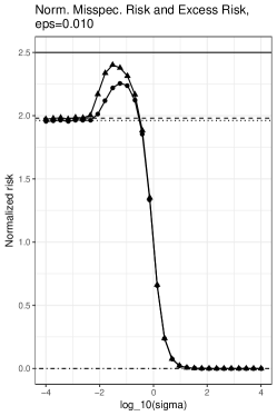
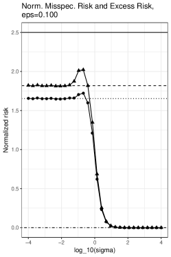
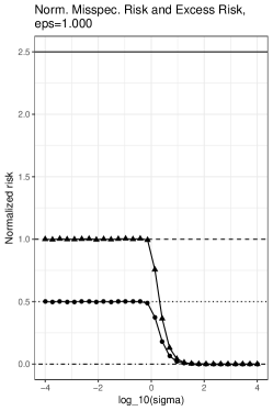
Figure 2: Empirical estimates of the normalized misspecified risk ($\bullet$) and normalized excess risk ($\blacktriangle$) plotted against $\log_{10}(\sigma)$, for the ball ${\mathcal{C}}=\{\theta\in{\mathbb{R}}^{n}:\|\theta\|\leq 1\}$ in the case $n=3$ with $\theta^{*}=(1+\epsilon,0,0)$ and $\epsilon\in\{0.01,0.1,1\}$. The solid horizontal line represents the upper bound $\delta(T_{\mathcal{C}}(\Pi_{\mathcal{C}}(\theta^{*})))=n-\frac{1}{2}=2.5$ guaranteed by (11). The dotted lines and dashed lines are the predicted low $\sigma$ limits $\frac{n-1}{(1+\epsilon)^{2}}$ and $\frac{n-1}{1+\epsilon}$ respectively. The dash-dot line is the high $\sigma$ limit $0$.

5.2 High noise limit

Although not interesting in its own right, the high noise limit of the normalized risks can help characterize the maximum risk as we discuss in the following section. Proofs for this section appear in Appendix D.

For a closed convex set ${\mathcal{C}}$ we define the core cone

$$K_{\mathcal{C}}\coloneqq\bigcap_{\theta\in{\mathcal{C}}}T_{\mathcal{C}}(\theta).$$ (72)

Recall the notation for the re-centered set $F_{\mathcal{C}}(\theta_{0})=\{\theta-\theta_{0}:\theta\in{\mathcal{C}}\}$ where $\theta_{0}\in{\mathcal{C}}$. For a vector $v\in{\mathbb{R}}^{n}$ we let ${\mathbb{R}}_{+}v\coloneqq\{\alpha u:\alpha\geq 0\}$. We have the following equivalent characterizations of the core cone.

Lemma 5.2 (Characterizations of the core cone).

Let ${\mathcal{C}}\subseteq{\mathbb{R}}^{n}$ be a closed convex set. For any $\theta_{0}\in{\mathcal{C}}$,

$$K_{\mathcal{C}}\overset{(i)}{=}\{v:{\mathbb{R}}_{+}v\subseteq F_{\mathcal{C}}(\theta_{0})\}\overset{(ii)}{=}\bigcap_{\sigma>0}\frac{F_{\mathcal{C}}(\theta_{0})}{\sigma}.$$ (73)

Additionally, the inclusion $K_{\mathcal{C}}\subseteq T_{\mathcal{C}}(\theta)$ holds for any $\theta\in{\mathcal{C}}$. If furthermore $F_{\mathcal{C}}(\theta_{0})$ is a cone, then the equality $K_{\mathcal{C}}=T_{\mathcal{C}}(\theta)$ holds if and only if $\theta_{0}-(\theta-\theta_{0})\in{\mathcal{C}}$; in particular, taking $\theta=\theta_{0}$ shows that $K_{\mathcal{C}}=T_{\mathcal{C}}(\theta_{0})=F_{\mathcal{C}}(\theta_{0})$.

Thus, up to a translation, the core cone can either be viewed as the result of shrinking ${\mathcal{C}}$ radially toward $\theta_{0}\in{\mathcal{C}}$, or as the largest cone centered at $\theta_{0}\in{\mathcal{C}}$ that is contained in ${\mathcal{C}}$. An interesting point is that $\theta_{0}\in{\mathcal{C}}$ can be chosen arbitrarily.

Furthermore, in case when ${\mathcal{C}}$ is a cone, the core cone $K_{\mathcal{C}}$ is this cone ${\mathcal{C}}$, and we can characterize which tangent cones are the “smallest” in the sense that they equal the intersection (72) of all tangent cones.

The following result shows that under a boundedness condition, the core cone characterizes both high $\sigma$ limits.

Proposition 5.3 (High noise limit).

Let ${\mathcal{C}}$ be a closed convex set. Let $\theta^{*}\in{\mathbb{R}}^{n}$ and $Y\coloneqq\theta^{*}+\sigma Z$ where $Z$ is a zero mean random vector with ${\mathbb{E}}\|Z\|^{2}<\infty$. If the condition

$$\sup_{x\in{\mathbb{R}}^{n}}\left(\|\Pi_{F_{\mathcal{C}}(\Pi_{\mathcal{C}}(\theta^{*}))}(x)\|^{2}-\|\Pi_{K_{\mathcal{C}}}(x)\|^{2}\right)<\infty.$$ (74)

holds, then

$$\lim_{\sigma\to\infty}\frac{1}{\sigma^{2}}M(\hat{\theta},\theta^{*})=\lim_{\sigma\to\infty}\frac{1}{\sigma^{2}}E(\hat{\theta},\theta^{*})=\delta(K_{\mathcal{C}}).$$ (75)

The main hurdle in applying 5.3 is verifying the condition (74). The following result covers two cases where it is easy to verify the condition.

Corollary 5.4 (Orthant and bounded sets).

Let $\theta^{*}\in{\mathbb{R}}^{n}$ and $Y\sim N(\theta^{*},\sigma^{2}I_{n})$.

• If ${\mathcal{C}}={\mathbb{R}}^{n}_{+}$ is the nonnegative orthant, then the high $\sigma$ limits are $\delta({\mathbb{R}}^{n}_{+})=n/2$.

• Let ${\mathcal{C}}$ be a closed convex set. $K_{\mathcal{C}}=\{0\}$ if and only if ${\mathcal{C}}$ is bounded, in which case both high $\sigma$ limits are $0$.

Figure 2 and Figure 3 illustrate the result of this corollary.

Verifying (74) for more general ${\mathcal{C}}$ is more difficult. We believe it might hold for polyhedral cones with any $\theta^{*}$, in which case 5.3 would imply that the high $\sigma$ limits are $\delta({\mathcal{C}})$. An interesting feature of the examples presented thus far is that the high $\sigma$ limits (including the veracity of (74)) do not depend on $\theta^{*}$.

Remark 5.5.

More generally, suppose ${\mathcal{C}}$ is a general cone. By applying 5.2 with $\theta_{0}=0$ and $\theta=\Pi_{\mathcal{C}}(\theta^{*})$, we observe that the core cone $K_{\mathcal{C}}$ is ${\mathcal{C}}$, and moreover ${\mathcal{C}}\subseteq T_{\mathcal{C}}(\Pi_{\mathcal{C}}(\theta^{*}))$, with equality if and only if $-\Pi_{\mathcal{C}}(\theta^{*})\in{\mathcal{C}}$. Thus, if the condition (74) holds, then 5.3 implies the high $\sigma$ limits are $\delta({\mathcal{C}})$, and moreover 5.2 implies that these limits equal Bellec’s upper bound (11), $\delta(T_{\mathcal{C}}(\Pi_{\mathcal{C}}(\theta^{*})))$, if and only if $\theta^{*}$ satisfies $-\Pi_{\mathcal{C}}(\theta^{*})\in{\mathcal{C}}$.

However, the condition (74) does not hold for all ${\mathcal{C}}$. One can verify numerically that the epigraph ${\mathcal{C}}\coloneqq\{u\in{\mathbb{R}}^{2}:u_{2}\geq u_{1}^{2}\}$, whose core cone is $K_{\mathcal{C}}=\{(0,u_{2}):u_{2}\geq 0\}$, does not satisfy (74). Simulations also show that the high $\sigma$ limits are larger than $\delta(K_{\mathcal{C}})=1/2$. In general, it is unclear exactly when the core cone does or does not characterize the high $\sigma$ limits.

5.3 Maximum normalized risk

Our low and high $\sigma$ limit results Theorem 3.1 and 5.3 provides an incomplete characterization of the maximum normalized risks (14). As mentioned already in (11), $\delta(T_{\mathcal{C}}(\Pi_{\mathcal{C}}(\theta^{*})))$ is an upper bound for both suprema.

In the well-specified case $\theta^{*}\in{\mathcal{C}}$, both suprema reduce to the usual normalized risk $\sigma^{-2}R(\hat{\theta},\theta^{*})$; moreover the upper bound becomes $\delta(T_{\mathcal{C}}(\theta^{*}))$, and is attained as $\sigma\downarrow 0$ by the result (7) of Oymak and Hassibi [7].

However, in the misspecified case we have shown in Theorem 3.1 that in general the low $\sigma$ limit does not attain the upper bound (11). Moreover, simulations show that in some cases even the suprema do not attain the upper bound; see Figure 2 and Figure 3. We see that for some cases the suprema are close to the upper bound, but for others it is much smaller.

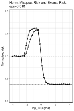
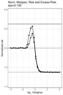
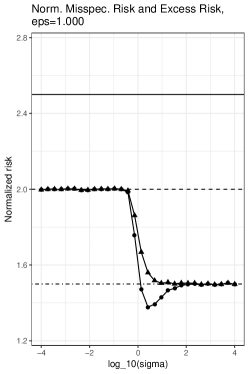
Figure 3: Empirical estimates of the normalized misspecified risk ($\bullet$) and normalized excess risk ($\blacktriangle$) plotted against $\log_{10}(\sigma)$, for the orthant ${\mathcal{C}}\coloneqq{\mathbb{R}}^{3}_{+}$ and $\theta^{*}=(1,1,-\epsilon)$ with $\epsilon\in\{0.01,0.1,1\}$. The solid horizontal line represents the upper bound $\delta(T_{{\mathcal{C}}}(\Pi_{\mathcal{C}}(\theta^{*})))=n-\frac{1}{2}$ guaranteed by (11). The dashed line is the common low $\sigma$ limit $n-1$ (see 4.1). The dash-dot line is the high $\sigma$ limit $\delta({\mathbb{R}}^{n}_{+})=3/2$.

Of course, if one can show that either the low $\sigma$ limit or the high $\sigma$ limit is equal to the upper bound $\delta(T_{\mathcal{C}}(\Pi_{\mathcal{C}}(\theta^{*})))$, then we know the upper bound is attained either as $\sigma\downarrow 0$ or $\sigma\to\infty$ respectively. However, in the settings of Theorem 3.1 and 5.3, this seldom happens. As discussed already, if ${\mathcal{C}}$ is polyhedral with nonempty interior, then the low $\sigma$ limit is strictly smaller than the upper bound. If 5.3 applies, then $K_{\mathcal{C}}=\bigcap_{\theta\in{\mathcal{C}}}T_{\mathcal{C}}(\theta)\subseteq T_{\mathcal{C}}(\Pi_{\mathcal{C}}(\theta^{*}))$ shows that the high $\sigma$ limit is typically strictly smaller than the upper bound; for the special case where ${\mathcal{C}}$ is a cone, see 5.5 for a necessary and sufficient condition for the high $\sigma$ limit to equal the upper bound.

Thus in most cases the suprema are attained at some moderate values of $\sigma$, but it is difficult to provide a characterization of these maximizing values $\sigma$, as well as the value of the suprema and whether they are close to the upper bound or not. The plots suggest that as $\theta^{*}$ gets closer to ${\mathcal{C}}$, the suprema get closer to the upper bound as well.

Appendix A Proofs of lemmas in Section 3

The next lemma is a technical device for representing the largest face of a polyhedral cone that lies in a particular hyperplane. It is useful for proving 3.3 and 3.5.

Lemma A.1 (Largest face in hyperplane).

Let ${\mathcal{K}}=\{u:Au\leq 0\}\subseteq{\mathbb{R}}^{n}$ be a polyhedral cone, where $A\in{\mathbb{R}}^{m\times n}$ has distinct rows. For each $y\in{\mathbb{R}}^{n}$, consider the subsets $J\subseteq\{1,\ldots,m\}$ satisfying

$$\{u:A_{J}u=0\}\subseteq(y-\Pi_{\mathcal{K}}(y))^{\perp}.$$ (76)

We let $J_{y}$ denote the smallest such subset.

This subset $J_{y}$ characterizes a face of ${\mathcal{K}}$ in the following way.

$${\mathcal{K}}\cap(y-\Pi_{\mathcal{K}}(y))^{\perp}=\{u:A_{J_{y}}u=0,A_{J_{y}^{c}}u\leq 0\}.$$ (77)

Proof.

The optimality condition for a projection onto a cone (22) implies $\langle y-\Pi_{\mathcal{K}}(y),u\rangle\leq 0$ for all $u\in{\mathcal{K}}$. If ${\mathcal{K}}$ contains both $u$ and $-u$, then this implies $u\in(y-\Pi_{\mathcal{K}}(y))^{\perp}$. Thus for $J=\{1,\ldots,m\}$, (76) holds because $\{u:A_{J}u=0\}\subseteq{\mathcal{K}}$. This shows the existence of subsets $J$ that satisfy (76).

Next, note that if $J$ and $J^{\prime}$ both satisfy (76), then $J\cap J^{\prime}$ does as well, because

$$\{u:A_{J\cap J^{\prime}}u=0\}=\{u+v:A_{J}u=A_{J^{\prime}}v=0\}\subseteq(y-\Pi_{\mathcal{K}}(y))^{\perp}.$$ (78)

So, letting $J_{y}$ be the intersection of all $J$ satisfying (76) yields the unique subset of minimal size.

The $\supseteq$ inclusion in (77) follows immediately from $\{u:A_{J_{y}}u=0\}\subseteq(y-\Pi_{\mathcal{K}}(y))^{\perp}$. For the other inclusion, suppose $v\in{\mathcal{K}}\cap(y-\Pi_{\mathcal{K}}(y))^{\perp}$. Then $Av\leq 0$, so it remains to verify $A_{J_{y}}v=0$. That is, if $J\subseteq\{1,\ldots,m\}$ denotes the indices $j$ for which $\langle a_{j},v\rangle=0$, we want to show $J_{y}\subseteq J$; furthermore, this reduces to showing $J$ satisfies (76), by minimality of $J_{y}$.

Any $u$ satisfying $A_{J}u=0$ can be rewritten as $u=v+w$ for some $w$ also satisfying $A_{J}w=0$. There exists some $c>0$ such that both $v+cw$ and $v-cw$ are in ${\mathcal{K}}$ because all the linear constraints outside of $J$ are strict inequalities at $v$. Then, the optimality condition for the projection onto a cone, yields $\langle v+cw,y-\Pi_{\mathcal{K}}(y)\rangle\leq 0$ and $\langle v-cw,y-\Pi_{\mathcal{K}}(y)\rangle\leq 0$. Since $v\in(y-\Pi_{\mathcal{K}}(y))^{\perp}$, this yields $w\in(y-\Pi_{\mathcal{K}}(y))^{\perp}$ and thus $u\in(y-\Pi_{\mathcal{K}}(y))^{\perp}$, which verifies that $J$ satisfies (76). ∎

Proof of 3.2.

By definition there exist an integer $m$, matrix $A\in{\mathbb{R}}^{m\times n}$, and vector $b\in{\mathbb{R}}^{m}$ such that ${\mathcal{C}}\coloneqq\{u\in{\mathbb{R}}^{n}:Au\leq b\}$. Fix $\theta^{*}\in{\mathbb{R}}^{n}$ and let $\theta_{0}\coloneqq\Pi_{\mathcal{C}}(\theta^{*})$. We will show

$$T_{\mathcal{C}}(\theta_{0})=\{u:A_{J}u\leq 0\},$$ (79)

where $J=\{j:\langle a_{j},\theta_{0}\rangle=b_{j}\}$. Then $T_{\mathcal{C}}(\theta_{0})$ is a polyhedral cone.

If $u\in T_{\mathcal{C}}(\theta_{0})$ then for some $r^{*}>0$ we have $\theta_{0}+ru\in{\mathcal{C}}$. Thus, $b_{J}\geq A_{J}(\theta_{0}+ru)=b_{J}+rA_{J}u$ which implies $A_{J}u\leq 0$.

Conversely, suppose $u$ satisfies $A_{J}u\leq 0$. Choose $r^{*}>0$ so that $r\langle a_{j},u\rangle\leq b_{j}-\langle a_{j},\theta_{0}\rangle$ for all $j\notin J$. This is possible because $b_{j}>\langle a_{j},\theta_{0}\rangle$ for each $j\notin J$. Then $\theta_{0}+r^{*}u\in{\mathcal{C}}$ so $u\in T_{\mathcal{C}}(\theta_{0})$.

Finally, we need to prove the second part of the locally polyhedral condition (LABEL:split:polyhedral_condition), which will follow if we show $T_{\mathcal{C}}(\theta_{0})\cap B_{r^{*}}(0)\subseteq F_{\mathcal{C}}(\theta_{0})$ for some $r>0$. If $u\in T_{\mathcal{C}}(\theta_{0})$ then $A_{J}u\leq 0=b_{J}-A_{J}\theta_{0}$, so it suffices to find some $r$ such that $A_{J^{c}}u\leq b_{J^{c}}-A_{J^{c}}\theta_{0}$ for any $u\in B_{r^{*}}(0)$. For each $j\notin J$, we have $\langle a_{j},\theta_{0}\rangle<b_{j}$ so there exists some $r^{*}>0$ such that all $\theta\in B_{r^{*}}(\theta_{0})$ satisfy $\langle a_{j},\theta\rangle<b_{j}$ for all $j\notin J$. Taking $u=\theta-\theta_{0}$ concludes the proof. ∎

Proof of 3.3.

Let ${\mathcal{T}}\coloneqq\{u+\Pi_{\mathcal{C}}(\theta^{*}):u\in T_{\mathcal{C}}(\Pi_{\mathcal{C}}(\theta^{*}))\}$. Using the locally polyhedral condition (LABEL:split:polyhedral_condition) and continuity [5] of $\Pi_{\mathcal{C}}$ and $\Pi_{\mathcal{T}}$, we have $\Pi_{\mathcal{T}}(\theta^{*})=\Pi_{\mathcal{C}}(\theta^{*})$ (e.g., see the verification of (37)), and thus translating yields $\Pi_{T_{\mathcal{C}}(\Pi_{\mathcal{C}}(\theta^{*}))}(\theta^{*}-\Pi_{\mathcal{C}}(\theta^{*}))=0$. Applying A.1 with $\mathcal{K}=T_{\mathcal{C}}(\Pi_{\mathcal{C}}(\theta^{*}))$, $y=\theta^{*}-\Pi_{\mathcal{C}}(\theta^{*})$, and $\Pi_{\mathcal{K}}(y)=0$ concludes the proof. ∎

Proof of 3.4.

Fix $\theta_{0}\in{\mathcal{C}}$. For any $\theta^{*}\notin{\mathcal{C}}$ such that $\Pi_{\mathcal{C}}(\theta^{*})=\theta_{0}$, 3.2 implies the locally polyhedral condition (LABEL:split:polyhedral_condition) holds, and thus 3.3 establishes that $T_{\mathcal{C}}(\Pi_{\mathcal{C}}(\theta^{*}))\cap(\theta^{*}-\Pi_{\mathcal{C}}(\theta^{*}))^{\perp}$ is a face of the tangent cone $T_{\mathcal{C}}(\theta_{0})$.

Since the tangent cone has finitely many faces, the supremum is actually a maximum over the statistical dimensions of finitely many such lower-dimensional faces. Thus it remains to show

$$\delta(T_{\mathcal{C}}(\Pi_{\mathcal{C}}(\theta^{*}))\cap(\theta^{*}-\Pi_{\mathcal{C}}(\theta^{*}))^{\perp})<\delta(T_{\mathcal{C}}(\theta_{0}))$$ (80)

for each $\theta^{*}\notin{\mathcal{C}}$ such that $\Pi_{\mathcal{C}}(\theta^{*})=\theta_{0}$.

The set $(\theta^{*}-\Pi_{\mathcal{C}}(\theta^{*}))^{\perp}$ is a hyperplane (not all of ${\mathbb{R}}^{n}$) because $\theta^{*}\notin{\mathcal{C}}$. Using the fact that the tangent cone $T_{\mathcal{C}}(\theta_{0})$ has nonempty interior (because it contains the translation $F_{\mathcal{C}}(\theta_{0})$ of ${\mathcal{C}}$), we see that the intersection $T_{\mathcal{C}}(\Pi_{\mathcal{C}}(\theta^{*}))\cap(\theta^{*}-\Pi_{\mathcal{C}}(\theta^{*}))^{\perp}$ is a face that that lies in a strictly lower-dimensional subspace of ${\mathbb{R}}^{n}$, and is therefore strictly smaller than the full cone $T_{\mathcal{C}}(\theta_{0})$. Thus, we just need to show $\delta(T^{\prime})<\delta(T)$ for any polyhedral cone $T$ with nonempty interior in ${\mathbb{R}}^{n}$, and any face $T^{\prime}$ of $T$ that lies in a strictly lower-dimensional subspace of ${\mathbb{R}}^{n}$.

For a point $x\in{\mathbb{R}}^{n}$ and a set $S\subseteq{\mathbb{R}}^{n}$ let $d(x,S)\coloneqq\inf_{\theta\in S}\|x-\theta\|$. Note that the Moreau decomposition for cones [2, Sec. B] implies $\|\Pi_{\mathcal{K}}(x)\|=d(x,{\mathcal{K}}^{\circ})$ for any $x\in{\mathbb{R}}^{n}$ and any cone ${\mathcal{K}}$, where ${\mathcal{K}}^{\circ}\coloneqq\{u\in{\mathbb{R}}^{n}:\langle u,\theta\rangle\leq 0,\forall\theta\in{\mathcal{K}}\}$ denotes the polar cone of ${\mathcal{K}}$. Since $T^{\circ}\subseteq(T^{\prime})^{\circ}$, we have

$$d(x,(T^{\prime})^{\circ})\leq d(x,T^{\circ}),\qquad\forall x\in{\mathbb{R}}^{n}.$$ (81)

Thus, if we show the random vector $Z$ has nonzero probability of being in the set

$$\mathcal{A}\coloneqq\{x\in{\mathbb{R}}^{n}:d(x,(T^{\prime})^{\circ})<d(x,T^{\circ})\}=\{x\in{\mathbb{R}}^{n}:\|\Pi_{T^{\prime}}(x)\|<\|\Pi_{T}(x)\|\},$$ (82)

then we immediately have the desired strict inequality

$$\delta(T^{\prime})={\mathbb{E}}d(Z,(T^{\prime})^{\circ})<{\mathbb{E}}d(Z,T^{\circ})=\delta(T).$$ (83)

To prove the above claim that ${\mathbb{P}}(Z\in\mathcal{A})>0$, we show below that the interior of $T$ is contained in $\mathcal{A}$; then our assumption on $Z$ will conclude the proof.

Let $x$ be in the interior of $T$. Then $x\in T\setminus T^{\prime}$. Moreover, if we let $U$ be the smallest linear subspace of ${\mathbb{R}}^{n}$ containing $T^{\prime}$, then $x\notin U$ as well. Note the the Pythagorean theorem implies

$$\|\Pi_{T}(x)\|^{2}=\|x\|^{2}=\|\Pi_{U}(x)\|^{2}+\|x-\Pi_{U}(x)\|^{2}>\|\Pi_{U}(x)\|^{2}.$$ (84)

We also have

$$\Pi_{T^{\prime}}(x)=\mathop{\rm argmin}_{\theta\in T^{\prime}}\|\theta-x\|^{2}=\mathop{\rm argmin}_{\theta\in T^{\prime}}\left\{\|\theta-\Pi_{U}(x)\|^{2}+\|\Pi_{U}(x)-x\|^{2}\right\}=\Pi_{T^{\prime}}(\Pi_{U}(x)),$$ (85)

so combining this with the above inequality (84) and the optimality condition (22) for the projection of $\Pi_{U}(x)$ onto the cone $T^{\prime}$, we have

$$\|\Pi_{T^{\prime}}(x)\|^{2}=\|\Pi_{T^{\prime}}(\Pi_{U}(x))\|^{2}=\|\Pi_{U}(x)\|^{2}-\|\Pi_{U}(x)-\Pi_{T^{\prime}}(\Pi_{U}(x))\|^{2}\leq\|\Pi_{U}(x)\|^{2}<\|\Pi_{T}(x)\|^{2},$$ (86)

and thus $x\in\mathcal{A}$. ∎

Proof of 3.5.

The lemma holds immediately if $\theta^{*}\in{\mathcal{T}}$, so we assume $\theta^{*}\notin{\mathcal{T}}$.

By translating, we may without loss of generality assume $\Pi_{\mathcal{T}}(\theta^{*})=0$ so that the cone is centered at $0$ and can be written as ${\mathcal{T}}=\{u:Au\leq 0\}$ for some number of constraints $m$ and some matrix $A\in{\mathbb{R}}^{m\times n}$. The objective then reduces to

$$\Pi_{\mathcal{T}}(y)\in(\theta^{*})^{\perp},\qquad\text{for all $y\in B_{r}(\theta^{*})$.}$$ (87)

For any $y\in{\mathbb{R}}^{n}$ let $J_{y}\subseteq\{1,\ldots,m\}$ be as defined in A.1 for our polyhedral cone ${\mathcal{T}}$; it characterizes the largest face of ${\mathcal{T}}$ that lies in $(\theta^{*})^{\perp}$. We claim there exists $r>0$ such that

$$\{u:A_{J_{y}}u=0\}\subseteq(\theta^{*})^{\perp},\quad\forall y\in B_{r}(\theta^{*}).$$ (88)

If not, then there exists a sequence of points $y_{k}\notin{\mathcal{T}}$ converging to $\theta^{*}$ such that $\{u:A_{J_{y_{k}}}u=0\}\not\subseteq(\theta^{*})^{\perp}$ for all $k$. Since there are finitely many distinct subsets $J_{y_{k}}$, we may take a subsequence and without loss of generality assume it is common subset $J=J_{y_{k}}$ for all $k$, and $\{u:A_{J}u=0\}\not\subseteq(\theta^{*})^{\perp}$. By the definition (76) of $J_{y_{k}}$, any $u$ satisfying $A_{J}u=0$ also satisfies $\langle y_{k}-\Pi_{\mathcal{T}}(y_{k}),u\rangle=0$. By continuity of $\Pi_{\mathcal{T}}$ and taking $k\to\infty$, we have $\langle\theta^{*},u\rangle=0$ as well, a contradiction.

Finally, since the optimality condition (15) for $\Pi_{\mathcal{T}}$ implies $\langle\Pi_{\mathcal{T}}(y),y-\Pi_{\mathcal{T}}(y)\rangle=0$ for any $y\in{\mathbb{R}}^{n}$, (77) implies $\Pi_{\mathcal{T}}(y)\in\{u:A_{J_{y}}u=0\}$. Combining this with (88) concludes the proof. ∎

Appendix B Proofs for Section 4.2 (isotonic regression)

B.1 Proofs of block monotone cone lemmas

Proof of 4.4.

The first claim follows from decomposing the squared Euclidean distance into blocks.

$$\min_{v\in{\mathcal{S}}_{|I_{1}|,\ldots,|I_{m}|}}\|v-z\|^{2} =\min_{x\in{\mathcal{S}}^{m}}\sum_{j=1}^{m}\sum_{i\in I_{j}}(x_{j}-z_{i})^{2}$$ (89)

$$=\min_{x\in{\mathcal{S}}^{m}}\sum_{j=1}^{m}\sum_{i\in I_{j}}((x_{j}-\bar{z}_{I_{j}})^{2}+(\bar{z}_{I_{j}}-y_{i})^{2})$$ (90)

$$=\sum_{j=1}^{m}\sum_{i\in I_{j}}(z_{i}-\bar{z}_{I_{j}})^{2}+\min_{x\in{\mathcal{S}}^{m}}\sum_{j=1}^{m}|I_{j}|(x_{j}-\bar{z}_{I_{j}})^{2}.$$ (91)

Let $Z$ and $Z^{\prime}$ be standard Gaussian in ${\mathbb{R}}^{n}$ and ${\mathbb{R}}^{m}$ respectively. If $|I_{1}|=\cdots=|I_{m}|=r$, then the first claim implies

$$\delta({\mathcal{S}}_{|I_{1}|,\ldots,|I_{m}|})\coloneqq{\mathbb{E}}\|\Pi_{{\mathcal{S}}_{|I_{1}|,\ldots,|I_{m}|}}(Z)\|^{2}\overset{(i)}{=}r{\mathbb{E}}\|\Pi_{{\mathcal{S}}^{m}}(Z^{\prime}/\sqrt{r})\|^{2}\overset{(ii)}{=}{\mathbb{E}}\|\Pi_{{\mathcal{S}}^{m}}(Z^{\prime})\|^{2}\eqqcolon\delta({\mathcal{S}}^{m})=\sum_{j=1}^{m}\frac{1}{j},$$ (92)

where (i) is due to $Z^{\prime}/\sqrt{r}\overset{d}{=}(\bar{Z}_{I_{1}},\ldots,\bar{Z}_{I_{m}})$, and (ii) is due to $\Pi_{\mathcal{C}}(cx)=c\Pi_{\mathcal{C}}(x)$ for a cone ${\mathcal{C}}$ and $c>0$ (e.g., [3, Sec. 1.6]). The statistical dimension of ${\mathcal{S}}^{m}$ is proved by Amelunxen et al. [2, Sec. D.4]. ∎

Proof of 4.5.

We use two useful properties of the statistical dimension of any cone ${\mathcal{C}}$ [2, Prop. 3.1].

• Rotational invariance: for any orthogonal transformation $Q$, we have $\delta(Q{\mathcal{C}})=\delta({\mathcal{C}})$.

• Invariance under embedding: $\delta({\mathcal{C}}\times\{0\}^{k})=\delta({\mathcal{C}})$.

Thus it suffices to provide an orthogonal transformation $Q$ such that $Q{\mathcal{S}}_{|I_{1}|,\ldots,|I_{m}|}$ is an embedding of the cone (62) into ${\mathbb{R}}^{n}$.

Let $e_{i}$ denote the $i$th standard basis vector in ${\mathbb{R}}^{n}$. Let the last element of each block be denoted $k_{j}\coloneqq\max I_{j}$ for $1\leq j\leq m$, with $k_{0}=0$ for convenience. The block monotone cone ${\mathcal{S}}_{|I_{1}|,\ldots,|I_{m}|}$ is defined by the following constraints for $u\in{\mathbb{R}}^{n}$.

$$\langle e_{i}-e_{i+1},u\rangle \leq 0, i\in\{k_{1},\ldots,k_{m}\}$$ (93a)

$$\langle e_{i}-e_{i+1},u\rangle =0, i\in\{1,\ldots,n-1\}\setminus\{k_{1},\ldots,k_{m}\}$$ (93b)

Let us focus on an arbitrary block $I_{j}$. Consider the $|I_{j}|\times|I_{j}|$ matrix

$$\tilde{A}_{j}=\begin{bmatrix}1&&\\ -1&1&\\ &-1&1\\ &&\ddots&\ddots\\ &&&-1&1\end{bmatrix}$$ (94)

Because $\tilde{A}_{j}$ is full rank, the QR decomposition implies there exists an $|I_{j}|\times|I_{j}|$ orthogonal matrix $\tilde{Q}_{j}$ such that $\tilde{R}_{j}\coloneqq\tilde{Q}_{j}\tilde{A}_{j}$ is upper triangular with positive diagonal entries, and this decomposition is unique.

The block diagonal matrix $Q$ with blocks $\tilde{Q}_{1},\ldots,\tilde{Q}_{m}$ is an $n\times n$ orthogonal matrix. Let $A$ and $R$ also be block diagonal, each constructed similarly using the $\tilde{A}_{j}$ and the $\tilde{R}_{j}$ respectively, so that $U=QA$. We consider $Q{\mathcal{S}}_{|I_{1}|,\ldots,|I_{m}|}$. We use the fact that if $v=Qu$ then $\langle b,u\rangle\leq 0\iff\langle Qb,v\rangle\leq 0$ to rewrite the constraints (93a) and (93b). The following hold for each $j=1,\ldots,m$.

• Note that the $i$th column of $A$ is $a_{i}=e_{i}-e_{i+1}$ when $k_{j-1}<i<k_{j}$. For these $i$, the equality constraints (93b) after the transformation become $0=\langle Q(e_{i}-e_{i+1}),v\rangle=\langle r_{i},v\rangle$ where $r_{i}$ is the $i$th column of $R$. Since $\tilde{R}_{j}$ is upper triangular with nonzero diagonal entries (because $\tilde{A}_{j}$ is full rank), induction on $i=k_{j-1}+1,\ldots,k_{j}-1$ implies

  $$v_{i}=0,\qquad k_{j-1}<i<k_{j}.$$ (95)

• When $j<m$, we have $e_{k_{j}}=a_{k}$ and $e_{k_{j}+1}=a_{k_{j}}+a_{k_{j}+1}+\cdots+a_{k_{j+1}}$ Thus for $j<m$ the inequality constraint $\langle e_{k_{j}}-e_{k_{j}+1},u\rangle\leq 0$ becomes

  $$0\geq\langle Q(e_{k_{j}}-e_{k_{j}+1}),v\rangle=\langle r_{k_{j}}-r_{k_{j}+1}-r_{k_{j}+2}-\cdots-r_{k_{j+1}},v\rangle=\langle r_{k_{j}}-r_{k_{j+1}},v\rangle,$$ (96)

  where the last equality is due to $\langle r_{i},v\rangle=0$ for $k_{j}<i<k_{j+1}$, by the previous point. Since $\tilde{R}_{j}$ and $\tilde{R}_{j+1}$ are each upper triangular, the inequality reduces to $r_{k_{j},k_{j}}v_{k_{j}}\leq r_{k_{j+1},k_{j+1}}v_{k_{j+1}}$, where $r_{k,k}$ denotes the $k$th diagonal entry of $R$. B.1 (proved below) computes these diagonal elements and yields

  $$\frac{v_{k_{j}}}{\sqrt{|I_{j}|}}\leq\frac{v_{k_{j+1}}}{\sqrt{|I_{j+1}|}}.$$ (97)

Therefore we have shown that $Q{\mathcal{S}}_{|I_{1}|,\ldots,|I_{m}|}$ consists of all vectors satisfying

$$\frac{v_{k_{1}}}{\sqrt{|I_{1}|}}\leq\frac{v_{k_{2}}}{\sqrt{|I_{2}|}}\leq\cdots\leq\frac{v_{k_{m}}}{\sqrt{|I_{m}|}},\text{ and }v_{i}=0,\forall i\in\{1,\ldots,n\}\setminus\{k_{1},\ldots,k_{m}\}.$$ (98)

We have thus verified the claim that $Q{\mathcal{S}}_{|I_{1}|,\ldots,|I_{m}|}$ is an embedding of (62) into ${\mathbb{R}}^{n}$.

When the blocks all have equal size $r$, the cone (62) becomes the monotone cone ${\mathcal{S}}^{m}$, whose statistical dimension is $\sum_{j=1}^{m}\frac{1}{j}$ [2, Sec. D.4]. ∎

Lemma B.1.

Consider the $n\times n$ matrix

$$A=\begin{bmatrix}1&&\\ -1&1&\\ &-1&1\\ &&\ddots&\ddots\\ &&&-1&1\end{bmatrix}.$$ (99)

There exists a unique orthogonal matrix $Q$ and a unique upper triangular matrix $R$ with positive diagonal entries such that $A=QR$. The bottom-right entry of $R$ is $r_{n,n}=1/\sqrt{n}$.

Proof.

Let $q_{i}$ be the $i$th column of $Q$. The last column $q_{n}$ is orthogonal to the span of the first $n-1$ columns of $A$, so $q_{n}$ is either $(1,\ldots,1)/\sqrt{n}$ or its negative. The positivity constraint on the diagonal entries of $R$ implies the former, and thus $r_{n,n}=\langle q_{n},e_{n}\rangle=1/\sqrt{n}$. ∎

B.2 Statistical dimension of the block monotone cone in general

In 4.5 we provided an expression for the statistical dimension of the block monotone cone ${\mathcal{S}}_{|I_{1}|,\ldots,|I_{m}|}$ when the block sizes were equal. In general, the statistical dimension can be higher or lower than $\sum_{j=1}^{m}\frac{1}{j}$. Consider the following examples for $m=3$.

4.5 implies ${\mathcal{S}}_{n-2,1,1}$ has the same statistical dimension as $\{v\in{\mathbb{R}}^{3}:v_{1}/\sqrt{n-2}\leq v_{2}\leq v_{3}\}$. As $n\to\infty$ this latter cone approaches $\{v\in{\mathbb{R}}^{3}:0\leq v_{2}\leq v_{3}\}$ which has statistical dimension $1+\left(\frac{1}{8}\cdot 2+\frac{1}{2}\cdot 1\right)=\frac{7}{4}=1.75$, which is smaller than $\sum_{j=1}^{3}\frac{1}{j}=\frac{11}{6}=1.8\bar{3}$.

On the other hand, ${\mathcal{S}}_{1,n-2,1}$ has the same statistical dimension as $\{v\in{\mathbb{R}}^{3}:v_{1}\leq v_{2}/\sqrt{n-2}\leq v_{3}\}$. As $n\to\infty$ this latter cone approaches $\{v\in{\mathbb{R}}^{3}:v_{1}\leq 0,v_{3}\geq 0\}$ which has statistical dimension $1+\frac{1}{2}+\frac{1}{2}=2$, which is larger than $1.8\bar{3}$.

We suspect that the approach used to prove the statistical dimension of ${\mathcal{S}}^{n}$ [2, Sec. D.4], which uses the theory of finite reflection groups, cannot be generalized for ${\mathcal{S}}_{|I_{1}|,\ldots,|I_{m}|}$, due to the asymmetry of (62). However, using a result of Klivans and Swartz [6], it is possible to show that the average statistical dimension among all block monotone cones with a given [unordered] set of $m$ block sizes is $H_{m}$ [1, Prop. 6.6].

B.3 Proof of 4.3

When applying Theorem 3.1, it is useful to characterize ${\mathcal{S}}^{n}$ and its tangent cones using conic generators. If $T\subseteq{\mathbb{R}}^{n}$ is a cone and there exist $x_{1},\ldots,x_{p}\in T$ such that

$$T=\left\{\sum_{i=1}^{p}\alpha_{i}x_{i}:\alpha_{i}\geq 0,\forall i\right\},$$ (100)

then we call $x_{1},\ldots,x_{p}$ the conic generators of $T$, and write

$$T=\operatorname{cone}\{x_{1},\ldots,x_{p}\}.$$ (101)

Lemma B.2.

Let $\theta^{*}\in{\mathbb{R}}^{n}$ and let ${\mathcal{C}}\subseteq{\mathbb{R}}^{n}$ be closed and convex. If the tangent cone $T_{\mathcal{C}}(\Pi_{\mathcal{C}}(\theta^{*}))$ is generated by $x_{1},\ldots,x_{p}\in{\mathbb{R}}^{n}$, i.e. $T_{\mathcal{C}}(\Pi_{\mathcal{C}}(\theta^{*}))=\operatorname{cone}\{x_{1},\ldots,x_{p}\}$, then

$$T_{\mathcal{C}}(\Pi_{\mathcal{C}}(\theta^{*}))\cap(\theta^{*}-\Pi_{\mathcal{C}}(\theta^{*}))^{\perp}=\operatorname{cone}(\{x_{1},\ldots,x_{p}\}\cap(\theta^{*}-\Pi_{\mathcal{C}}(\theta^{*}))^{\perp}).$$ (102)

Proof of B.2.

The inclusion $\supset$ is immediate, so it remains to prove the inclusion $\subseteq$. Note that the optimality condition (15) implies $\langle\theta^{*}-\Pi_{\mathcal{C}}(\theta^{*}),x\rangle\leq 0$ for any $x\in T_{\mathcal{C}}(\Pi_{\mathcal{C}}(\theta^{*}))$. In particular, if $v\in T_{\mathcal{C}}(\Pi_{\mathcal{C}}(\theta^{*}))\cap(\theta^{*}-\Pi_{\mathcal{C}}(\theta^{*}))^{\perp}$, then $v$ can be written as the conical combination $v=\sum_{i=1}^{p}\alpha_{i}x_{i}$ with $\alpha_{i}\geq 0$, and we have

$$0=\langle\theta^{*}-\Pi_{\mathcal{C}}(\theta^{*}),v\rangle=\sum_{i=1}^{p}\alpha_{i}\underbrace{\langle\theta^{*}-\Pi_{\mathcal{C}}(\theta^{*}),x_{i}\rangle}_{\leq 0}.$$ (103)

Thus, if a generator $x_{i}$ is not in the hyperplane $(\theta^{*}-\Pi_{\mathcal{C}}(\theta^{*}))^{\perp}$, then $\alpha_{i}=0$, so $x_{i}$ does not contribute in the conical combination of $v$. Thus, $v$ can be written as a conical combination of generators in $(\theta^{*}-\Pi_{\mathcal{C}}(\theta^{*}))^{\perp}$. ∎

We are now ready to prove 4.3.

Proof of 4.3.

By Theorem 3.1, it suffices to prove that the statistical dimension term is $\sum_{k=1}^{K}\delta\left({\mathcal{S}}_{|I_{1}^{k}|,\ldots,|I^{k}_{m_{k}}|}\right)$.

For $p\geq 1$ let

$$M_{p}\coloneqq\begin{bmatrix}-1&-1&\cdots&-1\\ 1&1&\cdots&1\\ &1&\cdots&1\\ &&\ddots&\vdots\\ &&&1\end{bmatrix}\in{\mathbb{R}}^{(p+1)\times p}.$$ (104)

The rows of $M_{p}$ are the conic generators of ${\mathcal{S}}^{p}$.

Suppose first that $\Pi_{{\mathcal{S}}^{n}}(\theta^{*})$ is constant, so that $K=1$ and $J_{1}=\{1,\ldots,n\}$. Then $\Pi_{{\mathcal{S}}^{n}}(\theta^{*})=(\mu_{1},\mu_{1},\ldots,\mu_{1})$ where $\mu_{1}\coloneqq\frac{1}{n}\sum_{i=1}^{n}\theta^{*}_{i}$; this follows directly by minimizing $\sum_{i=1}^{n}(\theta_{i}^{*}-\mu_{1})^{2}$ with respect to $\mu_{1}$.

The finest partition $(I^{1}_{1},\ldots,I^{1}_{m_{1}})$ of $J_{1}$ into blocks satisfying (58) can be constructed greedily as follows. Begin populating $I^{1}_{1}$ with the elements of $\{1,\ldots,n\}$ in order, stopping as soon as the mean of the elements of $I^{1}_{1}$ is $\mu_{1}$. Then begin populating $I^{1}_{2}$ with the remaining elements in order, again stopping when the mean of the elements in $I^{1}_{2}$ is $\mu_{1}$. Continue in this manner until the last element $n$ is placed in a subset $I^{1}_{m_{1}}$. The mean of the elements of this last subset $I^{1}_{m_{1}}$ is $\mu_{1}$ as well, since the mean of all components of $\theta^{*}$ is $\mu_{1}$. Thus this partition satisfies (58). To establish uniqueness, note that if some other partition of $J_{1}$ satisfies (58), then our partition $(I^{1}_{1},\ldots,I^{1}_{m_{1}})$ must be a refinement, due to the greedy construction.

Because $\Pi_{{\mathcal{S}}^{n}}(\theta^{*})$ is constant, the tangent cone there is $T_{{\mathcal{S}}^{n}}(\Pi_{{\mathcal{S}}^{n}}(\theta^{*}))={\mathcal{S}}^{n}$ [3, Prop. 3.1], which is generated by the rows of $M_{n}$. In order to use B.2, we need to determine which rows of $M_{n}$ are in the hyperplane $(\theta^{*}-\Pi_{{\mathcal{S}}^{n}}(\theta^{*}))^{\perp}$. We already know the mean of the components of $\theta^{*}-\Pi_{{\mathcal{S}}^{n}}(\theta^{*})$ is zero, so the first two rows are in the hyperplane.

We claim that exactly $m_{1}-1$ of the remaining $n-1$ rows of $M_{n}$ also lie in the hyperplane. Explicitly, if $(I^{1}_{1},\ldots,I^{1}_{m_{1}})$ is without loss of generality assumed to be sorted in increasing order, then the remaining rows of $M_{n}$ that lie in the hyperplane are the indicator vectors for

$$\bigcup_{j=u}^{m_{k}}I^{1}_{j},\qquad 2\leq u\leq m_{k}.$$ (105)

No other rows of $M_{n}$ can be in the hyperplane, else there would exist a finer partition of $J_{1}$.

So, B.2 implies $T_{{\mathcal{S}}^{n}}(\Pi_{{\mathcal{S}}^{n}}(\theta^{*}))\cap(\theta^{*}-\Pi_{{\mathcal{S}}^{n}}(\theta^{*}))^{\perp}$ is the cone generated by $(-1,\ldots,-1)$, $(1,\ldots,1)$, and the indicator vectors of the subsets (105), otherwise known as the cone of nondecreasing vectors that are piecewise constant on the blocks $I^{1}_{1},\ldots,I^{1}_{m_{1}}$. Its statistical dimension is denoted by $\delta({\mathcal{S}}_{|I^{1}_{1}|,\ldots,|I^{1}_{m_{1}}|})$. This concludes the proof in the case when $\Pi_{{\mathcal{S}}^{n}}(\theta^{*})$ is constant.

We now turn to the general case where $\Pi_{{\mathcal{S}}^{n}}(\theta^{*})$ is piecewise constant with values $\mu_{1}<\cdots<\mu_{K}$ on $J_{1},\ldots,J_{K}$ respectively. We claim

$$\mu_{k}=\frac{1}{|J_{k}|}\sum_{i\in J_{k}}\theta^{*}_{i}.$$ (106)

Since ${\mathcal{S}}^{n}$ is a cone, the projection satisfies $\langle\theta^{*}-\Pi_{{\mathcal{S}}^{n}}(\theta^{*}),x\rangle\leq 0$ for all $x\in{\mathcal{S}}^{n}$, with equality if $x=\Pi_{\mathcal{C}}(\theta^{*})$ (e.g., [3, Sec. 1.6]). Letting $x_{1},\ldots,x_{n+1}$ be the conic generators of ${\mathcal{S}}^{n}$ (the rows of $M_{n}$), we have $\Pi_{\mathcal{C}}(\theta^{*})=\sum_{i=1}^{n+1}\alpha_{i}x_{i}$ for some coefficients $\alpha_{i}\geq 0$. Then,

$$0=\langle\theta^{*}-\Pi_{{\mathcal{S}}^{n}}(\theta^{*}),\Pi_{\mathcal{C}}(\theta^{*})\rangle=\sum_{i=1}^{n+1}\alpha_{i}\underbrace{\langle\theta^{*}-\Pi_{{\mathcal{S}}^{n}}(\theta^{*}),x_{i}\rangle}_{\leq 0},$$ (107)

which implies $\langle\theta^{*}-\Pi_{{\mathcal{S}}^{n}}(\theta^{*}),x_{i}\rangle=0$ if $\alpha_{i}>0$. Consequently, if $\Pi_{{\mathcal{S}}^{n}}(\theta^{*})$ changes value from component $j-1$ to $j$, then $\sum_{i=j}^{n}[\theta^{*}_{i}-(\Pi_{{\mathcal{S}}^{n}}(\theta^{*}))_{i}]=0$. Thus (106) holds.

By Proposition 3.1 of [3], the tangent cone is

$$T_{{\mathcal{S}}^{n}}(\Pi_{{\mathcal{S}}^{n}}(\theta^{*}))={\mathcal{S}}^{n_{1}}\times\cdots\times{\mathcal{S}}^{n_{K}},$$ (108)

which is generated by the rows of the block diagonal matrix

$$A\coloneqq\begin{bmatrix}M_{n_{1}}\\ &\ddots\\ &&M_{n_{K}}\end{bmatrix}.$$ (109)

To find which rows of $A$ are in the hyperplane $(\theta^{*}-\Pi_{{\mathcal{S}}^{n}}(\theta^{*}))^{\perp}$, we can treat each block $M_{n_{k}}$ separately and repeat the above argument. Doing so shows that $T_{{\mathcal{S}}^{n}}(\Pi_{{\mathcal{S}}^{n}}(\theta^{*}))\cap(\theta^{*}-\Pi_{{\mathcal{S}}^{n}}(\theta^{*}))^{\perp}$ is the cone of vectors that are piecewise constant on $(I^{1}_{1},\ldots,I^{1}_{m_{1}},\ldots,I^{K}_{1},\ldots,I^{K}_{m_{K}})$ and are increasing within each of the blocks $(J_{1},\ldots,J_{K})$. The statistical dimension of this cone is $\sum_{k=1}^{K}\delta({\mathcal{S}}_{|I^{k}_{1}|,\ldots,|I^{k}_{m_{k}}|})$. ∎

Appendix C Proof of 5.1

Let $r\coloneqq\|\theta^{*}\|$. By rotating the problem, we may without loss of generality assume $\theta^{*}=(r,0,\ldots,0)$.

Let $E\coloneqq\{Y\in B_{(r-1)/2}(\theta^{*})\}$. Then we have $E\subseteq\{Y\notin{\mathcal{C}}\}$, so under the event $E$ we have $\hat{\theta}(Y)=Y/\|Y\|$. Noting $\|Y\|^{2}=\|\theta^{*}+\sigma Z\|^{2}=r^{2}+2\sigma rZ_{1}+\sigma^{2}\|Z\|^{2}$, we have

$$\frac{1}{\sigma^{2}}\|\hat{\theta}(Y)-\Pi_{\mathcal{C}}(\theta^{*})\|^{2}=\frac{1}{\sigma^{2}}\left(\frac{r+\sigma Z_{1}}{\sqrt{r^{2}+2\sigma rZ_{1}+\sigma^{2}\|Z\|^{2}}}-1\right)^{2}+\frac{\sum_{i=2}^{n}Z_{i}^{2}}{r^{2}+2\sigma rZ_{1}+\sigma^{2}\|Z\|^{2}}.$$ (110)

The second term converges to $r^{-2}\sum_{i=2}^{n}Z_{i}^{2}$ as $\sigma\downarrow 0$. We show the first term vanishes as $\sigma\downarrow 0$. Defining $g(\sigma)\coloneqq\|\theta^{*}+\sigma Z\|$, we have

$$g(\sigma) =\sqrt{r^{2}+2\sigma rZ_{1}+\sigma^{2}\|Z\|^{2}}$$ (111)

$$g^{\prime}(\sigma) =\frac{rZ_{1}+\sigma\|Z\|^{2}}{g(\sigma)}$$ (112)

$$g^{\prime\prime}(\sigma) =\frac{\|Z\|^{2}}{g(\sigma)}-\frac{(rZ_{1}+\sigma\|Z\|^{2})g^{\prime}(\sigma)}{g(\sigma)^{2}}$$ (113)

Moreover we have $g(0)=r$, $g^{\prime}(0)=Z_{1}$, and $g^{\prime\prime}(0)=(\|Z\|^{2}-Z_{1}^{2})/r$. Then by L’Hôpital’s rule,

$$\lim_{\sigma\downarrow 0}\frac{1}{\sigma}\left(\frac{r+\sigma Z_{1}}{\sqrt{r^{2}+2\sigma rZ_{1}+\sigma^{2}\|Z\|^{2}}}-1\right)$$ (114)

$$=\lim_{\sigma\downarrow 0}\frac{r+\sigma Z_{1}-g(\sigma)}{\sigma g(\sigma)}=\lim_{\sigma\downarrow 0}\frac{Z_{1}-g^{\prime}(\sigma)}{g(\sigma)+\sigma g^{\prime}(\sigma)}=\frac{Z_{1}-Z_{1}}{r+0}=0.$$ (115)

Note $\boldsymbol{\mathbf{1}}_{E}\to 1$ almost surely as $\sigma\downarrow 0$. Thus, $\sigma^{-2}\|\hat{\theta}(Y)-\Pi_{\mathcal{C}}(\theta^{*})\|^{2}\boldsymbol{\mathbf{1}}_{E}\to r^{-2}\sum_{i=2}^{n}Z_{i}^{2}$ almost surely. By the upper bound (11) we may use the dominated convergence theorem to get

$$\lim_{\sigma\downarrow 0}\frac{1}{\sigma^{2}}{\mathbb{E}}_{\theta^{*}}\left[\|\hat{\theta}(Y)-\Pi_{\mathcal{C}}(\theta^{*})\|^{2}\boldsymbol{\mathbf{1}}_{E}\right]=\frac{1}{r^{2}}\sum_{i=2}^{n}{\mathbb{E}}Z_{i}^{2}=\frac{n-1}{r^{2}}.$$ (116)

To conclude the proof of the first limit (70a), note that

$$\lim_{\sigma\downarrow 0}\frac{1}{\sigma^{2}}{\mathbb{E}}_{\theta^{*}}\left[\|\hat{\theta}(Y)-\Pi_{\mathcal{C}}(\theta^{*})\|^{2}\boldsymbol{\mathbf{1}}_{E^{c}}\right]=0,$$ (117)

which holds by the argument used in the proof of Theorem 3.1 (e.g., see the second term in (29)).

A similar proof holds for the second limit (70b). Let $E$ and $g(\sigma)$ be the same as before. Then

$$\frac{1}{\sigma^{2}}\left(\|\hat{\theta}(Y)-\theta^{*}\|^{2}-\|\Pi_{\mathcal{C}}(\theta^{*})-\theta^{*}\|^{2}\right)$$ (118)

$$=\frac{1}{\sigma^{2}}\left(\frac{r+\sigma Z_{1}}{\sqrt{r^{2}+2\sigma rZ_{1}+\sigma^{2}\|Z\|^{2}}}-r\right)^{2}+\frac{\sum_{i=2}^{n}Z_{i}^{2}}{r^{2}+2\sigma rZ_{1}+\sigma^{2}\|Z\|^{2}}-\frac{(r-1)^{2}}{\sigma^{2}}$$ (119)

$$=\frac{1}{\sigma^{2}}\left[\left(\frac{r+\sigma Z_{1}}{g(\sigma)}-r\right)^{2}-(r-1)^{2}\right]+\frac{\sum_{i=2}^{n}Z_{i}^{2}}{r^{2}+2\sigma rZ_{1}+\sigma^{2}\|Z\|^{2}}.$$ (120)

Again, the second term tends to $r^{-2}\sum_{i=2}^{n}Z_{i}^{2}$ as $\sigma\downarrow 0$. To handle the first term we use L’Hôpital’s rule again. Let

$$h(\sigma) \coloneqq\frac{r+\sigma Z_{1}}{g(\sigma)}-r$$ (121)

$$h^{\prime}(\sigma) =\frac{Z_{1}}{g(\sigma)}-\frac{(r+\sigma Z_{1})g^{\prime}(\sigma)}{g(\sigma)^{2}}$$ (122)

$$h^{\prime\prime}(\sigma) =-\frac{Z_{1}g^{\prime}(\sigma)}{g(\sigma)^{2}}+2\frac{(r+\sigma Z_{1})g^{\prime}(\sigma)^{2}}{g(\sigma)^{3}}-\frac{Z_{1}g^{\prime}(\sigma)+(r+\sigma Z_{1})g^{\prime\prime}(\sigma)}{g(\sigma)^{2}}$$ (123)

Recalling the limits $g(0)=r$, $g^{\prime}(0)=Z_{1}$, and $g^{\prime\prime}(0)=(\|Z\|^{2}-Z_{1}^{2})/r$, we have $h(\sigma)\to-(r-1)$, $h^{\prime}(\sigma)\to 0$, and

$$h^{\prime\prime}(0)=-\frac{Z_{1}^{2}}{r^{2}}+2\frac{rZ_{1}^{2}}{r^{3}}-\frac{Z_{1}^{2}+\|Z\|^{2}-Z_{1}^{2}}{r^{2}}=\frac{Z_{1}^{2}-\|Z\|^{2}}{r^{2}}.$$ (124)

Then, L’Hôpital’s rule allows us to compute the limit of the first term.

$$\lim_{\sigma\downarrow 0}\frac{1}{\sigma^{2}}\left[\left(\frac{r+\sigma Z_{1}}{g(\sigma)}-r\right)^{2}-(r-1)^{2}\right]$$ (125)

$$=\lim_{\sigma\downarrow 0}\frac{h(\sigma)^{2}-(r-1)^{2}}{\sigma^{2}}=\lim_{\sigma\downarrow 0}\frac{h(\sigma)h^{\prime}(\sigma)}{\sigma}=\lim_{\sigma\downarrow 0}(h^{\prime}(\sigma)^{2}+h(\sigma)h^{\prime\prime}(\sigma))=\frac{(r-1)(\|Z\|^{2}-Z_{1}^{2})}{r^{2}}.$$ (126)

Combining terms yields

$$\frac{1}{\sigma^{2}}\left(\|\hat{\theta}(Y)-\theta^{*}\|^{2}-\|\Pi_{\mathcal{C}}(\theta^{*})-\theta^{*}\|^{2}\right)\boldsymbol{\mathbf{1}}_{E}\to\frac{(r-1)(\|Z\|^{2}-Z_{1}^{2})+\sum_{i=2}^{n}Z_{i}^{2}}{r^{2}}=\frac{\sum_{i=2}^{n}Z_{i}^{2}}{r},$$ (127)

so again by dominated convergence with the upper bound (11), we have

$$\frac{1}{\sigma^{2}}{\mathbb{E}}_{\theta^{*}}\left[\left(\|\hat{\theta}(Y)-\theta^{*}\|^{2}-\|\Pi_{\mathcal{C}}(\theta^{*})-\theta^{*}\|^{2}\right)\boldsymbol{\mathbf{1}}_{E}\right]\to\frac{n-1}{r}.$$ (128)

To conclude the proof of (70b), note that

$$\frac{1}{\sigma^{2}}{\mathbb{E}}_{\theta^{*}}\left[\left(\|\hat{\theta}(Y)-\theta^{*}\|^{2}-\|\Pi_{\mathcal{C}}(\theta^{*})-\theta^{*}\|^{2}\right)\boldsymbol{\mathbf{1}}_{E^{c}}\right]\to 0,$$ (129)

which was proved in the proof of Theorem 3.1 (see (46)).

Appendix D Proofs for Section 5.2

The following lemma shows that the left-hand side of (74) is nonnegative.

Lemma D.1.

For any $\theta_{0}\in{\mathcal{C}}$,

$$\|\Pi_{F_{\mathcal{C}}(\theta_{0})}(x)\|^{2}\geq\|\Pi_{K_{\mathcal{C}}}(x)\|^{2}.$$ (130)

Proof of D.1.

Because $K_{\mathcal{C}}$ is a cone, we have $\langle x,\Pi_{K_{\mathcal{C}}}(x)\rangle=\|\Pi_{K_{\mathcal{C}}}(x)\|^{2}$. Since $K_{\mathcal{C}}\subseteq F_{\mathcal{C}}(\theta_{0})$, the optimality condition for $\Pi_{F_{\mathcal{C}}(\theta_{0})}(x)$ implies $\langle x-\Pi_{F_{\mathcal{C}}(\theta_{0})}(x),\Pi_{K_{\mathcal{C}}}(x)\rangle\leq 0$ and thus

$$\|\Pi_{K_{\mathcal{C}}}(x)\|^{2}\leq\langle\Pi_{F_{\mathcal{C}}(\theta_{0})}(x),\Pi_{K_{\mathcal{C}}}(x)\rangle\leq\|\Pi_{F_{\mathcal{C}}(\theta_{0})}(x)\|\|\Pi_{K_{\mathcal{C}}}(x)\|.$$ (131)

Thus $\|\Pi_{F_{\mathcal{C}}(\theta_{0})}(x)\|\geq\|\Pi_{K_{\mathcal{C}}}(x)\|$ and $M_{\theta_{0}}\geq 0$. ∎

Proof of 5.2.

We first prove the equalities (i) and (ii).

1. Let $v\in\{u:{\mathbb{R}}_{+}u\subseteq F_{\mathcal{C}}(\theta_{0})\}$ and let $\theta\in{\mathcal{C}}$. For any $c>0$ we have $\theta_{0}+cv\in{\mathcal{C}}$, and convexity implies $\theta+\alpha(\theta_{0}+cv-\theta)\in{\mathcal{C}}$ for all $\alpha\in[0,1]$. For large $c$ we have $\|\theta_{0}+cv-\theta\|>1$ and thus $\theta+\frac{\theta_{0}+cv-\theta}{\|\theta_{0}+cv-\theta\|}\in{\mathcal{C}}$. Taking $c\to\infty$ and using the fact that ${\mathcal{C}}$ is closed yields $\theta+\frac{v}{\|v\|}\in{\mathcal{C}}$ and thus $v\in T_{\mathcal{C}}(\theta)$. Since $\theta$ was arbitrary, we have $v\in K_{\mathcal{C}}$.

   Conversely, suppose $v\in K_{\mathcal{C}}$. Let $c^{*}\coloneqq\sup\{c>0:\theta_{0}+cv\in{\mathcal{C}}\}$. The supremum is over a nonempty set because $v\in T_{\mathcal{C}}(\theta_{0})$. Suppose for sake of contradiction that $c^{*}<\infty$. Since ${\mathcal{C}}$ is closed, $\theta_{0}+c^{*}v\in{\mathcal{C}}$. Thus $v\in T_{\mathcal{C}}(\theta_{0}+c^{*}v)$ which implies $\theta_{0}+(c^{*}+\alpha)v\in{\mathcal{C}}$ for some $\alpha>0$, contradicting the definition of $c^{*}$. Thus $c^{*}=\infty$ and $\theta_{0}+cv\in{\mathcal{C}}$ for all $c>0$.

2. Both sides can be expressed as the set of $v\in{\mathbb{R}}^{n}$ satisfying $\theta_{0}+\sigma v\in{\mathcal{C}}$ for all $\sigma>0$.

We now prove the second part of the lemma. The definition (72) implies $K_{\mathcal{C}}\subseteq T_{\mathcal{C}}(\theta)$ for any $\theta\in{\mathcal{C}}$.

Now, assume $F_{\mathcal{C}}(\theta_{0})$ is a cone. If the reverse inclusion $T_{\mathcal{C}}(\theta)\subseteq F_{\mathcal{C}}(\theta)$ holds, then $\theta_{0}-\theta\in T_{\mathcal{C}}(\theta)=F_{\mathcal{C}}(\theta)$ so $\theta_{0}-(\theta-\theta_{0})\in{\mathcal{C}}$. Conversely, suppose $\theta_{0}-(\theta-\theta_{0})\in{\mathcal{C}}$. If $v\in T_{\mathcal{C}}(\theta)$, then $\theta+cv\in{\mathcal{C}}$ for some $c>0$. By convexity, $\theta_{0}+cv/2\in{\mathcal{C}}$, so $v\in F_{\mathcal{C}}(\theta_{0})$. Thus $T_{\mathcal{C}}(\theta)\subseteq F_{\mathcal{C}}(\theta)$. ∎

Proof of 5.3.

We use $Y$ instead of $\theta^{*}+\sigma Z$ throughout the proof, but note that $Y$ depends on $\sigma$.

Without loss of generality we can translate the problem so that $\Pi_{\mathcal{C}}(\theta^{*})=0$.

In view of (21), we may use the dominated convergence theorem on $\sigma^{-2}\|\Pi_{\mathcal{C}}(Y)-\Pi_{\mathcal{C}}(\theta^{*})\|^{2}$, so

$$\lim_{\sigma\to\infty}\frac{1}{\sigma^{2}}{\mathbb{E}}\|\Pi_{\mathcal{C}}(Y)-\Pi_{\mathcal{C}}(\theta^{*})\|^{2}$$ (132)

$$={\mathbb{E}}\lim_{\sigma\to\infty}\frac{1}{\sigma^{2}}\|\Pi_{\mathcal{C}}(Y)-\Pi_{\mathcal{C}}(\theta^{*})\|^{2} {\mathbb{E}}\|Z\|^{2}$$ dom. conv. with (133)

$$={\mathbb{E}}\lim_{\sigma\to\infty}\frac{1}{\sigma^{2}}\|\Pi_{\mathcal{C}}(Y)\|^{2}$$ (134)

$$\overset{(i)}{=}{\mathbb{E}}\|\Pi_{K_{\mathcal{C}}}(Z)\|^{2}=\delta(K_{\mathcal{C}}),$$ (135)

where we verify the equality (i) below.

Similarly, (21) allows us to use the dominated convergence theorem again for the excess risk.

$$\lim_{\sigma\to\infty}\frac{1}{\sigma^{2}}\left({\mathbb{E}}\|\Pi_{\mathcal{C}}(Y)-\theta^{*}\|^{2}-\|\Pi_{\mathcal{C}}(\theta^{*})-\theta^{*}\|^{2}\right)$$ (136)

$$={\mathbb{E}}\lim_{\sigma\to\infty}\frac{1}{\sigma^{2}}\left(\|\Pi_{\mathcal{C}}(Y)-\theta^{*}\|^{2}-\|\theta^{*}\|\right) {\mathbb{E}}\|Z\|^{2}$$ dom. conv. with (137)

$$={\mathbb{E}}\lim_{\sigma\to\infty}\frac{1}{\sigma^{2}}\left(\|\Pi_{\mathcal{C}}(Y)\|^{2}-2\langle\Pi_{\mathcal{C}}(Y),\theta^{*}\rangle\right)$$ (138)

$$\overset{(ii)}{=}{\mathbb{E}}\|\Pi_{K_{\mathcal{C}}}(Z)\|^{2}=\delta(K_{\mathcal{C}}).$$ (139)

It remains to verify (i) and (ii).

1. $$\phantom{{}\leq{}}\left|\frac{1}{\sigma^{2}}\|\Pi_{\mathcal{C}}(Y)\|^{2}-\|\Pi_{K_{\mathcal{C}}}(Z)\|^{2}\right|$$ (140)

   $$\leq\frac{1}{\sigma^{2}}\left|\|\Pi_{\mathcal{C}}(Y)\|^{2}-\|\Pi_{K_{\mathcal{C}}}(Y)\|^{2}\right|+\left|\frac{1}{\sigma^{2}}\|\Pi_{K_{\mathcal{C}}}(Y)\|^{2}-\|\Pi_{K_{\mathcal{C}}}(Z)\|^{2}\right|$$ (141)

   $$\leq\frac{c}{\sigma^{2}}+\left|\|\Pi_{K_{\mathcal{C}}}(\theta^{*}/\sigma+Z)\|^{2}-\|\Pi_{K_{\mathcal{C}}}(Z)\|^{2}\right| K_{\mathcal{C}}$$ D.1; is a cone (142)

   $$\overset{\sigma\to\infty}{\longrightarrow}0. x\mapsto\|\Pi_{K_{\mathcal{C}}}(x)\|^{2}$$ is continuous (143)

2. We already showed $\|\Pi_{\mathcal{C}}(Y)\|^{2}/\sigma^{2}\to\|\Pi_{K_{\mathcal{C}}}(Z)\|^{2}$, so it suffices to show the cross term vanishes. Indeed, we have $\|\Pi_{\mathcal{C}}(Y)\|/\sigma\to\|\Pi_{K_{\mathcal{C}}}(Z)\|$, so

   $$\frac{1}{\sigma^{2}}\left|\langle\Pi_{\mathcal{C}}(Y),\theta^{*}\rangle\right|\leq\frac{1}{\sigma^{2}}\|\Pi_{\mathcal{C}}(Y)\|\|\theta^{*}\|\overset{\sigma\to\infty}{\longrightarrow}0.$$ (144)

∎

Proof of 5.4.

We begin with the first claim. Since ${\mathcal{C}}={\mathbb{R}}^{n}_{+}$ is a cone, we have $K_{\mathcal{C}}={\mathbb{R}}^{n}_{+}$. Provided we verify (74), the result follows from 5.3. Let $\theta\coloneqq\Pi_{\mathcal{C}}(\theta^{*})$ and fix $x\in{\mathbb{R}}^{n}$. Then some casework yields

$$\|\Pi_{F_{\mathcal{C}}(\theta)}(x)\|^{2}-\|\Pi_{K_{\mathcal{C}}}(x)\|^{2}=\sum_{i=1}^{n}\max\{x_{i},-\theta_{i}\}^{2}-\sum_{i=1}^{n}\max\{x_{i},0\}^{2}\leq\sum_{i=1}^{n}\theta_{i}^{2}=\|\theta\|^{2}\eqqcolon c.$$ (145)

We now turn to the second claim. If ${\mathcal{C}}$ is bounded, then by 5.2, $K_{\mathcal{C}}=\{u:{\mathbb{R}}_{+}u\subseteq F_{\mathcal{C}}(\theta_{0})\}=\{0\}$ for any $\theta_{0}\in{\mathcal{C}}$.

Conversely, suppose ${\mathcal{C}}$ is unbounded and fix $\theta_{0}\in{\mathcal{C}}$. Let

$$U_{r}\coloneqq\{v\in S^{n-1}:\theta_{0}+cv\notin{\mathcal{C}}\text{ for some }c\in(0,r)\}.$$ (146)

This set is open: if $(v_{n})$ is a sequence in $U_{r}^{c}$ converging to $v$, then the fact that ${\mathcal{C}}$ is closed implies $\theta_{0}+rv_{n}\in{\mathcal{C}}$ for all $n$, and consequently $\theta_{0}+rv\in{\mathcal{C}}$ and finally $v\in U^{c}_{r}$.

If $\bigcup_{r>0}U_{r}$ is an open cover of the compact set $S^{n-1}$, then $S^{n-1}\subseteq U_{r}$ for some $r>0$, which implies ${\mathcal{C}}\subseteq B_{r}(\theta_{0})$, a contradiction. Thus, some direction $v\in S^{n-1}$ does not lie in $\bigcup_{r>0}U_{r}$, i.e., $\theta_{0}+cv\in{\mathcal{C}}$ for all $c\geq 0$. This implies $cv\in K_{\mathcal{C}}$ for all $c\geq 0$.

We now apply 5.3. If ${\mathcal{C}}$ is bounded, then so is $F_{\mathcal{C}}(\Pi_{\mathcal{C}}(\theta^{*}))$. Choosing $c$ large enough so that $F_{\mathcal{C}}(\Pi_{\mathcal{C}}(\theta^{*}))$ lies in the ball of radius $c$ suffices to satisfy (74). Then 5.3 implies that the high $\sigma$ limits are $\delta(K_{\mathcal{C}})=0$. ∎

References

- Amelunxen and Lotz [2015] Amelunxen, D. and M. Lotz (2015). Intrinsic volumes of polyhedral cones: a combinatorial perspective. arXiv preprint arXiv:1512.06033.
- Amelunxen et al. [2014] Amelunxen, D., M. Lotz, M. B. McCoy, and J. A. Tropp (2014). Living on the edge: Phase transitions in convex programs with random data. Information and Inference, iau005.
- Bellec [2015] Bellec, P. C. (2015). Sharp oracle inequalities for least squares estimators in shape restricted regression. arXiv preprint arXiv:1510.08029.
- Groeneboom and Jongbloed [2014] Groeneboom, P. and G. Jongbloed (2014). Nonparametric Estimation under Shape Constraints: Estimators, Algorithms and Asymptotics, Volume 38. Cambridge University Press.
- Hiriart-Urruty and Lemaréchal [2012] Hiriart-Urruty, J.-B. and C. Lemaréchal (2012). Fundamentals of convex analysis. Springer Science & Business Media.
- Klivans and Swartz [2011] Klivans, C. J. and E. Swartz (2011). Projection volumes of hyperplane arrangements. Discrete & Computational Geometry 46(3), 417.
- Oymak and Hassibi [2013] Oymak, S. and B. Hassibi (2013). Sharp mse bounds for proximal denoising. Foundations of Computational Mathematics, 1–65.
- Pal [2008] Pal, J. K. (2008). Spiking problem in monotone regression: Penalized residual sum of squares. Statistics & Probability Letters 78(12), 1548–1556.
- Robertson et al. [1988] Robertson, T., F. T. Wright, and R. L. Dykstra (1988). Order restricted statistical inference. Wiley Series in Probability and Mathematical Statistics: Probability and Mathematical Statistics. Chichester: John Wiley & Sons Ltd.
- Tibshirani [1996] Tibshirani, R. (1996). Regression shrinkage and selection via the lasso. Journal of the Royal Statistical Society. Series B (Methodological), 267–288.
- Wu et al. [2015] Wu, J., M. C. Meyer, and J. D. Opsomer (2015). Penalized isotonic regression. Journal of Statistical Planning and Inference 161, 12–24.
- Zhang [2002] Zhang, C.-H. (2002). Risk bounds in isotonic regression. Ann. Statist. 30(2), 528–555.