Towards an Analytic Construction of the Wavefunction of Boson Stars

Abstract

Light scalar fields can form gravitationally bound compact objects called boson stars. The profile of boson stars in the Newtonian limit is described by the Gross-Pitaevskii-Poisson equations. We present a semi-analytic solution to these equations and construct the profile of boson stars formed by a non-interacting scalar field. Our solution is stable with respect to numerical errors and has accuracy better than $10^{-6}$ over the entire range.

I Introduction

Axions are an attractive solution 1977PhRvL..38.1440P ; 1977PhRvD..16.1791P ; 1978PhRvL..40..223W ; 1978PhRvL..40..279W ; 1981PhLB..104..199D to the strong CP problem of QCD 1976PhLB…63..334C ; 1976PhRvL..37..172J , and also provide an attractive and natural dark matter candidate (for reviews see Kim:2008hd ; Cheng:1987gp ). This has motivated multiple search strategies for axions and axion-like particles 1983PhRvL..51.1415S ; 1985PhRvD..32.2988S ; 2010PhRvL.104d1301A ; 2011PhRvD..84l1302H ; Rybka:2014cya ; Sikivie:2013laa ; 2012PhRvD..85c5018B ; Horns:2012jf ; Budker:2013hfa ; Graham:2013gfa ; 1999NIMPA.425..480Z ; Stadnik:2013raa . It has also been argued that ultra-light axions Hui:2016ltb can solve problems encountered by the usual CDM models 2011AJ….141..193O ; 1993MNRAS.264..201K ; 1999ApJ…522…82K ; 2000PhRvL..84.4525K .

For all these purposes, it is important to understand the spatial structure of axion-like particles if they constitute dark matter. Most importantly, it is crucial to know whether or not these particles clump into compact objects (see Liebling:2012fv for a review). The Jeans instability 1985MNRAS.215..575K ; Bianchi:1990mha ; 1994PhRvL..72.2516S ; Mielke:2000mh ; 1986PhRvL..57.2485C indicates that a uniform density of axions is unstable, indicating the formation of large compact objects (sometimes called boson stars 1968PhRv..172.1331K ; Ruffini:1969qy ). The boson stars are prevented from completely collapsing by a bosonic analogue of the Fermi pressure in white dwarfs 1926MNRAS..87..114F .

Once the boson stars form, further cosmological evolution can occur by scattering of these boson stars off other boson stars, as well as baryonic matter Eby:2017xaw . Such scatterings may either enhance or decrease the number of these objects. To analyze these scatterings, we must have a detailed understanding of the bound states, including their energies and profiles.

At least for fairly dilute systems, the compact objects are bound states of a nonlinear Gross-Pitaevskii-Poisson equations, which we re-derive below. Numerical solutions to these equation have found the bound state energies and mass-radius relation, both in the cases with no self-interactions, as well as including self interactions, either attractive or repulsive Ruffini:1969qy ; Barranco:2010ib ; 2007JCAP…06..025B ; 1989PhRvA..39.4207M ; 1996PhRvD..53.2236L ; 2000NewA….5..103G ; 2003PhRvD..68b3511A ; Chavanis:2011zm ; Eby:2014fya ; Eby:2015hsq ; Yang:2015paa ; Kan:2017uhj . However, the profiles are only available numerically; they are computationally expensive to find and are difficult to extend to perturbations of the boson stars. Furthermore, they tend to have numerical instabilities in the tails of the profile. The author of Chavanis:2011zi follows a different approach: using a simple Gaussian ansatz for the density profile they were able to obtain the mass-radius relation and ground-state energy within a 10% deviation of the numerical solution. The Gross-Pitaevskii-Poisson equations have also been studied in the context of quantum state reduction by Penrose1998 ; Moroz:1998dh ; Tod1992 .

In this paper, we introduce a combination of analytical and numerical methods to find approximate solutions to the Gross-Pitaevskii-Poisson equations. We illustrate this for the case of no self-interactions among the bosons (the interacting case will be treated in an upcoming paper Kling:2017hjm ). We also perform a detailed analysis of the accuracy of our results. We show that our method is much less computationally expensive than previous approaches, nevertheless we demonstrate that we find excellent agreement with a full numerical solution over the entire parameter range. Furthermore, our method is numerically stable and does not diverge far away from the star, which can occur for a purely numerical approach.

II The Gross-Pitaevskii-Poisson Equations

II.1 Derivation

Let us consider a complex scalar field $\phi(\vec{r},t)$ described by the Lagrangian

$$\mathcal{L}=g^{\mu\nu}(\partial_{\mu}\phi^{*})(\partial_{\nu}\phi)-m^{2}(\phi^{*}\phi)-\frac{\lambda}{2}(\phi^{*}\phi)^{2}$$ (1)

We can then expand the field $\phi$ in spherical harmonics

$$\phi(\vec{r},t)=\sum_{nlm}R_{nl}(r)Y_{lm}(\theta,\phi)e^{-iE_{nlm}t}.$$ (2)

We assume that only the ground state $(n,l,m)=(1,0,0)$ is populated. In this case the field takes the simple form $\phi(\vec{r},t)=(2E/N)^{-\frac{1}{2}}\psi(r)e^{-iEt}$, where we denote the ground-state energy as $E$. The real function $\psi(r)$ describes the radial profile of the star and is sometimes called the wavefunction. We have chosen a normalization $\int\psi^{2}dV=1$, which allows us to identify $\psi^{2}$ with the probability density. Let us further make two simplifying assumptions

Newtonian Gravity

The field is only weakly coupled to gravity such that we can use a Newtonian approximation. This allows us to introduce the Newtonian potential $\Phi$ in the metric $g_{\mu\nu}=\text{diag}(1+2\Phi,-1,-1,-1)$. The Newtonian potential is related to the energy density via the Poisson equation $\nabla^{2}\Phi=4\pi G\rho$.

Non-Relativistic

The ground state is non-relativistic. In this case we can write $E=m+e$ with binding energy $e\ll m$. This implies $e\psi,\Phi\psi,\nabla\psi\ll m\psi$.

The equation of motion is the Klein-Gordon equation, $\Box\phi+m^{2}\phi+\lambda|\phi|^{2}\phi=0$, which we can write in terms of the wavefunction as

$$(1+2\Phi)^{-1}\partial_{t}^{2}\psi-\nabla^{2}\psi+m^{2}\psi+\frac{N\lambda}{2m}\psi^{3}=0.$$ (3)

In the non-relativistic approximation we can write

$$e\psi=-\frac{1}{2m}\nabla^{2}\psi+m\Phi\psi+\frac{N\lambda}{4m^{2}}\psi^{3}$$ (4)

and recover the Schrödinger-type equation. For our non-relativistic approximation to be consistent, the last term should be sufficiently small i.e. $\frac{N\lambda}{4m^{2}}\psi^{2}\ll m$.

The energy density of the complex scalar field is

$$\rho=|\partial_{t}\phi|^{2}+|\nabla\phi|^{2}+m^{2}|\phi|^{2}+\lambda|\phi|^{4}\approx Nm\psi^{2}$$ (5)

where we used the non-relativistic approximation in the last step. Newtons equation therefore takes the simple form

$$\nabla^{2}\Phi=4\pi GNm\psi^{2}$$ (6)

II.2 Scaling Symmetry of the Gross-Pitaevskii-Poisson System

As derived above, the ground state of the self-gravitating boson star in the non-relativistic limit can be described by a wavefunction $\psi(r)$ and a gravitational potential $\Phi(r)$ satisfying the Gross-Pitaevskii-Poisson equations given in (4) and (6). For the remainder of this paper, we will focus on the non-interacting case $\lambda=0$, and postpone the discussion of finite self-interactions $\lambda\neq 0$ to a separate study Kling:2017hjm . For simplification, let us introduce the following dimensionless variables,

$$x=2rm,\;\;V=\frac{e}{2m}-\frac{\Phi}{2},\;\;\text{and}\;\;S=\sqrt{\frac{\pi GN}{2m}}\psi$$ (7)

The equations (4) and (6) become

$$\nabla^{2}V=-S^{2}\quad\text{and}\quad\nabla^{2}S=-VS.$$ (8)

The wavefunction normalization condition $\int\psi^{2}dV=1$ can be rewritten as

$$\int_{0}^{\infty}x^{2}S^{2}dx=GMm,$$ (9)

where we introduced the star mass $M=Nm$. These equations describe the hydrostatic equilibrium of the boson star, in which the gravitational attraction caused by the potential $V$ is balanced by a repulsive quantum pressure. This quantum pressure arises from Heisenberg’s uncertainty principle and prevents the system from gravitational collapse.

Let us note that Eq. 8 and 9 are invariant under the scaling

$$x\to\frac{x}{f},\quad S\to f^{2}S,\quad V\to f^{2}V,\quad M\to fM.$$ (10)

where $f$ is a scaling factor. This implies that solutions corresponding to different masses $M$ can be related to a unique solution by rescaling. To obtain the unique solution, we have to fix the scale by choosing a reference scale $k$. Although there are many different ways to fix $k$, a particularly useful choice for our discussion is to set $-k^{2}=V(\infty)=\frac{e}{2m}$ which transforms as $k\to fk$. We can then introduce the scale invariant coordinate $z$, wavefunction $s$, potential $v$ and mass $\beta$ via

$$z=kx,\;\;S=k^{2}s,\;\;V=k^{2}v,\;\;GMm=2k\beta.$$ (11)

Note that $S$ and $V$ are functions of the scaling dependent coordinate $x$ while $s$ and $v$ are functions of the scale independent coordinate $z$. Using the scale independent variables, we can write the Gross-Pitaevskii-Poisson equations as

$$\nabla^{2}s=-sv\;\;\;\text{and}\;\;\nabla^{2}v=-s^{2}\;\;\;\text{with}\;\;v(\infty)=-1.$$ (12)

To obtain the solution corresponding to a boson star with mass $M$, we then have to perform the rescaling given in Eq. 11 with $k=\frac{GMm}{2\beta}$. In the following section, we will obtain an approximate analytical form for $s,v$ and the mass parameter $\beta$.

III Series Expansions

It has been shown Tod1992 ; Choquard:2007aa that the Gross-Pitaevskii-Poisson system given by (12) has a unique square normalizable solution for $s,v$ with $s>0$ for all values of $z$. The authors of Moroz:1998dh also provide a numerical solution. However, the authors have also shown that this numerical solution will diverge at some finite value of $z$ and can therefore not be used to describe the profile at large radius. The author of Chavanis:2011zi follows a different approach and approximates the density profile by a Gaussian, which is able to approximately reproduce thermodynamical properties of the boson star but otherwise fails to describe the profile, in particular at large radius. We attempt to solve this problem by providing an analytical expression for $s$ and $v$ which describes the profile at all radii with high precision.

III.1 Expansion at Small Radius: $z=0$

Since both $s$ and $v$ are well behaved around $z=0$, we can expand them in a series expansion

$$s=\sum_{n=0}^{\infty}s_{n}z^{n}\;\;\text{and}\;\;v=\sum_{n=0}^{\infty}v_{n}z^{n}\ .$$ (13)

We can then write the Laplacian on the left hand side of Eq. 12 as

$$\nabla s=s^{\prime\prime}+\frac{2}{z}s^{\prime}=\sum_{n=0}^{\infty}(n+2)(n+3)\;s_{n+2}\;z^{n}.$$ (14)

and the right hand side as a Cauchy product

$$sv=\Bigg{[}\sum_{i=0}^{\infty}s_{i}z^{i}\Bigg{]}\Bigg{[}\sum_{j=0}^{\infty}v_{j}z^{j}\Bigg{]}=\sum_{n=0}^{\infty}\sum_{m=0}^{n}s_{m}v_{n-m}z^{n}.$$ (15)

By matching the coefficients in Eq. 12 we obtain the recursion relations

$$(n+2)(n+3)s_{n+2} =-\sum_{m=0}^{n}s_{m}v_{n-m},$$ (16)

$$(n+2)(n+3)v_{n+2} =-\sum_{m=0}^{n}s_{m}s_{n-m}.$$

Note that requiring the profile to be smooth at the origin implies $s_{1}=v_{1}=0$ and therefore also all odd coefficients $s_{2n+1},v_{2n+1}$ vanish. The profile at small radius $z$ can therefore be fully parametrized in terms of the wavefunction and potential at the origin: $s_{0}$ and $v_{0}$. We can obtain $s_{0}$ and $v_{0}$ from a fit to the numerical solution, as discussed in appendix A.

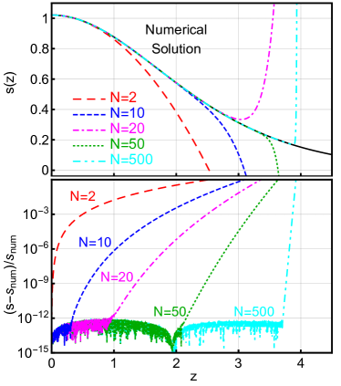
Figure 1: The upper panel shows the numerical solution (solid black) and truncated series expansion (colored dashed lines) of the central wavefunction. The lower panel shows the accuracy $(s_{(N)}-s_{num})/s_{num}$ of the truncated series expansion with respect to the numerical solution.

For practical purposes, we will truncate the infinite series of Eq. 13 at some $N$. This is shown in Fig. 1. The upper panel shows both the numerical solution as well as the truncated expansion $s_{(N)}$ for different values of $N$. The lower panel shows the deviations of the truncated expansion from the numerical solution. We can see that already a small number of terms in the series expansion provides a sub-percent level accuracy for the inner part of the profile. A better accuracy can be obtained by including more terms in the expansion. However, the accuracy of the series expansion is limited by the accuracy of $s_{0}$ and $v_{0}$ which in Fig. 1 is about $10^{-12}$. Note that the series expansion of Eq. 13 diverges at $z>4$ and a different parametrization has to be chosen.

III.2 Expansion at Large Radius: $z=\infty$

At large radius $z\to\infty$, we expect the wavefunction to decrease at least exponentially, $\psi\sim e^{-kr}$, and the potential to approach the Newtonian potential of a central point mass $\Phi\approx\frac{GM}{r}$. A series expansion at large radius must be able to reproduce these limits. Let us choose the following general ansatz for the form of the solution

$$s=\sum_{n,m=0,0}^{\infty,\infty}s^{n}_{m}\left(\frac{e^{-z}}{z^{\sigma}}\right)^{n}z^{-m},\;\;\;v=\sum_{n,m=0,0}^{\infty,\infty}v^{n}_{m}\left(\frac{e^{-z}}{z^{\sigma}}\right)^{n}z^{-m}$$ (17)

Here we assume the existence of a $\sigma\in\mathbb{R}$, whose meaning will become clear later. The Laplacian of $s$ can be written as

$$\nabla^{2}s=\sum_{n,m=0,0}^{\infty,\infty}\Big{(}s^{n}_{m}n^{2}+2s^{n}_{m-1}n(n\sigma+m-2)$$ (18)

$$+s^{n}_{m-2}(n\sigma+m-3)(n\sigma+m-2)\Big{)}\left(\frac{e^{-z}}{z^{\sigma}}\right)^{n}z^{-m}$$

Note that we introduced the short-hand notation $s_{n,-1}=s_{n,-2}=0$. The right hand side of Eq. 12 can be rewritten as Cauchy product:

$$sv =\left[\sum_{i,a=0,0}^{\infty,\infty}s^{i}_{a}\left(\frac{e^{-z}}{z^{\sigma}}\right)^{i}z^{-a}\right]\left[\sum_{j,b=0,0}^{\infty,\infty}v^{j}_{b}\left(\frac{e^{-z}}{z^{\sigma}}\right)^{j}z^{-b}\right]$$ (19)

$$=\sum_{n,m=0,0}^{\infty,\infty}\left(\sum_{p,q=0,0}^{n,m}s^{p}_{q}\;v^{n-p}_{m-q}\right)\left(\frac{e^{-z}}{z^{\sigma}}\right)^{n}z^{-m}$$

By matching the coefficients, Eq. 12 we obtain the recursion relations

$$\sum_{p,q=0,0}^{n,m} s^{p}_{q}v^{n-p}_{m-q}+n^{2}\,s^{n}_{m}+2n(n\sigma+m-2)\;s^{n}_{m-1}$$ (20)

$$+(n\sigma+m-2)(n\sigma+m-3)s^{n}_{m-2}=0$$

$$\sum_{p,q=0,0}^{n,m} s^{p}_{q}s^{n-p}_{m-q}+n^{2}\,v^{n}_{m}+2n(n\sigma+m-2)\;v^{n}_{m-1}$$ (21)

$$+(n\sigma+m-2)(n\sigma+m-3)v^{n}_{m-2}=0.$$

Let us note the following properties of $s$ and $v$: i) Normalizability requires $s^{0}_{0}=0$. Eq. 20 then implies that all coefficients $s^{0}_{m}$ vanish as well. This means that the wavefunction decays at least exponentially. ii) Eq. 21 then implies that all $v^{0}_{m}=0$ for $m>1$. This means that at large radius, the potential is described by the Newtonian potential $v^{(0)}=v^{0}_{0}+\frac{v^{0}_{1}}{z}$. All other terms in the expansion of $v$ are at least exponentially suppressed. iii) Eq. 20 and 21 further imply that the potential contains only non-vanishing components $v^{n}_{m}$ for even $n$ while the wavefunction only has non-vanishing components $s^{n}_{m}$ for odd $n$.

IV The Solution for the Wavefunction

IV.1 The Wavefunction at Leading Order

Using Eq. 20 and 21, we are able to recursively calculate all coefficients in the expansion of $s$ and $v$. Let us first analyze the $n=1$ expansion of $s$ which provides us both a leading order approximation and a deeper understanding about the form of the solution. We have seen before that at leading order the potential is given by $v^{(0)}=v^{0}_{0}+\frac{v^{0}_{1}}{z}$. Setting $m=0$, Eq. 20 reads $s^{1}_{0}=-s^{1}_{0}v^{0}_{0}$ which implies $v^{0}_{0}=-1$ as expected from our scale choice which fixes $v(\infty)=-1$. Setting $m=1$, Eq. 20 reads

$$s^{1}_{1}+2(\sigma-1)s^{1}_{0}=-s^{1}_{1}v^{0}_{0}-s^{1}_{0}v^{0}_{1}$$ (22)

which implies $v^{0}_{1}=2(1-\sigma)$. This is a remarkable result: the exponent $\sigma$ in the series expansion is related to the the total mass of the system. In the notation of Eq. 11, we can write $\sigma=1-\frac{1}{2}v^{0}_{1}=1-\beta$. Let us now calculate the remaining coefficients by setting $m=M+1$ with $M\geq 1$. Then Eq. 20 can be written as

$$s^{1}_{M+1} v^{0}_{0}+s^{1}_{M}v^{0}_{1}+s^{1}_{M+1}+2(\sigma+M-1)s^{1}_{M}$$ (23)

$$+(\sigma+M-1)(\sigma+M-2)s^{1}_{M-1}=0$$

We can therefore recursively compute the coefficients $s^{1}_{M}$ by

$$s^{1}_{M}=-\frac{(\sigma+M-1)(\sigma+M-2)}{2M}s^{1}_{M-1}.$$ (24)

Using the rising factorials $(x)_{n}=x(x+1)(x+2)\cdots(x+n-1)$, $(x)_{0}=1$ we can write the coefficients explicitly as

$$s^{1}_{M}=s^{1}_{0}\frac{(\sigma)_{M}(\sigma-1)_{M}}{M!}\cdot(-2)^{-M}$$ (25)

The leading order wavefunction $s^{(1)}$ can therefore be written as

$$s^{(1)}=\alpha\;\frac{e^{-z}}{z^{1-\beta}}\sum_{m=0}^{\infty}\left(\frac{(1-\beta)_{m}(-\beta)_{m}}{m!}\;(-2z)^{-m}\right)$$ (26)

Here we have introduced the normalization parameter $\alpha=s^{1}_{0}$. The far-field solution is described by only two free parameters: the wavefunction normalization $\alpha$ and the total mass parameter $\beta$. At very large radius, the wavefunction approaches $s=\alpha e^{-z}z^{\beta-1}$.

Let us note that we can rewrite the far-field solution as

$$s^{(1)}=\frac{\alpha}{2^{\beta}z}W_{\beta,-\frac{1}{2}}(2z)=\frac{\alpha}{2^{\beta}z}e^{-z}U(-\beta,0,2z)$$ (27)

where $W_{\beta,-\frac{1}{2}}(2z)$ is the Whittaker function which can also be expressed in terms of the confluent hypergeometric function $U$. This result is not surprising: when considering the leading order potential $v^{(0)}=-1+\frac{2\beta}{z}$, Eq. 12 turns into the Whittaker equations. For a more detailed discussion on different representations of the leading order wavefunction, see appendix B.

It is known that the series expansion of the confluent hypergeometric function $U(a,b,z)$, and therefore also the expansion of $s^{(1)}$, are not Cauchy convergent. However, the infinite sum has a finite value and behaves convergently for a finite number of terms. This is illustrated in the upper panel of Fig. 2 where we show the coefficients $s^{1}_{m}$. We can see that they converge for $m<6$ while they start to diverge again for $m>6$. Let us therefore split the function $s^{(1)}$ into a finite series $s^{(1)}_{(M)}$ truncated after $M$ terms and the corresponding remainder $R_{M}$:

$$s^{(1)}=s^{(1)}_{(M)}+R^{1}_{M}\;\;\text{with}\;\;s^{(1)}_{(M)}=\sum_{m=0}^{M}s^{1}_{m}\frac{e^{-z}}{z^{\beta-1}}z^{-m}$$ (28)

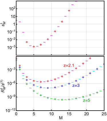
Figure 2: Coefficients $s^{1}_{m}$ of the leading order series expansion of $s^{(1)}$ as given in Eq. 25 (upper panel) and remainder $R^{1}_{M}$ as defined in Eq. 28 for different values of $z$. In both panels, positive values are indicated by a ‘$+$’ while negative values are indicated by a ‘$-$’.

In the right panel of Fig. 2 we show the relative size of the remainder $R^{1}_{M}$ with respect to $s^{(1)}$ for different values of $z$. We can see that finite series first converges quickly, even for values of $z$ close the convergence radius $z>2$. At some $M$, which depends on the value of $z$, the remainder reaches a minimum and diverges for large $M$. Note that the coefficients $s^{1}_{m}$ and therefore also the remainders $R_{M}$ are oscillating which allows the infinite series $s^{(1)}$ to be finite. In this work, we will avoid the problem of divergence by truncating the series expansion of $s^{(1)}$ at $m=M$ and ignoring the remainder. This precision of this approximation should be sufficient for most applications.

Let us now compare the leading order approximation with the numerical solution. To obtain the expansion parameters $\alpha$ and $\beta$, we perform a fit of the leading order expansion to the numerical solution, as explained in appendix A. In the upper panel of Fig. 3 we compare the full leading order approximation $s^{(1)}$ and the truncated series $s^{(1)}_{(M)}$ for different $M$ to the numerical solution. We can see that the full leading order series expansion $s^{(1)}$ converges to the numerical profile for $z>2$ and is already well described by the truncated series with $M=1$.

The lower panel shows the normalized differences between the truncated series expansion and the full leading order solution, $(s^{(1)}_{(M)}-s^{(1)})/s^{(1)}$, and deviation of the full leading order solution compared to the numerical solution. For increasing $z$, the differences between the numerical solution and the leading order solution $s^{(1)}$ become exponentially small. For $z\gtrsim 12$ we can see that the precision of the leading order approximation $s^{(1)}$ starts to be limited by the precision of the expansion parameters $\alpha$ and $\beta$, which we estimated to be of the order $10^{-9}$. The colored dashed lines show the remainder $R^{1}_{M}$ of the truncated series expansion $s^{(1)}_{(M)}$. We can see the for $M=4$ the uncertainty due to truncation is comparable to the uncertainty of the input parameters.

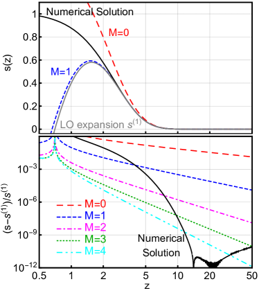
Figure 3: The upper panel shows the numerical solution (solid black line), the truncated leading order series expansion $s^{(1)}_{(M)}$ (colored dashed lines) and the full leading order series expansion $s^{(1)}$ (solid gray line) of the wavefunction. The lower panel shows the accuracy $(s^{(1)}_{(M)}-s^{(1)})/s^{(1)}$ of the truncated leading order series expansion with respect to the full leading order series expansion, as indicated by the colored dashed lines. The solid black line in the lower panel shows the accuracy of the leading order series expansion with respect to the numerical solution: $(s_{num}-s^{(1)})/s^{(1)}$.

At small $z$, we can see that difference between the numerical solution an $s^{(1)}$ increase and higher order terms $N>1$ start to be important.

IV.2 Next to Leading Order Contributions

In the previous section we have analyzed the leading order $N=1$ contribution of the series expansion in Eq. 20 to the wavefunction. We found that at large $z\gtrsim 12$, the contribution from next-to-leading order terms $N>1$ is smaller than the uncertainty induced by the uncertainty of the parameter $\alpha$ and $\beta$. We concluded that in this range the $N>1$ terms can be safely ignored. However, at intermediate $z$ in the range $2<z<12$, the next to leading order terms become important, as we have seen in Fig. 3 and terms of higher order in $N$ have to be included. Let us introduce the truncated solution $s^{(N)}_{(M)}$ and the corresponding remainder $R^{N}_{M}$ via

$$s=s^{(N)}_{(M)}+R^{N}_{M}\;\;\text{with}\;\;s^{(N)}_{(M)}=\sum_{n,m=0,0}^{N,M}s^{n}_{m}\left(\frac{e^{-z}}{z^{\beta-1}}\right)^{n}z^{-m}$$ (29)

In the upper panel of Fig. 4 we show the truncated expansion $s^{(N)}_{(M)}$ for the wavefunction for different choices of $N$, fixing $M=4$. The lower panel shows the corresponding deviations of the truncated expansion from the numerical solution. We can see that the series always diverges for $z<1$. Including the $N=3$ and $N=5$ terms will increase the accuracy of our series expansion for an intermediate radius $z\approx 3$ to an $\mathcal{O}(10^{-5})$ level. Taking into account additional terms $N>5$ does not significantly increase the accuracy of the expansion. In this case, the dominant contribution to the remainder comes from neglected terms with $m>M$, which become more important at small $z$.

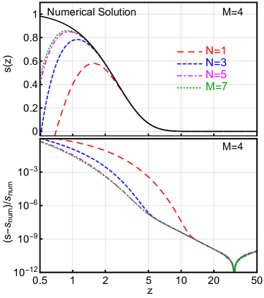
Figure 4: The upper panel shows the numerical solution (solid black) and truncated series expansion $s^{(N)}_{(M)}$ of the wavefunction. The lower panel shows the accuracy $(s^{(N)}_{(M)}-s_{num})/s_{num}$ of the truncated series expansion with respect to the numerical solution. We fix $M=4$.

IV.3 Combined Result and Matching

We can now combine the two truncated solutions, $s_{(N)}$ and $s^{(N)}_{(M)}$, obtained for both small and large values of $z$ by matching them at a matching point $z^{*}$. This is shown for $s_{(N)}$ with $N=10$ and $s^{(N)}_{(M)}$ with $N=1$, $M=1$ in the upper panel of Fig. 5. Here the truncated solution takes the simple form

$$s=\begin{cases}1.021-0.159z^{2}+1.63\cdot 10^{-2}z^{4}&\hbox{\multirowsetup$\text{ for }z<2.5$}\\ \;\,-1.42\cdot 10^{-3}z^{6}+1.14\cdot 10^{-4}z^{8}&\\ \;\,-8.74\cdot 10^{-6}z^{10}&\\ &\\ e^{-z}\cdot z^{0.7526}\left(3.4951-\frac{2.3053}{z}\right)&\text{ for }z>2.5\\ \end{cases}$$ (30)

We can see that already such few terms in the series expansion are sufficient to describe the wavefunction well. The accuracy is at the few percent level at the matching point $z=2.5$ and orders of magnitude better at small and large $z$, as shown in the lower panel. A precision of $10^{-5}$ at the matching point can be achieved using $s_{(N)}$ with $N=50$ and $s^{(N)}_{(M)}$ with $N=5$, $M=4$, where the precision at small and large $z$ is again limited by the precision of the expansion parameters $s_{0}$, $v_{0}$, $\alpha$ and $\beta$ at the $10^{-12}$ level.

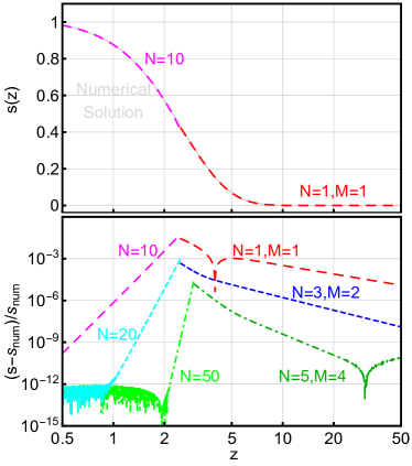
Figure 5: The upper panel shows the truncated series expansion of the wavefunction $s_{10}$ at small radius (magenta curve) and $s^{1}_{1}$ at large radius (red curve), matched at an intermediate value of $z$. The solid gray line shows the numerical solution. The lower panel shows the accuracy of the truncated series expansion with respect to the numerical solution for different truncations $N,M$.

We can also determine the expansion parameters by matching the small and large radius wavefunction and their derivatives at a matching point $z^{*}$. We have performed such a matching using $s_{(N)}$ with $N=250$ and $s^{(N)}_{(M)}$ with $N=10$ and $M=6$ and obtain

$$s_{0}=1.0215035\pm 4.46\cdot 10^{-6}$$ (31)

$$v_{0}=0.9383304\pm 2.67\cdot 10^{-6}$$

$$\alpha=3.4951958\pm 3.17\cdot 10^{-5}$$

$$\beta=1.7526505\pm 6.34\cdot 10^{-6}$$

To estimate the uncertainty associated with the matching procedure, we performed multiple matchings for $3<z^{*}<3.5$. The obtained values for expansion parameters are consistent with those in Eq. 32 obtained through the fitting of the large radius solution but have a significantly worse precision. This is not surprising, since the precision of our series expansion is expected to be worst at the matching point $z^{*}$.

V Conclusion

We have found a semi-analytic solution to the coupled Poisson-Newton equations describing dilute boson stars. We have shown that our solution is stable to numerical errors, and that it reproduces the numerical results with accuracy better than $10^{-5}$ over the entire range. Improvements in accuracy can easily be attained for a small expense of numerical work.

There are many possible applications of our methods. The simplest one is to consider interacting bosons, when a potential for the bosons is added. Such a potential can significantly modify the solution, because the interactions can be much stronger than gravitational. Rotation can also modify the solution. In all these case, the large number of parameters makes it impractical to find purely numerical solutions; our semi-analytical method would be better suited for these problems.

Another open question is the stability of these solutions. For example, it is not known how the boson stars are affected by external perturbations e.g. by another star nearby. Once again, an accurate knowledge of the profiles is a requirement for the stability analysis. We hope to return to these and other questions in future work.

Appendix A Numerical Integration and Fitting

To obtain a numerical solution, it is convenient to use the variables $S$, $V$ and coordinate $x$ given in Eq. 11 with a reference scale $k$ chosen such that $V(0)=1$. As shown in Tod1992 , the solutions of Eq. 8 can then be parametrized by the central value of the wavefunction, $S_{0}=S(0)$ and categorized into three distinct classes: for $S_{0}>S_{0}^{*}$ the wavefunction diverges for at large radius towards positive infinity, for $S_{0}=S_{0}^{*}$ the wavefunction converges to zero, is positive definite and square integrable, while for $S_{0}<S_{0}^{*}$ the wavefunction diverges for at large radius towards negative infinity.

Using a Runge-Kutta 4 method with constant step size $\Delta_{x}$, we perform the numerical integration until the wavefunction starts to diverge and iteratively optimize the central value of the wavefunction $S_{0}$ to find $S_{0}^{*}$. The precision of the wavefunction needed for the numerical solution to stay finite until a large value of $x$, which is needed to fit the large range solution, increases exponentially with the radial coordinate $x$. In this study we use a precision of 35 significant figures for $S_{0}$, providing a converging numerical solution for $x<35$. The accuracy of the numerical solution is limited by the step size $\Delta_{x}$. In this study, we use $\Delta_{x}=10^{-3}$, providing an accuracy of the solution of order $\mathcal{O}\left(\Delta_{x}^{4}\right)\approx 10^{-12}$.

To obtain the expansion parameters $\alpha,\beta$, we fit the Newtonian potential $V(x)=-k^{2}+\frac{2k\beta}{x}$ and the Whittaker solution $S(x)=\frac{k\alpha}{2^{\beta}x}W_{\beta,-\frac{1}{2}}(2kx)$ to the numerical solution for $V$ and $S$ at large $x$. To avoid systematic effects due to the truncation of subleading terms $n>1$ of the series expansion in Eq. 17, we restrict the fitting range to $x>x^{*}$, where the fraction of mass outside radius $x^{*}$ contributed less than $10^{-12}$ to the total mass of the boson star. The expansion parameters at small radius can then be obtained through $s_{0}=k^{-2}S_{0}$ and $v_{0}=k^{-2}$. We find that

$$s_{0} =1.02149303631\pm 1.4\cdot 10^{-10}$$ (32)

$$v_{0} =0.93832284019\pm 1.3\cdot 10^{-10}$$

$$\alpha =3.4951309897\phantom{9}\pm 5.1\cdot 10^{-9}$$

$$\beta =1.7526648513\phantom{9}\pm 1.3\cdot 10^{-9}$$

The uncertainty of $s_{0},v_{0}$ and $\beta$ were estimated by the difference of the best fit values to potential and wavefunction. For $\alpha$ we state the uncertainty of wavefunction fit.

Appendix B Representations of the Leading Order Wavefunction

When considering only the potential $v^{(0)}=-1+\frac{2\beta}{z}$, Eq. 12 can be written as

$$\frac{d^{2}}{dz^{2}}(2zs^{(1)})+2zs^{(1)}\left(-1+\frac{2\beta}{z}\right)=0$$ (33)

or

$$\frac{d^{2}w}{dy^{2}}+\left(-\frac{1}{4}+\frac{\beta}{y}\right)w=0.$$ (34)

Here we performed a change of variables to $y=2z$ and $w=2z\,s^{(1)}$. This is the Whittaker equation Abramowitz:1974 , which has the solution $w=C\cdot W_{\beta,-\frac{1}{2}}(y)$ and therefore implies $s^{(1)}=C\cdot(2z)^{-1}W_{\beta,-\frac{1}{2}}(2z)$. Note that the Whittaker function is related to the confluent hypergeometric function $U$ through $W_{\kappa,\mu}(z)=e^{-\frac{1}{2}z}z^{\frac{1}{2}+\mu}U(\frac{1}{2}+\mu-\kappa,1+2\mu,z)$ which was used in Eq. 27. We can expand the Whittaker function in an infinite series

$$s^{(1)}=\frac{C}{2^{1-\beta}}\frac{e^{-z}}{z^{1-\beta}}\sum_{m=0}^{\infty}\left(\frac{(1-\beta)_{m}(-\beta)_{m}}{m!}(-2z)^{-m}\right)$$ (35)

This is the same solution as Eq. 26 and we can identify $\alpha=C2^{\beta-1}$.

The far-field wavefunction can also be written in terms of the Bateman function $k_{\nu}(z)$

$$s^{(1)}=\frac{\alpha}{2^{\beta}z}e^{-z}U(-\beta,0,2z)=\frac{\alpha}{2^{\beta}z}\Gamma(1+\beta)k_{2\beta}(z).$$ (36)

The Bateman function Batemann1931 can be expressed via the integral form

$$k_{2\beta}(z)=\frac{2}{\pi}\int_{0}^{\frac{\pi}{2}}\cos\left(z\tan\theta-2\beta\theta\right)d\theta$$ (37)

which is finite and convergent.

References

- (1) R. D. Peccei and H. R. Quinn, “CP conservation in the presence of pseudoparticles,” Physical Review Letters 38 (1977) 1440–1443.
- (2) R. D. Peccei and H. R. Quinn, “Constraints imposed by CP conservation in the presence of pseudoparticles,” Phys. Rev. D (1977) 1791–1797.
- (3) S. Weinberg, “A new light boson?,” Physical Review Letters 40 (1978) 223–226.
- (4) F. Wilczek, “Problem of strong P and T invariance in the presence of instantons,” Physical Review Letters 40 (1978) 279–282.
- (5) M. Dine, W. Fischler, and M. Srednicki, “A simple solution to the strong CP problem with a harmless axion,” Physics Letters B 104 (1981) 199–202.
- (6) C. G. Callan, R. F. Dashen, and D. J. Gross, “The structure of the gauge theory vacuum,” Physics Letters B 63 (1976) 334–340.
- (7) R. Jackiw and C. Rebbi, “Vacuum Periodicity in a Yang-Mills Quantum Theory,” Physical Review Letters 37 (1976) 172–175.
- (8) J. E. Kim and G. Carosi, “Axions and the Strong CP Problem,” Rev. Mod. Phys. 82 (2010) 557–602, arXiv:0807.3125 [hep-ph].
- (9) H.-Y. Cheng, “The Strong CP Problem Revisited,” Phys. Rept. 158 (1988) 1.
- (10) P. Sikivie, “Experimental tests of the ’invisible’ axion,” Physical Review Letters 51 (1983) 1415–1417.
- (11) P. Sikivie, “Detection rates for “invisible”-axion searches,” Phys. Rev. D 32 (1985) 2988–2991.
- (12) S. J. Asztalos, G. Carosi, C. Hagmann, D. Kinion, K. van Bibber, M. Hotz, L. J. Rosenberg, G. Rybka, J. Hoskins, J. Hwang, P. Sikivie, D. B. Tanner, R. Bradley, J. Clarke, and ADMX Collaboration, “SQUID-Based Microwave Cavity Search for Dark-Matter Axions,” Physical Review Letters 104 (2010) no. 4, 041301, arXiv:0910.5914 [astro-ph.CO].
- (13) J. Hoskins, J. Hwang, C. Martin, P. Sikivie, N. S. Sullivan, D. B. Tanner, M. Hotz, L. J. Rosenberg, G. Rybka, A. Wagner, S. J. Asztalos, G. Carosi, C. Hagmann, D. Kinion, K. van Bibber, R. Bradley, and J. Clarke, “Search for nonvirialized axionic dark matter,” Phys. Rev. D 84 (2011) no. 12, 121302, arXiv:1109.4128.
- (14) G. Rybka, A. Wagner, A. Brill, K. Ramos, R. Percival, and K. Patel, “Search for dark matter axions with the Orpheus experiment,” Phys. Rev. D91 (2015) no. 1, 011701, arXiv:1403.3121 [physics.ins-det].
- (15) P. Sikivie, N. Sullivan, and D. B. Tanner, “Proposal for Axion Dark Matter Detection Using an LC Circuit,” Phys. Rev. Lett. 112 (2014) no. 13, 131301, arXiv:1310.8545 [hep-ph].
- (16) O. K. Baker, M. Betz, F. Caspers, J. Jaeckel, A. Lindner, A. Ringwald, Y. Semertzidis, P. Sikivie, and K. Zioutas, “Prospects for searching axionlike particle dark matter with dipole, toroidal, and wiggler magnets,” Phys. Rev. D 85 (2012) no. 3, 035018, arXiv:1110.2180 [physics.ins-det].
- (17) D. Horns, J. Jaeckel, A. Lindner, A. Lobanov, J. Redondo, and A. Ringwald, “Searching for WISPy Cold Dark Matter with a Dish Antenna,” JCAP 1304 (2013) 016, arXiv:1212.2970 [hep-ph].
- (18) D. Budker, P. W. Graham, M. Ledbetter, S. Rajendran, and A. Sushkov, “Proposal for a Cosmic Axion Spin Precession Experiment (CASPEr),” Phys. Rev. X4 (2014) no. 2, 021030, arXiv:1306.6089 [hep-ph].
- (19) P. W. Graham and S. Rajendran, “New Observables for Direct Detection of Axion Dark Matter,” Phys. Rev. D88 (2013) 035023, arXiv:1306.6088 [hep-ph].
- (20) K. Zioutas, C. E. Aalseth, D. Abriola, I. F. T. A., R. L. Brodzinski, J. I. Collar, R. Creswick, D. E. D. Gregorio, H. Farach, A. O. Gattone, C. K. Guérard, F. Hasenbalg, M. Hasinoff, H. Huck, A. Liolios, H. S. Miley, A. Morales, J. Morales, D. Nikas, S. Nussinov, A. Ortiz, E. Savvidis, S. Scopel, P. Sievers, J. A. Villar, and L. Walckiers, “A decommissioned LHC model magnet as an axion telescope,” Nuclear Instruments and Methods in Physics Research A 425 (1999) 480–487, astro-ph/9801176.
- (21) Y. V. Stadnik and V. V. Flambaum, “Axion-induced effects in atoms, molecules, and nuclei: Parity nonconservation, anapole moments, electric dipole moments, and spin-gravity and spin-axion momentum couplings,” Phys. Rev. D89 (2014) no. 4, 043522, arXiv:1312.6667 [hep-ph].
- (22) L. Hui, J. P. Ostriker, S. Tremaine, and E. Witten, “Ultralight scalars as cosmological dark matter,” Phys. Rev. D95 (2017) no. 4, 043541, arXiv:1610.08297 [astro-ph.CO].
- (23) S.-H. Oh, W. J. G. de Blok, E. Brinks, F. Walter, and R. C. Kennicutt, Jr., “Dark and Luminous Matter in THINGS Dwarf Galaxies,” Astrophys. J. 141 (2011) 193, arXiv:1011.0899.
- (24) G. Kauffmann, S. D. M. White, and B. Guiderdoni, “The Formation and Evolution of Galaxies Within Merging Dark Matter Haloes,” MNRAS 264 (1993) 201.
- (25) A. Klypin, A. V. Kravtsov, O. Valenzuela, and F. Prada, “Where Are the Missing Galactic Satellites?,” ApJ 522 (1999) 82–92, astro-ph/9901240.
- (26) M. Kamionkowski and A. R. Liddle, “The Dearth of Halo Dwarf Galaxies: Is There Power on Short Scales?,” Physical Review Letters 84 (2000) 4525–4528, astro-ph/9911103.
- (27) S. L. Liebling and C. Palenzuela, “Dynamical Boson Stars,” Living Rev. Rel. 15 (2012) 6, arXiv:1202.5809 [gr-qc].
- (28) M. I. Khlopov, B. A. Malomed, and I. B. Zeldovich, “Gravitational instability of scalar fields and formation of primordial black holes,” MNRAS 215 (1985) 575–589.
- (29) M. Bianchi, D. Grasso, and R. Ruffini, “Jeans mass of a cosmological coherent scalar field,” Astron. Astrophys. 231 (1990) no. 2, 301–308.
- (30) E. Seidel and W.-M. Suen, “Formation of solitonic stars through gravitational cooling,” Physical Review Letters 72 (1994) 2516–2519, gr-qc/9309015.
- (31) E. W. Mielke and F. E. Schunck, “Boson stars: Alternatives to primordial black holes?,” Nucl. Phys. B564 (2000) 185–203, arXiv:gr-qc/0001061 [gr-qc].
- (32) M. Colpi, S. L. Shapiro, and I. Wasserman, “Boson stars - Gravitational equilibria of self-interacting scalar fields,” Physical Review Letters 57 (1986) 2485–2488.
- (33) D. J. Kaup, “Klein-Gordon Geon,” Physical Review (1968) 1331–1342.
- (34) R. Ruffini and S. Bonazzola, “Systems of selfgravitating particles in general relativity and the concept of an equation of state,” Phys. Rev. 187 (1969) 1767–1783.
- (35) R. H. Fowler, “On dense matter,” MNRAS (1929) 114–122.
- (36) J. Eby, M. Leembruggen, J. Leeney, P. Suranyi, and L. C. R. Wijewardhana, “Collisions of Dark Matter Axion Stars with Astrophysical Sources,” JHEP 04 (2017) 099, arXiv:1701.01476 [astro-ph.CO].
- (37) E. Braaten, A. Mohapatra, and H. Zhang, “Nonrelativistic Effective Field Theory for Axions,” Phys. Rev. D94 (2016) no. 7, 076004, arXiv:1604.00669 [hep-ph].
- (38) E. Braaten, A. Mohapatra, and H. Zhang, “Dense Axion Stars,” Phys. Rev. Lett. 117 (2016) no. 12, 121801, arXiv:1512.00108 [hep-ph].
- (39) J. Eby, M. Leembruggen, P. Suranyi, and L. C. R. Wijewardhana, “Collapse of Axion Stars,” JHEP 12 (2016) 066, arXiv:1608.06911 [astro-ph.CO].
- (40) Y. Bai, V. Barger, and J. Berger, “Hydrogen Axion Star: Metallic Hydrogen Bound to a QCD Axion BEC,” JHEP 12 (2016) 127, arXiv:1612.00438 [hep-ph].
- (41) J. Barranco and A. Bernal, “Self-gravitating system made of axions,” Phys. Rev. D83 (2011) 043525, arXiv:1001.1769 [astro-ph.CO].
- (42) C. G. Böhmer and T. Harko, “Can dark matter be a Bose Einstein condensate?,” JCAP 6 (2007) 025, arXiv:0705.4158.
- (43) M. Membrado, A. F. Pacheco, and J. Sañudo, “Hartree solutions for the self-Yukawian boson sphere,” Phys. Rev. A 39 (1989) 4207–4211.
- (44) J.-W. Lee and I.-G. Koh, “Galactic halos as boson stars,” Phys. Rev. D 53 (1996) 2236–2239, hep-ph/9507385.
- (45) J. Goodman, “Repulsive dark matter,” New Astron. 5 (2000) 103–107, astro-ph/0003018.
- (46) A. Arbey, J. Lesgourgues, and P. Salati, “Galactic halos of fluid dark matter,” Phys. Rev. D 68 (2003) no. 2, 023511, astro-ph/0301533.
- (47) P. H. Chavanis and L. Delfini, “Mass-radius relation of Newtonian self-gravitating Bose-Einstein condensates with short-range interactions: II. Numerical results,” Phys. Rev. D84 (2011) 043532, arXiv:1103.2054 [astro-ph.CO].
- (48) J. Eby, P. Suranyi, C. Vaz, and L. C. R. Wijewardhana, “Axion Stars in the Infrared Limit,” JHEP 03 (2015) 080, arXiv:1412.3430 [hep-th]. [Erratum: JHEP11,134(2016)].
- (49) J. Eby, C. Kouvaris, N. G. Nielsen, and L. C. R. Wijewardhana, “Boson Stars from Self-Interacting Dark Matter,” JHEP 02 (2016) 028, arXiv:1511.04474 [hep-ph].
- (50) Q. Yang and H. Di, “Axion-like particle dark matter in the linear regime of structure formation,” Int. J. Mod. Phys. A32 (2017) no. 0, 1750051, arXiv:1507.04672 [hep-ph].
- (51) N. Kan and K. Shiraishi, “A Newtonian Analysis of Multi-scalar Boson Stars with Large Self-couplings,” arXiv:1706.00547 [hep-th].
- (52) P.-H. Chavanis, “Mass-radius relation of Newtonian self-gravitating Bose-Einstein condensates with short-range interactions: I. Analytical results,” Phys. Rev. D84 (2011) 043531, arXiv:1103.2050 [astro-ph.CO].
- (53) R. Penrose, “Quantum computation, entanglement and state reduction,” Philosophical Transactions of the Royal Society of London A: Mathematical, Physical and Engineering Sciences 356 (1998) no. 1743, 1927–1939.
- (54) I. M. Moroz, R. Penrose, and P. Tod, “Spherically symmetric solutions of the Schrodinger-Newton equations,” Class. Quant. Grav. 15 (1998) 2733–2742.
- (55) P. Tod and I. M. Moroz, “An analytical approach to the schrödinger-newton equations,” Nonlinearity 12 (1999) no. 2, 201.
- (56) F. Kling and A. Rajaraman, “On Profiles of Boson Stars with Self-Interactions,” arXiv:1712.06539 [hep-ph].
- (57) P. Choquard, J. Stubbe, and M. Vuffray, “Stationary solutions of the schrödinger-newton model - an ode approach,” arXiv:0712.3103.
- (58) A. B. O. Daalhuis, “Hyperasymptotic expansions of confluent hypergeometric functions,” IMA Journal of Applied Mathematics 49 (1992) no. 3, 203.
- (59) M. Abramowitz, Handbook of Mathematical Functions. National Bureau of Standards, 1974.
- (60) H. Bateman, “The k-function, a particular case of the confluent hypergeometric function,” Transactions of the American Mathematical Society 33 (1931) no. 4, 817–831.