An Improved Parametrized Representation of the Secondary He Neutral Flow in its Source Region

Abstract

Analysis of data from the Interstellar Boundary EXplorer (IBEX) has revealed the presence of a flow of neutral helium through the inner solar system that most likely emanates from the outer heliosheath, where a distinct population of neutral He is produced by charge exchange processes. This secondary He flow has been modeled using codes designed to study interstellar flows through the heliosphere, but a laminar flow is not a good approximation for the outer heliosheath. I present a simple parametrization for a more appropriate divergent flow, and demonstrate how the secondary He particles might provide a means to remotely measure the divergence of the ISM flow around the heliopause.

1 Introduction

Launched in 2008, the Interstellar Boundary EXplorer (IBEX) mission is designed to study various populations of neutral particles flowing through the inner solar system (McComas et al. 2009). One such population is that of the local interstellar medium, which is partly neutral. The plasma component of the ISM will be deflected around the heliopause, but the neutral component can penetrate into the inner heliosphere, where these particles can be observed and provide useful diagnostics on the characteristics of the undisturbed ISM just outside the heliosphere. Of particular interest are neutral He atoms. Unlike neutral H, for example, neutral He has a very low charge exchange cross section and will therefore reach the inner solar system with its flow relatively unaffected by particle interactions. Observations of neutral He have therefore been crucial for measuring the local ISM flow vector, based on both IBEX data and similar observations from the older Ulysses mission (Witte 2004; Bzowski et al. 2012, 2014; McComas et al. 2015; Wood et al. 2015).

However, in the process of studying IBEX observations of the ISM neutral He flow, a second component of neutral He was discovered, which was dubbed the “Warm Breeze” component (Kubiak et al. 2014). A signature of this secondary component may also be present in Ulysses data (Wood et al., in preparation). Based on continuing analysis of these data, it is becoming increasingly certain that the second component is due to a population of neutral He created by charge exchange outside the heliopause (i.e., the outer heliosheath) (Kubiak et al. 2016). Whether a bow shock exists or not, the ISM plasma outside the heliopause will be heated, compressed, and deflected (e.g., Zank et al. 2013). The secondary He component observed by IBEX is presumed to be created by charge exchange with this heated, compressed, and deflected ISM plasma flow, predominantly by the ${\rm He^{0}}+{\rm He}^{+}\rightarrow{\rm He}^{+}+{\rm He^{0}}$ reaction, which is important due to the significant abundance of both ${\rm He^{0}}$ and ${\rm He}^{+}$ in the ISM (Bzowski et al. 2012; Müller et al. 2013).

Initial analyses of the secondary He component have typically used the same techniques used to analyze the primary ISM component, assuming a Maxwellian laminar flow from infinity, affected primarily by the Sun’s gravity and photoionization as the neutrals approach the inner solar system. The most recent such analysis found a secondary flow of $V_{\infty}=11.3$ km s^-1 towards ecliptic coordinates ($\lambda$,$\beta$)=($71.6^{\circ}$,$-12.0^{\circ}$), with a temperature of $T=9500$ K, and an abundance of $5.7\%$ of the primary ISM component (Kubiak et al. 2016).

However, the reliability of these measurements are questionable, because although the “laminar flow from infinity” assumption is appropriate for the primary component, it is a poor approximation for the outer heliosheath source region of the secondary component, where the flow could more accurately be described as a “divergent flow from about 150 AU.” The inferred temperature of the secondary neutrals is particularly suspect, as $T=9500$ K is much lower than expected for the outer heliosheath, where $T\approx 20,000$ K is more likely (e.g., Izmodenov & Alexashov 2015). The goal of this article is to present an alternative flow parametrization that is more appropriate for the secondary component, and to show how the divergence of that flow affects the observed He atoms at 1 AU.

2 Parametrizing a Divergent Flow

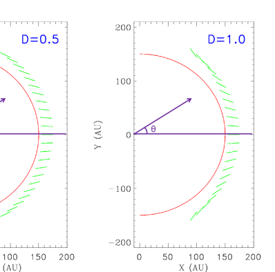
Figure 1: Representations of divergent flows from a distance of 150 AU (red line) for divergence parameters D=0.5 and D=1.0.

We define our flow in a coordinate system with the Sun at the origin and the x-axis pointing in the upwind direction of the ISM flow (i.e., the stagnation axis), as in Figure 1. For our flow from the outer heliosheath, we define an outer boundary at a distance of 150 AU, as this is roughly the distance to the heliopause. The most important difference between the outer heliosheath flow and that of the ISM is the divergence of the flow around the heliopause. If $\psi$ is the angle of the flow from the x-axis, then we define a divergence parameter $D$ such that $\psi=D\times\theta$, with $\theta$ being the angle defined in Figure 1. In practice, we assume a maximum value of $\psi=80^{\circ}$ regardless of $D$. Figure 1 shows the flow patterns associated with $D=0.5$ and $D=1.0$.

In order to illustrate how $D$ affects the shape of a He beam observed at 1 AU, we use a simple flow model in two-dimensions, where the flow from the outer boundary is assumed to be affected only by solar gravity, and the flow is modeled using a routine that computes particle trajectories using simple numerical integration (e.g., Wood et al. 2002). We assume the velocity distribution function (VDF) at the outer boundary (at $r=150$ AU) is Maxwellian. We then compute the resulting particle distribution observed at (X,Y)=(1,0) in the coordinate system shown in Figure 1, where for simplicity we are assuming the observer is on the stagnation axis at 1 AU.

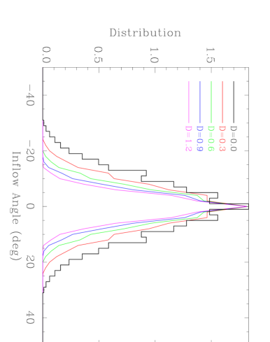
Figure 2: Models of the He distribution observed at (X,Y)=(1,0), assuming a divergent flow from 150 AU with $V=20$ km s^-1, $T=10^{4}$ K, and five values for the divergence parameter, in the range $D=0.0-1.2$.

The black line in Figure 2 shows the observed distribution for a flow with $V=20$ km s^-1 and $T=10^{4}$ K, assuming no divergence (e.g., $D=0$). Limitations in the sampling resolution of the VDF in the simulation lead to some noise in the observed He distribution. Colored lines in Figure 2 show how the observed distribution narrows as $D$ is increased from 0 to 1.2. Beam widths, $W$, can be quantified as the full-width-at-half-maxima of Gaussians fitted to the distributions. In Figure 2, increasing $D$ from 0 to 1.2 leads to a decrease in width from $W=24.3^{\circ}$ to $W=11.4^{\circ}$.

The decrease of $W$ with increasing $D$ happens because as the observer looks farther from the stagnation axis (i.e, as $\theta$ increases), the flow at the boundary becomes directed further away from the line of sight relative to a laminar flow, the result being a faster decrease in observed flux with $\theta$ compared to a laminar flow, and therefore a narrower He beam. Decreasing $T$ would also naturally narrow the observed distributions, as the VDF at the source is narrower. Thus, if $D$ is increased, one can preserve the same $W$ by increasing $T$, illlustrating how assuming a divergent flow would increase the $T=9500$ K measurement of Kubiak et al. (2016) towards a more reasonable value. The width will also be affected by the velocity $V$, because as $V$ is decreased there is more dispersion introduced into the observed distribution by the Sun’s gravitational effects.

3 Remotely Measuring Flow Divergence

In order to further explore the dependence of $W$ on $D$, $T$, and $V$; a number of trials like those in Figure 2 are computed, assuming a range of $D$, $T$, and $V$ values, and measuring the $W$ values associated with them. The observed ($D$,$T$,$V$,$W$) points are fitted with the following power law relation:

$$W=C\left(\frac{V}{20}\right)^{\alpha}\left(\frac{T}{10^{4}}\right)^{\beta}\left(D+1\right)^{\gamma},$$ (1)

with $V$ in km s^-1 and $T$ in K. A least squares analysis is used to determine the values of $C$, $\alpha$, $\beta$, and $\gamma$ that lead to the best fit to the measurements. The best fit is shown in Figure 3, with $C=24.1^{\circ}$, $\alpha=-0.84$, $\beta=0.52$, and $\gamma=-0.91$. The quality of the fit demonstrates that the power law relation provides a reasonable approximation for how $W$ depends on $D$, $T$, and $V$.

Figure 3: Comparison between the He distribution widths predicted by the power law relation between $W$, $V$, $T$, and $D$ in equation (1); and the observed widths based on numerical models, like those in Figure 2.

Based on equation (1), the Kubiak et al. (2016) fit to the secondaries, ($D$,$T$,$V$)=(0,9500,11.3), suggests a He beam width of $W=37.9^{\circ}$ in the context of our simple 2-D model geometry. Global heliospheric models suggest $V\approx 9$ km s^-1 and $T\approx 21,000$ K for the outer heliosheath (Kubiak et al. 2014; Izmodenov & Alexashov 2015). Assuming these values for $V$ and $T$, we can use equation (1) to compute the value of $D$ necessary to recover the $W=37.9^{\circ}$ value that is crudely representative of the IBEX measurements. The resulting divergence is $D=0.94$. We therefore would expect that the IBEX data could also be reasonably well fit by a flow with parameters ($D$,$T$,$V$)=(0.94,21000,9), with a temperature that is more plausible for the outer heliosheath than the $T=9500$ K measurement of Kubiak et al. (2016).

Obviously, an actual fit to the IBEX data needs to be performed to verify that such a flow can reproduce the observations. Nevertheless, this exercise illustrates how the He secondaries may provide a way to actually detect and measure the divergence of the ISM flow around the heliopause. This point becomes even more valid if it can be demonstrated that a $D>0$ flow demonstrably fits the IBEX data better than a $D=0$ flow.

In future modeling of IBEX data using a parametrized divergent flow, the model will have to be fully 3-D, and it will be necessary to address the question of how to deal with asymmetries in the flow caused by the ISM magnetic field (e.g., Kubiak et al. 2014; Izmodenov & Alexashov 2015). One approach is to simply allow the flow axis direction to differ from the ISM flow direction, as Kubiak et al. (2016) have done. The apparent deflection of the secondary He flow from the primary flow in a manner consistent with the ISM field orientation is in fact one of the biggest lines of argument in favor of the “Warm Breeze” neutrals originating in the outer heliosheath (Kubiak et al. 2016).

However, it is worth noting that the term “deflection” is not the most physically accurate description of what is going on, neither for the secondary He neutrals, nor for the secondary H neutrals studied by Lallement et al. (2005). There are, after all, no neutrals that are actually being physically deflected at the heliopause. Instead, what is happening is an asymmetry in the divergence of the flow, which yields an average velocity vector for the flow inside the heliopause that is shifted from the original ISM flow direction. With a parametrized divergent flow it should actually be possible to keep the central flow axis fixed to the flow direction of the primary ISM flow component, but to allow the divergence to vary with direction in some smooth fashion, relative to a plane defined by the ISM magnetic field and flow directions. Such an approach could in principle provide a more physically realistic description of the flow without increasing the number of free parameters of the fit.

Regardless of how one implements a parametrized divergent flow model, it is worthwhile to keep in mind that it will still only be an approximation for the actual complex flow pattern. It will always be useful to use sophisticated global heliospheric models (e.g, Müller et al. 2013; Izmodenov & Alexashov 2015) to provide direct predictions for the He secondary flow properties observed by IBEX. Such models provide the most realistic descriptions of the flow pattern in the outer heliosheath. However, a parametrized flow description is necessary to perform model-independent fits to IBEX data, and in such fitting the methodology proposed here should be preferable to the “laminar flow from infinity” approximation.

Support for this project was provided by NASA award NNH16AC40I to the Naval Research Laboratory.

References

Bzowski, M., Kubiak, M. A, Hłond, M., et al. 2014, A&A, 569, A8

Bzowski, M., Kubiak, M. A, Möbius, E., et al. 2012, ApJS, 198, 12

Izmodenov, V. V., & Alexashov, D. B. 2015, ApJS, 220, 32

Kubiak, M. A., Bzowski, M., Sokól, J. M., et al. 2014, ApJS, 213, 29

Kubiak, M. A., Swaczyna, P., Bzowski, M., et al. 2016, ApJS, 223, 25

Lallement, R., Quémerais, E., Bertaux, J. L., et al. 2005, Science, 307, 1447

McComas, D. J., Allegrini, G., Bochsler, P., et al. 2009, Space Sci. Rev., 146, 11

McComas, D. J., Bzowski, M., Frisch, P., et al. 2015, ApJ, 801, 28

Müller, H. -R., Bzowski, M., Möbius, E., & Zank, G. P. 2013, in Solar Wind 13, ed. G. P. Zank, et al. (New York: AIP, Vol. 1539), 348

Witte, M. 2004, A&A, 426, 835

Wood, B. E., Karovska, M., & Raymond, J. C. 2002, ApJ, 575, 1057

Wood, B. E., Müller, H. -R., & Witte, M. 2015, ApJ, 801, 62

Zank, G. P., Heerikhuisen, J., Wood, B. E., et al. 2013, ApJ, 763, 20