\newsiamremark

remarkRemark \newsiamremarkhypothesisHypothesis \newsiamthmclaimClaim \headersStrong convergence analysis for Langevin Dynamics X. Li and A. Telatovich

Strong Convergence Analysis for Numerical Methods for the Langevin Dynamics Model and Higher-order Operator-splitting Schemes thanks: Submitted to the editors DATE. \fundingThe research of X. Li is funded by NSF grant NSF Grant DMS-1522617 and DMS-1619661.

Xiantao Li (, http://personal.psu.edu/xxl12/). xli@math.psu.edu    Adam Telatovich22footnotemark: 2 (, ). atelatov@umd.edu adam.telatovich@gmail.com
Abstract

We provide the analysis of the strong convergence of some widely implemented methods for the Langevin dynamics model with additive noise. We show that a direct splitting of deterministic and random terms, including the symmetric splitting methods, only offers strong convergence of order 1. We present some new methods with higher order strong convergence. The new class of methods are operator-splitting schemes, constructed based on the Kunita’s solution representation for stochastic differential equations. We present stochastic algorithms with strong orders up to 3. Both mathematical analysis and numerical evidence are provided to verify the desired order of accuracy. We also examine the over-damped and under-damped limits of some of the new methods.

keywords:
stochastic differential equations, Langevin dynamics, operator-splitting methods, Itô-Taylor expansion
{AMS}

60H35, 65C30

1 Introduction

The Langevin dynamics (LD) equation plays a fundamental role in the modeling of many complex dynamical systems subject to random noise. In its simplest form, it can be expressed as the Newton’s equations of motion with added frictional and random forces, which are usually introduced to model the influence of the surrounding environment, and posed to satisfy the fluctuation-dissipation theorem.

It does not come as a surprise that such equations only have explicit solutions in very rare cases. In general, approximate solutions have to be constructed at discrete time steps. As a system of stochastic differential equations (SDE), there are various classical methods for approximating the solutions [11]. However, low order methods, such as the Euler-Maruyama method, often do not have sufficient accuracy for accurate predictions. On the other hand, higher order methods that are constructed based on direct expansions of solutions (Itô-Taylor expansions) usually involve high order derivatives of the drift and diffusion coefficients, which makes the implementation rather difficult. For instance, for bio-molecular models [28], this implies that one has to compute the derivatives of the inter-molecular forces, which typically is not plausible. Extensions of Runge-Kutta methods, due to the many evaluations of the drift and diffusion terms at intermediate stages, have been largely neglected in the molecular simulation community. In molecular models [16, Chapter 7], instead of using Runge-Kutta methods [26], operator-splitting schemes have been more widely implemented. Such algorithms, especially with applications to molecular dynamics simulations, have been treated extensively in [13, 16], where many theoretical and practical aspects have been discussed. The idea is to separate out terms on the right hand side and form two or more SDEs, each of which can be solved explicitly. This is denoted by an [ABO] notation in [13]. Many existing methods can be recast into this form [14, 15, 2, 4, 21, 3]. One particular advantage of the splitting methods is that they are very easy to implement, since each substep can be carried out exactly. The splitting methods can also be designed to better sample the equilibrium averages. Another important approach is based on solving the coordinate and momentum equations consecutively. For example, one can start by assuming the coordinates remain constant, and integrate out the momentum equation exactly. Then using this solution for the momentum, one can integrate the first equation and obtain an updated coordinate for the next step. These two steps can be written in an operator splitting form. But a further correction can be made by assuming the force is linear in time, constructed using the coordinates at the current and next steps. This led to the stochastic velocity Verlet method (SVV) [6, 1, 33], which has been implemented in simulation packages, e.g., TINKER [25]. Other integration methods can also be found in the literature [34, 30, 19, 21, 23].

On the theoretical side, the fundamental issue of the numerical accuracy has been thoroughly discussed in [13, 5]. In particular, the weak convergence of the numerical solution has been rigorously proved in [17]. Such analysis is crucial when the approximation methods are used to sample the corresponding equilibrium statistics. This is particularly useful when the averages of certain quantities are of interest. On the other hand, to the best of our knowledge, the theoretical analysis of strong convergence has not been fully studied. Strong convergence ensures the accuracy in terms of individual realizations and solutions at transient stages [27]. Such notation of accuracy would be useful in non-equilibrium simulations, such as non-equilibrium molecular dynamics (NEMD) simulations, which have been very useful in the study of transport processes [9, 20, 10, 8]. Strong convergence usually implies weak convergence, but not vice versa. Typically, strong convergence can be examined by comparing to the Itô-Taylor expansion. Therefore, the fact that the splitting methods discussed in the literature often do not involve multiple Itô integrals of order 2 or higher is already an indication that those methods are only of strong order 1 or less, regardless of how the operators are split up and how many fractional steps are involved.

This paper will primarily focus on this theoretical aspect. In the first half, we analyze two widely used methods, namely the SVV and a naive splitting method. In the second half, we present several new operator splitting methods with higher strong order. Our starting point for the new methods is the solution representation by Kunita [12]. Written formally as an operator exponential form, the differential operator is expressed in terms of the commutators involving the differential operators associated with the drift and diffusion coefficients, along with multiple Itô integrals. Intuitively, we can make truncations at various levels, yielding approximation methods of increasing order. Such truncation schemes have been used in [22] for one-dimensional stochastic differential equations as a starting point to construct robust algorithms for scalar SDEs with multiplicative noise. It was demonstrated that such algorithms can preserve the non-negativity of the solution. In this paper, we extend the applications of these truncations to the Langevin dynamics, introducing truncations of the solution operator, and obtaining approximate solutions that can be written as solutions of ODEs, for which many efficient methods exist. We choose the well established operator splitting methods for these ODEs, yielding new operator splitting schemes for the Langevin dynamics model. With direct mathematical analysis and numerical tests, we verify that these methods have strong order 2 and 3. They can be used as highly accurate numerical tools to study stochastic dynamics modeled by Langevin dynamics. No derivatives of the force function are required for the order 2 splitting method, and only first order derivatives are needed for the order 3 splitting method.

The rest of the paper is organized as follows. Section 2 presents the basic theory for strong convergence. In Section 3, we analyze the convergence of some existing numerical methods. In Section 4, we introduce the new class of operator splitting schemes based on the truncations of the Kunita’s solution operator and examined the strong order of accuracy. Section 6 contains numerical tests that will demonstrate the expected order of convergence. Section 5 contains our proofs of the convergence results we presented in Section 3 and Section 4, and Section 8 is the Appendix where we derive the Itô-Taylor expansions for the Langevin model.

2 The basic theory

This paper is mainly concerned with the Langevin dynamics model with n𝑛n spacial dimensions,

(1) {dx=vdt,dv=f(x)dtΓvdt+σdWt,\left\{\begin{aligned} dx=&vdt,\\ dv=&f(x)dt-\Gamma vdt+\sigma dW_{t},\end{aligned}\right.

where x=(x1,,xn),v=(v1,,vn)nformulae-sequence𝑥superscript𝑥1superscript𝑥𝑛𝑣superscript𝑣1superscript𝑣𝑛superscript𝑛x=(x^{1},\dots,x^{n}),v=(v^{1},\dots,v^{n})\in\mathbb{R}^{n} can be interpreted as position and velocity components respectively, W(t)=(W1(t),,Wn(t))n𝑊𝑡superscript𝑊1𝑡superscript𝑊𝑛𝑡superscript𝑛W(t)=(W^{1}(t),\dots,W^{n}(t))\in\mathbb{R}^{n} is the standard nlimit-from𝑛n-dimensional Brownian motion and 0tT0𝑡𝑇0\leq t\leq T. W(t)superscript𝑊𝑡W^{\prime}(t) represents white noise in time. Assume the function f=f(x):nn:𝑓𝑓𝑥superscript𝑛superscript𝑛f=f(x):\mathbb{R}^{n}\rightarrow\mathbb{R}^{n}, representing the conservative force (for example, the Morse potential), has bounded second derivatives. Here we will consider the case where σ𝜎\sigma and ΓΓ\Gamma are constant n×n𝑛𝑛n\times n matrices which we assume satisfy the fluctuation dissipation theorem,

(2) σσT=2ΓkBT,𝜎superscript𝜎𝑇2Γsubscript𝑘𝐵𝑇\sigma\sigma^{T}=2\Gamma k_{B}T,

where kBsubscript𝑘𝐵k_{B} is Boltzman’s constant, σTsuperscript𝜎𝑇\sigma^{T} denotes the transpose of σ𝜎\sigma, and T𝑇T represents the temperature of the system. In particular, the noise is additive, and as a consequence, (1) may be interpreted as either an Itô or Stratonovich SDE. For particle dynamics, typically n=3N𝑛3𝑁n=3N, with N𝑁N being the total number of particles.

We can view the Langevin equation above as an example of an autonomous Itô SDE

(3) dzt=a(zt)dt+bdWt,𝑑subscript𝑧𝑡𝑎subscript𝑧𝑡𝑑𝑡𝑏𝑑subscript𝑊𝑡\displaystyle dz_{t}=a(z_{t})dt+bdW_{t},

where zt=(xt,vt)subscript𝑧𝑡subscript𝑥𝑡subscript𝑣𝑡z_{t}=(x_{t},v_{t}), and a,b𝑎𝑏a,b are the respective drift and (constant) diffusion terms, given here by

(4) a=(vf(x)Γv)2n, b=(0σ)2n×n.formulae-sequence𝑎matrix𝑣𝑓𝑥Γ𝑣superscript2𝑛 𝑏matrix0𝜎superscript2𝑛𝑛\displaystyle a=\left(\begin{matrix}v\\ f(x)-\Gamma v\end{matrix}\right)\in\mathbb{R}^{2n},\text{\quad}b=\left(\begin{matrix}0\\ \sigma\end{matrix}\right)\in\mathbb{R}^{2n\times n}.

The numerical solutions will involve Brownian increments, whose j𝑗jth component (j=1,,n𝑗1𝑛j=1,\dots,n) at the k𝑘kth step (k=0,,nT1𝑘0subscript𝑛𝑇1k=0,\dots,n_{T}-1) are ΔtN(0,1)Δ𝑡𝑁01\sqrt{{\Delta t}}N(0,1) random variables ΔWkj:=Wtk+1jWtkjassignΔsuperscriptsubscript𝑊𝑘𝑗superscriptsubscript𝑊subscript𝑡𝑘1𝑗superscriptsubscript𝑊subscript𝑡𝑘𝑗\Delta W_{k}^{j}:=W_{t_{k+1}}^{j}-W_{t_{k}}^{j}, where {tk}k=1nTsuperscriptsubscriptsubscript𝑡𝑘𝑘1subscript𝑛𝑇\{t_{k}\}_{k=1}^{n_{T}} is the uniform discretization tk=kΔtsubscript𝑡𝑘𝑘Δ𝑡t_{k}=k{\Delta t} of a time interval [0,T]0𝑇[0,T] with uniform step size Δt=tk+1tkΔ𝑡subscript𝑡𝑘1subscript𝑡𝑘{\Delta t}=t_{k+1}-t_{k}. In vector form, we write ΔWk=(ΔWk1,,ΔWkn)Δsubscript𝑊𝑘Δsuperscriptsubscript𝑊𝑘1Δsuperscriptsubscript𝑊𝑘𝑛\Delta W_{k}=(\Delta W_{k}^{1},\dots,\Delta W_{k}^{n}). The components ΔWkiΔsuperscriptsubscript𝑊𝑘𝑖\Delta W_{k}^{i} and ΔWkjΔsuperscriptsubscript𝑊𝑘𝑗\Delta W_{k}^{j} are pairwise independent for each step k𝑘k, and the increments ΔWkjΔsuperscriptsubscript𝑊𝑘𝑗\Delta W_{k}^{j} and ΔWljΔsuperscriptsubscript𝑊𝑙𝑗\Delta W_{l}^{j} are independent for each component j𝑗j.

A discrete time approximation Y=YΔt𝑌superscript𝑌Δ𝑡Y=Y^{{\Delta t}} of X𝑋X with uniform step size ΔtΔ𝑡{\Delta t} converges with strong order γ{0.5,1,1.5,2,}𝛾0.511.52\gamma\in\{0.5,1,1.5,2,\dots\} at time T>0𝑇0T>0 provided that there are constants C𝐶C and Δ>0Δ0\Delta>0 such that

(5) 𝔼(sup0knT|X(kΔt)Y(kΔt)|)CΔtγ for all 0<Δt<Δ.𝔼subscriptsupremum0𝑘subscript𝑛𝑇𝑋𝑘Δ𝑡𝑌𝑘Δ𝑡𝐶Δsuperscript𝑡𝛾 for all 0Δ𝑡Δ\mathbb{E}\left(\sup_{0\leq k\leq n_{T}}|X(k{\Delta t})-Y(k{\Delta t})|\right)\leq C{\Delta t}^{\gamma}\text{\quad for all }0<{\Delta t}<\Delta.

The notation 𝔼()𝔼\mathbb{E}(\cdot) denotes the usual expectation of a random variable on a probability space (Ω,,P)Ω𝑃(\Omega,\mathcal{F},P). The random variables X,Y𝑋𝑌X,Y are driven by the same process Wtsubscript𝑊𝑡W_{t}. Clearly, strong convergence is related to the convergence of paths.

Remark 2.1.

We point out that the definition above actually means that the convergence is uniform over the entire time interval [0,T]0𝑇[0,T], whereas the definition given in [11, eq. 9.6.3] means convergence at the terminal time T𝑇T:

(6) 𝔼(|X(T)Y(T)|)CΔtγ for all 0<Δt<Δ.𝔼𝑋𝑇𝑌𝑇𝐶Δsuperscript𝑡𝛾 for all 0Δ𝑡Δ\mathbb{E}\left(|X(T)-Y(T)|\right)\leq C{\Delta t}^{\gamma}\text{\quad for all }0<{\Delta t}<\Delta.

We will use the former definition of strong convergence instead of the latter, showing preference for uniform estimates over point-wise estimates.

3 Analysis of some existing methods

3.1 Itô-Taylor expansion of the solution

To construct an algorithm with certain strong order of accuracy, a direct comparison has to be made with the Itô-Taylor expansion of the exact solution [11]. With direct, but involved calculations, we have obtained such expansions for the Langevin dynamics model (1), given as follows,

Lemma 1.

The strong Itô-Taylor approximations of order 1, 2 and 3 for the Langevin equation (1) with additive noise are one-step methods given at step k+1𝑘1k+1, for k=0,1,,nT1𝑘01subscript𝑛𝑇1k=0,1,\dots,n_{T}-1, respectively, by

(7) (xk+1vk+1)matrixsubscript𝑥𝑘1subscript𝑣𝑘1\displaystyle\left(\begin{matrix}x_{k+1}\\ v_{k+1}\end{matrix}\right) =(xkvk)+(vkf(xk)Γvk)Δt+(0σΔWk)+H.O.T.,formulae-sequenceabsentmatrixsubscript𝑥𝑘subscript𝑣𝑘matrixsubscript𝑣𝑘𝑓subscript𝑥𝑘Γsubscript𝑣𝑘Δ𝑡matrix0𝜎Δsubscript𝑊𝑘𝐻𝑂𝑇\displaystyle=\left(\begin{matrix}x_{k}\\ v_{k}\end{matrix}\right)+\left(\begin{matrix}v_{k}\\ f(x_{k})-\Gamma v_{k}\end{matrix}\right){\Delta t}+\left(\begin{matrix}0\\ \sigma\Delta W_{k}\end{matrix}\right)+H.O.T.,
(xk+1vk+1)matrixsubscript𝑥𝑘1subscript𝑣𝑘1\displaystyle\left(\begin{matrix}x_{k+1}\\ v_{k+1}\end{matrix}\right) =(xkvk)+(vkf(xk)Γvk)Δt+(0σΔWk)absentmatrixsubscript𝑥𝑘subscript𝑣𝑘matrixsubscript𝑣𝑘𝑓subscript𝑥𝑘Γsubscript𝑣𝑘Δ𝑡matrix0𝜎Δsubscript𝑊𝑘\displaystyle=\left(\begin{matrix}x_{k}\\ v_{k}\end{matrix}\right)+\left(\begin{matrix}v_{k}\\ f(x_{k})-\Gamma v_{k}\end{matrix}\right){\Delta t}+\left(\begin{matrix}0\\ \sigma\Delta W_{k}\end{matrix}\right)
+(f(xk)Γvkx(f(xk))vkΓf(xk)+Γ2vk)Δt22+(σI(J,0),k(Δt)ΓσI(J,0),k(Δt))+H.O.T.,formulae-sequencematrix𝑓subscript𝑥𝑘Γsubscript𝑣𝑘subscript𝑥𝑓subscript𝑥𝑘subscript𝑣𝑘Γ𝑓subscript𝑥𝑘superscriptΓ2subscript𝑣𝑘Δsuperscript𝑡22matrix𝜎subscript𝐼𝐽0𝑘Δ𝑡Γ𝜎subscript𝐼𝐽0𝑘Δ𝑡𝐻𝑂𝑇\displaystyle+\left(\begin{matrix}f(x_{k})-\Gamma v_{k}\\ \nabla_{x}\left(f(x_{k})\right)v_{k}-\Gamma f(x_{k})+\Gamma^{2}v_{k}\end{matrix}\right)\frac{{\Delta t}^{2}}{2}+\left(\begin{matrix}\sigma I_{(J,0),k}({\Delta t})\\ -\Gamma\sigma I_{(J,0),k}({\Delta t})\end{matrix}\right)+H.O.T.,
(xk+1vk+1)matrixsubscript𝑥𝑘1subscript𝑣𝑘1\displaystyle\left(\begin{matrix}x_{k+1}\\ v_{k+1}\end{matrix}\right) =(xkvk)+(vkf(xk)Γvk)Δt+(0σΔWk)absentmatrixsubscript𝑥𝑘subscript𝑣𝑘matrixsubscript𝑣𝑘𝑓subscript𝑥𝑘Γsubscript𝑣𝑘Δ𝑡matrix0𝜎Δsubscript𝑊𝑘\displaystyle=\left(\begin{matrix}x_{k}\\ v_{k}\end{matrix}\right)+\left(\begin{matrix}v_{k}\\ f(x_{k})-\Gamma v_{k}\end{matrix}\right){\Delta t}+\left(\begin{matrix}0\\ \sigma\Delta W_{k}\end{matrix}\right)
+(f(xk)Γvkx(f(xk))vkΓf(xk)+Γ2vk)Δt22+(σI(J,0),k(Δt)ΓσI(J,0),k(Δt))matrix𝑓subscript𝑥𝑘Γsubscript𝑣𝑘subscript𝑥𝑓subscript𝑥𝑘subscript𝑣𝑘Γ𝑓subscript𝑥𝑘superscriptΓ2subscript𝑣𝑘Δsuperscript𝑡22matrix𝜎subscript𝐼𝐽0𝑘Δ𝑡Γ𝜎subscript𝐼𝐽0𝑘Δ𝑡\displaystyle+\left(\begin{matrix}f(x_{k})-\Gamma v_{k}\\ \nabla_{x}\left(f(x_{k})\right)v_{k}-\Gamma f(x_{k})+\Gamma^{2}v_{k}\end{matrix}\right)\frac{{\Delta t}^{2}}{2}+\left(\begin{matrix}\sigma I_{(J,0),k}({\Delta t})\\ -\Gamma\sigma I_{(J,0),k}({\Delta t})\end{matrix}\right)
+(x(f(xk))vkΓf(xk)+Γ2vkx[x(f(xk))vk]vkΓx(f(xk))vk)Δt33!matrixsubscript𝑥𝑓subscript𝑥𝑘subscript𝑣𝑘Γ𝑓subscript𝑥𝑘superscriptΓ2subscript𝑣𝑘subscript𝑥subscript𝑥𝑓subscript𝑥𝑘subscript𝑣𝑘subscript𝑣𝑘Γsubscript𝑥𝑓subscript𝑥𝑘subscript𝑣𝑘Δsuperscript𝑡33\displaystyle+\left(\begin{matrix}\nabla_{x}\left(f(x_{k})\right)v_{k}-\Gamma f(x_{k})+\Gamma^{2}v_{k}\\ \nabla_{x}[\nabla_{x}(f(x_{k}))v_{k}]v_{k}-\Gamma\nabla_{x}(f(x_{k}))v_{k}\end{matrix}\right)\frac{{\Delta t}^{3}}{3!}
+(0x(f(xk))(f(xk)Γvk)+Γ2(f(xk)Γvk))Δt33!matrix0subscript𝑥𝑓subscript𝑥𝑘𝑓subscript𝑥𝑘Γsubscript𝑣𝑘superscriptΓ2𝑓subscript𝑥𝑘Γsubscript𝑣𝑘Δsuperscript𝑡33\displaystyle+\left(\begin{matrix}0\\ \nabla_{x}(f(x_{k}))(f(x_{k})-\Gamma v_{k})+\Gamma^{2}(f(x_{k})-\Gamma v_{k})\end{matrix}\right)\frac{{\Delta t}^{3}}{3!}
+(ΓσI(J,0,0),k(Δt)(x(f(xk))σ+Γ2σ)I(J,0,0),k(Δt))+H.O.T.formulae-sequencematrixΓ𝜎subscript𝐼𝐽00𝑘Δ𝑡subscript𝑥𝑓subscript𝑥𝑘𝜎superscriptΓ2𝜎subscript𝐼𝐽00𝑘Δ𝑡𝐻𝑂𝑇\displaystyle+\left(\begin{matrix}-\Gamma\sigma I_{(J,0,0),k}({\Delta t})\\ \left(\nabla_{x}(f(x_{k}))\sigma+\Gamma^{2}\sigma\right)I_{(J,0,0),k}({\Delta t})\end{matrix}\right)+H.O.T.

where σjsuperscript𝜎𝑗\sigma^{j} is the j𝑗jth column of σn×m𝜎superscript𝑛𝑚\sigma\in\mathbb{R}^{n\times m}, xf(x)n×nsubscript𝑥𝑓𝑥superscript𝑛𝑛\nabla_{x}f(x)\in\mathbb{R}^{n\times n} is the gradient matrix of f(x)n𝑓𝑥superscript𝑛f(x)\in\mathbb{R}^{n} at x𝑥x, (xf(x))ij=fi(x)xjsubscriptsubscript𝑥𝑓𝑥𝑖𝑗subscript𝑓𝑖𝑥superscript𝑥𝑗(\nabla_{x}f(x))_{ij}=\frac{\partial f_{i}(x)}{\partial x^{j}}, and x[x(f(x))v]subscript𝑥subscript𝑥𝑓𝑥𝑣\nabla_{x}[\nabla_{x}(f(x))v] is the gradient matrix of xf(x)vnsubscript𝑥𝑓𝑥𝑣superscript𝑛\nabla_{x}f(x)v\in\mathbb{R}^{n} at x𝑥x. The abbreviation H.O.T. stands for Higher Order Terms (with respect to ΔtΔ𝑡{\Delta t}). For the calculations involved to derive the expansions above, the reader may refer to Section 8. Furthermore, the strong order 0.5, 1.5 and 2.5 Itô-Taylor approximations are the same as the strong order 1, 2 and 3 approximations, respectively, due to the fact that the noise is additive.

It is important to point out that I(J,0),k=(I(1,0),k,,I(n,0),k)nsubscript𝐼𝐽0𝑘subscript𝐼10𝑘subscript𝐼𝑛0𝑘superscript𝑛I_{(J,0),k}=(I_{(1,0),k},\dots,I_{(n,0),k})\in\mathbb{R}^{n} and the I(J,0,0),k=(I(1,0,0),k,,I(n,0,0),k)nsubscript𝐼𝐽00𝑘subscript𝐼100𝑘subscript𝐼𝑛00𝑘superscript𝑛I_{(J,0,0),k}=(I_{(1,0,0),k},\dots,I_{(n,0,0),k})\in\mathbb{R}^{n} are random vectors, with components I(j,0),ksubscript𝐼𝑗0𝑘I_{(j,0),k} and I(j,0,0),ksubscript𝐼𝑗00𝑘I_{(j,0,0),k} which are multiple stochastic integrals, given by the following formulas

(8) I(j,0),k(t)subscript𝐼𝑗0𝑘𝑡\displaystyle I_{(j,0),k}(t) =tktk+1Wsj𝑑sabsentsuperscriptsubscriptsubscript𝑡𝑘subscript𝑡𝑘1superscriptsubscript𝑊𝑠𝑗differential-d𝑠\displaystyle=\int_{t_{k}}^{t_{k+1}}W_{s}^{j}ds
I(j,0,0),k(t)subscript𝐼𝑗00𝑘𝑡\displaystyle I_{(j,0,0),k}(t) =tktk+1tksWuj𝑑u𝑑s.absentsuperscriptsubscriptsubscript𝑡𝑘subscript𝑡𝑘1superscriptsubscriptsubscript𝑡𝑘𝑠superscriptsubscript𝑊𝑢𝑗differential-d𝑢differential-d𝑠\displaystyle=\int_{t_{k}}^{t_{k+1}}\int_{t_{k}}^{s}W_{u}^{j}duds.

The quantities ΔWkΔsubscript𝑊𝑘\Delta W_{k}, I(J,0),ksubscript𝐼𝐽0𝑘I_{(J,0),k} and I(J,0,0),ksubscript𝐼𝐽00𝑘I_{(J,0,0),k} are independent Gaussian random variables, whose means and variances do not depend on k𝑘k due to translation invariance, and they have the same distributions, respectively, as the following random variables:

(9) ΔW:=WΔt, I(j,0):=0ΔtWsj𝑑s, and I(j,0,0):=0Δt0sWuj𝑑u𝑑s.formulae-sequenceassignΔ𝑊subscript𝑊Δ𝑡formulae-sequenceassign subscript𝐼𝑗0superscriptsubscript0Δ𝑡superscriptsubscript𝑊𝑠𝑗differential-d𝑠assign and subscript𝐼𝑗00superscriptsubscript0Δ𝑡superscriptsubscript0𝑠superscriptsubscript𝑊𝑢𝑗differential-d𝑢differential-d𝑠\Delta W:=W_{{\Delta t}},\text{\quad}I_{(j,0)}:=\int_{0}^{{\Delta t}}W_{s}^{j}ds,\text{\quad and\quad}I_{(j,0,0)}:=\int_{0}^{{\Delta t}}\int_{0}^{s}W_{u}^{j}duds.

The expansions (7) reduces to the usual Taylor expansions when σ=0𝜎0\sigma=0. We refer the readers to Section 8 or to [11] for the detailed explanation of the notations. How the terms in the expansion are retained is determined by an estimate on the variance of each term, and how they accumulate in time [11]. The additive noise has the desirable effect that several terms vanish in the Itô Taylor expansion.

One-step numerical schemes can be directly obtained from the Itô-Taylor expansion (7). For example, by neglecting the high order terms (H.O.T.) in the first expansion, one obtains the familiar Euler-Maruyama (EM) method, which in this case has strong order 1. It is tempting to make truncations for the order 2 and 3 expansions. However, those direct expansions involve higher order derivatives of f(x)𝑓𝑥f(x), and they may not be easy to implement. Specifically, the order 2 expansion requires computing xfsubscript𝑥𝑓\nabla_{x}f and the order 3 expansion requires both xfsubscript𝑥𝑓\nabla_{x}f and x2fsuperscriptsubscript𝑥2𝑓\nabla_{x}^{2}f. Therefore, we only use these expansion as a guideline to prove strong order convergence and construct algorithms with high strong order, in light of the theoretical analysis (Theorem 11.5.1 [11]).

3.2 Some existing splitting methods

A natural approximation of (1) can be obtained by splitting the equation into several subproblems, each of which can be solved exactly. A wide variety of splitting methods have been discussed in [13] that have this flavor. For example, we may consider to split the Langevin equation as follows,

(10) {x=vv=0,\left\{\begin{aligned} x^{\prime}=&v\\ v^{\prime}=&0,\end{aligned}\right.

and

(11) {x=0v=f(x)Γv+σW(t).\left\{\begin{aligned} x^{\prime}=&0\\ v^{\prime}=&f(x)-\Gamma v+\sigma W^{\prime}(t).\end{aligned}\right.

Both of these equations have explicit solutions. The solution steps can be denoted by abstract operators A𝐴A and B𝐵B, respectively, and approximations can be obtained by following the operations, e.g., AB𝐴𝐵AB, A2BA2𝐴2𝐵𝐴2\frac{A}{2}B\frac{A}{2}, etc [13]. Unfortunately, the strong accuracy of these methods is very limited, as shown by the following theorem.

Theorem 2.

The symmetric and non-symmetric splitting methods,

exp(A/2)exp(B)exp(A/2) and exp(A)exp(B),𝐴2𝐵𝐴2 and 𝐴𝐵\exp(A/2)\exp(B)\exp(A/2)\text{\quad and\quad}\exp(A)\exp(B),

respectively, have strong order 1.

The proof will be postponed to Section 5.2.


3.3 The stochastic velocity-Verlet (SVV) method

Another widely implemented scheme is the stochastic velocity-Verlet’s (SVV) method [33], as we mentioned in the introduction. This method starts with an assumption that x(t)𝑥𝑡x(t) remains as a constant, and integrates the second equation in (1) exactly, giving rise to,

(12) v(t)=c0(t)vk+c1(t)f(xk)+tkteΓ(ts)σ𝑑Ws,𝑣𝑡subscript𝑐0𝑡subscript𝑣𝑘subscript𝑐1𝑡𝑓subscript𝑥𝑘superscriptsubscriptsubscript𝑡𝑘𝑡superscript𝑒Γ𝑡𝑠𝜎differential-dsubscript𝑊𝑠v(t)=c_{0}(t)v_{k}+c_{1}(t)f(x_{k})+\int_{t_{k}}^{t}e^{-\Gamma(t-s)}\sigma dW_{s},

where tkttk+1subscript𝑡𝑘𝑡subscript𝑡𝑘1t_{k}\leq t\leq t_{k+1}, the time-dependent coefficients c0,c1subscript𝑐0subscript𝑐1c_{0},c_{1} are given by,

(13) c0(t)subscript𝑐0𝑡\displaystyle c_{0}(t) =eΓt,absentsuperscript𝑒Γ𝑡\displaystyle=e^{-\Gamma t},
c1(t)subscript𝑐1𝑡\displaystyle c_{1}(t) =Γ1(Ic0(t)),absentsuperscriptΓ1𝐼subscript𝑐0𝑡\displaystyle=\Gamma^{-1}(I-c_{0}(t)),

I𝐼I denotes the n×n𝑛𝑛n\times n identity matrix and eΓtsuperscript𝑒Γ𝑡e^{-\Gamma t} is a matrix exponential. (For a derivation of this formula, see Section 5.2.)

With this approximation of v(t)𝑣𝑡v(t), one can now turn to the first equation, and integrate. This gives,

(14) xk+1=xk+c1(Δt)vk+c2(Δt)f(xk)+tktk+1tkteΓ(ts)σ𝑑Ws𝑑t.subscript𝑥𝑘1subscript𝑥𝑘subscript𝑐1Δ𝑡subscript𝑣𝑘subscript𝑐2Δ𝑡𝑓subscript𝑥𝑘superscriptsubscriptsubscript𝑡𝑘subscript𝑡𝑘1superscriptsubscriptsubscript𝑡𝑘𝑡superscript𝑒Γ𝑡𝑠𝜎differential-dsubscript𝑊𝑠differential-d𝑡x_{k+1}=x_{k}+c_{1}({\Delta t})v_{k}+c_{2}({\Delta t})f(x_{k})+\int_{t_{k}}^{t_{k+1}}\int_{t_{k}}^{t}e^{-\Gamma(t-s)}\sigma dW_{s}dt.

Here the new coefficient c2subscript𝑐2c_{2} is given by,

(15) c2(Δt)=tktk+ΔtΓ1(IeΓs)𝑑s.subscript𝑐2Δ𝑡superscriptsubscriptsubscript𝑡𝑘subscript𝑡𝑘Δ𝑡superscriptΓ1𝐼superscript𝑒Γ𝑠differential-d𝑠c_{2}({\Delta t})=\int_{t_{k}}^{t_{k}+{\Delta t}}\Gamma^{-1}(I-e^{-\Gamma s})ds.

One might stop here and accept the position and velocity values. But in SVV one uses the updated position value and approximate the function f𝑓f by a linear function,

(16) f(x(t))f(x(0))+(f(x(Δt))f(x(0)))tΔt.𝑓𝑥𝑡𝑓𝑥0𝑓𝑥Δ𝑡𝑓𝑥0𝑡Δ𝑡f(x(t))\approx f(x(0))+\frac{\big{(}f(x({\Delta t}))-f(x(0))\big{)}t}{{\color[rgb]{0,0,0}{\Delta t}}}.

With this approximation, one can integrate the velocity equation again. One finds that,

(17) vk+1=c0(Δt)vk+c1(Δt)f(xk)+c2(Δt)(f(xk+1)f(xk))+0ΔteΓ(Δts)σ𝑑Ws.subscript𝑣𝑘1subscript𝑐0Δ𝑡subscript𝑣𝑘subscript𝑐1Δ𝑡𝑓subscript𝑥𝑘subscript𝑐2Δ𝑡𝑓subscript𝑥𝑘1𝑓subscript𝑥𝑘superscriptsubscript0Δ𝑡superscript𝑒ΓΔ𝑡𝑠𝜎differential-dsubscript𝑊𝑠v_{k+1}=c_{0}{\color[rgb]{0,0,0}({\Delta t})}v_{k}+c_{1}{\color[rgb]{0,0,0}({\Delta t})}f(x_{k})+c_{2}{\color[rgb]{0,0,0}({\Delta t})}\big{(}f(x_{k+1})-f(x_{k})\big{)}+\int_{0}^{\Delta t}e^{-\Gamma({\Delta t}-s)}\sigma dW_{s}.

Equations (14) and (17) form the basis for the SVV method. The formulas can be repeated, and at each step, the function f𝑓f is evaluated only once at each step, which is typically viewed as a considerable advantage. As we will prove, this algorithm has second order strong accuracy.

Theorem 3.

The SVV algorithm has strong order 2.

A brief proof can be found in Section 5.1. To the best of our knowledge, this is a new theoretical result.

4 New operator-splitting algorithm with higher order strong convergence

Here we propose new splitting algorithms. Our starting point is the Kunita’s solution operator [12]. In particular, for the standard SDE written in the differential form,

(18) dzt=a(zt)dt+b(zt)dWt, z(0)=z,formulae-sequence𝑑subscript𝑧𝑡𝑎subscript𝑧𝑡𝑑𝑡𝑏subscript𝑧𝑡𝑑subscript𝑊𝑡 𝑧0𝑧dz_{t}=a(z_{t})dt+b(z_{t})dW_{t},\text{\quad}z(0)=z,

we define the differential operators,

(19) 𝒳0=az,𝒳j=bjz,formulae-sequencesubscript𝒳0𝑎subscript𝑧subscript𝒳𝑗superscript𝑏𝑗subscript𝑧\mathcal{X}_{0}=a\cdot\nabla_{z},\quad\mathcal{X}_{j}=b^{j}\cdot\nabla_{z},

Here ztsubscript𝑧𝑡z_{t} represents the solution at time t𝑡t and bjsuperscript𝑏𝑗b^{j} denotes the j𝑗jth column of b𝑏b. Then the exact solution of the SDE can be formally expressed as,

(20) zt=exp(Dt)z,subscript𝑧𝑡subscript𝐷𝑡𝑧z_{t}=\exp(D_{t})z,

where, by [22, eq. (2.5)], for t=Δt𝑡Δ𝑡t={\Delta t} we have,

(21) DΔtsubscript𝐷Δ𝑡\displaystyle D_{{\Delta t}} =Δt𝒳0+j=1nΔWj𝒳j+12j=1n[Δt,ΔWj][𝒳0,𝒳j]absentΔ𝑡subscript𝒳0superscriptsubscript𝑗1𝑛Δsuperscript𝑊𝑗subscript𝒳𝑗12superscriptsubscript𝑗1𝑛Δ𝑡Δsuperscript𝑊𝑗subscript𝒳0subscript𝒳𝑗\displaystyle={\Delta t}\mathcal{X}_{0}+\sum_{j=1}^{n}\Delta W^{j}\mathcal{X}_{j}+\frac{1}{2}\sum_{j=1}^{n}[{\Delta t},\Delta W^{j}][\mathcal{X}_{0},\mathcal{X}_{j}]
+118j=1n[[Δt,ΔWj],Δt][[𝒳0,𝒳j],𝒳0]+118superscriptsubscript𝑗1𝑛Δ𝑡Δsuperscript𝑊𝑗Δ𝑡subscript𝒳0subscript𝒳𝑗subscript𝒳0\displaystyle+\frac{1}{18}\sum_{j=1}^{n}[[{\Delta t},\Delta W^{j}],{\Delta t}][[\mathcal{X}_{0},\mathcal{X}_{j}],\mathcal{X}_{0}]+\dots

Here, [𝒳0,𝒳j]subscript𝒳0subscript𝒳𝑗[\mathcal{X}_{0},\mathcal{X}_{j}] denotes the commutator bracket of differential operators:

(22) 𝒳0𝒳j𝒳j𝒳0,subscript𝒳0subscript𝒳𝑗subscript𝒳𝑗subscript𝒳0\mathcal{X}_{0}\mathcal{X}_{j}-\mathcal{X}_{j}\mathcal{X}_{0},

and [[𝒳0,𝒳j],𝒳0]=[𝒳0,𝒳j]𝒳0𝒳0[𝒳0,𝒳j]subscript𝒳0subscript𝒳𝑗subscript𝒳0subscript𝒳0subscript𝒳𝑗subscript𝒳0subscript𝒳0subscript𝒳0subscript𝒳𝑗[[\mathcal{X}_{0},\mathcal{X}_{j}],\mathcal{X}_{0}]=[\mathcal{X}_{0},\mathcal{X}_{j}]\mathcal{X}_{0}-\mathcal{X}_{0}[\mathcal{X}_{0},\mathcal{X}_{j}]. Higher order commutators can be defined similarly.

The corresponding terms [Δt,ΔWj]Δ𝑡Δsuperscript𝑊𝑗[{\Delta t},\Delta W^{j}] (for j=1,,n𝑗1𝑛j=1,\dots,n) are combinations of double stochastic integrals given by

(23) [Δt,ΔWkj]:=tktk+1t𝑑Wtjtktk+1Wtj𝑑t,assignΔ𝑡Δsuperscriptsubscript𝑊𝑘𝑗superscriptsubscriptsubscript𝑡𝑘subscript𝑡𝑘1𝑡differential-dsuperscriptsubscript𝑊𝑡𝑗superscriptsubscriptsubscript𝑡𝑘subscript𝑡𝑘1superscriptsubscript𝑊𝑡𝑗differential-d𝑡[{\Delta t},\Delta W_{k}^{j}]:=\int_{t_{k}}^{t_{k+1}}tdW_{t}^{j}-\int_{t_{k}}^{t_{k+1}}W_{t}^{j}dt,

and the corresponding terms [[Δt,ΔWkj],Δt]Δ𝑡Δsuperscriptsubscript𝑊𝑘𝑗Δ𝑡[[{\Delta t},\Delta W_{k}^{j}],{\Delta t}] (for j=1,,n𝑗1𝑛j=1,\dots,n) are combinations of triple stochastic integrals given by, [22, eq. (2.15)]

(24) [[Δt,ΔWkj],Δt]=118(2I(0,j,0),k2I(j,0,0),k+ΔtI(j,0),kΔtI(0,j),k).Δ𝑡Δsuperscriptsubscript𝑊𝑘𝑗Δ𝑡1182subscript𝐼0𝑗0𝑘2subscript𝐼𝑗00𝑘Δ𝑡subscript𝐼𝑗0𝑘Δ𝑡subscript𝐼0𝑗𝑘[[{\Delta t},\Delta W_{k}^{j}],{\Delta t}]=\frac{1}{18}(2I_{(0,j,0),k}-2I_{(j,0,0),k}+{\Delta t}I_{(j,0),k}-{\Delta t}I_{(0,j),k}).

The definitions of I(j,0)subscript𝐼𝑗0I_{(j,0)} and I(j,0,0)subscript𝐼𝑗00I_{(j,0,0)} are double and triple stochastic integrals, defined in Section 3 for the Itô-Taylor expansions (7). The I(0,j)subscript𝐼0𝑗I_{(0,j)} and I(0,j,0)subscript𝐼0𝑗0I_{(0,j,0)} (which did not show up in the Itô Taylor expansions) are defined similarly:

(25) I(0,j),k=tktk+1tks𝑑u𝑑Wsj, I(0,j,0),k=tktk+1tkstku𝑑v𝑑Wuj𝑑s,formulae-sequencesubscript𝐼0𝑗𝑘superscriptsubscriptsubscript𝑡𝑘subscript𝑡𝑘1superscriptsubscriptsubscript𝑡𝑘𝑠differential-d𝑢differential-dsuperscriptsubscript𝑊𝑠𝑗 subscript𝐼0𝑗0𝑘superscriptsubscriptsubscript𝑡𝑘subscript𝑡𝑘1superscriptsubscriptsubscript𝑡𝑘𝑠superscriptsubscriptsubscript𝑡𝑘𝑢differential-d𝑣differential-dsuperscriptsubscript𝑊𝑢𝑗differential-d𝑠I_{(0,j),k}=\int_{t_{k}}^{t_{k+1}}\int_{t_{k}}^{s}dudW_{s}^{j},\text{\quad}I_{(0,j,0),k}=\int_{t_{k}}^{t_{k+1}}\int_{t_{k}}^{s}\int_{t_{k}}^{u}dvdW_{u}^{j}ds,

for j=1,,m𝑗1𝑚j=1,\dots,m. These integrals do not show up in the Itô-Taylor expansions (7) because their corresponding coefficient functions g(0,j)subscript𝑔0𝑗g_{(0,j)} and g(0,j,0)subscript𝑔0𝑗0g_{(0,j,0)} (defined in [11, Sec. 5.3]) are identically zero for the Langevin dynamics with additive noise. Indeed, one can make the following calculation,

(26) g(0,j)(x,v)=(0n×1x(σj)v+v(σj)(f(x)γv))=02n×1subscript𝑔0𝑗𝑥𝑣matrixsubscript0𝑛1subscript𝑥superscript𝜎𝑗𝑣subscript𝑣superscript𝜎𝑗𝑓𝑥𝛾𝑣subscript02𝑛1g_{(0,j)}(x,v)=\left(\begin{matrix}0_{n\times 1}\\ \nabla_{x}(\sigma^{j})v+\nabla_{v}(\sigma^{j})(f(x)-\gamma v)\end{matrix}\right)=0_{2n\times 1}

since the σjsuperscript𝜎𝑗\sigma^{j} are constant, and

(27) g(0,j,0)(x,v)=(x(σj)v+v(σj)(f(x)γv)x(γσj)v+v(γσj)(f(x)γv))=02n×1subscript𝑔0𝑗0𝑥𝑣matrixsubscript𝑥superscript𝜎𝑗𝑣subscript𝑣superscript𝜎𝑗𝑓𝑥𝛾𝑣subscript𝑥𝛾superscript𝜎𝑗𝑣subscript𝑣𝛾superscript𝜎𝑗𝑓𝑥𝛾𝑣subscript02𝑛1g_{(0,j,0)}(x,v)=\left(\begin{matrix}\nabla_{x}(\sigma^{j})v+\nabla_{v}(\sigma^{j})(f(x)-\gamma v)\\ \nabla_{x}(-\gamma\sigma^{j})v+\nabla_{v}(-\gamma\sigma^{j})(f(x)-\gamma v)\end{matrix}\right)=0_{2n\times 1}

since γσj𝛾superscript𝜎𝑗\gamma\sigma^{j} is constant as well. The third order commutators above are used in Section 4.4.

For implementation, we use the fact that the stochastic integrals [Δt,ΔWkj]Δ𝑡Δsuperscriptsubscript𝑊𝑘𝑗[{\Delta t},\Delta W_{k}^{j}] are independent and identically distributed (for all k𝑘k), with the same distribution as

(28) 0Δtt𝑑Wtj0ΔtWtj𝑑t.superscriptsubscript0Δ𝑡𝑡differential-dsuperscriptsubscript𝑊𝑡𝑗superscriptsubscript0Δ𝑡superscriptsubscript𝑊𝑡𝑗differential-d𝑡\int_{0}^{{\Delta t}}tdW_{t}^{j}-\int_{0}^{{\Delta t}}W_{t}^{j}dt.

Here we have used exp(DΔt)subscript𝐷Δ𝑡\exp(D_{{\Delta t}}) to define the numerical solution at t=Δt𝑡Δ𝑡t={\Delta t}.

In addition to the analysis, we also performed numerical tests, including a pendulum model and a Lennard-Jones cluster. The details will be described in Section 6.

4.1 First-order truncation

We first make a truncation and keep the first two terms [22, eq. 3.18]:

(29) DΔtIsuperscriptsubscript𝐷Δ𝑡𝐼\displaystyle D_{{\Delta t}}^{I} =Δt𝒳0+j=1nΔWj𝒳jabsentΔ𝑡subscript𝒳0superscriptsubscript𝑗1𝑛Δsuperscript𝑊𝑗subscript𝒳𝑗\displaystyle={\Delta t}\mathcal{X}_{0}+\sum_{j=1}^{n}\Delta W^{j}\mathcal{X}_{j}
=Δtvx+(Δt(f(x)Γv)+j=1nσjΔWj)v.absentΔ𝑡𝑣subscript𝑥Δ𝑡𝑓𝑥Γ𝑣superscriptsubscript𝑗1𝑛superscript𝜎𝑗Δsuperscript𝑊𝑗subscript𝑣\displaystyle={\Delta t}v\cdot\nabla_{x}+\left({\Delta t}(f(x)-\Gamma v)+\sum_{j=1}^{n}\sigma^{j}\Delta W^{j}\right)\cdot\nabla_{v}.

One step of the numerical solution consists in integrating (29) over time 0t10𝑡10\leq t\leq 1.

Once the Brownian motion ΔWΔ𝑊\Delta W has been sampled (and realized), the operator exp(DΔtI)superscriptsubscript𝐷Δ𝑡𝐼\exp(D_{{\Delta t}}^{I}) corresponds to the solution operator of the following ODE system,

(30) {x=Δtvv=Δt(f(x)Γv)+j=1nσjΔWj,casessuperscript𝑥absentΔ𝑡𝑣superscript𝑣absentΔ𝑡𝑓𝑥Γ𝑣superscriptsubscript𝑗1𝑛superscript𝜎𝑗Δsuperscript𝑊𝑗\begin{cases}x^{\prime}&={\Delta t}v\\ v^{\prime}&={\Delta t}(f(x)-\Gamma v)+\sum_{j=1}^{n}\sigma^{j}\Delta W^{j},\end{cases}

which we solve over the interval 0t10𝑡10\leq t\leq 1. This approximation by the solution of the above ODE system will be referred to as truncation I.

At this point, we can prove the strong order convergence of the approximation using (30). To see the local consistency, we expand the solution of the ODEs at t=0,𝑡0t=0,

(31) exp(DΔtI)(xkvk)superscriptsubscript𝐷Δ𝑡𝐼matrixsubscript𝑥𝑘subscript𝑣𝑘\displaystyle\exp(D_{\Delta t}^{I})\left(\begin{matrix}x_{k}\\ v_{k}\end{matrix}\right) =(xkvk)+(vkf(xk)Γvk)Δt+j=1n(0σj)ΔWjabsentmatrixsubscript𝑥𝑘subscript𝑣𝑘matrixsubscript𝑣𝑘𝑓subscript𝑥𝑘Γsubscript𝑣𝑘Δ𝑡superscriptsubscript𝑗1𝑛matrix0superscript𝜎𝑗Δsuperscript𝑊𝑗\displaystyle=\left(\begin{matrix}x_{k}\\ v_{k}\end{matrix}\right)+\left(\begin{matrix}v_{k}\\ f(x_{k})-\Gamma v_{k}\end{matrix}\right){\Delta t}+\sum_{j=1}^{n}\left(\begin{matrix}0\\ \sigma^{j}\end{matrix}\right)\Delta W^{j}
+(f(xk)Γvkxf(xk)vkΓ(f(xk)Γvk))Δt22matrix𝑓subscript𝑥𝑘Γsubscript𝑣𝑘subscript𝑥𝑓subscript𝑥𝑘subscript𝑣𝑘Γ𝑓subscript𝑥𝑘Γsubscript𝑣𝑘Δsuperscript𝑡22\displaystyle+\left(\begin{matrix}f(x_{k})-\Gamma v_{k}\\ \nabla_{x}f(x_{k})v_{k}-\Gamma(f(x_{k})-\Gamma v_{k})\end{matrix}\right)\frac{{\Delta t}^{2}}{2}
+j=1n(σjΓσj)ΔtΔWj2+H.O.T.formulae-sequencesuperscriptsubscript𝑗1𝑛matrixsuperscript𝜎𝑗Γsuperscript𝜎𝑗Δ𝑡Δsuperscript𝑊𝑗2𝐻𝑂𝑇\displaystyle+\sum_{j=1}^{n}\left(\begin{matrix}\sigma^{j}\\ -\Gamma\sigma^{j}\end{matrix}\right)\frac{{\Delta t}\Delta W^{j}}{2}+H.O.T.

where the higher order terms do not involve I(j,0)subscript𝐼𝑗0I_{(j,0)}. (See Section 5.3 for a derivation of this expansion.) Thus with a comparison to (7) we have,

Theorem 1.

For the Langevin equation with additive noise, the truncation method given by zk+1=exp(DΔtI)zksubscript𝑧𝑘1superscriptsubscript𝐷Δ𝑡𝐼subscript𝑧𝑘z_{k+1}=\exp(D_{\Delta t}^{I})z_{k} is precisely a strong order 1 approximation.

See Section 5.3 for the proof.

To solve the ODEs, we consider DΔtI=A+Bsuperscriptsubscript𝐷Δ𝑡I𝐴𝐵D_{{\Delta t}}^{\rm I}=A+B where

(32) A=Δtvx and B=((f(x)Γv)Δt+σΔW)v.𝐴Δ𝑡𝑣subscript𝑥 and 𝐵𝑓𝑥Γ𝑣Δ𝑡𝜎Δ𝑊subscript𝑣A={\Delta t}v\cdot\nabla_{x}\text{\quad and\quad}B=\left((f(x)-\Gamma v){\Delta t}+\sigma\Delta W\right)\cdot\nabla_{v}.

By the Baker Campbell Hausdorff (henceforth BCH) formulas [36, eq. 3.1], along with a direct comparison with the Itô-Taylor expansion, we have established the following result,

Theorem 2.

The non-symmetric splitting scheme

(33) exp(DI)exp(A)exp(B)superscript𝐷I𝐴𝐵\exp\left(D^{\rm I}\right)\approx\exp(A)\exp(B)

and symmetric splitting scheme

(34) exp(DI)exp(A/2)exp(B)exp(A/2)superscript𝐷I𝐴2𝐵𝐴2\exp\left(D^{\rm I}\right)\approx\exp(A/2)\exp(B)\exp(A/2)

both yield approximations with strong order γ=1𝛾1\gamma=1.

Proof 4.1.

We give a short proof in Section 5.3 that expDΔtIsuperscriptsubscript𝐷Δ𝑡I\exp D_{{\Delta t}}^{\rm I} converges to the exact solution zk+1=expDΔt(zk)subscript𝑧𝑘1subscript𝐷Δ𝑡subscript𝑧𝑘z_{k+1}=\exp D_{{\Delta t}}(z_{k}) with strong order γ=1𝛾1\gamma=1, that is, locally, we have,

(35) |expDΔt(zk)expDΔtI(zk)|C1Δt2subscript𝐷Δ𝑡subscript𝑧𝑘superscriptsubscript𝐷Δ𝑡Isubscript𝑧𝑘subscript𝐶1Δsuperscript𝑡2|\exp D_{{\Delta t}}(z_{k})-\exp D_{{\Delta t}}^{\rm I}(z_{k})|\leq C_{1}{\Delta t}^{2}

for some constant C1>0subscript𝐶10C_{1}>0. On the other hand, it is well known [7] that the non-symmetric splitting expAexpB(zk)𝐴𝐵subscript𝑧𝑘\exp A\exp B(z_{k}) is a first order ODE approximation, that is,

(36) |expDΔtI(zk)expAexpB(zk)|C2Δt2superscriptsubscript𝐷Δ𝑡Isubscript𝑧𝑘𝐴𝐵subscript𝑧𝑘subscript𝐶2Δsuperscript𝑡2|\exp D_{{\Delta t}}^{\rm I}(z_{k})-\exp A\exp B(z_{k})|\leq C_{2}{\Delta t}^{2}

for some constant C2>0subscript𝐶20C_{2}>0. By the triangle inequality, the non-symmetric splitting yields the following local error estimate with the exact solution:

(37) |expDΔt(zk)\displaystyle|\exp D_{{\Delta t}}(z_{k}) exp(A)exp(B)(zk)|\displaystyle-\exp(A)\exp(B)(z_{k})|
|expDΔt(zk)expDΔtI(zk)|+|expDΔtI(zk)exp(A)exp(B)(zk)|absentsubscript𝐷Δ𝑡subscript𝑧𝑘superscriptsubscript𝐷Δ𝑡Isubscript𝑧𝑘superscriptsubscript𝐷Δ𝑡Isubscript𝑧𝑘𝐴𝐵subscript𝑧𝑘\displaystyle\leq|\exp D_{{\Delta t}}(z_{k})-\exp D_{{\Delta t}}^{\rm I}(z_{k})|+|\exp D_{{\Delta t}}^{\rm I}(z_{k})-\exp(A)\exp(B)(z_{k})|
C1Δt2+C2Δt2=C~kΔt2,absentsubscript𝐶1Δsuperscript𝑡2subscript𝐶2Δsuperscript𝑡2subscript~𝐶𝑘Δsuperscript𝑡2\displaystyle\leq C_{1}{\Delta t}^{2}+C_{2}{\Delta t}^{2}=\tilde{C}_{k}{\Delta t}^{2},

where C~k=C1+C2subscript~𝐶𝑘subscript𝐶1subscript𝐶2\tilde{C}_{k}=C_{1}+C_{2}. Taking the supremum over all 0knT10𝑘subscript𝑛𝑇10\leq k\leq n_{T}-1 and adding the right-hand sides, we get,

(38) sup0k<nT|expDΔt(zk)expAexpB(zk)|subscriptsupremum0𝑘subscript𝑛𝑇subscript𝐷Δ𝑡subscript𝑧𝑘𝐴𝐵subscript𝑧𝑘\displaystyle\sup_{0\leq k<n_{T}}|\exp D_{{\Delta t}}(z_{k})-\exp A\exp B(z_{k})| Δt2k=0nT1C~kabsentΔsuperscript𝑡2superscriptsubscript𝑘0subscript𝑛𝑇1subscript~𝐶𝑘\displaystyle\leq{\Delta t}^{2}\sum_{k=0}^{n_{T}-1}\tilde{C}_{k}
Δt2k=0nT1maxkC~kabsentΔsuperscript𝑡2superscriptsubscript𝑘0subscript𝑛𝑇1subscript𝑘subscript~𝐶𝑘\displaystyle\leq{\Delta t}^{2}\sum_{k=0}^{n_{T}-1}\max_{k}\tilde{C}_{k}
=Δt2nTmax0k<nTC~k=max0k<nTC~kΔt,absentΔsuperscript𝑡2subscript𝑛𝑇subscript0𝑘subscript𝑛𝑇subscript~𝐶𝑘subscript0𝑘subscript𝑛𝑇subscript~𝐶𝑘Δ𝑡\displaystyle={\Delta t}^{2}n_{T}\max_{0\leq k<n_{T}}\tilde{C}_{k}=\max_{0\leq k<n_{T}}\tilde{C}_{k}\cdot{\Delta t},

so that, taking expectations, we obtain,

(39) 𝔼(sup0k<nT|expDΔt(zk)expAexpB(zk)|)CΔt𝔼subscriptsupremum0𝑘subscript𝑛𝑇subscript𝐷Δ𝑡subscript𝑧𝑘𝐴𝐵subscript𝑧𝑘𝐶Δ𝑡\mathbb{E}\left(\sup_{0\leq k<n_{T}}|\exp D_{{\Delta t}}(z_{k})-\exp A\exp B(z_{k})|\right)\leq C{\Delta t}

where C:=max0k<nTC~kassign𝐶subscript0𝑘subscript𝑛𝑇subscript~𝐶𝑘C:=\max_{0\leq k<n_{T}}\tilde{C}_{k}.

The symmetric splitting exp(A/2)exp(B)exp(A/2)𝐴2𝐵𝐴2\exp(A/2)\exp(B)\exp(A/2) is well-known as a second order operator splitting method for ODEs [7], but due to the lack of the stochastic integrals I(j,0)subscript𝐼𝑗0I_{(j,0)}, it only yields a first order approximation.

In our numerical tests, we sample the increments ΔWk=(ΔWk1,,ΔWkn)Δsubscript𝑊𝑘Δsuperscriptsubscript𝑊𝑘1Δsuperscriptsubscript𝑊𝑘𝑛\Delta W_{k}=(\Delta W_{k}^{1},\dots,\Delta W_{k}^{n}) at the k𝑘kth step (k=0,1,,nT1𝑘01subscript𝑛𝑇1k=0,1,\dots,n_{T}-1) as follows:

(40) ΔWk=Δtξk,Δsubscript𝑊𝑘Δ𝑡subscript𝜉𝑘\Delta W_{k}=\sqrt{{\Delta t}}\vec{\xi}_{k},

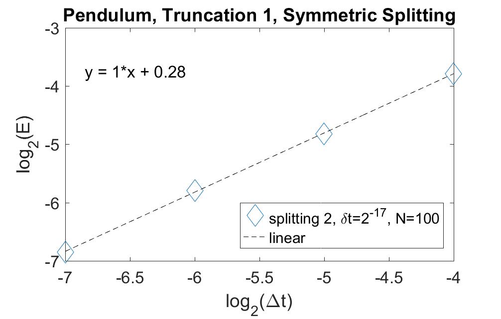
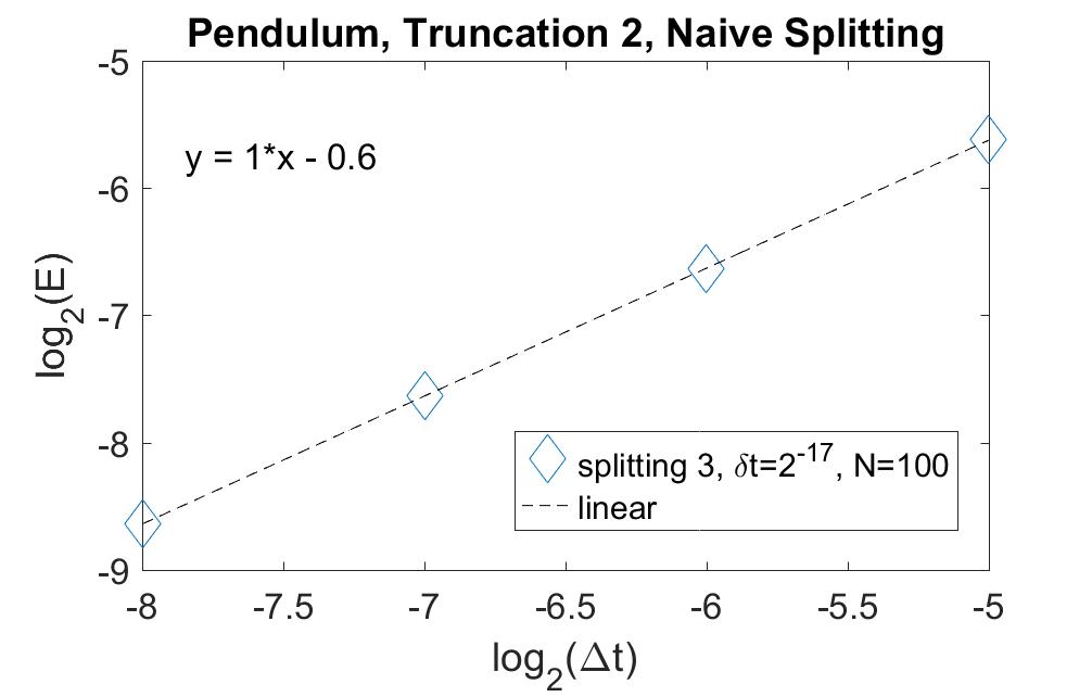
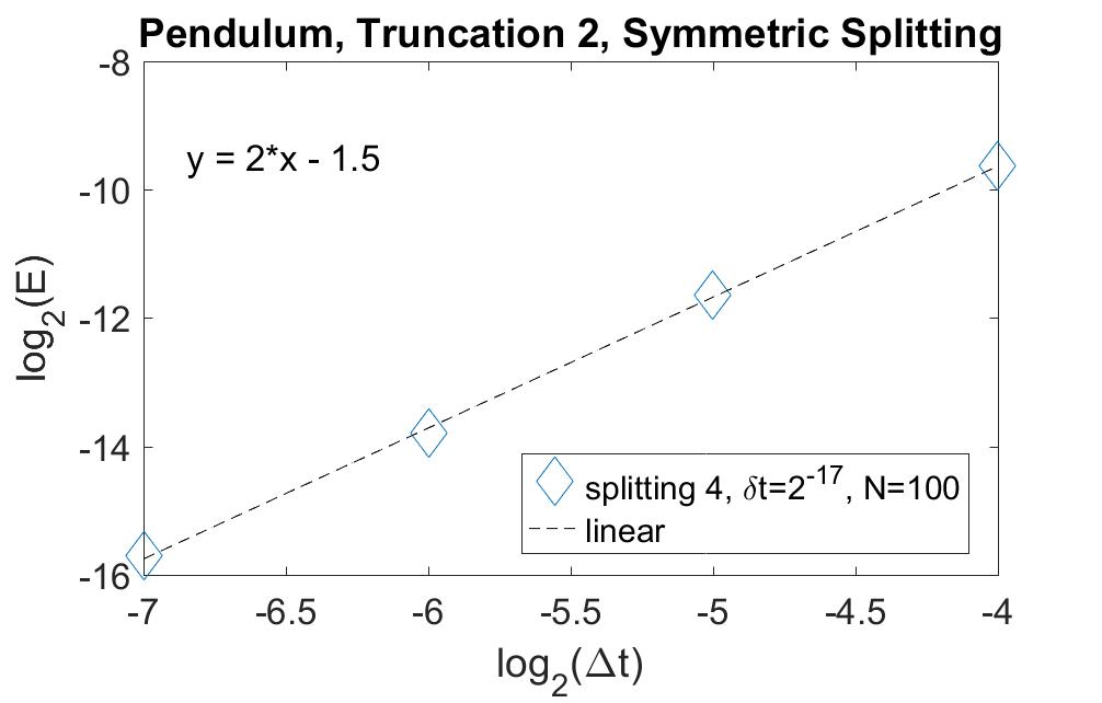
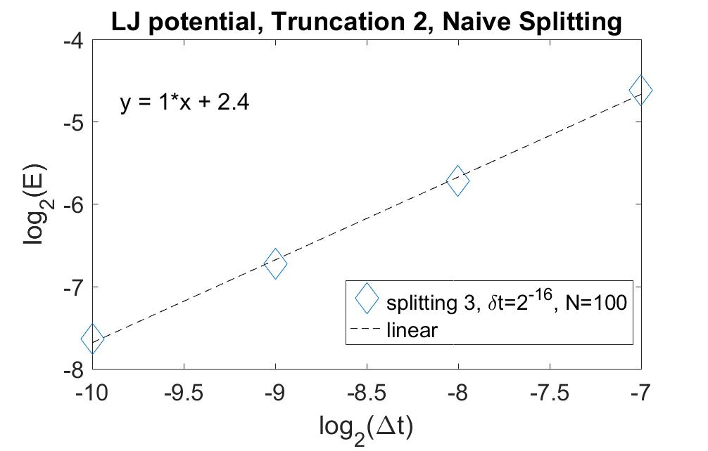
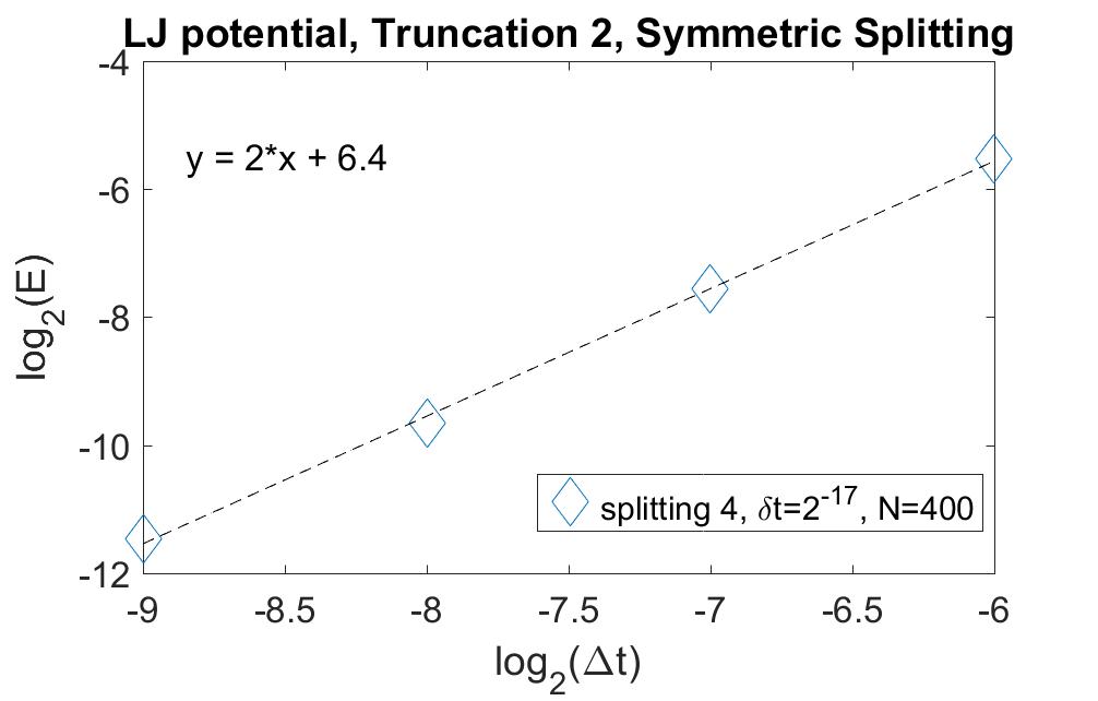
where ξknsubscript𝜉𝑘superscript𝑛\vec{\xi}_{k}\in\mathbb{R}^{n} is a random vector in N(0,In×n)𝑁0subscript𝐼𝑛𝑛N(0,I_{n\times n}) and the increments ξk,ξlsubscript𝜉𝑘subscript𝜉𝑙\vec{\xi}_{k},\vec{\xi}_{l} are independent for kl𝑘𝑙k\neq l. From Fig. 2 and Fig. 3, we see that the (non-symmetric and symmetric) operator splitting methods applied to truncation DΔtIsuperscriptsubscript𝐷Δ𝑡𝐼D_{\Delta t}^{I} both converge with order 1. Therefore, to obtain higher order strong convergence, a further truncation is needed.

4.2 Second-order truncation

Now we consider the truncation of Dtsubscript𝐷𝑡D_{t} which includes the first order bracket [22, eq. 3.22]:

(41) DΔtII=Δt𝒳0+j=1nΔWj𝒳j+12j=1n[Δt,ΔWj][𝒳0,𝒳j].superscriptsubscript𝐷Δ𝑡IIΔ𝑡subscript𝒳0superscriptsubscript𝑗1𝑛Δsuperscript𝑊𝑗subscript𝒳𝑗12superscriptsubscript𝑗1𝑛Δ𝑡Δsuperscript𝑊𝑗subscript𝒳0subscript𝒳𝑗D_{{\Delta t}}^{\rm II}={\Delta t}\mathcal{X}_{0}+\sum_{j=1}^{n}\Delta W^{j}\mathcal{X}_{j}+\frac{1}{2}\sum_{j=1}^{n}[{\Delta t},\Delta W^{j}][\mathcal{X}_{0},\mathcal{X}_{j}].

For the Langevin dynamics model (1), we can write the differential operator [𝒳0,𝒳j]subscript𝒳0subscript𝒳𝑗[\mathcal{X}_{0},\mathcal{X}_{j}] as

(42) [𝒳0,𝒳j]=(12j=1nσj[Δt,ΔWj])x+(12j=1nΓσj[Δt,ΔWj])v,subscript𝒳0subscript𝒳𝑗12superscriptsubscript𝑗1𝑛superscript𝜎𝑗Δ𝑡Δsuperscript𝑊𝑗subscript𝑥12superscriptsubscript𝑗1𝑛Γsuperscript𝜎𝑗Δ𝑡Δsuperscript𝑊𝑗subscript𝑣[\mathcal{X}_{0},\mathcal{X}_{j}]=\left(-\frac{1}{2}\sum_{j=1}^{n}\sigma^{j}[{\Delta t},\Delta W^{j}]\right)\cdot\nabla_{x}+\left(\frac{1}{2}\sum_{j=1}^{n}\Gamma\sigma^{j}[{\Delta t},\Delta W^{j}]\right)\cdot\nabla_{v},

which allows us to rewrite equation (41) above as,

(43) DΔtIIsuperscriptsubscript𝐷Δ𝑡II\displaystyle D_{{\Delta t}}^{\rm II} =(Δtv12j=1nσj[Δt,ΔWj])xabsentΔ𝑡𝑣12superscriptsubscript𝑗1𝑛superscript𝜎𝑗Δ𝑡Δsuperscript𝑊𝑗subscript𝑥\displaystyle=\left({\Delta t}v-\frac{1}{2}\sum_{j=1}^{n}\sigma^{j}[{\Delta t},\Delta W^{j}]\right)\cdot\nabla_{x}
+(Δt(f(x)Γv)+j=1nσjΔWj+12j=1nΓσj[Δt,ΔWj])v.Δ𝑡𝑓𝑥Γ𝑣superscriptsubscript𝑗1𝑛superscript𝜎𝑗Δsuperscript𝑊𝑗12superscriptsubscript𝑗1𝑛Γsuperscript𝜎𝑗Δ𝑡Δsuperscript𝑊𝑗subscript𝑣\displaystyle+\left({\Delta t}\big{(}f(x)-\Gamma v\big{)}+\sum_{j=1}^{n}\sigma^{j}\Delta W^{j}+\frac{1}{2}\sum_{j=1}^{n}\Gamma\sigma^{j}[{\Delta t},\Delta W^{j}]\right)\cdot\nabla_{v}.

This will be referred to as truncation II.

We note in passing that the expression (42) for [𝒳0,𝒳j]subscript𝒳0subscript𝒳𝑗[\mathcal{X}_{0},\mathcal{X}_{j}] is valid so long as the operator is applied to functions that are linear in v𝑣v, which will always be the case in this paper. And for functions linear in v𝑣v, we note that 𝒳0,𝒳jsubscript𝒳0subscript𝒳𝑗\mathcal{X}_{0},\mathcal{X}_{j} equal the differential operators L0,Ljsuperscript𝐿0superscript𝐿𝑗L^{0},L^{j} respectively, which appear in the definition of Itô-Taylor expansions (see [11, Sec. 5.1]).

Now we define Gaussian random variables ΔU=(ΔU1,,ΔUn)Δ𝑈Δsuperscript𝑈1Δsuperscript𝑈𝑛\Delta U=(\Delta U^{1},\dots,\Delta U^{n}), where

(44) ΔUj:=12[Δt,ΔWj]=I(0,j)12ΔtΔWj, j=1,2,,n.formulae-sequenceassignΔsuperscript𝑈𝑗12Δ𝑡Δsuperscript𝑊𝑗subscript𝐼0𝑗12Δ𝑡Δsuperscript𝑊𝑗 𝑗12𝑛\Delta U^{j}:=\frac{1}{2}[{\Delta t},\Delta W^{j}]=I_{(0,j)}-\frac{1}{2}{\Delta t}\Delta W^{j},\text{\quad}j=1,2,\cdots,n.

The random variable ΔUjΔsuperscript𝑈𝑗\Delta U^{j} will play an important role in obtaining higher order strong convergence. For discretizations which lack higher order stochastic integrals (such as I(0,j)subscript𝐼0𝑗I_{(0,j)} in the definition of ΔUjΔsuperscript𝑈𝑗\Delta U^{j}), and only have the increments ΔWjΔsuperscript𝑊𝑗\Delta W^{j}, there is a barrier to higher order convergence. The Euler-Maruyama method obtains the highest convergence rate possible for such schemes, and this barrier is discussed in more detail in the paper by [26, Thm. 3]. As we saw in the Itô-Taylor schemes (7), the higher order schemes require higher order stochastic integrals.

With ΔW:=(ΔW1,,ΔWn)assignΔ𝑊Δsuperscript𝑊1Δsuperscript𝑊𝑛\Delta W:=(\Delta W^{1},\dots,\Delta W^{n}), we have

(45) DΔtII=(ΔtvσΔU)x+(Δt(f(x)Γv)+σΔW+ΓσΔU)vsuperscriptsubscript𝐷Δ𝑡IIΔ𝑡𝑣𝜎Δ𝑈subscript𝑥Δ𝑡𝑓𝑥Γ𝑣𝜎Δ𝑊Γ𝜎Δ𝑈subscript𝑣D_{{\Delta t}}^{\rm II}=\left({\Delta t}v-\sigma\Delta U\right)\cdot\nabla_{x}+\left({\Delta t}(f(x)-\Gamma v)+\sigma\Delta W+\Gamma\sigma\Delta U\right)\cdot\nabla_{v}

Once ΔWΔ𝑊\Delta W and ΔUΔ𝑈\Delta U are realized, the solution corresponds to that of the following ODEs at time t=1𝑡1t=1,

{x=vΔtσΔU,v=f(x)ΔtΓvΔt+σΔW+ΓσΔU.casessuperscript𝑥absent𝑣Δ𝑡𝜎Δ𝑈superscript𝑣absent𝑓𝑥Δ𝑡Γ𝑣Δ𝑡𝜎Δ𝑊Γ𝜎Δ𝑈\begin{cases}x^{\prime}&=v{\Delta t}-\sigma\Delta U,\\ v^{\prime}&=f(x){\Delta t}-\Gamma v{\Delta t}+{\sigma\Delta W}+\Gamma\sigma\Delta U.\end{cases}

A direct expansion of the solutions of the ODEs is given by,

(46) expDII(xkvk)superscript𝐷IImatrixsubscript𝑥𝑘subscript𝑣𝑘\displaystyle\exp D^{\rm II}\left(\begin{matrix}x_{k}\\ v_{k}\end{matrix}\right) =(xkvk)+(vkf(xk)Γvk)Δt+j=1n(0n×1σj)ΔWkjabsentmatrixsubscript𝑥𝑘subscript𝑣𝑘matrixsubscript𝑣𝑘𝑓subscript𝑥𝑘Γsubscript𝑣𝑘Δ𝑡superscriptsubscript𝑗1𝑛matrixsubscript0𝑛1superscript𝜎𝑗Δsuperscriptsubscript𝑊𝑘𝑗\displaystyle=\left(\begin{matrix}x_{k}\\ v_{k}\end{matrix}\right)+\left(\begin{matrix}v_{k}\\ f(x_{k})-\Gamma v_{k}\end{matrix}\right){\Delta t}+\sum_{j=1}^{n}\left(\begin{matrix}0_{n\times 1}\\ \sigma^{j}\end{matrix}\right)\Delta W_{k}^{j}
+(f(xk)Γvkxf(xk)vkΓf(xk)+Γ2vk)Δt22+j=1n(σjΓσj)I(j,0),kmatrix𝑓subscript𝑥𝑘Γsubscript𝑣𝑘subscript𝑥𝑓subscript𝑥𝑘subscript𝑣𝑘Γ𝑓subscript𝑥𝑘superscriptΓ2subscript𝑣𝑘Δsuperscript𝑡22superscriptsubscript𝑗1𝑛matrixsuperscript𝜎𝑗Γsuperscript𝜎𝑗subscript𝐼𝑗0𝑘\displaystyle+\left(\begin{matrix}f(x_{k})-\Gamma v_{k}\\ \nabla_{x}f(x_{k})v_{k}-\Gamma f(x_{k})+\Gamma^{2}v_{k}\end{matrix}\right)\frac{{\Delta t}^{2}}{2}+\sum_{j=1}^{n}\left(\begin{matrix}\sigma^{j}\\ -\Gamma\sigma^{j}\end{matrix}\right)I_{(j,0),k}
+j=1n(Γσjxf(xk)σjΓ2σj)ΔtΔUkj2+H.O.T.,superscriptsubscript𝑗1𝑛matrixΓsuperscript𝜎𝑗subscript𝑥𝑓subscript𝑥𝑘superscript𝜎𝑗superscriptΓ2superscript𝜎𝑗Δ𝑡Δsuperscriptsubscript𝑈𝑘𝑗2H.O.T.\displaystyle+\sum_{j=1}^{n}\left(\begin{matrix}\Gamma\sigma^{j}\\ -\nabla_{x}f(x_{k})\sigma^{j}-\Gamma^{2}\sigma^{j}\end{matrix}\right)\frac{{\Delta t}\Delta U_{k}^{j}}{2}+\text{H.O.T.},

where H.O.T. stands for Higher Order Terms. We observe that the stochastic integrals I(0,j)subscript𝐼0𝑗I_{(0,j)} do not appear among the lower order terms. This is because the commutator [Δt,ΔWj](=2ΔUj)annotatedΔ𝑡Δsuperscript𝑊𝑗absent2Δsuperscript𝑈𝑗[{\Delta t},\Delta W^{j}](=2\Delta U^{j}) in DIIsuperscript𝐷IID^{\rm II} allows us to include the stochastic integrals I(j,0)subscript𝐼𝑗0I_{(j,0)} that we see in the higher order Itô-Taylor expansions, while simultaneously excluding the unnecessary integrals I(0,j)subscript𝐼0𝑗I_{(0,j)}. A short derivation of the expansion above can be seen in Section 5.4.

Thus we have,

Theorem 3.

The operator exp(DΔtII)superscriptsubscript𝐷Δ𝑡II\exp\left(D_{{\Delta t}}^{\rm II}\right) generates a solution with strong order 2.

For the numerical implementation, we use the following splitting, DΔtII=A+Bsuperscriptsubscript𝐷Δ𝑡II𝐴𝐵D_{{\Delta t}}^{\rm II}=A+B, where,

(47) A=𝐴absent\displaystyle A= (ΔtvσΔU)xΔ𝑡𝑣𝜎Δ𝑈subscript𝑥\displaystyle\big{(}{\Delta t}v-\sigma\Delta U\big{)}\cdot\nabla_{x}
B=𝐵absent\displaystyle B= (f(x)ΔtΓvΔt+σΔW+σΓΔU)v.𝑓𝑥Δ𝑡Γ𝑣Δ𝑡𝜎Δ𝑊𝜎ΓΔ𝑈subscript𝑣\displaystyle\big{(}f(x){\Delta t}-\Gamma v{\Delta t}+{\sigma\Delta W}+\sigma\Gamma\Delta U\big{)}\cdot\nabla_{v}.

For practical implementations, we denote the increments by ΔWkΔsubscript𝑊𝑘\Delta W_{k} and ΔUkΔsubscript𝑈𝑘\Delta U_{k} at the k𝑘kth step (k=0,1,,nT1𝑘01subscript𝑛𝑇1k=0,1,\dots,n_{T}-1), and sample them using the covariance matrix:

(48) C=def(𝔼(ΔWk2)𝔼(ΔWkΔUk)𝔼(ΔUkΔWk)𝔼(ΔUk2))=(ΔtIn×n0n×n0n×nΔt312In×n).𝐶defmatrix𝔼Δsuperscriptsubscript𝑊𝑘2𝔼Δsubscript𝑊𝑘Δsubscript𝑈𝑘𝔼Δsubscript𝑈𝑘Δsubscript𝑊𝑘𝔼Δsuperscriptsubscript𝑈𝑘2matrixΔ𝑡subscript𝐼𝑛𝑛subscript0𝑛𝑛subscript0𝑛𝑛Δsuperscript𝑡312subscript𝐼𝑛𝑛C\overset{\text{def}}{=}\left(\begin{matrix}\mathbb{E}(\Delta W_{k}^{2})&\mathbb{E}(\Delta W_{k}\Delta U_{k})\\ \mathbb{E}(\Delta U_{k}\Delta W_{k})&\mathbb{E}(\Delta U_{k}^{2})\\ \end{matrix}\right)=\left(\begin{matrix}{\Delta t}I_{n\times n}&0_{n\times n}\\ 0_{n\times n}&\frac{{\Delta t}^{3}}{12}I_{n\times n}\\ \end{matrix}\right).

This covariance formula can be verified using [11, p. 223] and [31, Sec. 6.12]. We note that the right hand side of the formula does not depend on k𝑘k, and so the sampling statistics are the same at each step. Each of the ODEs corresponding to these operators has explicit solutions. Using the BCH formula, and a comparison with the Itô-Taylor expansion, we found that,

Theorem 4.

The non-symmetric splitting scheme

exp(DΔtII)exp(A)exp(B)superscriptsubscript𝐷Δ𝑡II𝐴𝐵\exp(D_{{\Delta t}}^{\rm{\rm II}})\approx\exp(A)\exp(B)

yields an approximation with strong order 1. The symmetric splitting scheme,

exp(DΔtII)exp(A2)exp(B)exp(A2)superscriptsubscript𝐷Δ𝑡II𝐴2𝐵𝐴2\exp(D_{{\Delta t}}^{\rm{\rm II}})\approx\exp(\frac{A}{2})\exp(B)\exp(\frac{A}{2})

gives strong order 2, and the other symmetric splitting scheme,

exp(B2)exp(A)exp(B2)𝐵2𝐴𝐵2\exp(\frac{B}{2})\exp(A)\exp(\frac{B}{2})

has the same order [7].

Proof 4.2.

For the symmetric-splitting, the proof is identical to the proof of Theorem 2, using the triangle inequality, the fact that expDΔtIIsuperscriptsubscript𝐷Δ𝑡II\exp D_{{\Delta t}}^{\rm II} generates a strong order 2 solution, and the well-known fact that the symmetric splitting for ODEs has order 2 (see [7]).

For the non-symmetric splitting, a direct Taylor expansion shows that the low order convergence of the splitting reduces the overall convergence to 1. The expansion is straightforward and left to the interested reader.

The non-symmetric splitting, Algorithm 1, involves two steps, where c0=eΓΔtsubscript𝑐0superscript𝑒ΓΔ𝑡c_{0}=e^{-\Gamma{\Delta t}} and c1=Γ1(Ic0)subscript𝑐1superscriptΓ1𝐼subscript𝑐0c_{1}=\Gamma^{-1}(I-c_{0}).

Algorithm 1 Non-symmetric splitting of truncation II
  Given x=x0,v=v0formulae-sequence𝑥subscript𝑥0𝑣subscript𝑣0x=x_{0},v=v_{0}, evaluate f(x)𝑓𝑥f(x)
  for k=0,1,,nT1𝑘01subscript𝑛𝑇1k=0,1,\dots,n_{T}-1 do
     Sample ΔWΔ𝑊\Delta W and ΔUΔ𝑈\Delta U according to (48)
     Update vc0v+c1Δt(f(x)Δt+σΔWk+ΓσΔU)𝑣subscript𝑐0𝑣subscript𝑐1Δ𝑡𝑓𝑥Δ𝑡𝜎Δsubscript𝑊𝑘Γ𝜎Δ𝑈v\longleftarrow c_{0}v+\frac{c_{1}}{{\Delta t}}\left(f(x){\Delta t}+\sigma\Delta W_{k}+\Gamma\sigma\Delta U\right)
     Update xx+ΔtvσΔU𝑥𝑥Δ𝑡𝑣𝜎Δ𝑈x\longleftarrow x+{\Delta t}v-\sigma\Delta U
     Evaluate f(x)𝑓𝑥f(x)
  end for
  return  x=x(T),v=v(T)formulae-sequence𝑥𝑥𝑇𝑣𝑣𝑇x=x(T),v=v(T)

The symmetric splitting, Algorithm 2, involves three steps.

Algorithm 2 Symmetric splitting of truncation II
  Given x=x0,v=v0formulae-sequence𝑥subscript𝑥0𝑣subscript𝑣0x=x_{0},v=v_{0}, evaluate f(x)𝑓𝑥f(x)
  for k=0,1,,nT1𝑘01subscript𝑛𝑇1k=0,1,\dots,n_{T}-1 do
     Sample ΔWΔ𝑊\Delta W and ΔUΔ𝑈\Delta U according to (48)
     Update xx+Δt2(vσΔUΔt)𝑥𝑥Δ𝑡2𝑣𝜎Δ𝑈Δ𝑡x\longleftarrow x+\frac{{\Delta t}}{2}\left(v-\frac{\sigma\Delta U}{{\Delta t}}\right)
     Update vc0v+c1Δt(f(x)Δt+σΔW+ΓσΔU)𝑣subscript𝑐0𝑣subscript𝑐1Δ𝑡𝑓𝑥Δ𝑡𝜎Δ𝑊Γ𝜎Δ𝑈v\longleftarrow c_{0}v+\frac{c_{1}}{{\Delta t}}\left(f(x){\Delta t}+\sigma\Delta W+\Gamma\sigma\Delta U\right)
     Update xx+Δt2(vσΔUΔt)𝑥𝑥Δ𝑡2𝑣𝜎Δ𝑈Δ𝑡x\longleftarrow x+\frac{{\Delta t}}{2}\left(v-\frac{\sigma\Delta U}{{\Delta t}}\right)
     Evaluate f(x)𝑓𝑥f(x)
  end for
  return  x=x(T),v=v(T)formulae-sequence𝑥𝑥𝑇𝑣𝑣𝑇x=x(T),v=v(T)

The numerical tests in Fig. 2 and Fig. 3 confirmed the convergence orders for truncation II with the naive and symmetric splittings methods can be found in Section 6. The symmetric splitting method has the same strong convergence order as the SVV method. It is slightly easier to implement.

4.3 Under-damped (Γ0Γ0\Gamma\rightarrow 0) and over-damped (Γ1much-greater-thanΓ1\Gamma{\color[rgb]{0,0,0}\gg}1) cases

We consider the 2nd order symmetric splitting method above, given by the algorithm Algorithm 2, in the under-damped situation, Γ0+Γsuperscript0\Gamma\rightarrow 0^{+}. Assuming the fluctuation dissipation theorem (2) holds, σ0+𝜎superscript0\sigma\rightarrow 0^{+} as Γ0+Γsuperscript0\Gamma\rightarrow 0^{+}. Then the constant matrices c0,c1subscript𝑐0subscript𝑐1c_{0},c_{1} in the equations Algorithm 2 become, in the limit,

(49) limΓ0+c0subscriptΓsuperscript0subscript𝑐0\displaystyle\lim_{\Gamma\rightarrow 0^{+}}c_{0} =limΓ0+eΓΔt=IabsentsubscriptΓsuperscript0superscript𝑒ΓΔ𝑡𝐼\displaystyle=\lim_{\Gamma\rightarrow 0^{+}}e^{-\Gamma{\Delta t}}=I
(50) limΓ0+c1subscriptΓsuperscript0subscript𝑐1\displaystyle\lim_{\Gamma\rightarrow 0^{+}}c_{1} =limΓ0+Γ1(Ic0)=limΓ0+ΔteΓΔt=ΔtI,absentsubscriptΓsuperscript0superscriptΓ1𝐼subscript𝑐0subscriptΓsuperscript0Δ𝑡superscript𝑒ΓΔ𝑡Δ𝑡𝐼\displaystyle=\lim_{\Gamma\rightarrow 0^{+}}\Gamma^{-1}(I-c_{0})=\lim_{\Gamma\rightarrow 0^{+}}{\Delta t}e^{-\Gamma{\Delta t}}={\Delta t}{\color[rgb]{0,0,0}I},

where the second limit-equality holds due to l’Hôpital’s rule. As a result, the equations in Algorithm 2 become,

(51) xn+1/2subscript𝑥𝑛12\displaystyle x_{n+1/2} =xn+Δtvn2absentsubscript𝑥𝑛Δ𝑡subscript𝑣𝑛2\displaystyle=x_{n}+\frac{{\Delta t}v_{n}}{2}
(52) vn+1subscript𝑣𝑛1\displaystyle v_{n+1} =vn+Δtf(xn+1/2)absentsubscript𝑣𝑛Δ𝑡𝑓subscript𝑥𝑛12\displaystyle=v_{n}+{\Delta t}f(x_{n+1/2})
(53) xn+1subscript𝑥𝑛1\displaystyle x_{n+1} =xn+1/2+Δtvn+12,absentsubscript𝑥𝑛12Δ𝑡subscript𝑣𝑛12\displaystyle=x_{n+1/2}+\frac{{\Delta t}v_{n+1}}{2},

that is, the under-damped limit of the 2nd order operator splitting method is the velocity Verlet method for the corresponding deterministic Hamiltonian dynamics [16],

(54) x¨=f(x).¨𝑥𝑓𝑥\ddot{x}=f(x).

Next, we turn to the over-damped limit, Γ1much-greater-thanΓ1\Gamma\gg 1 large, for truncation IIII\rm II with the non-symmetric splitting. If we take Γ1much-greater-thanΓ1\Gamma\gg 1 large, the term c00subscript𝑐00c_{0}\approx 0 is negligible and c1Γ1subscript𝑐1superscriptΓ1c_{1}\approx\Gamma^{-1}, so that the steps become independent of v𝑣v:

(55) vk+1subscript𝑣𝑘1\displaystyle v_{k+1} =Γ1f(xk)+Γ1σΔWkΔt+σΔUkΔtabsentsuperscriptΓ1𝑓subscript𝑥𝑘superscriptΓ1𝜎Δsubscript𝑊𝑘Δ𝑡𝜎Δsubscript𝑈𝑘Δ𝑡\displaystyle=\Gamma^{-1}f(x_{k})+\frac{\Gamma^{-1}\sigma\Delta W_{k}}{{\Delta t}}+\frac{\sigma\Delta U_{k}}{{\Delta t}}
xk+1subscript𝑥𝑘1\displaystyle x_{k+1} =xk+Δt(Γ1f(xk)+Γ1σΔWkΔt+σΔUkΔt)σΔUkabsentsubscript𝑥𝑘Δ𝑡superscriptΓ1𝑓subscript𝑥𝑘superscriptΓ1𝜎Δsubscript𝑊𝑘Δ𝑡𝜎Δsubscript𝑈𝑘Δ𝑡𝜎Δsubscript𝑈𝑘\displaystyle=x_{k}+{\Delta t}\left(\Gamma^{-1}f(x_{k})+\frac{\Gamma^{-1}\sigma\Delta W_{k}}{{\Delta t}}+\frac{\sigma\Delta U_{k}}{{\Delta t}}\right)-\sigma\Delta U_{k}
=xk+ΔtΓ1f(xk)+Γ1σΔWk.absentsubscript𝑥𝑘Δ𝑡superscriptΓ1𝑓subscript𝑥𝑘superscriptΓ1𝜎Δsubscript𝑊𝑘\displaystyle=x_{k}+{\Delta t}\Gamma^{-1}f(x_{k})+\Gamma^{-1}\sigma\Delta W_{k}.

In particular, the second step is the Euler-Maruyama method for the position- only first degree SDE,

(56) dx=Γ1f(x)dt+Γ1σdWt.𝑑𝑥superscriptΓ1𝑓𝑥𝑑𝑡superscriptΓ1𝜎𝑑subscript𝑊𝑡dx=\Gamma^{-1}f(x)dt+\Gamma^{-1}\sigma dW_{t}.

Thus the over-damped limit of the non-symmetric splitting with truncation IIII\rm II is the Euler-Maruyama method for the first degree SDE above.

Turning to the symmetric splitting in the over-damped limit, we consider the splitting

(57) exp(B/2)exp(A)exp(B/2).𝐵2𝐴𝐵2\exp(B/2)\exp(A)\exp(B/2).

In this setting, the first two steps give us the Euler-Maruyama method for the reduced first order SDE (56). Indeed, we have

(58) vk+1/2subscript𝑣𝑘12\displaystyle v_{k+1/2} =Γ1f(xk)+Γ1σΔWkΔt+σΔUkΔtabsentsuperscriptΓ1𝑓subscript𝑥𝑘superscriptΓ1𝜎Δsubscript𝑊𝑘Δ𝑡𝜎Δsubscript𝑈𝑘Δ𝑡\displaystyle=\Gamma^{-1}f(x_{k})+\frac{\Gamma^{-1}\sigma\Delta W_{k}}{{\Delta t}}+\frac{\sigma\Delta U_{k}}{{\Delta t}}
xk+1subscript𝑥𝑘1\displaystyle x_{k+1} =xk+vk+1/2ΔtσΔUkabsentsubscript𝑥𝑘subscript𝑣𝑘12Δ𝑡𝜎Δsubscript𝑈𝑘\displaystyle=x_{k}+v_{k+1/2}{\Delta t}-\sigma\Delta U_{k}
=xk+Δt(Γ1f(xk)+Γ1σΔWkΔt+σΔUkΔt)σΔUkabsentsubscript𝑥𝑘Δ𝑡superscriptΓ1𝑓subscript𝑥𝑘superscriptΓ1𝜎Δsubscript𝑊𝑘Δ𝑡𝜎Δsubscript𝑈𝑘Δ𝑡𝜎Δsubscript𝑈𝑘\displaystyle=x_{k}+{\Delta t}\left(\Gamma^{-1}f(x_{k})+\frac{\Gamma^{-1}\sigma\Delta W_{k}}{{\Delta t}}+\frac{\sigma\Delta U_{k}}{{\Delta t}}\right)-\sigma\Delta U_{k}
=xk+Γ1f(xk)Δt+Γ1σΔWk,absentsubscript𝑥𝑘superscriptΓ1𝑓subscript𝑥𝑘Δ𝑡superscriptΓ1𝜎Δsubscript𝑊𝑘\displaystyle=x_{k}+\Gamma^{-1}f(x_{k}){\Delta t}+\Gamma^{-1}\sigma\Delta W_{k},

and the last equation, xk+1=xk+Γ1f(xk)Δt+Γ1σΔWk,subscript𝑥𝑘1subscript𝑥𝑘superscriptΓ1𝑓subscript𝑥𝑘Δ𝑡superscriptΓ1𝜎Δsubscript𝑊𝑘x_{k+1}=x_{k}+\Gamma^{-1}f(x_{k}){\Delta t}+\Gamma^{-1}\sigma\Delta W_{k}, which is independent of v𝑣v, is precisely the Euler-Maruyama method for dxt=Γ1f(xt)dt+Γ1σdWt.𝑑subscript𝑥𝑡superscriptΓ1𝑓subscript𝑥𝑡𝑑𝑡superscriptΓ1𝜎𝑑subscript𝑊𝑡dx_{t}=\Gamma^{-1}f(x_{t})dt+\Gamma^{-1}\sigma dW_{t}.

4.4 Third-order truncation

Finally, we turn to the next truncation,

(59) DΔtIII=Δt+j=1nΔWj𝒳j+j=1nΔUj[𝒳0,𝒳j]+j=1nΔVj[[𝒳0,𝒳j],𝒳0]superscriptsubscript𝐷Δ𝑡IIIΔ𝑡superscriptsubscript𝑗1𝑛Δsuperscript𝑊𝑗subscript𝒳𝑗superscriptsubscript𝑗1𝑛Δsuperscript𝑈𝑗subscript𝒳0subscript𝒳𝑗superscriptsubscript𝑗1𝑛Δsuperscript𝑉𝑗subscript𝒳0subscript𝒳𝑗subscript𝒳0D_{{\Delta t}}^{\rm III}={\Delta t}+\sum_{j=1}^{n}\Delta W^{j}\mathcal{X}_{j}+\sum_{j=1}^{n}\Delta U^{j}[\mathcal{X}_{0},\mathcal{X}_{j}]+\sum_{j=1}^{n}\Delta V^{j}\left[[\mathcal{X}_{0},\mathcal{X}_{j}],\mathcal{X}_{0}\right]

where

(60) ΔVjΔsuperscript𝑉𝑗\displaystyle\Delta V^{j} =[[Δt,ΔWj],Δt]=118(2I(0,j,0)2I(j,0,0)+ΔtI(j,0)ΔtI(0,j))absentΔ𝑡Δsuperscript𝑊𝑗Δ𝑡1182subscript𝐼0𝑗02subscript𝐼𝑗00Δ𝑡subscript𝐼𝑗0Δ𝑡subscript𝐼0𝑗\displaystyle=\left[[{\Delta t},\Delta W^{j}],{\Delta t}\right]=\frac{1}{18}\left(2I_{(0,j,0)}-2I_{(j,0,0)}+{\Delta t}I_{(j,0)}-{\Delta t}I_{(0,j)}\right)
=19(I(0,j,0)I(j,0,0)ΔtΔUj)absent19subscript𝐼0𝑗0subscript𝐼𝑗00Δ𝑡Δsuperscript𝑈𝑗\displaystyle=\frac{1}{9}\left(I_{(0,j,0)}-I_{(j,0,0)}-{\Delta t}\Delta U^{j}\right)

and ΔV=(ΔV1,,ΔVn)Δ𝑉Δsuperscript𝑉1Δsuperscript𝑉𝑛\Delta V=(\Delta V^{1},\dots,\Delta V^{n}). This comes from [22, eq. 2.15], using the fact that [[𝒳0,𝒳i],𝒳j]=0subscript𝒳0subscript𝒳𝑖subscript𝒳𝑗0[[\mathcal{X}_{0},\mathcal{X}_{i}],\mathcal{X}_{j}]=0 when i,j0𝑖𝑗0i,j\neq 0 for additive noise. Since we have the following expressions for all relevant brackets,

(61) 𝒳0subscript𝒳0\displaystyle\mathcal{X}_{0} =vx+(f(x)Γv)vabsent𝑣subscript𝑥𝑓𝑥Γ𝑣subscript𝑣\displaystyle=v\cdot\nabla_{x}+(f(x)-\Gamma v)\cdot\nabla_{v}
𝒳jsubscript𝒳𝑗\displaystyle\mathcal{X}_{j} =σjvabsentsuperscript𝜎𝑗subscript𝑣\displaystyle=\sigma^{j}\cdot\nabla_{v}
[𝒳0,𝒳j]subscript𝒳0subscript𝒳𝑗\displaystyle\left[\mathcal{X}_{0},\mathcal{X}_{j}\right] =σjx+Γσjvabsentsuperscript𝜎𝑗subscript𝑥Γsuperscript𝜎𝑗subscript𝑣\displaystyle=-\sigma^{j}\cdot\nabla_{x}+\Gamma\sigma^{j}\cdot\nabla_{v}
[[𝒳0,𝒳j],𝒳0]subscript𝒳0subscript𝒳𝑗subscript𝒳0\displaystyle\left[[\mathcal{X}_{0},\mathcal{X}_{j}],\mathcal{X}_{0}\right] =Γσjx(Df(x)σj+Γ2σj)v,absentΓsuperscript𝜎𝑗subscript𝑥𝐷𝑓𝑥superscript𝜎𝑗superscriptΓ2superscript𝜎𝑗subscript𝑣\displaystyle=\Gamma\sigma^{j}\cdot\nabla_{x}-(Df(x)\sigma^{j}+\Gamma^{2}\sigma^{j})\cdot\nabla_{v},

we can rewrite DΔtIIIsuperscriptsubscript𝐷Δ𝑡IIID_{{\Delta t}}^{\rm III} in (59) as

(62) DΔtIIIsuperscriptsubscript𝐷Δ𝑡III\displaystyle D_{{\Delta t}}^{\rm III} =(vΔtσΔU+ΓσΔV)xabsent𝑣Δ𝑡𝜎Δ𝑈Γ𝜎Δ𝑉subscript𝑥\displaystyle=\left(v{\Delta t}-\sigma\Delta U+\Gamma\sigma\Delta V\right)\cdot\nabla_{x}
+((f(x)Γv)Δt+σΔW+ΓσΔU(Df(x)σ+Γ2σ)ΔV)v,𝑓𝑥Γ𝑣Δ𝑡𝜎Δ𝑊Γ𝜎Δ𝑈𝐷𝑓𝑥𝜎superscriptΓ2𝜎Δ𝑉subscript𝑣\displaystyle+\left((f(x)-\Gamma v){\Delta t}+\sigma\Delta W+\Gamma\sigma\Delta U-(Df(x)\sigma+\Gamma^{2}\sigma)\Delta V\right)\cdot\nabla_{v},

which gives us the ODEs

(63) {x=vΔtσΔU+ΓσΔVv=(f(x)Γv)Δt+σΔW+ΓσΔU(Df(x)σ+Γ2σ)ΔV.casessuperscript𝑥absent𝑣Δ𝑡𝜎Δ𝑈Γ𝜎Δ𝑉superscript𝑣absent𝑓𝑥Γ𝑣Δ𝑡𝜎Δ𝑊Γ𝜎Δ𝑈𝐷𝑓𝑥𝜎superscriptΓ2𝜎Δ𝑉\displaystyle\begin{cases}x^{\prime}&=v{\Delta t}-\sigma\Delta U+\Gamma\sigma\Delta V\\ v^{\prime}&=(f(x)-\Gamma v){\Delta t}+\sigma\Delta W+\Gamma\sigma\Delta U-(Df(x)\sigma+\Gamma^{2}\sigma)\Delta V.\end{cases}

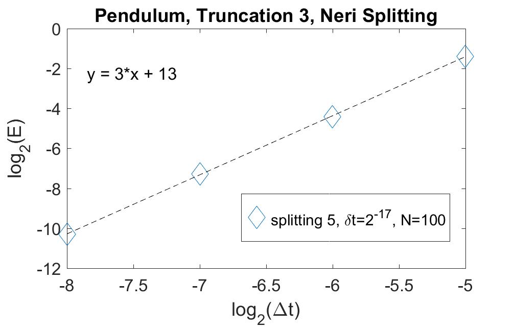
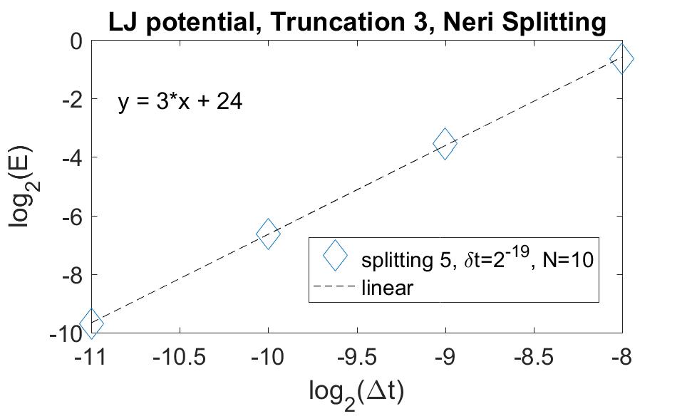
We do not have a complete proof that expDΔtIIIsuperscriptsubscript𝐷Δ𝑡III\exp D_{{\Delta t}}^{\rm III} generates solutions with strong order 3. Although we have the intuition that this can be proven in a similar way to the way we proved the convergence orders of the solutions generated by expDΔtIsuperscriptsubscript𝐷Δ𝑡I\exp D_{{\Delta t}}^{\rm I} and expDΔtIIsuperscriptsubscript𝐷Δ𝑡II\exp D_{{\Delta t}}^{\rm II}, but the calculations will be more complicated. The numerical evidence supports this conjecture, see Fig. 2 and Fig. 3.

For the numerical implementation, we use the splitting DΔtIII=A+Bsuperscriptsubscript𝐷Δ𝑡III𝐴𝐵D_{{\Delta t}}^{\rm III}=A+B where,

(64) A𝐴\displaystyle A =(vΔtσΔU+ΓσΔV)xabsent𝑣Δ𝑡𝜎Δ𝑈Γ𝜎Δ𝑉subscript𝑥\displaystyle=\left(v{\Delta t}-\sigma\Delta U+\Gamma\sigma\Delta V\right)\cdot\nabla_{x}
B𝐵\displaystyle B =((f(x)Γv)Δt+σΔW+ΓσΔU(Df(x)σ+Γ2σ)ΔV)v,absent𝑓𝑥Γ𝑣Δ𝑡𝜎Δ𝑊Γ𝜎Δ𝑈𝐷𝑓𝑥𝜎superscriptΓ2𝜎Δ𝑉subscript𝑣\displaystyle=\left((f(x)-\Gamma v){\Delta t}+\sigma\Delta W+\Gamma\sigma\Delta U-(Df(x)\sigma+\Gamma^{2}\sigma)\Delta V\right)\cdot\nabla_{v},

and the two corresponding ODEs are given by

(65) {x=vΔtσΔU+ΓσΔVv=0casessuperscript𝑥absent𝑣Δ𝑡𝜎Δ𝑈Γ𝜎Δ𝑉superscript𝑣absent0\displaystyle\begin{cases}x^{\prime}&=v{\Delta t}-\sigma\Delta U+\Gamma\sigma\Delta V\\ v^{\prime}&=0\end{cases}

and

(66) {x=0v=(f(x)Γv)Δt+σΔW+ΓσΔU(Df(x)σ+Γ2σ)ΔV.casessuperscript𝑥absent0superscript𝑣absent𝑓𝑥Γ𝑣Δ𝑡𝜎Δ𝑊Γ𝜎Δ𝑈𝐷𝑓𝑥𝜎superscriptΓ2𝜎Δ𝑉\displaystyle\begin{cases}x^{\prime}&=0\\ v^{\prime}&=(f(x)-\Gamma v){\Delta t}+\sigma\Delta W+\Gamma\sigma\Delta U-(Df(x)\sigma+\Gamma^{2}\sigma)\Delta V.\end{cases}

They have explicit solutions , at time tk+1=(k+1)Δtsubscript𝑡𝑘1𝑘1Δ𝑡t_{k+1}=(k+1){\Delta t}, given by,

(67) xk+1subscript𝑥𝑘1\displaystyle x_{k+1} =xk+Δt(vkσΔUkΔt+ΓσΔVkΔt)absentsubscript𝑥𝑘Δ𝑡subscript𝑣𝑘𝜎Δsubscript𝑈𝑘Δ𝑡Γ𝜎Δsubscript𝑉𝑘Δ𝑡\displaystyle=x_{k}+{\Delta t}\left(v_{k}-\frac{\sigma\Delta U_{k}}{{\Delta t}}+\frac{\Gamma\sigma\Delta V_{k}}{{\Delta t}}\right)

and

(68) vk+1subscript𝑣𝑘1\displaystyle v_{k+1} =c0vk+c1Δt(f(xk)Δt+σΔWk+ΓσΔUk(xf(xk)σ+Γ2σ)ΔVk)absentsubscript𝑐0subscript𝑣𝑘subscript𝑐1Δ𝑡𝑓subscript𝑥𝑘Δ𝑡𝜎Δsubscript𝑊𝑘Γ𝜎Δsubscript𝑈𝑘subscript𝑥𝑓subscript𝑥𝑘𝜎superscriptΓ2𝜎Δsubscript𝑉𝑘\displaystyle=c_{0}v_{k}+\frac{c_{1}}{{\Delta t}}\left(f(x_{k}){\Delta t}+\sigma\Delta W_{k}+\Gamma\sigma\Delta U_{k}-(\nabla_{x}f(x_{k})\sigma+\Gamma^{2}\sigma)\Delta V_{k}\right)

where again c0=exp(ΓΔt)subscript𝑐0ΓΔ𝑡c_{0}=\exp(-\Gamma{\Delta t}) and c1=Γ1(Ic0)subscript𝑐1superscriptΓ1𝐼subscript𝑐0c_{1}=\Gamma^{-1}(I-c_{0}). If the coefficient xf(xk)σ+Γ2σsubscript𝑥𝑓subscript𝑥𝑘𝜎superscriptΓ2𝜎\nabla_{x}f(x_{k})\sigma+\Gamma^{2}\sigma of ΔVkΔsubscript𝑉𝑘\Delta V_{k} is zero, this method is reduced to truncation II. We acknowledge and highlight that truncation IIIIII\rm III requires computing the derivative of the potential function f𝑓f. However, this is one fewer derivative than is required by the Itô-Taylor approximation, which requires the second order derivatives. (See the last formula in (7).)

In the implementation, the term xf(x)σΔVsubscript𝑥𝑓𝑥𝜎Δ𝑉\nabla_{x}f(x)\sigma{\color[rgb]{0,0,0}\Delta V} will be approximated by a finite-difference formula,

(69) xf(x)σΔVf(x+εσΔV)f(x)ε, 0<ϵ1.formulae-sequencesubscript𝑥𝑓𝑥𝜎Δ𝑉𝑓𝑥𝜀𝜎Δ𝑉𝑓𝑥𝜀 0italic-ϵmuch-less-than1\nabla_{x}f(x)\sigma\Delta V\approx\frac{f(x+\varepsilon\sigma\Delta V)-f(x)}{\varepsilon},\text{\quad}0<\epsilon{\color[rgb]{0,0,0}\ll}1.

In our numerical convergence tests, we took ϵitalic-ϵ\epsilon to be equal to the small step size δt=219𝛿𝑡superscript219\delta{t}=2^{-19} for the discretized Brownian motion, which stays fixed while the larger step size ΔtΔ𝑡\Delta{t} for the discretized solution of the SDE varies.

In principle, the symmetric splitting methods applied to ODEs have order 2. In order to achieve higher order of accuracy, we solve the ODEs (63) using the Neri’s splitting method [36], which consists of alternating the operators in (64) three times:

(70) exp(DIII)superscript𝐷III\displaystyle\exp(D^{\rm III}) exp(a1A)exp(b1B)exp(a2A)exp(b2B)exp(a3A)exp(b3B)exp(a4A),absentsubscript𝑎1𝐴subscript𝑏1𝐵subscript𝑎2𝐴subscript𝑏2𝐵subscript𝑎3𝐴subscript𝑏3𝐵subscript𝑎4𝐴\displaystyle\approx\exp(a_{1}A)\exp(b_{1}B)\exp(a_{2}A)\exp(b_{2}B)\exp(a_{3}A)\exp(b_{3}B)\exp(a_{4}A),
where a1where subscript𝑎1\displaystyle\text{where\quad}a_{1} =12(223), a2=12a1, a3=a2, a4=a1,formulae-sequenceabsent12232formulae-sequence subscript𝑎212subscript𝑎1formulae-sequence subscript𝑎3subscript𝑎2 subscript𝑎4subscript𝑎1\displaystyle=\frac{1}{2(2-\sqrt[3]{2})},\text{\quad}a_{2}=\frac{1}{2}-a_{1},\text{\quad}a_{3}=a_{2},\text{\quad}a_{4}=a_{1},
and b1and subscript𝑏1\displaystyle\text{and\quad}b_{1} =1223, b2=12b1, b3=b1.formulae-sequenceabsent1232formulae-sequence subscript𝑏212subscript𝑏1 subscript𝑏3subscript𝑏1\displaystyle=\frac{1}{2-\sqrt[3]{2}},\text{\quad}b_{2}=1-2b_{1},\text{\quad}b_{3}=b_{1}.

We wish to highlight that to obtain such high order of accuracy at least one of the steps has to be negative, which is well known (see [7, Ch. 3]).


For practical implementations, the joint covariances of ΔWk,ΔUkΔsubscript𝑊𝑘Δsubscript𝑈𝑘\Delta W_{k},\Delta U_{k}, and ΔVkΔsubscript𝑉𝑘\Delta V_{k} are needed in order to sample these mean-zero Gaussian random variables. Using [11, p. 223], it can be shown (see [31, Sec. 6.12]) that

(71) C=def𝐶def\displaystyle C\overset{\text{def}}{=} (𝔼(ΔWk2)𝔼(ΔWkΔUk)𝔼(ΔWkΔVk)𝔼(ΔUkΔWk)𝔼(ΔUk2)𝔼(ΔUkΔVk)𝔼(ΔVkΔWk)𝔼(ΔVkΔUk)𝔼(ΔVk2))matrix𝔼Δsuperscriptsubscript𝑊𝑘2𝔼Δsubscript𝑊𝑘Δsubscript𝑈𝑘𝔼Δsubscript𝑊𝑘Δsubscript𝑉𝑘𝔼Δsubscript𝑈𝑘Δsubscript𝑊𝑘𝔼Δsuperscriptsubscript𝑈𝑘2𝔼Δsubscript𝑈𝑘Δsubscript𝑉𝑘𝔼Δsubscript𝑉𝑘Δsubscript𝑊𝑘𝔼Δsubscript𝑉𝑘Δsubscript𝑈𝑘𝔼Δsuperscriptsubscript𝑉𝑘2\displaystyle\left(\begin{matrix}\mathbb{E}(\Delta W_{k}^{2})&\mathbb{E}(\Delta W_{k}\Delta U_{k})&\mathbb{E}(\Delta W_{k}\Delta V_{k})\\ \mathbb{E}(\Delta U_{k}\Delta W_{k})&\mathbb{E}(\Delta U_{k}^{2})&\mathbb{E}(\Delta U_{k}\Delta V_{k})\\ \mathbb{E}(\Delta V_{k}\Delta W_{k})&\mathbb{E}(\Delta V_{k}\Delta U_{k})&\mathbb{E}(\Delta V_{k}^{2})\end{matrix}\right)
=(ΔtIn×n0n×n0n×n0n×nΔt312In×nΔt4216In×n0n×nΔt4216In×nΔt52430Δt5In×n).absentmatrixΔ𝑡subscript𝐼𝑛𝑛subscript0𝑛𝑛subscript0𝑛𝑛subscript0𝑛𝑛Δsuperscript𝑡312subscript𝐼𝑛𝑛Δsuperscript𝑡4216subscript𝐼𝑛𝑛subscript0𝑛𝑛Δsuperscript𝑡4216subscript𝐼𝑛𝑛Δsuperscript𝑡52430Δsuperscript𝑡5subscript𝐼𝑛𝑛\displaystyle=\left(\begin{matrix}{\Delta t}I_{n\times n}&0_{n\times n}&0_{n\times n}\\ 0_{n\times n}&\frac{{\Delta t}^{3}}{12}I_{n\times n}&\frac{-{\Delta t}^{4}}{216}I_{n\times n}\\ 0_{n\times n}&\frac{-{\Delta t}^{4}}{216}I_{n\times n}&\frac{{\Delta t}^{5}}{2430}{\Delta t}^{5}I_{n\times n}\end{matrix}\right).

To sample (ΔWk,ΔUk,ΔVk)Δsubscript𝑊𝑘Δsubscript𝑈𝑘Δsubscript𝑉𝑘(\Delta W_{k},\Delta U_{k},\Delta V_{k}), we use the Cholesky decomposition C=LLT,𝐶𝐿superscript𝐿𝑇C=LL^{T}, and sample the noise by multiplying LTsuperscript𝐿𝑇L^{T} to independent Gaussian random variables.

5 Proofs of the convergence theorems

5.1 The analysis of the stochastic velocity Verlet method

Here we give a detailed proof of the following:

Theorem 1.

The SVV algorithm has strong order 2.

Proof 5.1.

We start with the displacement component. We compare

(72) xk+1=xk+vkΔt+(f(xk)Γvk)Δt22+j=1nσjI(j,0),ksubscript𝑥𝑘1subscript𝑥𝑘subscript𝑣𝑘Δ𝑡𝑓subscript𝑥𝑘Γsubscript𝑣𝑘Δsuperscript𝑡22superscriptsubscript𝑗1𝑛superscript𝜎𝑗subscript𝐼𝑗0𝑘x_{k+1}=x_{k}+v_{k}{\Delta t}+(f(x_{k})-\Gamma v_{k})\frac{{\Delta t}^{2}}{2}+\sum_{j=1}^{n}\sigma^{j}I_{(j,0),k}

i.e., the Itô-Taylor approximation with strong order 2, with the SVV method,

(73) x~k+1subscript~𝑥𝑘1\displaystyle\tilde{x}_{k+1} =xk+vkΔt+(f(xk)Γvk)Δt22+j=1nσjI(j,0),kabsentsubscript𝑥𝑘subscript𝑣𝑘Δ𝑡𝑓subscript𝑥𝑘Γsubscript𝑣𝑘Δsuperscript𝑡22superscriptsubscript𝑗1𝑛superscript𝜎𝑗subscript𝐼𝑗0𝑘\displaystyle=x_{k}+v_{k}{\Delta t}+(f(x_{k})-\Gamma v_{k})\frac{{\Delta t}^{2}}{2}+\sum_{j=1}^{n}\sigma^{j}I_{(j,0),k}
+j=1ntktk+1tkt(eΓ(ts)I)σj𝑑Wsj𝑑t+𝒪(Δt3).superscriptsubscript𝑗1𝑛superscriptsubscriptsubscript𝑡𝑘subscript𝑡𝑘1superscriptsubscriptsubscript𝑡𝑘𝑡superscript𝑒Γ𝑡𝑠𝐼superscript𝜎𝑗differential-dsuperscriptsubscript𝑊𝑠𝑗differential-d𝑡𝒪Δsuperscript𝑡3\displaystyle+\sum_{j=1}^{n}\int_{t_{k}}^{t_{k+1}}\int_{t_{k}}^{t}\left(e^{-\Gamma(t-s)}-I\right)\sigma^{j}dW_{s}^{j}dt+\mathcal{O}({\Delta t}^{3}).

The remainder term Rk,k=0,,nT1formulae-sequencesubscript𝑅𝑘𝑘0subscript𝑛𝑇1R_{k},k=0,\dots,n_{T}-1 after the k𝑘kth step is a discrete martingale [11, pg. 195]

(74) Rksubscript𝑅𝑘\displaystyle R_{k} =j=1ntktk+1tkt(eΓ(ts)I)σj𝑑Wsj𝑑t,absentsuperscriptsubscript𝑗1𝑛superscriptsubscriptsubscript𝑡𝑘subscript𝑡𝑘1superscriptsubscriptsubscript𝑡𝑘𝑡superscript𝑒Γ𝑡𝑠𝐼superscript𝜎𝑗differential-dsuperscriptsubscript𝑊𝑠𝑗differential-d𝑡\displaystyle=\sum_{j=1}^{n}\int_{t_{k}}^{t_{k+1}}\int_{t_{k}}^{t}\left(e^{-\Gamma(t-s)}-I\right)\sigma^{j}dW_{s}^{j}dt,

and it remains to show that

(75) 𝔼(max1mnT|k=0m1Rk|2)CΔt4.𝔼subscript1𝑚subscript𝑛𝑇superscriptsuperscriptsubscript𝑘0𝑚1subscript𝑅𝑘2𝐶Δsuperscript𝑡4\mathbb{E}\left(\max_{1\leq m\leq n_{T}}\left|\sum_{k=0}^{m-1}R_{k}\right|^{2}\right)\leq C{\Delta t}^{4}.

To that end, first notice that 𝔼(RkTRl)=δkl𝔼(|Rk|2)𝔼superscriptsubscript𝑅𝑘𝑇subscript𝑅𝑙subscript𝛿𝑘𝑙𝔼superscriptsubscript𝑅𝑘2\mathbb{E}(R_{k}^{T}R_{l})=\delta_{kl}\mathbb{E}(|R_{k}|^{2}) (where δkl=1subscript𝛿𝑘𝑙1\delta_{kl}=1 if k=l𝑘𝑙k=l and 0 otherwise), since the increments of the Wiener process are independent. Next, since Rksubscript𝑅𝑘R_{k} is a martingale, we may apply the discrete version of Doob’s lemma with p=2𝑝2p=2[11, eq. 2.3.7] to obtain an estimate for (75):

(76) 𝔼(max1mnT|k=0m1Rk|2)𝔼subscript1𝑚subscript𝑛𝑇superscriptsuperscriptsubscript𝑘0𝑚1subscript𝑅𝑘2\displaystyle\mathbb{E}\left(\max_{1\leq m\leq n_{T}}\left|\sum_{k=0}^{m-1}R_{k}\right|^{2}\right) 4𝔼(|k=0nT1Rk|2) by Doob’s lemmaabsent4𝔼superscriptsuperscriptsubscript𝑘0subscript𝑛𝑇1subscript𝑅𝑘2 by Doob’s lemma\displaystyle\leq 4\mathbb{E}\left(\left|\sum_{k=0}^{n_{T}-1}R_{k}\right|^{2}\right)\text{\quad by Doob's lemma}
4k=0nT1𝔼(RkTRk) since 𝔼(RkTRl)=δkl𝔼(RkTRk)absent4superscriptsubscript𝑘0subscript𝑛𝑇1𝔼superscriptsubscript𝑅𝑘𝑇subscript𝑅𝑘 since 𝔼superscriptsubscript𝑅𝑘𝑇subscript𝑅𝑙subscript𝛿𝑘𝑙𝔼superscriptsubscript𝑅𝑘𝑇subscript𝑅𝑘\displaystyle\leq 4\sum_{k=0}^{n_{T}-1}\mathbb{E}(R_{k}^{T}R_{k})\text{\quad since }\mathbb{E}(R_{k}^{T}R_{l})=\delta_{kl}\mathbb{E}({\color[rgb]{0,0,0}R_{k}^{T}R_{k}})
=4nT𝔼(RkTRk).absent4subscript𝑛𝑇𝔼superscriptsubscript𝑅𝑘𝑇subscript𝑅𝑘\displaystyle=4n_{T}\mathbb{E}(R_{k}^{T}R_{k}).

Notice eΓ(ts)In=𝒪(Δt)superscript𝑒Γ𝑡𝑠subscript𝐼𝑛𝒪Δ𝑡e^{-\Gamma(t-s)}-I_{n}=\mathcal{O}({\Delta t}) for tksttk+1subscript𝑡𝑘𝑠𝑡subscript𝑡𝑘1t_{k}\leq s\leq t\leq t_{k+1}, and recall that 𝔼(I(j,0)2)=𝒪(Δt3)𝔼superscriptsubscript𝐼𝑗02𝒪Δsuperscript𝑡3\mathbb{E}(I_{(j,0)}^{2})=\mathcal{O}({\Delta t}^{3}) for all j=1,2,,n𝑗12𝑛j=1,2,\cdots,n [11, pg. 172, exercise 5.2.7]. As 𝔼(I(j1,0)I(j2,0))=0𝔼subscript𝐼subscript𝑗10subscript𝐼subscript𝑗200\mathbb{E}(I_{(j_{1},0)}I_{(j_{2},0)})=0 for distinct j1,j2=1,2,,nformulae-sequencesubscript𝑗1subscript𝑗212𝑛j_{1},j_{2}=1,2,\cdots,n the random variables Wj1,Wj2superscript𝑊subscript𝑗1superscript𝑊subscript𝑗2W^{j_{1}},W^{j_{2}} are independent, see [11, p. 223, eq. 5.12.7] for more details), we have

(77) 𝔼(RkTRk)𝔼superscriptsubscript𝑅𝑘𝑇subscript𝑅𝑘\displaystyle\mathbb{E}(R_{k}^{T}R_{k}) =𝔼((𝒪(Δt2)(j=1nσjI(j,0),k)T(l=1nσjI(j,0),l))\displaystyle=\mathbb{E}\left((\mathcal{O}({\Delta t}^{2})\left(\sum_{j=1}^{n}\sigma^{j}I_{(j,0),k}\right)^{T}\left(\sum_{l=1}^{n}\sigma^{j}I_{(j,0),l}\right)\right)
=𝒪(Δt2)𝔼(j=1nI(j,0),k2(σj)Tσj)absent𝒪Δsuperscript𝑡2𝔼superscriptsubscript𝑗1𝑛superscriptsubscript𝐼𝑗0𝑘2superscriptsuperscript𝜎𝑗𝑇superscript𝜎𝑗\displaystyle=\mathcal{O}({\Delta t}^{2})\mathbb{E}\left(\sum_{j=1}^{n}I_{(j,0),k}^{2}\left(\sigma^{j}\right)^{T}\sigma^{j}\right)
=𝒪(Δt2)j=1n𝔼(I(j,0),k2)(σj)Tσjabsent𝒪Δsuperscript𝑡2superscriptsubscript𝑗1𝑛𝔼superscriptsubscript𝐼𝑗0𝑘2superscriptsuperscript𝜎𝑗𝑇superscript𝜎𝑗\displaystyle=\mathcal{O}({\Delta t}^{2})\sum_{j=1}^{n}\mathbb{E}\left(I_{(j,0),k}^{2}\right)\left(\sigma^{j}\right)^{T}\sigma^{j}
=𝒪(Δt2)𝒪(Δt3) since n<<nTabsent𝒪Δsuperscript𝑡2𝒪Δsuperscript𝑡3 since 𝑛much-less-thansubscript𝑛𝑇\displaystyle=\mathcal{O}({\Delta t}^{2})\mathcal{O}({\Delta t}^{3})\text{\quad since }n<<n_{T}
=𝒪(Δt5).absent𝒪Δsuperscript𝑡5\displaystyle=\mathcal{O}({\Delta t}^{5}).

Therefore, 𝔼(max1mnT|k=0m1Rk|2)4nT𝒪(Δt5)=𝒪(Δt4)=𝒪(Δt2γ)𝔼subscript1𝑚subscript𝑛𝑇superscriptsuperscriptsubscript𝑘0𝑚1subscript𝑅𝑘24subscript𝑛𝑇𝒪Δsuperscript𝑡5𝒪Δsuperscript𝑡4𝒪Δsuperscript𝑡2𝛾\mathbb{E}\left(\max_{1\leq m\leq n_{T}}\left|\sum_{k=0}^{m-1}R_{k}\right|^{2}\right)\leq 4n_{T}\mathcal{O}({\Delta t}^{5})=\mathcal{O}({\Delta t}^{4})=\mathcal{O}({\Delta t}^{2\gamma}), so convergence criterion is satisfied for γ=2𝛾2\gamma=2.

For the velocity components, with c0=eΓΔtsubscript𝑐0superscript𝑒ΓΔ𝑡c_{0}=e^{-\Gamma{\Delta t}}, c1=(ΓΔt)1(Ic0)subscript𝑐1superscriptΓΔ𝑡1𝐼subscript𝑐0c_{1}=(\Gamma{\Delta t})^{-1}(I-c_{0}), and c2=1Δt20ΔtΓ1(IeΓt)𝑑tsubscript𝑐21Δsuperscript𝑡2superscriptsubscript0Δ𝑡superscriptΓ1𝐼superscript𝑒Γ𝑡differential-d𝑡c_{2}=\frac{1}{{\Delta t}^{2}}\int_{0}^{\Delta t}\Gamma^{-1}(I-e^{-\Gamma t})dt, where I𝐼I is the n×n𝑛𝑛n\times n identity matrix, we compare the order 2 Itô Taylor approximation (recall (7)),

(78) vk+1subscript𝑣𝑘1\displaystyle v_{k+1} =vk+(f(xk)Γvk)Δt+(xf(xk)vkΓ(f(xk)Γvk))Δt22absentsubscript𝑣𝑘𝑓subscript𝑥𝑘Γsubscript𝑣𝑘Δ𝑡subscript𝑥𝑓subscript𝑥𝑘subscript𝑣𝑘Γ𝑓subscript𝑥𝑘Γsubscript𝑣𝑘Δsuperscript𝑡22\displaystyle=v_{k}+(f(x_{k})-\Gamma v_{k}){\Delta t}+(\nabla_{x}f(x_{k})v_{k}-\Gamma(f(x_{k})-\Gamma v_{k}))\frac{{\Delta t}^{2}}{2}
+j=1nσjΔWkjj=1nΓσjI(j,0),ksuperscriptsubscript𝑗1𝑛superscript𝜎𝑗Δsuperscriptsubscript𝑊𝑘𝑗superscriptsubscript𝑗1𝑛Γsuperscript𝜎𝑗subscript𝐼𝑗0𝑘\displaystyle+\sum_{j=1}^{n}\sigma^{j}\Delta W_{k}^{j}-\sum_{j=1}^{n}\Gamma\sigma^{j}I_{(j,0),k}

with the SVV algorithm,

(79) v~k+1=c0vksubscript~𝑣𝑘1subscript𝑐0subscript𝑣𝑘\displaystyle\tilde{v}_{k+1}=c_{0}v_{k} +c1f(xk)Δt+c2(f(xk+1)f(xk))Δt+j=1ntktk+1eΓ(Δts)σj𝑑Wsjsubscript𝑐1𝑓subscript𝑥𝑘Δ𝑡subscript𝑐2𝑓subscript𝑥𝑘1𝑓subscript𝑥𝑘Δ𝑡superscriptsubscript𝑗1𝑛superscriptsubscriptsubscript𝑡𝑘subscript𝑡𝑘1superscript𝑒ΓΔ𝑡𝑠superscript𝜎𝑗differential-dsuperscriptsubscript𝑊𝑠𝑗\displaystyle+c_{1}f(x_{k}){\Delta t}+c_{2}(f(x_{k+1})-f(x_{k})){\Delta t}+\sum_{j=1}^{n}\int_{t_{k}}^{t_{k+1}}e^{-\Gamma({\Delta t}-s)}\sigma^{j}dW_{s}^{j}
=vkabsentsubscript𝑣𝑘\displaystyle=v_{k} +(f(xk)Γvk)Δt+[xf(xk)vkΓ(f(xk)Γvk)]Δt22+j=1nσjΔWj𝑓subscript𝑥𝑘Γsubscript𝑣𝑘Δ𝑡delimited-[]subscript𝑥𝑓subscript𝑥𝑘subscript𝑣𝑘Γ𝑓subscript𝑥𝑘Γsubscript𝑣𝑘Δsuperscript𝑡22superscriptsubscript𝑗1𝑛superscript𝜎𝑗Δsuperscript𝑊𝑗\displaystyle+(f(x_{k})-\Gamma v_{k}){\Delta t}+[\nabla_{x}f(x_{k})v_{k}-\Gamma(f(x_{k})-\Gamma v_{k})]\frac{{\Delta t}^{2}}{2}+\sum_{j=1}^{n}\sigma^{j}\Delta W^{j}
j=1nΓσjI(j,0)+j=1ntktk+1(eΓ(Δts)I+Γ(Δts))σj𝑑Wsj,superscriptsubscript𝑗1𝑛Γsuperscript𝜎𝑗subscript𝐼𝑗0superscriptsubscript𝑗1𝑛superscriptsubscriptsubscript𝑡𝑘subscript𝑡𝑘1superscript𝑒ΓΔ𝑡𝑠𝐼ΓΔ𝑡𝑠superscript𝜎𝑗differential-dsuperscriptsubscript𝑊𝑠𝑗\displaystyle-\sum_{j=1}^{n}\Gamma\sigma^{j}I_{(j,0)}+\sum_{j=1}^{n}\int_{t_{k}}^{t_{k+1}}\left(e^{-\Gamma({\Delta t}-s)}-I+\Gamma({\Delta t}-s)\right)\sigma^{j}dW_{s}^{j},

where the last equality is non-trivial and holds from Taylor expanding the c𝑐c’s and f(xk+1)f(xk)𝑓subscript𝑥𝑘1𝑓subscript𝑥𝑘f(x_{k+1})-f(x_{k}). We see that all the terms match up to the remainder terms

(80) Rk=j=1ntktk+1(eΓ(Δts)I+Γ(Δts))σj𝑑Wsj, k=0,,nT1,formulae-sequencesubscript𝑅𝑘superscriptsubscript𝑗1𝑛superscriptsubscriptsubscript𝑡𝑘subscript𝑡𝑘1superscript𝑒ΓΔ𝑡𝑠𝐼ΓΔ𝑡𝑠superscript𝜎𝑗differential-dsuperscriptsubscript𝑊𝑠𝑗 𝑘0subscript𝑛𝑇1\displaystyle R_{k}=\sum_{j=1}^{n}\int_{t_{k}}^{t_{k+1}}\left(e^{-\Gamma({\Delta t}-s)}-I+\Gamma({\Delta t}-s)\right)\sigma^{j}dW_{s}^{j},\text{\quad}k=0,\dots,n_{T}-1,

and notice that Rksubscript𝑅𝑘R_{k} is a discrete martingale. Once again, 𝔼(RkTRl)=δkl𝔼(RkTRk)𝔼superscriptsubscript𝑅𝑘𝑇subscript𝑅𝑙subscript𝛿𝑘𝑙𝔼superscriptsubscript𝑅𝑘𝑇subscript𝑅𝑘\mathbb{E}\left(R_{k}^{T}R_{l}\right)=\delta_{kl}\mathbb{E}\left(R_{k}^{T}R_{k}\right) since Brownian increments are independent and the Itô integrals are taken over disjoint intervals. Then we see that

(81) 𝔼(RkTRk)𝔼superscriptsubscript𝑅𝑘𝑇subscript𝑅𝑘\displaystyle\mathbb{E}\left(R_{k}^{T}R_{k}\right) =tktk+1(eΓ(Δts)I+Γ(Δts))2𝑑s by Itô’s isometry [24, Cor. 3.7]absentsuperscriptsubscriptsubscript𝑡𝑘subscript𝑡𝑘1superscriptsuperscript𝑒ΓΔ𝑡𝑠𝐼ΓΔ𝑡𝑠2differential-d𝑠 by Itô’s isometry [24, Cor. 3.7]\displaystyle=\int_{t_{k}}^{t_{k+1}}(e^{-\Gamma({\Delta t}-s)}-I+\Gamma({\Delta t}-s))^{2}ds\text{\quad by It\^{o}'s isometry \cite[cite]{[\@@bibref{}{Oksendal1995}{}{}, Cor. 3.7]}}
=Ck0Δts4𝑑s by Taylor series approximationabsentsubscript𝐶𝑘superscriptsubscript0Δ𝑡superscript𝑠4differential-d𝑠 by Taylor series approximation\displaystyle=C_{k}\int_{0}^{\Delta t}s^{4}ds\text{\quad by Taylor series approximation}
=Ck5Δt5absentsubscript𝐶𝑘5Δsuperscript𝑡5\displaystyle=\frac{C_{k}}{5}{\Delta t}^{5}

for some constant Ck>0subscript𝐶𝑘0C_{k}>0, which implies that,

(82) 𝔼(max1mnT|k=0m1Rk|2)𝔼subscript1𝑚subscript𝑛𝑇superscriptsuperscriptsubscript𝑘0𝑚1subscript𝑅𝑘2\displaystyle\mathbb{E}\left(\max_{1\leq m\leq n_{T}}\left|\sum_{k=0}^{m-1}R_{k}\right|^{2}\right) 4𝔼(|k=0nT1RkTRk|) by discrete Doob’s lemmaabsent4𝔼superscriptsubscript𝑘0subscript𝑛𝑇1superscriptsubscript𝑅𝑘𝑇subscript𝑅𝑘 by discrete Doob’s lemma\displaystyle\leq 4\mathbb{E}\left(\left|\sum_{k=0}^{n_{T}-1}R_{k}^{T}R_{k}\right|\right)\text{\quad by discrete Doob's lemma}
4𝔼(k=0nT1RkTRk) since 𝔼(RkTRl)=δkl𝔼(RkTRk)absent4𝔼superscriptsubscript𝑘0subscript𝑛𝑇1superscriptsubscript𝑅𝑘𝑇subscript𝑅𝑘 since 𝔼superscriptsubscript𝑅𝑘𝑇subscript𝑅𝑙subscript𝛿𝑘𝑙𝔼superscriptsubscript𝑅𝑘𝑇subscript𝑅𝑘\displaystyle\leq 4\mathbb{E}\left(\sum_{k=0}^{n_{T}-1}R_{k}^{T}R_{k}\right)\text{\quad since }\mathbb{E}(R_{k}^{T}R_{l})=\delta_{kl}\mathbb{E}\left({\color[rgb]{0,0,0}R_{k}^{T}R_{k}}\right)
4C5k=0nT1𝔼(RkTRk) where C:=max0k<nTCkabsent4𝐶5superscriptsubscript𝑘0subscript𝑛𝑇1𝔼superscriptsubscript𝑅𝑘𝑇subscript𝑅𝑘 where 𝐶assignsubscript0𝑘subscript𝑛𝑇subscript𝐶𝑘\displaystyle\leq\frac{4C}{5}\sum_{k=0}^{n_{T}-1}\mathbb{E}\left(R_{k}^{T}R_{k}\right)\text{\quad where }C:=\max_{0\leq k<n_{T}}C_{k}
=4C5nT𝒪(Δt5)absent4𝐶5subscript𝑛𝑇𝒪Δsuperscript𝑡5\displaystyle=\frac{4C}{5}n_{T}\mathcal{O}({\Delta t}^{5})
=𝒪(Δt4) since nTΔt=T.absent𝒪Δsuperscript𝑡4 since subscript𝑛𝑇Δ𝑡𝑇\displaystyle=\mathcal{O}({\Delta t}^{4})\text{\quad since }n_{T}{\Delta t}=T.

Therefore convergence criterion (75) is satisfied.

5.2 Order 1 convergence of the direct splitting method

Theorem 2.

The direct splitting method produces a strong order 1 scheme.

Proof 5.2.

We recall that the direct splitting is,

(83) {x=vv=0 {x=0v=f(x)Γv+σW.casessuperscript𝑥absent𝑣superscript𝑣absent0 casessuperscript𝑥absent0superscript𝑣absent𝑓𝑥Γ𝑣𝜎superscript𝑊\begin{cases}x^{\prime}&=v\\ v^{\prime}&=0\end{cases}\text{\quad}\begin{cases}x^{\prime}&=0\\ v^{\prime}&=f(x)-\Gamma v+\sigma W^{\prime}.\end{cases}

Solving the first system for one step ΔtΔ𝑡{\Delta t} with v𝑣v constant, we get,

(84) x(Δt)=x+vΔt=x+g(0)(x)Δt,𝑥Δ𝑡𝑥𝑣Δ𝑡𝑥subscript𝑔0𝑥Δ𝑡x({\Delta t})=x+v{\Delta t}=x+g_{(0)}(x){\Delta t},

so that the x𝑥x component agrees with the order 1 Itô-Taylor expansion. The second system, where x𝑥x is constant, can be viewed as a first order linear system of SDEs,

(85) dvt=(Γvt+f(x))dt+σdWt,𝑑subscript𝑣𝑡Γsubscript𝑣𝑡𝑓𝑥𝑑𝑡𝜎𝑑subscript𝑊𝑡dv_{t}=\left(-\Gamma v_{t}+f(x)\right)dt+\sigma dW_{t},

or more abstractly,

(86) dvt=(Avt+B)dt+CdWt,𝑑subscript𝑣𝑡𝐴subscript𝑣𝑡𝐵𝑑𝑡𝐶𝑑subscript𝑊𝑡dv_{t}=\left(Av_{t}+B\right)dt+CdW_{t},

where A𝐴A and C𝐶C are constant d×d𝑑𝑑d\times d matrices, Bd𝐵superscript𝑑B\in\mathbb{R}^{d} is a constant vector, and Wtsubscript𝑊𝑡W_{t} is d𝑑d-dimensional Wiener process. The notation in the abstract form is more convenient for solving the equations. It is well known how to solve such an SDE (see [24, Example 5.3] for a similar SDE) but we present the worked solution for completeness. We multiply vtsubscript𝑣𝑡v_{t} by an integrating factor exp(At)𝐴𝑡\exp(-At) and use the Itô formula:

(87) d(exp(At)vt)𝑑𝐴𝑡subscript𝑣𝑡\displaystyle d\left(\exp(-At)v_{t}\right) =Aexp(At)vtdt+exp(At)dvtabsent𝐴𝐴𝑡subscript𝑣𝑡𝑑𝑡𝐴𝑡𝑑subscript𝑣𝑡\displaystyle=-A\exp(-At)v_{t}dt+\exp(-At)dv_{t}
=Aexp(At)vtdt+exp(At)(Avtdt+Bdt+CdWt)absent𝐴𝐴𝑡subscript𝑣𝑡𝑑𝑡𝐴𝑡𝐴subscript𝑣𝑡𝑑𝑡𝐵𝑑𝑡𝐶𝑑subscript𝑊𝑡\displaystyle=-A\exp(-At)v_{t}dt+\exp(-At)\left(Av_{t}dt+Bdt+CdW_{t}\right)
=exp(At)Bdt+exp(At)CdWt since Aexp(At)=exp(At)A,absent𝐴𝑡𝐵𝑑𝑡𝐴𝑡𝐶𝑑subscript𝑊𝑡 since 𝐴𝐴𝑡𝐴𝑡𝐴\displaystyle=\exp(-At)Bdt+\exp(-At)CdW_{t}\text{\quad since }A\exp(-At)=\exp(-At)A,

which is just a formal way of writing the integral equation,

(88) exp(At)vt=v0+0texp(As)B𝑑s+0texp(As)C𝑑Ws,𝐴𝑡subscript𝑣𝑡subscript𝑣0superscriptsubscript0𝑡𝐴𝑠𝐵differential-d𝑠superscriptsubscript0𝑡𝐴𝑠𝐶differential-dsubscript𝑊𝑠\exp(-At)v_{t}=v_{0}+\int_{0}^{t}\exp(-As)Bds+\int_{0}^{t}\exp(-As)CdW_{s},

that is,

(89) vt=exp(At)[v0+A1(Iexp(At))B+0texp(As)C𝑑Ws].subscript𝑣𝑡𝐴𝑡delimited-[]subscript𝑣0superscript𝐴1𝐼𝐴𝑡𝐵superscriptsubscript0𝑡𝐴𝑠𝐶differential-dsubscript𝑊𝑠v_{t}=\exp(At)\left[v_{0}+A^{-1}(I-\exp(-At))B+\int_{0}^{t}\exp(-As)CdW_{s}\right].

Now apply the formula above to the original equation, where A=Γ𝐴ΓA=-\Gamma, B=f(x)𝐵𝑓𝑥B=f(x), and C=σ𝐶𝜎C=\sigma:

(90) vt=exp(Γt)[v0Γ1(Iexp(Γt))f(x)+0texp(Γs)σ𝑑Ws],subscript𝑣𝑡Γ𝑡delimited-[]subscript𝑣0superscriptΓ1𝐼Γ𝑡𝑓𝑥superscriptsubscript0𝑡Γ𝑠𝜎differential-dsubscript𝑊𝑠v_{t}=\exp(-\Gamma t)\left[v_{0}-\Gamma^{-1}(I-\exp(-\Gamma t))f(x)+\int_{0}^{t}\exp(\Gamma s)\sigma dW_{s}\right],

that is,

(91) vt=exp(Γt)v0+Γ1(Iexp(Γt))f(x)+0texp(Γ(ts))σ𝑑Ws,subscript𝑣𝑡Γ𝑡subscript𝑣0superscriptΓ1𝐼Γ𝑡𝑓𝑥superscriptsubscript0𝑡Γ𝑡𝑠𝜎differential-dsubscript𝑊𝑠v_{t}=\exp(-\Gamma t)v_{0}+\Gamma^{-1}(I-\exp(-\Gamma t))f(x)+\int_{0}^{t}\exp(-\Gamma(t-s))\sigma dW_{s},

or vt=c0(t)v0+c1(t)f(x)+c2(t)subscript𝑣𝑡subscript𝑐0𝑡subscript𝑣0subscript𝑐1𝑡𝑓𝑥subscript𝑐2𝑡v_{t}=c_{0}(t)v_{0}+c_{1}(t)f(x)+c_{2}(t), where

(92) c0(t)subscript𝑐0𝑡\displaystyle c_{0}(t) =exp(Γt)absentΓ𝑡\displaystyle=\exp(-\Gamma t)
c1(t)subscript𝑐1𝑡\displaystyle c_{1}(t) =Γ1(Iexp(Γt))f(x)absentsuperscriptΓ1𝐼Γ𝑡𝑓𝑥\displaystyle=\Gamma^{-1}(I-\exp(-\Gamma t))f(x)
c2(t)subscript𝑐2𝑡\displaystyle c_{2}(t) =0texp(Γ(ts))σ𝑑Ws.absentsuperscriptsubscript0𝑡Γ𝑡𝑠𝜎differential-dsubscript𝑊𝑠\displaystyle=\int_{0}^{t}\exp(-\Gamma(t-s))\sigma dW_{s}.

Setting v0=vsubscript𝑣0𝑣v_{0}=v and t=Δt𝑡Δ𝑡t={\Delta t}, and assuming ΔtΔ𝑡{\Delta t} is much less than the spectral radius of Γ1superscriptΓ1\Gamma^{-1}, we observe:

(93) c0vsubscript𝑐0𝑣\displaystyle c_{0}v =vΓvΔt+𝒪(Δt2) linear approximationabsent𝑣Γ𝑣Δ𝑡𝒪Δsuperscript𝑡2 linear approximation\displaystyle=v-\Gamma v{\Delta t}+\mathcal{O}({\Delta t}^{2})\text{\quad linear approximation}
c1f(x)subscript𝑐1𝑓𝑥\displaystyle c_{1}f(x) =f(x)Δt+𝒪(Δt2) linear approximationabsent𝑓𝑥Δ𝑡𝒪Δsuperscript𝑡2 linear approximation\displaystyle=f(x){\Delta t}+\mathcal{O}({\Delta t}^{2})\text{\quad linear approximation}
c2subscript𝑐2\displaystyle c_{2} =σΔW0ΔtΓexp(Γ(Δts))σWs𝑑s,absent𝜎Δ𝑊superscriptsubscript0Δ𝑡ΓΓΔ𝑡𝑠𝜎subscript𝑊𝑠differential-d𝑠\displaystyle=\sigma\Delta W-\int_{0}^{{\Delta t}}\Gamma\exp(-\Gamma({\Delta t}-s))\sigma W_{s}ds,

where the last (exact) formula holds by the stochastic integration by parts formula (see [24, Theorem. 4.5]). The stochastic integral has 𝒪(Δt3/2)𝒪Δsuperscript𝑡32\mathcal{O}({\Delta t}^{3/2}), since its variance is 𝒪(Δt3)𝒪Δsuperscript𝑡3\mathcal{O}({\Delta t}^{3}) (see [11]). A constant approximation of the integrand Γexp(Γ(Δts))σ=Γσ+𝒪(s)ΓΓΔ𝑡𝑠𝜎Γ𝜎𝒪𝑠\Gamma\exp(-\Gamma({\Delta t}-s))\sigma=\Gamma\sigma+\mathcal{O}(s) gives us g(j,0)(v)subscript𝑔𝑗0𝑣g_{(j,0)}(v) from the Itô-Taylor expansion:

(94) 0ΔtΓexp(Γ(Δts))σWs𝑑ssuperscriptsubscript0Δ𝑡ΓΓΔ𝑡𝑠𝜎subscript𝑊𝑠differential-d𝑠\displaystyle-\int_{0}^{{\Delta t}}\Gamma\exp(-\Gamma({\Delta t}-s))\sigma W_{s}ds =Γσ0ΔtWs𝑑s+Δt𝒪(Δt3/2)absentΓ𝜎superscriptsubscript0Δ𝑡subscript𝑊𝑠differential-d𝑠Δ𝑡𝒪Δsuperscript𝑡32\displaystyle=-\Gamma\sigma\int_{0}^{{\Delta t}}W_{s}ds{\color[rgb]{0,0,0}+{\Delta t}\mathcal{O}({\Delta t}^{3/2})}
=g(j,0)(v)I(j,0)+𝒪(Δt5/2).absentsubscript𝑔𝑗0𝑣subscript𝐼𝑗0𝒪Δsuperscript𝑡52\displaystyle=g_{(j,0)}(v)I_{(j,0)}+\mathcal{O}({\Delta t}^{5/2}).

Therefore, using linear approximation, we obtain,

(95) v(Δt)𝑣Δ𝑡\displaystyle v({\Delta t}) =c0v+c1f(x)+c2absentsubscript𝑐0𝑣subscript𝑐1𝑓𝑥subscript𝑐2\displaystyle=c_{0}v+c_{1}f(x)+c_{2}
=vΓvΔt+f(x)Δt+σΔWΓσI(J,0)+𝒪(Δt2)absent𝑣Γ𝑣Δ𝑡𝑓𝑥Δ𝑡𝜎Δ𝑊Γ𝜎subscript𝐼𝐽0𝒪Δsuperscript𝑡2\displaystyle=v-\Gamma v{\Delta t}+f(x){\Delta t}+\sigma\Delta W-\Gamma\sigma I_{(J,0)}+\mathcal{O}({\Delta t}^{2})
=v+g(0)(v)Δt+g(J)(v)I(J)+j=1ng(j,0)(v)I(j,0)+𝒪(Δt2).absent𝑣subscript𝑔0𝑣Δ𝑡subscript𝑔𝐽𝑣subscript𝐼𝐽superscriptsubscript𝑗1𝑛subscript𝑔𝑗0𝑣subscript𝐼𝑗0𝒪Δsuperscript𝑡2\displaystyle=v+g_{(0)}(v){\Delta t}+g_{(J)}(v)I_{(J)}+\sum_{j=1}^{n}g_{(j,0)}(v)I_{(j,0)}+\mathcal{O}({\Delta t}^{2}).

That is, the v𝑣v component agrees with the order 1 Itô-Taylor expansion. Therefore the direct splitting method produces strong order 1 schemes. They fail to attain higher order convergence because of the absence of higher order stochastic integrals I(j,0)subscript𝐼𝑗0I_{(j,0)} which are present in the order 2 Itô-Taylor expansion.

The fact that we get g(j,0)subscript𝑔𝑗0g_{(j,0)} terms gives us reason to believe that the direct splitting can attain strong order 2 convergence in the v𝑣v component. Indeed, it may be that a quadratic approximation of c0vsubscript𝑐0𝑣c_{0}v and c1f(x)subscript𝑐1𝑓𝑥c_{1}f(x) would give us g(0,0)(v)subscript𝑔00𝑣g_{(0,0)}(v). However, the low order convergence of the x𝑥x component restricts us from obtaining higher order convergence over all coordinates.

5.3 First-order convergence of expDΔtI(x,v)superscriptsubscript𝐷Δ𝑡I𝑥𝑣\exp D_{\Delta t}^{\rm I}(x,v)

Abbreviating z=(x,v)𝑧𝑥𝑣z=(x,v), we prove that expDΔtI(z)superscriptsubscript𝐷Δ𝑡I𝑧\exp D_{{\Delta t}}^{\rm I}(z) matches the strong order γ=1𝛾1\gamma=1 Itô-Taylor expansion up to terms of order Δt1.5Δsuperscript𝑡1.5{\Delta t}^{1.5}. We borrow much of the notation from Section 8.

Proof 5.3.

To simplify calculations, we will use the obvious facts that

(96) 𝒳j(ϕ)=Lj(ϕ)subscript𝒳𝑗italic-ϕsuperscript𝐿𝑗italic-ϕ\mathcal{X}_{j}(\phi)=L^{j}(\phi)

for any C1superscript𝐶1C^{1} function ϕitalic-ϕ\phi, and

(97) 𝒳0(ϕ)=L0(ϕ)subscript𝒳0italic-ϕsuperscript𝐿0italic-ϕ\mathcal{X}_{0}(\phi)=L^{0}(\phi)

for any function ϕitalic-ϕ\phi that is linear in v𝑣v (for such functions 2/v2superscript2superscript𝑣2\partial^{2}/\partial v^{2} vanishes identically). Recall that

(98) DΔtI=Δt𝒳0+j=1mΔWj𝒳j.superscriptsubscript𝐷Δ𝑡IΔ𝑡subscript𝒳0superscriptsubscript𝑗1𝑚Δsuperscript𝑊𝑗subscript𝒳𝑗D_{{\Delta t}}^{\rm I}={\Delta t}\mathcal{X}_{0}+\sum_{j=1}^{m}\Delta W^{j}\mathcal{X}_{j}.

Since z=(x,v)𝑧𝑥𝑣z=(x,v) is linear in v𝑣v,

(99) DΔtI(z)=ΔtL0(z)+j=1mΔWjLj(z)=g(0)I(0)+j=1mg(j)I(j)superscriptsubscript𝐷Δ𝑡I𝑧Δ𝑡superscript𝐿0𝑧superscriptsubscript𝑗1𝑚Δsuperscript𝑊𝑗superscript𝐿𝑗𝑧subscript𝑔0subscript𝐼0superscriptsubscript𝑗1𝑚subscript𝑔𝑗subscript𝐼𝑗D_{{\Delta t}}^{\rm I}(z)={\Delta t}L^{0}(z)+\sum_{j=1}^{m}\Delta W^{j}L^{j}(z)=g_{(0)}I_{(0)}+\sum_{j=1}^{m}g_{(j)}I_{(j)}

where the gαsubscript𝑔𝛼g_{\alpha} and Iαsubscript𝐼𝛼I_{\alpha} are the coefficient functions and stochastic integrals, respectively, in the Itô-Taylor expansions Eq. 7(we often suppress the arguments g=g(z)𝑔𝑔𝑧g=g(z)). Then, since g(0)(z)=(v,f(x)Γv)Tsubscript𝑔0𝑧superscript𝑣𝑓𝑥Γ𝑣𝑇g_{(0)}(z)=(v,f(x)-\Gamma v)^{T} and g(j)(z)=(0,σj)Tsubscript𝑔𝑗𝑧superscript0superscript𝜎𝑗𝑇g_{(j)}(z)=(0,\sigma^{j})^{T} are linear in v𝑣v,

(100) 12(DΔtI)2(z)12superscriptsuperscriptsubscript𝐷Δ𝑡I2𝑧\displaystyle\frac{1}{2}\left(D_{{\Delta t}}^{\rm I}\right)^{2}(z) =12DΔtI(g(0)(z)Δt+j=1mg(j)(z)I(j))absent12superscriptsubscript𝐷Δ𝑡Isubscript𝑔0𝑧Δ𝑡superscriptsubscript𝑗1𝑚subscript𝑔𝑗𝑧subscript𝐼𝑗\displaystyle=\frac{1}{2}D_{{\Delta t}}^{\rm I}\left(g_{(0)}(z){\Delta t}+\sum_{j=1}^{m}g_{(j)}(z)I_{(j)}\right)
=Δt2DΔtIg(0)(z)+j=1mΔWj2DΔtIg(j)(z)absentΔ𝑡2superscriptsubscript𝐷Δ𝑡Isubscript𝑔0𝑧superscriptsubscript𝑗1𝑚Δsuperscript𝑊𝑗2superscriptsubscript𝐷Δ𝑡Isubscript𝑔𝑗𝑧\displaystyle=\frac{{\Delta t}}{2}D_{{\Delta t}}^{\rm I}g_{(0)}(z)+\sum_{j=1}^{m}\frac{\Delta W^{j}}{2}D_{{\Delta t}}^{\rm I}g_{(j)}(z)
=Δt2DΔtIg(0)(z) since g(j)(z) is constantabsentΔ𝑡2superscriptsubscript𝐷Δ𝑡Isubscript𝑔0𝑧 since g(j)(z) is constant\displaystyle=\frac{{\Delta t}}{2}D_{{\Delta t}}^{\rm I}g_{(0)}(z)\text{\quad since $g_{(j)}(z)$ is constant}
=Δt2(Δtg(0,0)(z)+j=1mΔWjg(j,0)(z))absentΔ𝑡2Δ𝑡subscript𝑔00𝑧superscriptsubscript𝑗1𝑚Δsuperscript𝑊𝑗subscript𝑔𝑗0𝑧\displaystyle=\frac{{\Delta t}}{2}\left({\Delta t}g_{(0,0)}(z)+\sum_{j=1}^{m}\Delta W^{j}g_{(j,0)}(z)\right)
=g(0,0)(z)I(0,0)+j=1mΔtΔWj2g(j,0)(z).absentsubscript𝑔00𝑧subscript𝐼00superscriptsubscript𝑗1𝑚Δ𝑡Δsuperscript𝑊𝑗2subscript𝑔𝑗0𝑧\displaystyle=g_{(0,0)}(z)I_{(0,0)}+\sum_{j=1}^{m}\frac{{\Delta t}\Delta W^{j}}{2}g_{(j,0)}(z).

Combining the expressions for DΔtI(z)superscriptsubscript𝐷Δ𝑡I𝑧D_{{\Delta t}}^{\rm I}(z) and 12(DΔtI)2(z)12superscriptsuperscriptsubscript𝐷Δ𝑡I2𝑧\frac{1}{2}\left(D_{{\Delta t}}^{\rm I}\right)^{2}(z) above, we therefore have,

(101) (expDΔtI)(z)superscriptsubscript𝐷Δ𝑡I𝑧\displaystyle\left(\exp D_{{\Delta t}}^{\rm I}\right)(z) =z+DΔtI(z)+12(DΔtI)2(z)+H.O.T.formulae-sequenceabsent𝑧superscriptsubscript𝐷Δ𝑡I𝑧12superscriptsuperscriptsubscript𝐷Δ𝑡I2𝑧𝐻𝑂𝑇\displaystyle=z+D_{{\Delta t}}^{\rm I}(z)+\frac{1}{2}\left(D_{{\Delta t}}^{\rm I}\right)^{2}(z)+H.O.T.
=z+g(0)(z)I(0)+j=1mg(j)(z)I(j)absent𝑧subscript𝑔0𝑧subscript𝐼0superscriptsubscript𝑗1𝑚subscript𝑔𝑗𝑧subscript𝐼𝑗\displaystyle=z+g_{(0)}(z)I_{(0)}+\sum_{j=1}^{m}g_{(j)}(z)I_{(j)}
+g(0,0)(z)I(0,0)+j=1mg(j,0)(z)ΔtΔWj2+H.O.T.,formulae-sequencesubscript𝑔00𝑧subscript𝐼00superscriptsubscript𝑗1𝑚subscript𝑔𝑗0𝑧Δ𝑡Δsuperscript𝑊𝑗2𝐻𝑂𝑇\displaystyle+g_{(0,0)}(z)I_{(0,0)}+\sum_{j=1}^{m}g_{(j,0)}(z)\frac{{\Delta t}\Delta W^{j}}{2}+H.O.T.,

where the higher order terms (denoted by H.O.T.) do not involve I(j,0)subscript𝐼𝑗0I_{(j,0)}. This is because I(j,0)subscript𝐼𝑗0I_{(j,0)} cannot be written as a multiple of ΔWjΔsuperscript𝑊𝑗\Delta W^{j}. Indeed, for any real constant c𝑐c, I(j,0)cΔWjsubscript𝐼𝑗0𝑐Δsuperscript𝑊𝑗I_{(j,0)}-c\Delta W^{j} has non-zero variance. Comparing with the strong order γ=1,2𝛾12\gamma=1,2 Itô-Taylor expansions,

(102) zk+1γ=1superscriptsubscript𝑧𝑘1𝛾1\displaystyle z_{k+1}^{\gamma=1} =zk+g(0)(zk)I(0)+j=1mg(j)(zk)I(j) order γ=1absentsubscript𝑧𝑘subscript𝑔0subscript𝑧𝑘subscript𝐼0superscriptsubscript𝑗1𝑚subscript𝑔𝑗subscript𝑧𝑘subscript𝐼𝑗 order 𝛾1\displaystyle=z_{k}+g_{(0)}(z_{k})I_{(0)}+\sum_{j=1}^{m}g_{(j)}(z_{k})I_{(j)}\text{\quad order }\gamma=1
zk+1γ=2superscriptsubscript𝑧𝑘1𝛾2\displaystyle z_{k+1}^{\gamma=2} =zk+1γ=1+g(0,0)(zk)I(0,0)+j=1mg(j,0)(zk)I(j,0) order γ=2,absentsuperscriptsubscript𝑧𝑘1𝛾1subscript𝑔00subscript𝑧𝑘subscript𝐼00superscriptsubscript𝑗1𝑚subscript𝑔𝑗0subscript𝑧𝑘subscript𝐼𝑗0 order 𝛾2\displaystyle=z_{k+1}^{\gamma=1}+g_{(0,0)}(z_{k})I_{(0,0)}+\sum_{j=1}^{m}g_{(j,0)}(z_{k})I_{(j,0)}\text{\quad order }\gamma=2,

we see that expDΔtI(z)superscriptsubscript𝐷Δ𝑡I𝑧\exp D_{{\Delta t}}^{\rm I}(z) converges with strong order 1 but not 2 because expDΔtI(z)superscriptsubscript𝐷Δ𝑡I𝑧\exp D_{{\Delta t}}^{\rm I}(z) lacks I(j,0)subscript𝐼𝑗0I_{(j,0)}.

5.4 Second-order convergence of expDΔtII(x,v)superscriptsubscript𝐷Δ𝑡II𝑥𝑣\exp D_{\Delta t}^{\rm II}(x,v)

We prove the second order convergence of expDΔtII(z)superscriptsubscript𝐷Δ𝑡II𝑧\exp D_{{\Delta t}}^{\rm II}(z) where z=(x,v)𝑧𝑥𝑣z=(x,v), by comparison to the Itô-Taylor expansions we derived in Section 8 (the section explains the notation gα,Iαsubscript𝑔𝛼subscript𝐼𝛼g_{\alpha},I_{\alpha}).

Proof 5.4.

We recall that,

(103) DΔtII=Δt𝒳0+j=1mΔWj𝒳j+12j=1m[Δt,ΔWj][𝒳0,𝒳j],superscriptsubscript𝐷Δ𝑡IIΔ𝑡subscript𝒳0superscriptsubscript𝑗1𝑚Δsuperscript𝑊𝑗subscript𝒳𝑗12superscriptsubscript𝑗1𝑚Δ𝑡Δsuperscript𝑊𝑗subscript𝒳0subscript𝒳𝑗D_{{\Delta t}}^{\rm II}={\Delta t}\mathcal{X}_{0}+\sum_{j=1}^{m}\Delta W^{j}\mathcal{X}_{j}+\frac{1}{2}\sum_{j=1}^{m}[{\Delta t},\Delta W^{j}][\mathcal{X}_{0},\mathcal{X}_{j}],

where [𝒳0,𝒳j]=𝒳0𝒳j𝒳j𝒳0subscript𝒳0subscript𝒳𝑗subscript𝒳0subscript𝒳𝑗subscript𝒳𝑗subscript𝒳0[\mathcal{X}_{0},\mathcal{X}_{j}]=\mathcal{X}_{0}\mathcal{X}_{j}-\mathcal{X}_{j}\mathcal{X}_{0} and

(104) 12[Δt,ΔWj]=ΔtΔWj2I(j,0).12Δ𝑡Δsuperscript𝑊𝑗Δ𝑡Δsuperscript𝑊𝑗2subscript𝐼𝑗0\frac{1}{2}[{\Delta t},\Delta W^{j}]=\frac{{\Delta t}\Delta W^{j}}{2}-I_{(j,0)}.

We know from Section 5.3 that Δt𝒳0(z)=g(0)(z)I(0)Δ𝑡subscript𝒳0𝑧subscript𝑔0𝑧subscript𝐼0{\Delta t}\mathcal{X}_{0}(z)=g_{(0)}(z)I_{(0)} and ΔWj𝒳j=g(j)(z)I(j)Δsuperscript𝑊𝑗subscript𝒳𝑗subscript𝑔𝑗𝑧subscript𝐼𝑗\Delta W^{j}\mathcal{X}_{j}=g_{(j)}(z)I_{(j)}. Now, since g(j)(z)=(0,σj)Tsubscript𝑔𝑗𝑧superscript0superscript𝜎𝑗𝑇g_{(j)}(z)=(0,\sigma^{j})^{T} is constant, 𝒳0𝒳j(z)=𝒳0g(j)(z)=0subscript𝒳0subscript𝒳𝑗𝑧subscript𝒳0subscript𝑔𝑗𝑧0\mathcal{X}_{0}\mathcal{X}_{j}(z)=\mathcal{X}_{0}g_{(j)}(z)=0, and therefore

(105) [𝒳0,𝒳j](z)=𝒳j𝒳0(z)=𝒳jg(0)(z)=Ljg(0,)(z)=g(j,0)(z).[\mathcal{X}_{0},\mathcal{X}_{j}](z)=-\mathcal{X}_{j}\mathcal{X}_{0}(z)=-\mathcal{X}_{j}g_{(0)}(z)=-L^{j}g_{(0,)}(z)=-g_{(j,0)}(z).

It follows that the linear term in expDΔtII(z)superscriptsubscript𝐷Δ𝑡II𝑧\exp D_{{\Delta t}}^{\rm II}(z) is,

(106) DΔtII(z)superscriptsubscript𝐷Δ𝑡II𝑧\displaystyle D_{{\Delta t}}^{\rm II}(z) =g(0)(z)I(0)+j=1mg(j)(z)I(j)+j=1m(ΔtΔWj2I(j,0))(g(j,0)(z))absentsubscript𝑔0𝑧subscript𝐼0superscriptsubscript𝑗1𝑚subscript𝑔𝑗𝑧subscript𝐼𝑗superscriptsubscript𝑗1𝑚Δ𝑡Δsuperscript𝑊𝑗2subscript𝐼𝑗0subscript𝑔𝑗0𝑧\displaystyle=g_{(0)}(z)I_{(0)}+\sum_{j=1}^{m}g_{(j)}(z)I_{(j)}+\sum_{j=1}^{m}\left(\frac{{\Delta t}\Delta W^{j}}{2}-I_{(j,0)}\right)\left(-g_{(j,0)}(z)\right)
=g(0)(z)I(0)+j=1mg(j)(z)I(j)+j=1mg(j,0)(z)I(j,0)j=1mΔtΔWj2g(j,0)(z).absentsubscript𝑔0𝑧subscript𝐼0superscriptsubscript𝑗1𝑚subscript𝑔𝑗𝑧subscript𝐼𝑗superscriptsubscript𝑗1𝑚subscript𝑔𝑗0𝑧subscript𝐼𝑗0superscriptsubscript𝑗1𝑚Δ𝑡Δsuperscript𝑊𝑗2subscript𝑔𝑗0𝑧\displaystyle=g_{(0)}(z)I_{(0)}+\sum_{j=1}^{m}g_{(j)}(z)I_{(j)}+\sum_{j=1}^{m}g_{(j,0)}(z)I_{(j,0)}-\sum_{j=1}^{m}\frac{{\Delta t}\Delta W^{j}}{2}g_{(j,0)}(z).

For the quadratic term 12(DΔtII)2(z)12superscriptsuperscriptsubscript𝐷Δ𝑡II2𝑧\frac{1}{2}\left(D_{{\Delta t}}^{\rm II}\right)^{2}(z), we compute (suppressing the argument z𝑧z of the functions g()subscript𝑔g_{(\cdot)}),

(107) 12(DΔtII)2(z)12superscriptsuperscriptsubscript𝐷Δ𝑡II2𝑧\displaystyle\frac{1}{2}\left(D_{{\Delta t}}^{\rm II}\right)^{2}(z) =12DΔtII(g(0)I(0)+j=1mg(j)I(j)+j=1mg(j,0)I(j,0)j=1mΔtΔWj2g(j,0))absent12superscriptsubscript𝐷Δ𝑡IIsubscript𝑔0subscript𝐼0superscriptsubscript𝑗1𝑚subscript𝑔𝑗subscript𝐼𝑗superscriptsubscript𝑗1𝑚subscript𝑔𝑗0subscript𝐼𝑗0superscriptsubscript𝑗1𝑚Δ𝑡Δsuperscript𝑊𝑗2subscript𝑔𝑗0\displaystyle=\frac{1}{2}D_{{\Delta t}}^{\rm II}\left(g_{(0)}I_{(0)}+\sum_{j=1}^{m}g_{(j)}I_{(j)}+\sum_{j=1}^{m}g_{(j,0)}I_{(j,0)}-\sum_{j=1}^{m}\frac{{\Delta t}\Delta W^{j}}{2}g_{(j,0)}\right)
=Δt2DΔtIIg(0)+j=1mΔWj2DΔtIIg(j)absentΔ𝑡2superscriptsubscript𝐷Δ𝑡IIsubscript𝑔0superscriptsubscript𝑗1𝑚Δsuperscript𝑊𝑗2superscriptsubscript𝐷Δ𝑡IIsubscript𝑔𝑗\displaystyle=\frac{{\Delta t}}{2}D_{{\Delta t}}^{\rm II}g_{(0)}+\sum_{j=1}^{m}\frac{\Delta W^{j}}{2}D_{{\Delta t}}^{\rm II}g_{(j)}
+j=1mI(j,0)DΔtIIg(j,0)j=1mΔtΔWj2DΔtIIg(j,0)superscriptsubscript𝑗1𝑚subscript𝐼𝑗0superscriptsubscript𝐷Δ𝑡IIsubscript𝑔𝑗0superscriptsubscript𝑗1𝑚Δ𝑡Δsuperscript𝑊𝑗2superscriptsubscript𝐷Δ𝑡IIsubscript𝑔𝑗0\displaystyle+\sum_{j=1}^{m}I_{(j,0)}D_{{\Delta t}}^{\rm II}g_{(j,0)}-\sum_{j=1}^{m}\frac{{\Delta t}\Delta W^{j}}{2}D_{{\Delta t}}^{\rm II}g_{(j,0)}
=Δt2(Δt𝒳0g(0)+j=1mΔWj𝒳jg(0))since g(j) and g(j,0) are constantabsentΔ𝑡2Δ𝑡subscript𝒳0subscript𝑔0superscriptsubscript𝑗1𝑚Δsuperscript𝑊𝑗subscript𝒳𝑗subscript𝑔0since g(j) and g(j,0) are constant\displaystyle=\frac{{\Delta t}}{2}\left({\Delta t}\mathcal{X}_{0}g_{(0)}+\sum_{j=1}^{m}\Delta W^{j}\mathcal{X}_{j}g_{(0)}\right)\text{since $g_{(j)}$ and $g_{(j,0)}$ are constant}
=Δt22g(0,0)+j=1mΔtΔWj2g(j,0).absentΔsuperscript𝑡22subscript𝑔00superscriptsubscript𝑗1𝑚Δ𝑡Δsuperscript𝑊𝑗2subscript𝑔𝑗0\displaystyle=\frac{{\Delta t}^{2}}{2}g_{(0,0)}+\sum_{j=1}^{m}\frac{{\Delta t}\Delta W^{j}}{2}g_{(j,0)}.

Approximating expDΔtII(z)superscriptsubscript𝐷Δ𝑡II𝑧\exp D_{{\Delta t}}^{\rm II}(z) by the quadratic z+DΔtII(z)+12(DΔtII)2(z)𝑧superscriptsubscript𝐷Δ𝑡II𝑧12superscriptsuperscriptsubscript𝐷Δ𝑡II2𝑧z+D_{{\Delta t}}^{\rm II}(z)+\frac{1}{2}\left(D_{{\Delta t}}^{\rm II}\right)^{2}(z), we see that the terms ΔtΔWj/2Δ𝑡Δsuperscript𝑊𝑗2{\Delta t}\Delta W^{j}/2 cancel, and we obtain,

(108) (expDΔtII)(z)superscriptsubscript𝐷Δ𝑡II𝑧\displaystyle\left(\exp D_{{\Delta t}}^{\rm II}\right)(z) =z+g(0)(z)I(0)+j=1mg(j)(z)I(j)+g(0,0)(z)I(0,0)absent𝑧subscript𝑔0𝑧subscript𝐼0superscriptsubscript𝑗1𝑚subscript𝑔𝑗𝑧subscript𝐼𝑗subscript𝑔00𝑧subscript𝐼00\displaystyle=z+g_{(0)}(z)I_{(0)}+\sum_{j=1}^{m}g_{(j)}(z)I_{(j)}+g_{(0,0)}(z)I_{(0,0)}
+j=1mg(j,0)(z)I(j,0)+H.O.T.,formulae-sequencesuperscriptsubscript𝑗1𝑚subscript𝑔𝑗0𝑧subscript𝐼𝑗0𝐻𝑂𝑇\displaystyle+\sum_{j=1}^{m}g_{(j,0)}(z)I_{(j,0)}+H.O.T.,

which equals the strong order 2 Itô-Taylor expansion up to the higher order terms.

We believe it can be shown that expDΔtIII(z)superscriptsubscript𝐷Δ𝑡III𝑧\exp D_{{\Delta t}}^{\rm III}(z) converges with strong order 3, using a similar method, but we have yet to do this.

6 Numerical tests

6.1 A one-dimensional pendulum model

In the first set of experiments, we consider the one-dimensional pendulum model:

(109) f(x)=sin(x)𝑓𝑥𝑥f(x)=-\sin(x)

when x𝑥x\in\mathbb{R}. We start with a simulation of one trajectory using truncation I (with the symmetric splitting), truncation II (symmetric splitting) and truncation II (Neri splitting). In Fig. 1, using step size Δt=22Δ𝑡superscript22\Delta{t}=2^{-2}, we compare them with the solution generated by the Euler Maruyama method with smaller step size δt=210𝛿𝑡superscript210\delta{t}=2^{-10}, subsequently viewed as the ‘exact’ solution. All the solutions are generated from the same realization of the Brownian motion. Clearly the accuracy improves as the truncation number increases.

To examine the strong order, we again generate the ‘exact’ solution using the Euler-Maruyama method with very small step size δt=217.𝛿𝑡superscript217\delta t=2^{-17}. In order to verify strong convergence, we used 100 realizations. Furthermore, in order to follow the same realization in the implementation of each algorithm, we first generate the Brownian motions with small step size, and then the multiple stochastic integrals are evaluated using a numerical quadrature. Notice that this is only for the purpose of examining the strong order of accuracy. In practice, one can sample the integrals using the covariance matrix (71). As can be seen from Fig. 2, the order of accuracy is as expected. The list of numerical tests include

  • Splitting 1: truncation I with non-symmetric splitting

  • Splitting 2: truncation I with symmetric splitting

  • Splitting 3: truncation II with non-symmetric splitting

  • Splitting 4: truncation II with symmetric splitting

  • Splitting 5: truncation III with Neri 4th order splitting

We note that, while Truncation III with the Neri splitting has order 3, in this regime the error is larger than that of the method with order 2. We can see this from the y𝑦y-intercepts on the corresponding graphs. This implies that the 3rd order method has a large prefactor.
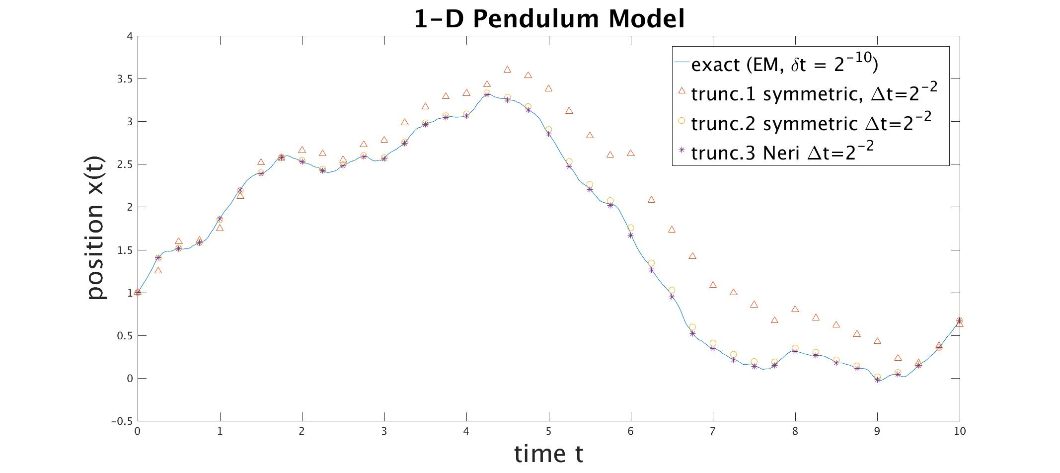
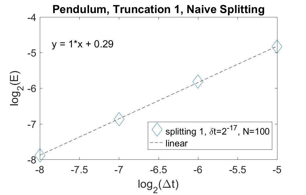
Refer to caption
Figure 1: A trajectory for the simple 1-d pendulum model, using different splitting methods , but the same reference trajectory of the driving Brownian motion.
Refer to caption
Refer to caption
Refer to caption
Refer to caption
Refer to caption
Figure 2: The error plot versus the time step for the pendulum model on the log-log scale. From top to bottom: Truncations I, II and III. The step sizes are Δt=24,25,,28Δ𝑡superscript24superscript25superscript28\Delta t=2^{-4},2^{-5},\dots,2^{-8}. The number N𝑁N denotes the number of realizations. Only four values of ΔtΔ𝑡\Delta{t} appear. Since we are only concerned with asymptotic behavior, we took ΔtΔ𝑡\Delta{t} as small as possible to obtain the theoretically correct convergence rates. For certain schemes, the values of ΔtΔ𝑡\Delta{t} needed to be made smaller for this to occur.

6.2 A Lennard-Jones cluster

The i𝑖ith component (i=1,,n𝑖1𝑛i=1,\dots,n) of the function f𝑓f in the Lennard-Jones model is given by

(110) fi(x)=ji,j=1n(12(1rij)136(1rij)7)rijrij,subscript𝑓𝑖𝑥superscriptsubscriptformulae-sequence𝑗𝑖𝑗1𝑛12superscript1subscript𝑟𝑖𝑗136superscript1subscript𝑟𝑖𝑗7subscript𝑟𝑖𝑗subscript𝑟𝑖𝑗f_{i}(x)=\sum_{j\neq i,j=1}^{n}\left(12\left(\frac{1}{r_{ij}}\right)^{13}-6\left(\frac{1}{r_{ij}}\right)^{7}\right)\frac{\vec{r}_{ij}}{r_{ij}},

where rij=xixj3subscript𝑟𝑖𝑗subscript𝑥𝑖subscript𝑥𝑗superscript3\vec{r}_{ij}=\vec{x}_{i}-\vec{x}_{j}\in\mathbb{R}^{3} and rij=rij2subscript𝑟𝑖𝑗subscriptnormsubscript𝑟𝑖𝑗2r_{ij}=\|\vec{r}_{ij}\|_{2}. For our simulations, we used seven particles x1,,x73subscript𝑥1subscript𝑥7superscript3x_{1},\dots,x_{7}\in\mathbb{R}^{3} and use x𝑥x to denote the vector (x1,,x7)21subscript𝑥1subscript𝑥7superscript21(x_{1},\dots,x_{7})\in\mathbb{R}^{21}, so that the total dimension n𝑛n is 21. Similarly, by v𝑣v we mean the vector (v1,,v7)21subscript𝑣1subscript𝑣7superscript21(v_{1},\dots,v_{7})\in\mathbb{R}^{21} of the velocities of each particle in all dimensions. We take Γ=10I21×21Γ10subscript𝐼2121\Gamma=10I_{21\times 21}, and σ=2kBTΓ𝜎2subscript𝑘𝐵𝑇Γ\sigma=\sqrt{2k_{B}T\Gamma}, where kBT=0.3subscript𝑘𝐵𝑇0.3k_{B}T=0.3, and T𝑇T is the temperature, not to be confused with the final time T𝑇T. Initially, the atoms are arranged at the vertices of a hexagon and its center. The side length corresponds to the minimum of the Lennard-Jones potential, 21/6.superscript2162^{1/6}. Notice that for this model, the function f(x)𝑓𝑥f(x) does not have bounded derivatives unless a cut-off is introduced. Nevertheless, as shown in Fig. 3, the strong order of accuracy is still consistent with the results of the analysis. We note that while the fifth method is indeed of order 3, the error is larger than for the method with order 2, as is the case with the pendulum model.
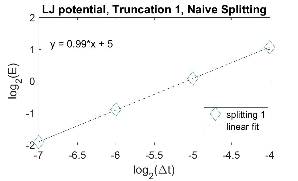
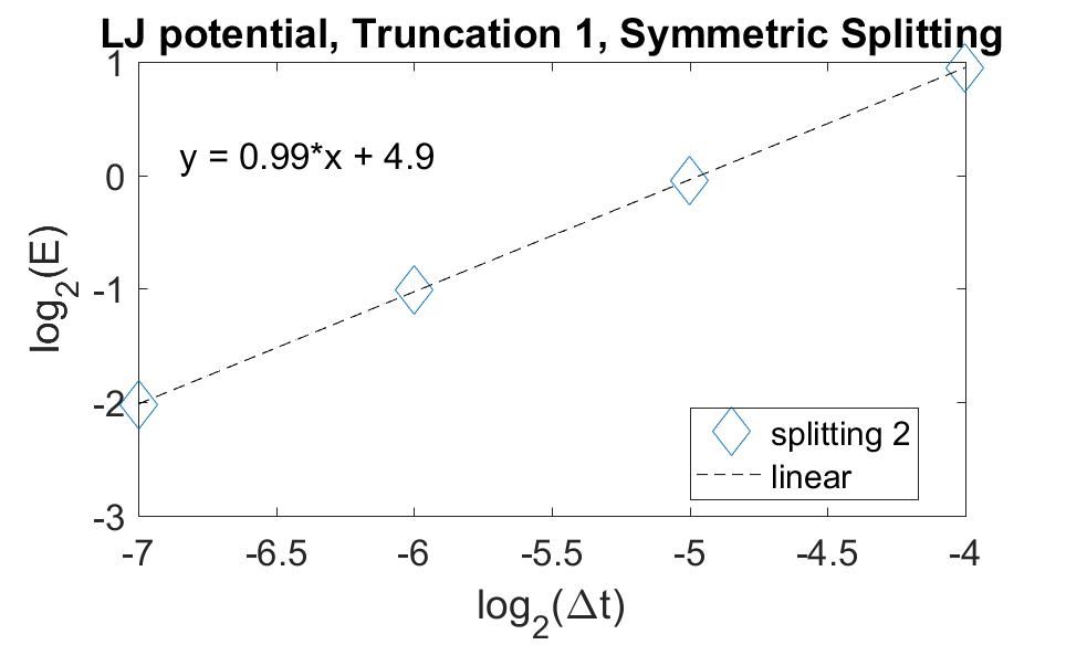
Refer to caption
Refer to caption
Refer to caption
Refer to caption
Refer to caption
Refer to caption
Figure 3: The error plot for the LJ-7 cluster on a log-log scale. From top to bottom: Truncations I, II and III, and the Stochastic velocity Verlet (SVV) method. The step sizes are Δt=24,25,,211Δ𝑡superscript24superscript25superscript211\Delta t=2^{-4},2^{-5},\dots,2^{-11}. The number N𝑁N denotes the number of realizations. Since we are only concerned with asymptotic behavior, we took ΔtΔ𝑡\Delta{t} as small as possible to obtain the theoretically correct convergence rates.For certain schemes, the values of ΔtΔ𝑡\Delta{t} needed to be made smaller for this to occur.

7 Summary and discussion

In this paper, we analyzed the strong convergence of some widely implemented schemes, and developed new operator-splitting schemes based on Kunita’s solution representation. In particular, we obtained algorithms with strong order up to order 3.This type of convergence is important for predicting the transient stage of the stochastic processes.

There are several remaining challenges in simulating algorithms for Langevin-type of equations. First [29], there might be multiple scales involved in the force term f(x)𝑓𝑥f(x). In this case, a more appropriate splitting [32] is between the fast and slow forces. Secondly, the damping and diffusion coefficients can be position-dependent. Such models arise, for instance, in the dissipative-particle dynamics (DPD) [35, 18]. Finally, there are Langevin equations with strong stiffness, e.g., large damping coefficients. In this case, implicit algorithm are needed. These issues will be addressed in separate works.

8 Appendix: derivation of Itô-Taylor expansions with strong convergence rates up to 3

Due to the lengthy calculations in the analysis, we have included some parts of the proofs in the appendix. These details are useful for the analysis.

8.1 SDE notation

An autonomous Itô stochastic differential equation or SDE can be written formally as,

(111) dz(t)=a(z(t))dt+b(z(t))dWt, 0tT,formulae-sequence𝑑𝑧𝑡𝑎𝑧𝑡𝑑𝑡𝑏𝑧𝑡𝑑subscript𝑊𝑡 0𝑡𝑇dz(t)=a(z(t))dt+b(z(t))dW_{t},\text{\quad}0\leq t\leq T,

which means that

(112) z(t)=z(0)+0ta(z(s))𝑑s+0tb(z(s))𝑑Ws, 0tT,formulae-sequence𝑧𝑡𝑧0superscriptsubscript0𝑡𝑎𝑧𝑠differential-d𝑠superscriptsubscript0𝑡𝑏𝑧𝑠differential-dsubscript𝑊𝑠 0𝑡𝑇z(t)=z(0)+\int_{0}^{t}a(z(s))ds+\int_{0}^{t}b(z(s))dW_{s},\text{\quad}0\leq t\leq T,

where 𝑑sdifferential-d𝑠\int ds denotes the usual Riemann integral and 𝑑Wsdifferential-dsubscript𝑊𝑠\int dW_{s} denotes the Itô stochastic integral, as defined in [24, Ch.3] for example, and the Wtsubscript𝑊𝑡W_{t} denotes a standard m𝑚m-dimensional Wiener process as defined in [24, Ch.2]. We use super-scripts for columns or entries. That is, a=(a1,,ad)𝑎superscript𝑎1superscript𝑎𝑑a=(a^{1},\dots,a^{d}), b=(bij)i,j=1d𝑏superscriptsubscriptsuperscript𝑏𝑖𝑗𝑖𝑗1𝑑b=(b^{ij})_{i,j=1}^{d}, bjsuperscript𝑏𝑗b^{j} is the j𝑗jth column of b𝑏b, and W=(W1,,Wm)𝑊superscript𝑊1superscript𝑊𝑚W=(W^{1},\dots,W^{m}). We call a=a(z):dd:𝑎𝑎𝑧superscript𝑑superscript𝑑a=a(z):\mathbb{R}^{d}\rightarrow\mathbb{R}^{d} the drift coefficient and b=b(z):dd×m:𝑏𝑏𝑧superscript𝑑superscript𝑑𝑚b=b(z):\mathbb{R}^{d}\rightarrow\mathbb{R}^{d\times m} the diffusion coefficient. If b𝑏b is constant we say the noise is additive; otherwise we call the noise multiplicative.

8.2 Langevin dynamics: notation

We consider the Langevin dynamics model as a decoupled system of 2n2𝑛2n SDEs,

(113) {dx(t)=v(t)dtdv(t)=(f(x(t))Γv(t))dt+σdW(t),cases𝑑𝑥𝑡absent𝑣𝑡𝑑𝑡𝑑𝑣𝑡absent𝑓𝑥𝑡Γ𝑣𝑡𝑑𝑡𝜎𝑑𝑊𝑡\begin{cases}dx(t)&=v(t)dt\\ dv(t)&=\left(f(x(t))-\Gamma v(t)\right)dt+\sigma dW(t),\end{cases}

with drift coefficient

(114) a=(vfΓv)2n𝑎matrix𝑣𝑓Γ𝑣superscript2𝑛a=\left(\begin{matrix}v\\ f-\Gamma v\end{matrix}\right)\in\mathbb{R}^{2n}

and constant diffusion coefficient

(115) b=(0σ)2n×n.𝑏matrix0𝜎superscript2𝑛𝑛b=\left(\begin{matrix}0\\ \sigma\end{matrix}\right)\in\mathbb{R}^{2n\times n}.

Here x,vn𝑥𝑣superscript𝑛x,v\in\mathbb{R}^{n} denote position and velocity vectors, Γ,σn×nΓ𝜎superscript𝑛𝑛\Gamma,\sigma\in\mathbb{R}^{n\times n} are square constant matrices denoting the friction and diffusion of the system, and Wn𝑊superscript𝑛W\in\mathbb{R}^{n} is the standard Wiener process. Since b𝑏b is constant, the noise is additive. The function f=f(x):nn:𝑓𝑓𝑥superscript𝑛superscript𝑛f=f(x):\mathbb{R}^{n}\rightarrow\mathbb{R}^{n} represents a conservative force depending only on position, which is generally non-linear, and we assume that all second order derivatives of f𝑓f exist.

8.3 Itô-Taylor expansion: notation

The Itô-Taylor expansion, see [11, Ch.5 and 10], can be viewed as a generalization of the deterministic Taylor expansion, and of the Itô formula. There are weak and strong types of the expansions but we will focus only on strong type in this paper because we are interested in strong convergence. We fix a uniform discretization 0=t0<t1<<tN=T0subscript𝑡0subscript𝑡1subscript𝑡𝑁𝑇0=t_{0}<t_{1}<\dots<t_{N}=T of the time interval [0,T]0𝑇[0,T] with steps tk=kΔtsubscript𝑡𝑘𝑘Δ𝑡t_{k}=k{\Delta t} and uniform step size Δt=T/N=tk+1tkΔ𝑡𝑇𝑁subscript𝑡𝑘1subscript𝑡𝑘{\Delta t}=T/N=t_{k+1}-t_{k} for k=0,1,,N1𝑘01𝑁1k=0,1,\dots,N-1.

Then, the strong Itô-Taylor expansion of order γ{0.5,1.0,1.5,2.0,2.5,3.0}𝛾0.51.01.52.02.53.0\gamma\in\{0.5,1.0,1.5,2.0,2.5,3.0\} is an explicit one-step method given by y0=z(t0)subscript𝑦0𝑧subscript𝑡0y_{0}=z(t_{0}) and for k=1,2,,N1𝑘12𝑁1k=1,2,\dots,N-1,

(116) yk+1=yk+α𝒜γgα(yk)Iα.subscript𝑦𝑘1subscript𝑦𝑘subscript𝛼subscript𝒜𝛾subscript𝑔𝛼subscript𝑦𝑘subscript𝐼𝛼y_{k+1}=y_{k}+\sum_{\alpha\in\mathcal{A}_{\gamma}}g_{\alpha}(y_{k})I_{\alpha}.

Here, 𝒜γsubscript𝒜𝛾\mathcal{A}_{\gamma} is a set of multi-indices α𝛼\alpha, gαsubscript𝑔𝛼g_{\alpha} are corresponding coefficient functions of yksubscript𝑦𝑘y_{k}, and Iαsubscript𝐼𝛼I_{\alpha} are corresponding Itô stochastic (defined also in [11, Ch.5]). In any case, we include the definitions below for completeness so that the reader can understand how we derive the expansions for the Langevin dynamics model.

Let \mathcal{M} denote the set of all multi-indices α=(j1,,jl)𝛼subscript𝑗1subscript𝑗𝑙\alpha=(j_{1},\dots,j_{l}) with entries j1,,jl{0,1,,m}subscript𝑗1subscript𝑗𝑙01𝑚j_{1},\dots,j_{l}\in\{0,1,\dots,m\}, length l(α):=lassign𝑙𝛼𝑙l(\alpha):=l, and number of zero entries n(α)𝑛𝛼n(\alpha). Then 𝒜γsubscript𝒜𝛾\mathcal{A}_{\gamma} is the subset given by,

(117) 𝒜γ:={α:l(α)+n(α)2γ or l(α)+n(α)=γ+0.5}.assignsubscript𝒜𝛾conditional-set𝛼𝑙𝛼𝑛𝛼2𝛾 or 𝑙𝛼𝑛𝛼𝛾0.5\mathcal{A}_{\gamma}:=\{\alpha\in\mathcal{M}:l(\alpha)+n(\alpha)\leq 2\gamma\text{ or }l(\alpha)+n(\alpha)=\gamma+0.5\}.

We will derive 𝒜γsubscript𝒜𝛾\mathcal{A}_{\gamma} for increasing γ=0.5,1.0,,3.0𝛾0.51.03.0\gamma=0.5,1.0,\dots,3.0, using the simple fact that 𝒜γ𝒜γ+0.5subscript𝒜𝛾subscript𝒜𝛾0.5\mathcal{A}_{\gamma}\subset\mathcal{A}_{\gamma+0.5}.

Turning now to the coefficient functions gαsubscript𝑔𝛼g_{\alpha}, we first define differential operators L0superscript𝐿0L^{0} and Ljsuperscript𝐿𝑗L^{j} for j=1,,m𝑗1𝑚j=1,\dots,m as follows:

(118) L0superscript𝐿0\displaystyle L^{0} =k=1nakzk+12k,l=1nj=1nbkjblj2zkzlabsentsuperscriptsubscript𝑘1𝑛superscript𝑎𝑘subscript𝑧𝑘12superscriptsubscript𝑘𝑙1𝑛superscriptsubscript𝑗1𝑛superscript𝑏𝑘𝑗superscript𝑏𝑙𝑗superscript2superscript𝑧𝑘superscript𝑧𝑙\displaystyle=\sum_{k=1}^{n}a^{k}\frac{\partial}{\partial z_{k}}+\frac{1}{2}\sum_{k,l=1}^{n}\sum_{j=1}^{n}b^{kj}b^{lj}\frac{\partial^{2}}{\partial z^{k}\partial z^{l}}
Ljsuperscript𝐿𝑗\displaystyle L^{j} =k=1nbkjzk j=1,,m.formulae-sequenceabsentsuperscriptsubscript𝑘1𝑛superscript𝑏𝑘𝑗subscript𝑧𝑘 𝑗1𝑚\displaystyle=\sum_{k=1}^{n}b^{kj}\frac{\partial}{\partial z_{k}}\text{\quad}j=1,\dots,m.

The coefficient function gαsubscript𝑔𝛼g_{\alpha} corresponding to α=(j1,,jl)𝛼subscript𝑗1subscript𝑗𝑙\alpha=(j_{1},\dots,j_{l})\in\mathcal{M} is given by,

(119) gα(z):=Lj1Lj2Ljl1bjlassignsubscript𝑔𝛼𝑧superscript𝐿subscript𝑗1superscript𝐿subscript𝑗2superscript𝐿subscript𝑗𝑙1superscript𝑏subscript𝑗𝑙g_{\alpha}(z):=L^{j_{1}}L^{j_{2}}\dots L^{j_{l-1}}b^{j_{l}}

where b0:=aassignsuperscript𝑏0𝑎b^{0}:=a. For the Langevin dynamics model we consider, these operators can be rewritten as,

(120) L0superscript𝐿0\displaystyle L^{0} =k=1nvkxk+k=1n{f(x)Γv}kvk+12k,l=1nj=1nσkjσlj2vkvlabsentsuperscriptsubscript𝑘1𝑛superscript𝑣𝑘superscript𝑥𝑘superscriptsubscript𝑘1𝑛superscript𝑓𝑥Γ𝑣𝑘superscript𝑣𝑘12superscriptsubscript𝑘𝑙1𝑛superscriptsubscript𝑗1𝑛superscript𝜎𝑘𝑗superscript𝜎𝑙𝑗superscript2superscript𝑣𝑘superscript𝑣𝑙\displaystyle=\sum_{k=1}^{n}v^{k}\frac{\partial}{\partial x^{k}}+\sum_{k=1}^{n}\{f(x)-\Gamma v\}^{k}\frac{\partial}{\partial v^{k}}+\frac{1}{2}\sum_{k,l=1}^{n}\sum_{j=1}^{n}\sigma^{kj}\sigma^{lj}\frac{\partial^{2}}{\partial v^{k}\partial v^{l}}
Ljsuperscript𝐿𝑗\displaystyle L^{j} =k=1nσkjvk.absentsuperscriptsubscript𝑘1𝑛superscript𝜎𝑘𝑗superscript𝑣𝑘\displaystyle=\sum_{k=1}^{n}\sigma^{kj}\frac{\partial}{\partial v^{k}}.

Finally, the stochastic integrals Iαsubscript𝐼𝛼I_{\alpha} are given by,

(121) Iα:=0Δt0sl0s30s2𝑑u(s1)𝑑u(s2)𝑑u(sl1)𝑑u(sl)assignsubscript𝐼𝛼superscriptsubscript0Δ𝑡superscriptsubscript0subscript𝑠𝑙superscriptsubscript0subscript𝑠3superscriptsubscript0subscript𝑠2differential-d𝑢subscript𝑠1differential-d𝑢subscript𝑠2differential-d𝑢subscript𝑠𝑙1differential-d𝑢subscript𝑠𝑙I_{\alpha}:=\int_{0}^{{\Delta t}}\int_{0}^{s_{l}}\dots\int_{0}^{s_{3}}\int_{0}^{s_{2}}du(s_{1})du(s_{2})\dots du(s_{l-1})du(s_{l})

where each du(si)𝑑𝑢subscript𝑠𝑖du(s_{i}) is given by,

(122) du(si)={dsi if ji=0dWsiji if ji{1,,m}.𝑑𝑢subscript𝑠𝑖cases𝑑subscript𝑠𝑖 if subscript𝑗𝑖0𝑑superscriptsubscript𝑊subscript𝑠𝑖subscript𝑗𝑖 if subscript𝑗𝑖1𝑚du(s_{i})=\begin{cases}ds_{i}&\text{ if }j_{i}=0\\ dW_{s_{i}}^{j_{i}}&\text{ if }j_{i}\in\{1,\dots,m\}.\end{cases}

8.4 Itô-Taylor expansions with strong orders γ=0.5,1.0,1.5,2.0,2.5,𝛾0.51.01.52.02.5\gamma=0.5,1.0,1.5,2.0,2.5, and 3

First we compute the multi-index sets 𝒜γsubscript𝒜𝛾\mathcal{A}_{\gamma}. For γ=0.5𝛾0.5\gamma=0.5, we make the simple calculation,

(123) 𝒜0.5subscript𝒜0.5\displaystyle\mathcal{A}_{0.5} ={α:l(α)+n(α)1 or l(α)=n(α)=1}absentconditional-set𝛼𝑙𝛼𝑛𝛼1 or 𝑙𝛼𝑛𝛼1\displaystyle=\{\alpha:l(\alpha)+n(\alpha)\leq 1\text{ or }l(\alpha)=n(\alpha)=1\}
={(0),(j):j=1,,m}.absentconditional-set0𝑗𝑗1𝑚\displaystyle=\{(0),(j):j=1,\dots,m\}.

The corresponding coefficient functions are,

(124) g(0)=b0=a=(vfγv)subscript𝑔0superscript𝑏0𝑎matrix𝑣𝑓𝛾𝑣g_{(0)}=b^{0}=a=\left(\begin{matrix}v\\ f-\gamma v\end{matrix}\right)

and

(125) g(j)=bj=(0σj), j=1,,m.formulae-sequencesubscript𝑔𝑗superscript𝑏𝑗matrix0superscript𝜎𝑗 𝑗1𝑚g_{(j)}=b^{j}=\left(\begin{matrix}0\\ \sigma^{j}\end{matrix}\right),\text{\quad}j=1,\dots,m.

The corresponding stochastic integrals Iαsubscript𝐼𝛼I_{\alpha} are,

(126) I(0)=0Δtds1=Δt and I(j)=0ΔtdWs1j=WΔtj=:ΔWj.I_{(0)}=\int_{0}^{{\Delta t}}ds_{1}={\Delta t}\text{\quad and\quad}I_{(j)}=\int_{0}^{{\Delta t}}dW_{s_{1}}^{j}=W_{{\Delta t}}^{j}=:\Delta W^{j}.

Thus, the strong order γ=0.5𝛾0.5\gamma=0.5 Itô-Taylor expansion is,

(127) yk+1=yk+(vfγv)Δt+j=1m(0σj)ΔWj,subscript𝑦𝑘1subscript𝑦𝑘matrix𝑣𝑓𝛾𝑣Δ𝑡superscriptsubscript𝑗1𝑚matrix0superscript𝜎𝑗Δsuperscript𝑊𝑗y_{k+1}=y_{k}+\left(\begin{matrix}v\\ f-\gamma v\end{matrix}\right){\Delta t}+\sum_{j=1}^{m}\left(\begin{matrix}0\\ \sigma^{j}\end{matrix}\right)\Delta W^{j},

which is also called the Euler or Euler-Maruyama method. As usual σjdsuperscript𝜎𝑗superscript𝑑\sigma^{j}\in\mathbb{R}^{d} denotes the j𝑗jth column of σd×m𝜎superscript𝑑𝑚\sigma\in\mathbb{R}^{d\times m}, evaluated at xkdsubscript𝑥𝑘superscript𝑑x_{k}\in\mathbb{R}^{d}.

For γ=1.0𝛾1.0\gamma=1.0, we calculate

(128) 𝒜1={α:l(α)+n(α)2},subscript𝒜1conditional-set𝛼𝑙𝛼𝑛𝛼2\mathcal{A}_{1}=\{\alpha:l(\alpha)+n(\alpha)\leq 2\},

observing that the equation l(α)=n(α)=1.5𝑙𝛼𝑛𝛼1.5l(\alpha)=n(\alpha)=1.5 is never satisfied. We have

(129) 𝒜1={(0),(j1),(j1,j2):j1,j2=1,,m},subscript𝒜1conditional-set0subscript𝑗1subscript𝑗1subscript𝑗2formulae-sequencesubscript𝑗1subscript𝑗21𝑚\mathcal{A}_{1}=\{(0),(j_{1}),(j_{1},j_{2}):j_{1},j_{2}=1,\dots,m\},

which is 𝒜0.5subscript𝒜0.5\mathcal{A}_{0.5} plus (j1,j2)subscript𝑗1subscript𝑗2(j_{1},j_{2}) for j1,j2=1,,mformulae-sequencesubscript𝑗1subscript𝑗21𝑚j_{1},j_{2}=1,\dots,m. The new coefficient functions g(j1,j2)subscript𝑔subscript𝑗1subscript𝑗2g_{(j_{1},j_{2})} are identically zero. Indeed,

(130) g(j1,j2)=Lj1bj2=(Lj1(0)Lj1(σj2))=02d,subscript𝑔subscript𝑗1subscript𝑗2superscript𝐿subscript𝑗1superscript𝑏subscript𝑗2matrixsuperscript𝐿subscript𝑗10superscript𝐿subscript𝑗1superscript𝜎subscript𝑗20superscript2𝑑g_{(j_{1},j_{2})}=L^{j_{1}}b^{j_{2}}=\left(\begin{matrix}L^{j_{1}}(0)\\ L^{j_{1}}(\sigma^{j_{2}})\end{matrix}\right)=0\in\mathbb{R}^{2d},

due to the additive noise. Therefore, the strong order γ=1.0𝛾1.0\gamma=1.0 Itô-Taylor expansion is the same as the one with strong order γ=0.5𝛾0.5\gamma=0.5.

Consider γ=1.5𝛾1.5\gamma=1.5. By definition,

(131) 𝒜1.5={α:l(α)+n(α)3 or l(α)=n(α)=2}.subscript𝒜1.5conditional-set𝛼𝑙𝛼𝑛𝛼3 or 𝑙𝛼𝑛𝛼2\mathcal{A}_{1.5}=\{\alpha:l(\alpha)+n(\alpha)\leq 3\text{ or }l(\alpha)=n(\alpha)=2\}.

Since 𝒜1𝒜1.5subscript𝒜1subscript𝒜1.5\mathcal{A}_{1}\subset\mathcal{A}_{1.5}, we just need to find those α𝛼\alpha for which either l(α)+n(α)=3𝑙𝛼𝑛𝛼3l(\alpha)+n(\alpha)=3 or l(α)=n(α)=2𝑙𝛼𝑛𝛼2l(\alpha)=n(\alpha)=2. We list them now:

(132) (j1,j2,j3), (0,j1), (j1,0), and (0,0).subscript𝑗1subscript𝑗2subscript𝑗3 0subscript𝑗1 subscript𝑗10 and 00(j_{1},j_{2},j_{3}),\text{\quad}(0,j_{1}),\text{\quad}(j_{1},0),\text{\quad and\quad}(0,0).

Fortunately g(j1,j2,j3)=0subscript𝑔subscript𝑗1subscript𝑗2subscript𝑗30g_{(j_{1},j_{2},j_{3})}=0 for j1,j2,j3=1,,mformulae-sequencesubscript𝑗1subscript𝑗2subscript𝑗31𝑚j_{1},j_{2},j_{3}=1,\dots,m, because g(j1,j2,j3)=Lj1g(j2,j3)subscript𝑔subscript𝑗1subscript𝑗2subscript𝑗3superscript𝐿subscript𝑗1subscript𝑔subscript𝑗2subscript𝑗3g_{(j_{1},j_{2},j_{3})}=L^{j_{1}}g_{(j_{2},j_{3})} and g(j2,j3)=0subscript𝑔subscript𝑗2subscript𝑗30g_{(j_{2},j_{3})}=0. Thus the multi-indices (j1,j2,j3)subscript𝑗1subscript𝑗2subscript𝑗3(j_{1},j_{2},j_{3}) make no contribution to the expansion. In addition, due to the additive noise the coefficient functions g(0,j)subscript𝑔0𝑗g_{(0,j)} are identically zero as well. Indeed,

(133) g(0,j)=L0bj=0subscript𝑔0𝑗superscript𝐿0superscript𝑏𝑗0g_{(0,j)}=L^{0}b^{j}=0

since bj=(0,σj)superscript𝑏𝑗0superscript𝜎𝑗b^{j}=(0,\sigma^{j}) is constant. On the other hand, we calculate the non-trivial coefficient functions:

(134) g(j,0)subscript𝑔𝑗0\displaystyle g_{(j,0)} =Lja=(LjvLjfγv)=(σjγσj),absentsuperscript𝐿𝑗𝑎matrixsuperscript𝐿𝑗𝑣superscript𝐿𝑗𝑓𝛾𝑣matrixsuperscript𝜎𝑗𝛾superscript𝜎𝑗\displaystyle=L^{j}a=\left(\begin{matrix}L^{j}v\\ L^{j}f-\gamma v\end{matrix}\right)=\left(\begin{matrix}\sigma^{j}\\ -\gamma\sigma^{j}\end{matrix}\right),
g(0,0)subscript𝑔00\displaystyle g_{(0,0)} =L0a=(L0vL0{fγv})=(fγvx(f)vγ{fγv}).absentsuperscript𝐿0𝑎matrixsuperscript𝐿0𝑣superscript𝐿0𝑓𝛾𝑣matrix𝑓𝛾𝑣subscript𝑥𝑓𝑣𝛾𝑓𝛾𝑣\displaystyle=L^{0}a=\left(\begin{matrix}L^{0}v\\ L^{0}\{f-\gamma v\}\end{matrix}\right)=\left(\begin{matrix}f-\gamma v\\ \nabla_{x}(f)v-\gamma\{f-\gamma v\}\end{matrix}\right).

The corresponding Itô integrals are:

(135) I(j,0)subscript𝐼𝑗0\displaystyle I_{(j,0)} =0Δt0s2𝑑Ws1j𝑑s=0ΔtWs𝑑sabsentsuperscriptsubscript0Δ𝑡superscriptsubscript0subscript𝑠2differential-dsuperscriptsubscript𝑊subscript𝑠1𝑗differential-d𝑠superscriptsubscript0Δ𝑡subscript𝑊𝑠differential-d𝑠\displaystyle=\int_{0}^{{\Delta t}}\int_{0}^{s_{2}}dW_{s_{1}}^{j}ds=\int_{0}^{{\Delta t}}W_{s}ds
(136) I(0,0)subscript𝐼00\displaystyle I_{(0,0)} =0Δt0s2𝑑s1𝑑s2=Δt22.absentsuperscriptsubscript0Δ𝑡superscriptsubscript0subscript𝑠2differential-dsubscript𝑠1differential-dsubscript𝑠2Δsuperscript𝑡22\displaystyle=\int_{0}^{{\Delta t}}\int_{0}^{s_{2}}ds_{1}ds_{2}=\frac{{\Delta t}^{2}}{2}.

Thus, the strong order γ=1.5𝛾1.5\gamma=1.5 Itô-Taylor expansion is,

(137) yk+1subscript𝑦𝑘1\displaystyle y_{k+1} =yk+(vfγv)Δt+j=1m(0σj)ΔWjabsentsubscript𝑦𝑘matrix𝑣𝑓𝛾𝑣Δ𝑡superscriptsubscript𝑗1𝑚matrix0superscript𝜎𝑗Δsuperscript𝑊𝑗\displaystyle=y_{k}+\left(\begin{matrix}v\\ f-\gamma v\end{matrix}\right){\Delta t}+\sum_{j=1}^{m}\left(\begin{matrix}0\\ \sigma^{j}\end{matrix}\right)\Delta W^{j}
(138) +j=1m(σjγσj)0ΔtWsj𝑑ssuperscriptsubscript𝑗1𝑚matrixsuperscript𝜎𝑗𝛾superscript𝜎𝑗superscriptsubscript0Δ𝑡superscriptsubscript𝑊𝑠𝑗differential-d𝑠\displaystyle+\sum_{j=1}^{m}\left(\begin{matrix}\sigma^{j}\\ -\gamma\sigma^{j}\end{matrix}\right)\int_{0}^{{\Delta t}}W_{s}^{j}ds
(139) +(fγvx(f)vγ{fγv})Δt22.matrix𝑓𝛾𝑣subscript𝑥𝑓𝑣𝛾𝑓𝛾𝑣Δsuperscript𝑡22\displaystyle+\left(\begin{matrix}f-\gamma v\\ \nabla_{x}(f)v-\gamma\{f-\gamma v\}\end{matrix}\right)\frac{{\Delta t}^{2}}{2}.

The notation x(f)subscript𝑥𝑓\nabla_{x}(f) denotes the d×d𝑑𝑑d\times d Jacobian matrix of f𝑓f evaluated at xksubscript𝑥𝑘x_{k}, with derivatives taken with respect to x𝑥x.

We move on to γ=2.0𝛾2.0\gamma=2.0. The hierarchical set 𝒜2subscript𝒜2\mathcal{A}_{2} is,

(140) 𝒜2={α:l(α)+n(α)4},subscript𝒜2conditional-set𝛼𝑙𝛼𝑛𝛼4\mathcal{A}_{2}=\{\alpha:l(\alpha)+n(\alpha)\leq 4\},

noting that the equation l(α)=n(α)=2.5𝑙𝛼𝑛𝛼2.5l(\alpha)=n(\alpha)=2.5 is never satisfied. We also recall that 𝒜1.5𝒜2subscript𝒜1.5subscript𝒜2\mathcal{A}_{1.5}\subset\mathcal{A}_{2}, and so we need only look for new multi-indices α𝛼\alpha which satisfy l(α)+n(α)=4𝑙𝛼𝑛𝛼4l(\alpha)+n(\alpha)=4, which are,

(141) (j1,j2,0), (j1,0,j2), (0,j1,j2), and (j1,j2,j3), for j1,j2,j3=1,,m.formulae-sequencesubscript𝑗1subscript𝑗20 subscript𝑗10subscript𝑗2 0subscript𝑗1subscript𝑗2 and subscript𝑗1subscript𝑗2subscript𝑗3 for subscript𝑗1subscript𝑗2subscript𝑗31𝑚(j_{1},j_{2},0),\text{\quad}(j_{1},0,j_{2}),\text{\quad}(0,j_{1},j_{2}),\text{\quad and\quad}(j_{1},j_{2},j_{3}),\text{\quad for }j_{1},j_{2},j_{3}=1,\dots,m.

The coefficient functions g(0,j1,j2)subscript𝑔0subscript𝑗1subscript𝑗2g_{(0,j_{1},j_{2})} and g(j1,j2,j3)subscript𝑔subscript𝑗1subscript𝑗2subscript𝑗3g_{(j_{1},j_{2},j_{3})} are identically zero, since g(j1,j2)subscript𝑔subscript𝑗1subscript𝑗2g_{(j_{1},j_{2})} is zero. In addition, g(j1,j2,0)=0subscript𝑔subscript𝑗1subscript𝑗200g_{(j_{1},j_{2},0)}=0 because g(j,0)=(σj,γσj)subscript𝑔𝑗0superscript𝜎𝑗𝛾superscript𝜎𝑗g_{(j,0)}=(\sigma^{j},-\gamma\sigma^{j}) is constant. That leaves us only with g(j1,0,j2)subscript𝑔subscript𝑗10subscript𝑗2g_{(j_{1},0,j_{2})}, which is also zero because g(0,j2)=0subscript𝑔0subscript𝑗20g_{(0,j_{2})}=0.

(142) g(j1,0,j2)=Lj1g(0,j2)=(Lj10Lj1x(σj2)v)=(0x(σj2)σj1).subscript𝑔subscript𝑗10subscript𝑗2superscript𝐿subscript𝑗1subscript𝑔0subscript𝑗2matrixsuperscript𝐿subscript𝑗10superscript𝐿subscript𝑗1subscript𝑥superscript𝜎subscript𝑗2𝑣matrix0subscript𝑥superscript𝜎subscript𝑗2superscript𝜎subscript𝑗1g_{(j_{1},0,j_{2})}=L^{j_{1}}g_{(0,j_{2})}=\left(\begin{matrix}L^{j_{1}}0\\ L^{j_{1}}\nabla_{x}(\sigma^{j_{2}})v\end{matrix}\right)=\left(\begin{matrix}0\\ \nabla_{x}(\sigma^{j_{2}})\sigma^{j_{1}}\end{matrix}\right).

Therefore there are no new non-trivial coefficient functions, and thus the strong order γ=2.0𝛾2.0\gamma=2.0 Itô-Taylor expansion is the same as the one with order γ=1.5𝛾1.5\gamma=1.5.

As for γ=2.5𝛾2.5\gamma=2.5, we calculate

(143) 𝒜2.5𝒜2subscript𝒜2.5subscript𝒜2\displaystyle\mathcal{A}_{2.5}-\mathcal{A}_{2} ={α𝒜2.5:α𝒜2}absentconditional-set𝛼subscript𝒜2.5𝛼subscript𝒜2\displaystyle=\{\alpha\in\mathcal{A}_{2.5}:\alpha\notin\mathcal{A}_{2}\}
={(0,0,j1),(0,j1,0),(j1,0,0),(0,0,0)\displaystyle=\{(0,0,j_{1}),(0,j_{1},0),(j_{1},0,0),(0,0,0)
(j1,j2,j3,0),(j1,j2,0,j3),(j1,0,j2,j3),(0,j1,j2,j3)subscript𝑗1subscript𝑗2subscript𝑗30subscript𝑗1subscript𝑗20subscript𝑗3subscript𝑗10subscript𝑗2subscript𝑗30subscript𝑗1subscript𝑗2subscript𝑗3\displaystyle(j_{1},j_{2},j_{3},0),(j_{1},j_{2},0,j_{3}),(j_{1},0,j_{2},j_{3}),(0,j_{1},j_{2},j_{3})
(j1,j2,j3,j4,j5):ji=1,,m and i=1,,5}.\displaystyle(j_{1},j_{2},j_{3},j_{4},j_{5}):j_{i}=1,\dots,m\text{ and }i=1,\dots,5\}.

Next we find the vanishing coefficient functions gα=0subscript𝑔𝛼0g_{\alpha}=0 for α𝒜2.5𝒜2𝛼subscript𝒜2.5subscript𝒜2\alpha\in\mathcal{A}_{2.5}-\mathcal{A}_{2} in the case m=1𝑚1m=1, which generalizes naturally to m>1𝑚1m>1. Since g(1)=b=(0,σ)subscript𝑔1𝑏0𝜎g_{(1)}=b=(0,\sigma) is constant, the coefficient functions g(0,0,1),g(1,1,0,1),g(0,1,1,1),g(1,1,1,1,1)subscript𝑔001subscript𝑔1101subscript𝑔0111subscript𝑔11111g_{(0,0,1)},g_{(1,1,0,1)},g_{(0,1,1,1)},g_{(1,1,1,1,1)} vanish:

(144) g(0,0,1)subscript𝑔001\displaystyle g_{(0,0,1)} =L0L0g(1)=0absentsuperscript𝐿0superscript𝐿0subscript𝑔10\displaystyle=L^{0}L^{0}g_{(1)}=0
(145) g(1,1,0,1)subscript𝑔1101\displaystyle g_{(1,1,0,1)} =L1L1L0g(1)=0absentsuperscript𝐿1superscript𝐿1superscript𝐿0subscript𝑔10\displaystyle=L^{1}L^{1}L^{0}g_{(1)}=0
(146) g(1,0,1,1)subscript𝑔1011\displaystyle g_{(1,0,1,1)} =L1L0L1g(1)=0absentsuperscript𝐿1superscript𝐿0superscript𝐿1subscript𝑔10\displaystyle=L^{1}L^{0}L^{1}g_{(1)}=0
(147) g(0,1,1,1)subscript𝑔0111\displaystyle g_{(0,1,1,1)} =L0L1L1g(1)=0absentsuperscript𝐿0superscript𝐿1superscript𝐿1subscript𝑔10\displaystyle=L^{0}L^{1}L^{1}g_{(1)}=0
(148) g(1,1,1,1,1)subscript𝑔11111\displaystyle g_{(1,1,1,1,1)} =L1L1L1L1g(1)=0.absentsuperscript𝐿1superscript𝐿1superscript𝐿1superscript𝐿1subscript𝑔10\displaystyle=L^{1}L^{1}L^{1}L^{1}g_{(1)}=0.

What about the indices α=(1,1,1,0),(0,1,0),(1,0,0)𝛼1110010100\alpha=(1,1,1,0),(0,1,0),(1,0,0) and (0,0,0)000(0,0,0)? Well, we have already seen that g(1,0)=(σ,γσ)subscript𝑔10𝜎𝛾𝜎g_{(1,0)}=(\sigma,-\gamma\sigma) is constant. Therefore, g(1,1,1,0)=g(0,1,0)=0subscript𝑔1110subscript𝑔0100g_{(1,1,1,0)}=g_{(0,1,0)}=0, since

(149) g(1,1,1,0)subscript𝑔1110\displaystyle g_{(1,1,1,0)} =L1L1g(1,0)=0absentsuperscript𝐿1superscript𝐿1subscript𝑔100\displaystyle=L^{1}L^{1}g_{(1,0)}=0
(150) g(0,1,0)subscript𝑔010\displaystyle g_{(0,1,0)} =L0g(1,0)=0.absentsuperscript𝐿0subscript𝑔100\displaystyle=L^{0}g_{(1,0)}=0.

We have two indices remaining: α=(1,0,0)𝛼100\alpha=(1,0,0) and (0,0,0)000(0,0,0), and the corresponding coefficient functions do not vanish, as we will see. We recall that,

(151) g(0,0)subscript𝑔00\displaystyle g_{(0,0)} =(fγvfvγ{fγv})absentmatrix𝑓𝛾𝑣superscript𝑓𝑣𝛾𝑓𝛾𝑣\displaystyle=\left(\begin{matrix}f-\gamma v\\ f^{\prime}v-\gamma\{f-\gamma v\}\end{matrix}\right)

for additive noise, and the differential operators are,

(152) L0superscript𝐿0\displaystyle L^{0} =vx+{fγv}vabsent𝑣subscript𝑥𝑓𝛾𝑣subscript𝑣\displaystyle=v\partial_{x}+\{f-\gamma v\}\partial_{v}
(153) L1superscript𝐿1\displaystyle L^{1} =σv.absent𝜎subscript𝑣\displaystyle=\sigma\partial_{v}.

Therefore,

(154) g(1,0,0)subscript𝑔100\displaystyle g_{(1,0,0)} =L1g(0,0)absentsuperscript𝐿1subscript𝑔00\displaystyle=L^{1}g_{(0,0)}
(155) =(σv{fγv}σv(fvγ{fγv}))absentmatrix𝜎subscript𝑣𝑓𝛾𝑣𝜎subscript𝑣superscript𝑓𝑣𝛾𝑓𝛾𝑣\displaystyle=\left(\begin{matrix}\sigma\partial_{v}\{f-\gamma v\}\\ \sigma\partial_{v}\left(f^{\prime}v-\gamma\{f-\gamma v\}\right)\end{matrix}\right)
(156) =(γσfσ+γ2σ),absentmatrix𝛾𝜎superscript𝑓𝜎superscript𝛾2𝜎\displaystyle=\left(\begin{matrix}-\gamma\sigma\\ f^{\prime}\sigma+\gamma^{2}\sigma\end{matrix}\right),

and

(157) g(0,0,0)subscript𝑔000\displaystyle g_{(0,0,0)} =L0g(0,0)absentsuperscript𝐿0subscript𝑔00\displaystyle=L^{0}g_{(0,0)}
(158) =(vx(fγv)+{fγv}v(fγv)vx[fvγ{fγv}]+{fγv}v[fvγ{fγv}])absentmatrix𝑣subscript𝑥𝑓𝛾𝑣𝑓𝛾𝑣subscript𝑣𝑓𝛾𝑣𝑣subscript𝑥delimited-[]superscript𝑓𝑣𝛾𝑓𝛾𝑣𝑓𝛾𝑣subscript𝑣delimited-[]superscript𝑓𝑣𝛾𝑓𝛾𝑣\displaystyle=\left(\begin{matrix}v\partial_{x}(f-\gamma v)+\{f-\gamma v\}\partial_{v}(f-\gamma v)\\ v\partial_{x}[f^{\prime}v-\gamma\{f-\gamma v\}]+\{f-\gamma v\}\partial_{v}[f^{\prime}v-\gamma\{f-\gamma v\}]\end{matrix}\right)
(159) =(fvγ{fγv}f′′v2γfv+f{fγv}+σ2{fγv}).absentmatrixsuperscript𝑓𝑣𝛾𝑓𝛾𝑣superscript𝑓′′superscript𝑣2𝛾superscript𝑓𝑣superscript𝑓𝑓𝛾𝑣superscript𝜎2𝑓𝛾𝑣\displaystyle=\left(\begin{matrix}f^{\prime}v-\gamma\{f-\gamma v\}\\ f^{\prime\prime}v^{2}-\gamma f^{\prime}v+f^{\prime}\{f-\gamma v\}+\sigma^{2}\{f-\gamma v\}\end{matrix}\right).

The corresponding functions for the case m>1𝑚1m>1 are,

(160) g(j,0,0)subscript𝑔𝑗00\displaystyle g_{(j,0,0)} =(γσjx(f)σj+γ2σj) andabsentmatrix𝛾superscript𝜎𝑗subscript𝑥𝑓superscript𝜎𝑗superscript𝛾2superscript𝜎𝑗 and\displaystyle=\left(\begin{matrix}-\gamma\sigma^{j}\\ \nabla_{x}(f)\sigma^{j}+\gamma^{2}\sigma^{j}\end{matrix}\right)\text{\quad and}
(161) g(0,0,0)subscript𝑔000\displaystyle g_{(0,0,0)} =(x(f)vγ{fγv}x[x(f)v]vγx(f)v+x(f){fγv}+σ2{fγv}),absentmatrixsubscript𝑥𝑓𝑣𝛾𝑓𝛾𝑣subscript𝑥subscript𝑥𝑓𝑣𝑣𝛾subscript𝑥𝑓𝑣subscript𝑥𝑓𝑓𝛾𝑣superscript𝜎2𝑓𝛾𝑣\displaystyle=\left(\begin{matrix}\nabla_{x}(f)v-\gamma\{f-\gamma v\}\\ \nabla_{x}[\nabla_{x}(f)v]v-\gamma\nabla_{x}(f)v+\nabla_{x}(f)\{f-\gamma v\}+\sigma^{2}\{f-\gamma v\}\end{matrix}\right),

which is a straightforward, but mildly unpleasant calculation. The related stochastic Itô integrals are,

(162) I(1,0,0)subscript𝐼100\displaystyle I_{(1,0,0)} =0Δt0s30s2𝑑Ws1𝑑s2𝑑s3 andabsentsuperscriptsubscript0Δ𝑡superscriptsubscript0subscript𝑠3superscriptsubscript0subscript𝑠2differential-dsubscript𝑊subscript𝑠1differential-dsubscript𝑠2differential-dsubscript𝑠3 and\displaystyle=\int_{0}^{{\Delta t}}\int_{0}^{s_{3}}\int_{0}^{s_{2}}dW_{s_{1}}ds_{2}ds_{3}\text{\quad and}
(163) I(0,0,0)subscript𝐼000\displaystyle I_{(0,0,0)} =0Δt0s30s2𝑑Ws1𝑑s2𝑑s3=Δt33!.absentsuperscriptsubscript0Δ𝑡superscriptsubscript0subscript𝑠3superscriptsubscript0subscript𝑠2differential-dsubscript𝑊subscript𝑠1differential-dsubscript𝑠2differential-dsubscript𝑠3Δsuperscript𝑡33\displaystyle=\int_{0}^{{\Delta t}}\int_{0}^{s_{3}}\int_{0}^{s_{2}}dW_{s_{1}}ds_{2}ds_{3}=\frac{{\Delta t}^{3}}{3!}.

Now we can add these terms to the strong order γ=2𝛾2\gamma=2 expansion to get the one with strong order γ=2.5𝛾2.5\gamma=2.5:

(164) yk+1subscript𝑦𝑘1\displaystyle y_{k+1} =yk+(vfγv)Δt+j=1m(0σj)ΔWjabsentsubscript𝑦𝑘matrix𝑣𝑓𝛾𝑣Δ𝑡superscriptsubscript𝑗1𝑚matrix0superscript𝜎𝑗Δsuperscript𝑊𝑗\displaystyle=y_{k}+\left(\begin{matrix}v\\ f-\gamma v\end{matrix}\right){\Delta t}+\sum_{j=1}^{m}\left(\begin{matrix}0\\ \sigma^{j}\end{matrix}\right)\Delta W^{j}
(165) +j=1m(σjγσj)0ΔtWsj𝑑ssuperscriptsubscript𝑗1𝑚matrixsuperscript𝜎𝑗𝛾superscript𝜎𝑗superscriptsubscript0Δ𝑡superscriptsubscript𝑊𝑠𝑗differential-d𝑠\displaystyle+\sum_{j=1}^{m}\left(\begin{matrix}\sigma^{j}\\ -\gamma\sigma^{j}\end{matrix}\right)\int_{0}^{{\Delta t}}W_{s}^{j}ds
(166) +(fγvx(f)vγ{fγv})Δt22matrix𝑓𝛾𝑣subscript𝑥𝑓𝑣𝛾𝑓𝛾𝑣Δsuperscript𝑡22\displaystyle+\left(\begin{matrix}f-\gamma v\\ \nabla_{x}(f)v-\gamma\{f-\gamma v\}\end{matrix}\right)\frac{{\Delta t}^{2}}{2}
(167) +j=1m(γσjx(f)σj+γ2σj)0Δt0s30s2𝑑Ws1j𝑑s2𝑑s3superscriptsubscript𝑗1𝑚matrix𝛾superscript𝜎𝑗subscript𝑥𝑓superscript𝜎𝑗superscript𝛾2superscript𝜎𝑗superscriptsubscript0Δ𝑡superscriptsubscript0subscript𝑠3superscriptsubscript0subscript𝑠2differential-dsuperscriptsubscript𝑊subscript𝑠1𝑗differential-dsubscript𝑠2differential-dsubscript𝑠3\displaystyle+\sum_{j=1}^{m}\left(\begin{matrix}-\gamma\sigma^{j}\\ \nabla_{x}(f)\sigma^{j}+\gamma^{2}\sigma^{j}\end{matrix}\right)\int_{0}^{{\Delta t}}\int_{0}^{s_{3}}\int_{0}^{s_{2}}dW_{s_{1}}^{j}ds_{2}ds_{3}
(168) +(x(f)vγ{fγv}x[x(f)v]vγx(f)v+x(f){fγv}+σ2{fγv})Δt33!.matrixsubscript𝑥𝑓𝑣𝛾𝑓𝛾𝑣subscript𝑥subscript𝑥𝑓𝑣𝑣𝛾subscript𝑥𝑓𝑣subscript𝑥𝑓𝑓𝛾𝑣superscript𝜎2𝑓𝛾𝑣Δsuperscript𝑡33\displaystyle+\left(\begin{matrix}\nabla_{x}(f)v-\gamma\{f-\gamma v\}\\ \nabla_{x}[\nabla_{x}(f)v]v-\gamma\nabla_{x}(f)v+\nabla_{x}(f)\{f-\gamma v\}+\sigma^{2}\{f-\gamma v\}\end{matrix}\right)\frac{{\Delta t}^{3}}{3!}.

It turns out that the strong order 3 and strong order 2.5 methods are the same for additive noise, and here is why. First, we have the hierarchical set,

(169) 𝒜3={α:l(α)+n(α)6},subscript𝒜3conditional-set𝛼𝑙𝛼𝑛𝛼6\mathcal{A}_{3}=\{\alpha\in\mathcal{M}:l(\alpha)+n(\alpha)\leq 6\},

noting that the condition l(α)=n(α)=3.5𝑙𝛼𝑛𝛼3.5l(\alpha)=n(\alpha)=3.5 is not possible. We focus on the case m=1𝑚1m=1, that is, the Wiener process is one dimensional. We observe that the new multi-indices are,

(170) 𝒜3𝒜2.5subscript𝒜3subscript𝒜2.5\displaystyle\mathcal{A}_{3}-\mathcal{A}_{2.5} ={α:l(α)+n(α)=6 and l(α)=n(α)=3 is false}absentconditional-set𝛼𝑙𝛼𝑛𝛼6 and 𝑙𝛼𝑛𝛼3 is false\displaystyle=\{\alpha\in\mathcal{M}:l(\alpha)+n(\alpha)=6\text{ and }l(\alpha)=n(\alpha)=3\text{ is false}\}
(171) ={(0,0,1,1),(0,1,0,1),(0,1,1,0),(1,0,0,1),(1,0,1,0),(1,1,0,0)\displaystyle=\{(0,0,1,1),(0,1,0,1),(0,1,1,0),(1,0,0,1),(1,0,1,0),(1,1,0,0)
(172) (1,1,1,1,0),(1,1,1,0,1),(1,1,0,1,1),(1,0,1,1,1),(0,1,1,1,1)1111011101110111011101111\displaystyle(1,1,1,1,0),(1,1,1,0,1),(1,1,0,1,1),(1,0,1,1,1),(0,1,1,1,1)
(173) (1,1,1,1,1,1)}.\displaystyle(1,1,1,1,1,1)\}.

Since g(1)subscript𝑔1g_{(1)} and g(1,0)subscript𝑔10g_{(1,0)} are constant, it is clear that the coefficient functions vanish for every α𝛼\alpha in 𝒜3𝒜2.5subscript𝒜3subscript𝒜2.5\mathcal{A}_{3}-\mathcal{A}_{2.5} except for possibly (1,1,0,0)1100(1,1,0,0). But g(1,1,0,0)=L1g(1,0,0)subscript𝑔1100superscript𝐿1subscript𝑔100g_{(1,1,0,0)}=L^{1}g_{(1,0,0)}, and g(1,0,0)subscript𝑔100g_{(1,0,0)} is constant with respect to v𝑣v, and L1superscript𝐿1L^{1} differentiates with respect to v𝑣v. Therefore g(1,1,0,0)=0subscript𝑔11000g_{(1,1,0,0)}=0 as well.

In conclusion, every new α𝒜3𝒜2.5𝛼subscript𝒜3subscript𝒜2.5\alpha\in\mathcal{A}_{3}-\mathcal{A}_{2.5} corresponds to a vanishing coefficient function gαsubscript𝑔𝛼g_{\alpha}, and hence the strong order 3 method is the same – for additive noise – as the strong order 2.5 method. This also concludes our analysis of strong Itô-Taylor expansions.

References

  • [1] M. P. Allen and D. J. Tildesley, Computer Simulation of Liquids, Oxford University Press, Oxford, 1989.
  • [2] N. Bou-Rabee and H. Owhadi, Long-run accuracy of variational integrators in the stochastic context, SIAM Journal on Numerical Analysis, 48 (2010), pp. 278–297.
  • [3] A. Brünger, C. L. Brooks, and M. Karplus, Stochastic boundary conditions for molecular dynamics simulations of st2 water, Chemical Physics Letters, 105 (1984), pp. 495–500.
  • [4] G. Bussi and M. Parrinello, Accurate sampling using Langevin dynamics, Physical Review E, 75 (2007), p. 056707.
  • [5] E. Cances, F. Legoll, and G. Stoltz, Theoretical and numerical comparison of some sampling methods for molecular dynamics, ESAIM: Mathematical Modelling and Numerical Analysis, 41 (2007), pp. 351–389.
  • [6] C. Dellago, P. G. Bolhuis, and D. Chandler, Efficient transition path sampling: Application to Lennard-Jones cluster rearrangements, The Journal of Chemical Physics, 108 (1998), pp. 9236–9245.
  • [7] E. Hairer, C. Lubich, and G. Wanner, Geometric Numerical Integration, Springer, 2005.
  • [8] P. Ilg, M. Kröger, and S. Hess, Structure and rheology of model-ferrofluids under shear flow, Journal of magnetism and magnetic materials, 289 (2005), pp. 325–327.
  • [9] W. Im and B. Roux, Ion permeation and selectivity of ompf porin: a theoretical study based on molecular dynamics, brownian dynamics, and continuum electrodiffusion theory, Journal of molecular biology, 322 (2002), pp. 851–869.
  • [10] B. Isralewitz, M. Gao, and K. Schulten, Steered molecular dynamics and mechanical functions of proteins, Current opinion in structural biology, 11 (2001), pp. 224–230.
  • [11] P. E. Kloeden and E. Platen, Numerical Solution of Stochastic Differential Equations, Springer, Berlin, 1991.
  • [12] H. Kunita, On the representation of solutions of stochastic differential equations, Seminaire de Probabilites, 24 (1980), pp. 282–304.
  • [13] B. Leimkuhler and C. Matthews, Molecular Dynamics, vol. 39, Springer, New York, 2002.
  • [14] B. Leimkuhler and C. Matthews, Rational construction of stochastic numerical methods for molecular sampling, Applied Mathematics Research eXpress, 2013 (2013), pp. 34–56.
  • [15] B. Leimkuhler and C. Matthews, Robust and efficient configurational molecular sampling via Langevin dynamics, The Journal of Chemical Physics, 138 (2013), p. 174102.
  • [16] B. Leimkuhler and C. Matthews, Molecular Dynamics, With Deterministic and Stochastic Numerical Methods, Springer, New York, 2015.
  • [17] B. Leimkuhler, C. Matthews, and G. Stoltz, The computation of averages from equilibrium and nonequilibrium Langevin molecular dynamics, IMA Journal of Numerical Analysis, 36 (2016), pp. 13–79.
  • [18] B. Leimkuhler and X. Shang, On the numerical treatment of dissipative particle dynamics and related systems, Journal of Computational Physics, 280 (2015), pp. 72–95.
  • [19] L. Ma, X. Li, and C. Liu, Fluctuation-dissipation theorem consistent approximation of the Langevin dynamics model, Communications in Mathematical Sciences, 15 (2017), pp. 1171–1181.
  • [20] A. Mashreghi and M. Moshksar, Molecular dynamics simulation of the effect of nanotube diameter on heat pulse propagation in thin armchair single walled carbon nanotubes, Computational Materials Science, 50 (2011), pp. 2814–2821.
  • [21] S. Melchionna, Design of quasisymplectic propagators for Langevin dynamics, The Journal of Chemical Physics, 127 (2007), p. 044108.
  • [22] T. Misawa, Numerical integration of stochastic differential equations by composition methods, Publications of the Research Institute for Mathematical Sciences, 1180 (2000), pp. 166–190.
  • [23] H. Nakajima and S. Furui, A new algorithm for numerical simulation of Langevin equations, arXiv preprint hep-lat/9610017, (1996).
  • [24] B. Øksendal, Stochastic Differential Equations, Springer-Verlag, Berlin, 1995.
  • [25] J. W. Ponder, TINKER: Software tools for molecular design, https://dasher.wustl.edu/tinker/, 2004.
  • [26] W. Rumelin, Numerical treatment of stochastic differential equations, SIAM J Numer Anal, (1982).
  • [27] T. Sauer, Numerical solution of stochastic differential equations in finance, in Handbook of computational finance, Springer, Berlin, 2012, pp. 529–550.
  • [28] T. Schlick, Molecular modeling and simulation: an interdisciplinary guide, vol. 21, Springer Science & Business Media, New York, 2010.
  • [29] T. Schlick, R. D. Skeel, A. T. Brunger, L. V. Kalé, J. A. Board, J. Hermans, and K. Schulten, Algorithmic challenges in computational molecular biophysics, Journal of Computational Physics, 151 (1999), pp. 9–48.
  • [30] R. D. Skeel, Integration schemes for molecular dynamics and related applications, in The Graduate Students’ Guide to Numerical Analysis 98, Springer, 1999, pp. 119–176.
  • [31] A. Telatovich and X. Li, The strong convergence of operator-splitting methods for the langevin dynamics model. Preprint submitted on June 13 2017 on arXiv.
  • [32] M. Tuckerman, B. J. Berne, and G. J. Martyna, Reversible multiple time scale molecular dynamics, The Journal of Chemical Physics, 97 (1992), pp. 1990–2001.
  • [33] W. Van Gunsteren and H. Berendsen, Algorithms for Brownian dynamics, Molecular Physics, 45 (1982), pp. 637–647.
  • [34] E. Vanden-Eijnden and G. Ciccotti, Second-order integrators for langevin equations with holonomic constraints, Chemical Physics Letters, 429 (2006), pp. 310–316.
  • [35] P. B. Warren, Dissipative particle dynamics, Current opinion in colloid & interface science, 3 (1998), pp. 620–624.
  • [36] H. Yoshida, Construction of higher order symplectic integrators, Physical Letters A, 150 (1990), pp. 262–268.