Predicting Gravitational Lensing by Stellar Remnants

Abstract

Gravitational lensing provides a means to measure mass that does not rely on detecting and analysing light from the lens itself. Compact objects are ideal gravitational lenses, because they have relatively large masses and are dim. In this paper we describe the prospects for predicting lensing events generated by the local population of compact objects, consisting of $250$ neutron stars, $5$ black holes, and $\approx 35,000$ white dwarfs. By focusing on a population of nearby compact objects with measured proper motions and known distances from us, we can measure their masses by studying the characteristics of any lensing event they generate. Here we concentrate on shifts in the position of a background source due to lensing by a foreground compact object. With HST, JWST, and Gaia, measurable centroid shifts caused by lensing are relatively frequent occurrences. We find that $30-50$ detectable events per decade are expected for white dwarfs. Because relatively few neutron stars and black holes have measured distances and proper motions, it is more difficult to compute realistic rates for them. However, we show that at least one isolated neutron star has likely produced detectable events during the past several decades. This work is particularly relevant to the upcoming data releases by the Gaia mission and also to data that will be collected by JWST. Monitoring predicted microlensing events will not only help to determine the masses of compact objects, but will also potentially discover dim companions to these stellar remnants, including orbiting exoplanets.

1 Introduction

Black holes, neutron stars, and white dwarfs are the end states of stellar evolution. With few mass measurements of isolated compact objects, we do not yet know the distributions of their initial masses. Furthermore, mass transfer from a companion can produce mass increases, but we have only a partial understanding of the relevant circumstances. Some compact objects eventually participate in mergers, potentially producing gravitational waves (Abbott et al., 2016), short gamma-ray bursts, and Type Ia supernovae. There are therefore many reasons to measure the masses of compact objects. Because most are dim across multiple wavebands, it has been difficult to discover more than a small fraction of them, let alone to measure their masses.

As it happens, mass measurement remains one of the most challenging tasks in observational astronomy. One generally relies on the detected orbital motion of a stellar or planetary companion, or on the presence of an orbiting disk of gas, dust, or debris. Emission lines emanating from a compact object can also be used to estimate its mass, but this has been done in only a relatively small number of cases (Falcon et al., 2012). Gravitational lensing provides an alternative approach to mass measurement. It has the advantage of only relying on the light from a background source, and can therefore be employed even for dark lenses. In fact, since light from the lens can interfere with the detection of lensing effects, compact objects are ideal lenses. Of the roughly 18,000 unique lensing events detected to date, it is expected that a few per cent must have been caused by black holes or neutron stars, and about $10-15$ per cent were likely caused by white dwarfs (Di Stefano, 2008). The complication is, however, that we do not know which of the detected events involved compact lenses.

We propose to circumvent this problem by identifying local compact objects and predicting when they are going to produce lensing events, so that these events may be studied as they occur. By focusing on pre-selected compact objects in the near vicinity of the Sun, we ensure that the lensing event will be caused by a white dwarf, neutron star, or black hole. Furthermore, the distance and proper motion of the lens can be accurately measured prior to the event, or else afterwards. Armed with this information, the lensing light curve allows one to accurately measure the mass of the lens; this is because the Einstein radius crossing time is determined from the model fit to the lensing event, and when the proper motions and distances to the source and lens are known, its value depends solely on the mass of the lens.

In addition, deviations to the lensing light curve can reveal dark companions orbiting the lens, including planets. A small number of millisecond pulsars are known to have planets (Wolszczan & Frail, 1992; Backer et al., 1993), but whether neutron stars or black holes generally host planets remains an open question, and the circumstances under which these planets might form remain unclear. The microlensing discovery of planets orbiting neutron stars or even black holes would provide critical data for addressing these problems. White dwarfs, on the other hand, are expected to host retinues of surviving planets. Indeed, white dwarfs are known to interact with debris disks or asteroids, and the impact from accreting asteroids may soon be detectable (Di Stefano et al., 2010). Yet, planets orbiting white dwarfs have not yet been discovered. The prediction and subsequent observation of gravitational lensing events would allow us to systematically search for planets orbiting compact objects, while at the same time measuring the masses of both the stellar remnants and their dim companions.

In the next section, we provide background on gravitational lensing and explain how we can estimate the rate at which stellar remnants can produce these events. In §3 we discuss how we obtained our lists of compact objects used in our research, and the source catalogues we have used to obtain the background sources in the lensing candidates’ vicinity. In the following section, §4, we present the results of the calculated event rates using the measured background source densities. We then give the process of determining events for indivudal lenses by projecting their motion forward in time. §5 then explains the method by which we hope to map out predictions of future lensing events. For demonstrative purposes, we give a neutron star example, that has appeared to cause two events in the past, and a white dwarf which may come close to one of two stars in $\sim$ 2040. §6 is devoted to a summary of our conclusions.

2 Gravitational Lensing Events

2.1 Einstein angle and required angles of approach

When there is perfect alignment between a point-like source at distance $D_{S}$, an intervening point-like mass, $M$, at distance $D_{L}$, and an observer, the image of the source is a ring whose angular radius, $\theta_{E},$ is referred to as the Einstein radius

$$\theta_{E}=\sqrt{\bigg{(}\frac{4GM_{L}}{c^{2}}\bigg{)}\bigg{(}\frac{D_{L}-D_{S}}{D_{L}D_{S}}\bigg{)}}\\ \simeq 10~{}{\rm mas}~{}\sqrt{\bigg{(}\frac{M_{L}}{1.4~{}M_{\odot}}\bigg{)}\bigg{(}\frac{0.1~{}{\rm kpc}}{D_{L}}\bigg{)}},$$ (1)

where the expression on the right hand side is valid if $D_{L}<<D_{S}$. In most cases, the alignment is not perfect, and the angle between source and lens would be measured by the observer to be $\delta\,\phi$, in the absence of lensing. Gravitational lensing shifts the source positions and the magnifications of the images. The size of these effects depends on the value of $\delta\,\phi$, expressed in units of $\theta_{E}$: $u=\delta\,\phi/\theta_{E}.$

2.2 Event Prediction

When light from a distant star (source) is deflected by an intervening mass (lens), the image of the source is distorted. The size of the distortion is typically comparable to or smaller than the Einstein angle, $\theta_{E}$, which is on submillisecond scales for most stars in the Milky Way. Although the resulting astrometric deflections have been too small to detect until now, evidence of lensing has been found through the photometric effect: the transient brightening of the background star which occurs when the angular separation between the source and lens falls below $\theta_{E}$.

The prediction of a photometric event requires prior knowledge of the angular trajectory of the lens relative to the source with submilliarcsec precision, unless the value of $\theta_{E}$ is larger than typical. This is indeed the case for nearby lenses. As demonstrated below, the value of $\theta_{E}$ can be several milliarcseconds (mas) for many nearby lenses, and more than $10$ mas for some. For such large Einstein rings, microlensing prediction is much easier. The distance of closest approach must be predicted to within about $10$ mas in order to reliably forecast a lensing event. This is however possible with present technology (Lépine & Di Stefano, 2012). Even in cases without enough data in hand to allow a specific prediction of photometric effects, the probability of such a close approach can be estimated. If therefore, we identify a set of stars with a large combined probability ($P>>1$) of producing a photometric event within a year, photometric monitoring of this group will lead to the detection of events caused by one or more of these known nearby lenses.

For photometric events, we can either predict the time and distances of closest approach of specific high-probability events, or we can monitor modest-sized (hundreds to about a thousand) groups of nearby stars in order to be assured that some of them will act as lenses during a given year. The advantage of predicting photometric events is that these can be detected, and their progress tracked, by ground-based monitoring. Indeed, if the background sources are bright, even small telescopes can track the progress of the photometric lensing events. Astrometric events are however much more common and more easily predicted.

2.3 Photometric effects

When both lens and source are point-like, the photometric magnification is given by:

$$A(u)=\frac{u^{2}+2}{u\sqrt{u^{2}+4}}$$ (2)

where $u$ is the angle between the source and lens, expressed in units of the Einstein angle, $\theta_{E}.$ For large $u$, $A\sim u^{-4}$ (Paczynski, 1986). This means that detectable effects are expected only for approaches within a few times $\theta_{E}.$ The magnification associated with more distant approaches can be detected only in exceptional cases, as when there is high precision monitoring by Kepler (Borucki, 2016) or TESS (Ricker et al., 2014).

2.4 Astrometric effects

The magnitude of the astrometric centroid shift, $\delta(u)$, is given by

$$\delta(u)=\frac{u}{u^{2}+2}\theta_{E}.$$ (3)

Astrometric effects are potentially detectable for significantly larger angles of approach between the source and lens (Dominik & Sahu, 2000). This is because for the astrometric case, the magnitude of the centroid shift $\delta(u)$ is proportional to $u^{-1}$, whereas for the photometric case, the magnification is given by $u^{-4}$.

The largest centroid shift occurs for separations $u=\sqrt{2}$. For large values of $u$,

$$\delta(u)\simeq\frac{\theta_{E}}{u}=\frac{(\theta_{E})^{2}}{\delta\phi},$$ (4)

and the magnitude of the astrometric deflection falls off as the angular separation $\delta\phi$. If $\theta_{E}$ is $5$ mas, and if the astrometric centroid of the source can be measured to a precision of $0.1$ mas, then the approach need only be closer than $250$ mas for an astrometric deflection to be detected. For somewhat larger Einstein rings or for more sensitive measurements (Riess et al., 2014), even comparatively large distances of approach will produce detectable centroid shifts. This means that events causing detectable centroid shifts will be much more common than events producing significant photometric amplifications.

The size of the shift measured at a time when the true separation between source and lens is known allows one to measure the value of $\theta_{E}.$ If we know the distance to the lens, and if we can estimate the distance to the source (or else assume that $D_{L}/D_{S}<<1$, which is generally the case for nearby lenses), Equation 1 can be used to compute the mass of the lens.

To measure the astrometric deflection we must measure the source position multiple times, for example when the lens is far away, and then at least once when the lens is near the distance of closest approach from the source. High precision mass measurements require high precision measurements of the centroid shift.

HST and Gaia are ideal for the measurement of lens masses. For HST imaging we will assume an astrometric precision of $x=0.3$ mas (Bellini et al., 2011). We note that significant improvement may be possible; e.g., by employing a scanning technique for data acquisition, Riess et al. (2014) claim achievable astrometric precisions of $0.03$ mas with HST’s WFC3/UVIS camera. Consider a neutron star at $100$ pc; $\theta_{E}\sim 10$ mas. If the angular distance of closest approach is $\approx 100$ mas, then the astrometric deflection would be $\approx 1$ mas. This means that HST measurements have the potential to make high-precision mass measurements, as can Gaia, which is expected to achieve positional precisions of $10-25$ microarcseconds ($\mu$as) for stars of 13th magnitude, and $\sim 0.25$ mas for stars of 20th magnitude. Thus, the mass of the neutron star considered above could potentially be measured to a precision of $0.5-1.6$ per cent.

The relative advantages are that Gaia covers the whole sky, and provides higher precision for bright stars. HST only covers a small portion of the sky, but allows the large population of dim stars to serve as sources whose deflections can be measured. In addition, HST can image dim compact objects, such as isolated neutron stars, allowing the relative positions of lens and source to be measured even in these situations.

2.4.1 Planets

Planets orbiting compact objects may also serve as gravitational lenses. The detectable signatures are largely determined by the angular separation, $a$, between the compact object and its planet, expressed in terms of the Einstein angle, $\alpha=a/\theta_{E}$. One may identify three modes.

(a) Close-orbit planets are in in orbits with $\alpha<0.5$. Such planets can produce photometric effects, even when the distance of closest approach is $\sim 5\theta_{E}$, generally too far for the compact object to produce photometric effects. The lensing signatures are quasiperiodic deviations from baseline (Di Stefano, 2012). Astrometric shifts are also potentially detectable.

(b) The planets that are generally discovered via microlensing are located in the so-called ‘zone for resonant lensing’: $0.5<\alpha<2$. The signatures of planets are short-lived deviations from the point-source/point-lens light curve (Mao & Paczynski, 1991; Gould & Loeb, 1992). In these cases, the distance of closest approach must be small enough that the central star also produces detectable effects.

(c) Wide-orbit planets have $\alpha\gtrsim 2$. In these cases, the signature of lensing by a planet is similar to lensing by an independent mass (Di Stefano & Scalzo, 1999). The size of the Einstein ring, the event rate per lens, and the Einstein ring crossing time all scale with $\sqrt{q},$ where $q$ is the planet-to-lens mass ratio $m_{pl}/M.$

It is this last class that has the potential to significantly add to the rate of lensing events associated with compact objects. First, we expect such planets to exist: planets on distant orbits have a better chance of surviving the post main-sequence phases, and an individual compact object may have more than one planet on a wide orbit.

The rate of short-duration events produced by such wide-orbit planets may be comparable to (generally several times smaller than) the rate of events caused by the compact objects themselves. Planetary systems of nearby compact objects may span several square arcsec. For example, for a neutron star at $100$ pc, $\theta_{E}=10$ mas the Einstein radius is $R_{E}=\theta_{E}D_{L}=1$ AU; thus, any planet at $1000$ AU which acts as an independent lens will be $10$ arcsec from the position of the neutron star. Planets at these distances could produce either photometric or astrometric signatures of lensing.

Wide-orbit planets can be detected even when the compact object they orbit are not close enough to cause an event themselves (Di Stefano et al., 2013). We do not know the locations of any planets orbiting specific compact objects. It is therefore impossible to make event predictions for specific dates. Nevertheless, it is almost certain that a significant fraction of compact objects have planets. The positions and magnitudes of stars within a radius equal to the possible size of the planetary system should be monitored.

2.4.2 Event Duration

The Einstein radius crossing time is

$$\tau_{E}=\frac{\theta_{E}}{\mu}=36.5~{}{\rm days}\bigg{(}\frac{\theta_{E}}{10~{}{\rm mas}}\bigg{)}\bigg{(}\frac{100~{}{\rm mas~{}yr^{-1}}}{\mu}\bigg{)}.$$ (5)

Event durations are thus proportional to $\tau_{E}.$ For photometric events, detectable deviations from baseline are typically around one per cent, so that the event duration, $\tau_{dur}$ is a few times $\tau_{E}$. For astrometric events, detectable shifts occur for $\theta<\theta_{E}/\delta_{min}.$

We define a detectability factor, ${\cal F}$ as

$${\cal F}=\frac{\tau_{dur}}{\tau_{E}}$$ (6)

For astrometric events, the value of ${\cal F}$ can be of order $100.$ Some of the white dwarfs in our sample have $\theta_{E}\approx 30$ mas. If a shift of $0.3$ mas ($0.03$ mas) is detectable, then the lensed source may be nearly $3$ arcsec ($30$ arcsec) from the white dwarf at closest approach. For the neutron star Geminga, $\theta_{E}\approx 6.3$ mas. In order for astrometric shifts of a background source close to Geminga to be observable, the lens and source angle of closest approach must be $<130$ mas ($<1.3$ arcsec) if $\delta_{min}=0.3$ mas ($\delta_{min}=0.03$ mas).

2.5 Event Rates

The average rate ${\cal R}$ at which an individual mass will lens a background source can be calculated from:

$${\cal R}={\cal F}\times 2~{}\theta_{E}~{}\mu~{}\sigma,$$ (7)

where ${\cal F}$ is the detectability factor defined in Equation 6, $\theta_{E}$ is the Einstein angle for the lens (in arcsec), $\mu$ is the proper motion of the lens relative to background sources (in arcsec per year), and $\sigma$ is the average density of background stars (in stars per square arcsec). For an individual lens, ${\cal R}$ should be viewed as a long term average. As the lens moves across the sky it crosses regions with different values of $\sigma$. Furthermore, the value of ${\cal F}$ is larger for bright background stars than for dim background stars.

2.6 Types of Prediction

2.6.1 Rate computations

We can consider an individual mass and compute the rate at which it generates photometric events and/or astrometric events.

Rates based on the background surface density: We employ Equation 7 to compute the average rate at which an individual mass, $M$, produces lensing events. The approximate mass of the lens and its distance from us, provide enough information to compute the area per unit time covered by its Einstein ring and, more generally, $dA/dt$, the rate at which area is covered by $\theta_{E}\mu$. The surface density of background stars, when multiplied by $dA/dt$, provides the rate. We will consider background stars from catalogues based on the ground-based surveys: the Sloan Digital Sky Survey (SDSS) and the Two Micron All-Sky Survey (2MASS), as well as on data collected by space missions (Gaia and HST).

Rates based on specific approaches: By keeping track of not only the density of stars behind each lens, but also the positions of the stars in the background, we can compute the distances and times of closest approach to each background star. By counting the number of approaches per unit time that lead to detectable events, we are also computing the average rate.

Although we typically need additional information to make specific predictions, rate calculations of both types described above can identify the compact objects that produce events at the highest rates. In §5 we consider individual lenses with high event rates, and examine in detail the backgrounds over which they are presently passing. This process allows us to determine the times of recent or soon-to-occur events, generated by that particular lens.

3 Event Rates

In this section we use Equation 7 to compute average event rates for potential lenses that are white dwarfs, neutron stars, and black holes. The specific set of compact objects we consider are only a small subset of known stellar remnants, because we limit ourselves to those with measured parallax and proper motion. The parallax provides the distance $D_{L}$ to the potential lens. For each class of compact object, except the black holes, we use a standard mass value (see §3.2). Assuming that the distant star to be lensed is much farther from us than the lens, we use Equation 1 to compute the Einstein angle. The value of $\mu$ is known, and product $\theta_{E}\mu$ gives us the area per unit time swept out by the Einstein ring of the compact object. In §3.1 we outline the procedure we used to select the compact objects.

To estimate the rate, $\mu\,\theta_{E}\sigma$, at which each compact object can produce lensing events, we must measure the background surface density, $\sigma$, of stars that could be lensed. We have done this by using four different catalogues: Gaia Data Release 1 (DR1), SDSS, 2MASS, and the Hubble Source Catalog (HSC). The measurements that produced each catalogue are sensitive to specific sets of stars. Thus, while some stars are listed in multiple catalogues, others may appear in just a single catalogue. In §3.2 we describe our use of the catalogues and the derivations of the surface density of stars associated with each catalogue. We assume that the stars in the catalogues are more distant than the compact object that is the putative lens. While some individual catalogued stars may be closer, most are likely to be farther away. This hypothesis is testable because distance measurements, or lower limits on their distances, can be (or have already been) measured.

In §3.3 we compute the average rates of events, using Equation 7. Because the stellar densities are different for different types of background stars, we compute individual rates for each catalogue. We also consider what the rate would be if we could obtain HST images of each field: generally it would be significantly larger because a large number of dim stars would now add to the value of $\sigma.$

Of primary importance is the value of the detectability factor ${\cal F}$, which depends on how the lensing signatures are to be detected. As discussed above, for photometric detection ${\cal F}$ will generally be a factor of a few. For astrometric detection it is larger and can be as large as several hundred. For any individual event, the value of ${\cal F}$ is influenced by specific circumstances, such as the relative brightness of the lens and background source. In §3.4 we present computed values of the event rates, choosing a specific astrometric criterion for detectability: a shift of $0.3$ mas is detectable. Under certain circumstances, smaller shifts can be measured. Ultimately for example, data from Gaia will measure positions for the dimmest stars with similar precision, and will achieve $5$ $\mu$as precision for bright stars. Deviations associated with lensing might have to be somewhat larger than the precision limit to permit reliable measurements of the Einstein angle; nevertheless lensing-induced centroid deviations below $0.3$ mas will almost certainly be measurable. It is also worth noting that it has been suggested that under certain circumstances, the astrometric precision afforded by HST can also be improved by modifying the observing strategy (Riess et al., 2014).

If there is significant light from the lens, it may not be possible to take advantage of high-precision capabilities of HST or other high-angular-resolution telescopes. JWST will not be sensitive to blue light from white dwarfs, making it ideal for detecting astrometric shifts induced by white dwarf lenses. Thus, large values of the detectability factor, similar to (and even larger than) those shown in Tables 1, 2, and 3, are possible. Nevertheless, it is important to note that ${\cal F}$ can also be much smaller, particularly for photometric detections of lensing.

3.1 Identification of Potential Lenses

3.1.1 White Dwarfs

We identified nearby white dwarfs with measured distances and proper motions by using the SUPERBLINK catalogue (Lépine 2017, in preparation), which employed the method outlined in Limoges et al. (2013) to measure proper motions larger than $40$ mas yr^-1, and to estimate photometric parallax. The catalogue identifies $35,246$ white dwarfs within $\approx 100$ pc of the Sun. The highest rates associated with nearby white dwarfs, are illustrated in Table 1. To compute $\theta_{E}$ we took the masses of the white dwarfs to be $0.6\,M_{\odot}.$ While the true mass distribution is certainly more complex, actual values of $\theta_{E}$ will differ from those we computed by a factor generally smaller than $\sim$ 0.4. Table 1 shows that the white dwarfs in our sample are nearby.

Table 1: Proper motion $\mu$, lens distance $D_{L}$, and Einstein angle $\theta_{E}$ of the most promising white dwarf lensing candidates from the SUPERBLINK proper motion catalogue.

Name	$\mu$	$D_{L}$	$\theta_{E}$	Detectability	Density	Rate
	arcsec yr-1	pc	mas	Factor	per arcmin2	per Decade
PM I11457-6450	2.69	3.9	33.15	110.50	38.83	2.12
PM I16233-5237	0.82	12.8	18.30	60.99	132.42	0.67
PM I12248-6158	0.91	11.6	19.22	64.07	77.03	0.48
PM I18308-1301	0.91	11.6	19.22	64.07	73.85	0.46
PM I07456-3355	1.71	6.2	26.29	87.63	13.05	0.29
PM I13332-6751	0.80	13.3	17.95	59.84	53.16	0.25

3.1.2 Neutron Stars

The Australian Telescope National Facility (ATNF)  pulsar catalogue (Manchester et al., 2005) listed 2,536 pulsars as of 2016 January 31. From this list we selected all 242 pulsars with known proper motions and estimated distances. We also added 6 well-known neutron stars that also have proper motions and distances not included in the ATNF, as well as two microquasars SS 433 and Cygnus X-3 (Miller-Jones, 2014). Overall this makes a list of 250 neutron stars with measured proper motions.

For the purpose of estimating the value of $\theta_{E}$, we used $M_{ns}\approx 1.4\,M_{\odot}$, which should generally produce deviations from the true values of at most tens of per cent. Table 2 showcases candidate lenses from the neutron star sample which combine large proper motions with relative proximity to produce large event rates per lens.

Table 2: Neutron stars that are good lensing candidates based on their proper motion $\mu$, lens distance $D_{L}$, and Einstein angle $\theta_{E}$.

Name	$\mu$	$D_{L}$	$\theta_{E}$	Detectability	Density	Rate
	mas yr-1	kpc	mas	Factor	per arcmin2	per Decade
J1741-2054	109.0	0.30	5.77	19.24	104.41	7.03$\times 10^{-3}$
J1932+1059	103.4	0.31	5.68	18.93	78.62	4.86$\times 10^{-3}$
J1856-3754	332.3	0.16	7.91	26.35	11.78	4.53$\times 10^{-3}$
J0633+1746	178.2	0.25	6.32	21.08	9.87	1.30$\times 10^{-3}$
J0835-4510	58.0	0.28	5.98	19.92	30.24	1.12$\times 10^{-3}$

3.1.3 Black Holes

We consider as potential lenses 60 black hole candidates from the BlackCat catalogue of Corral-Santana, J. M. et al. (2016). Background stellar densities and microlensing rates can be calculated for all of them. However, only five of the black holes have measured proper motions, so detailed trajectories and predictions can only be calculated for those five; these are listed in Table 3. The range of possible black hole masses is large, extending from a value that may be as low as $2\,M_{\odot}\--3\,M_{\odot}$ up to tens of solar masses.

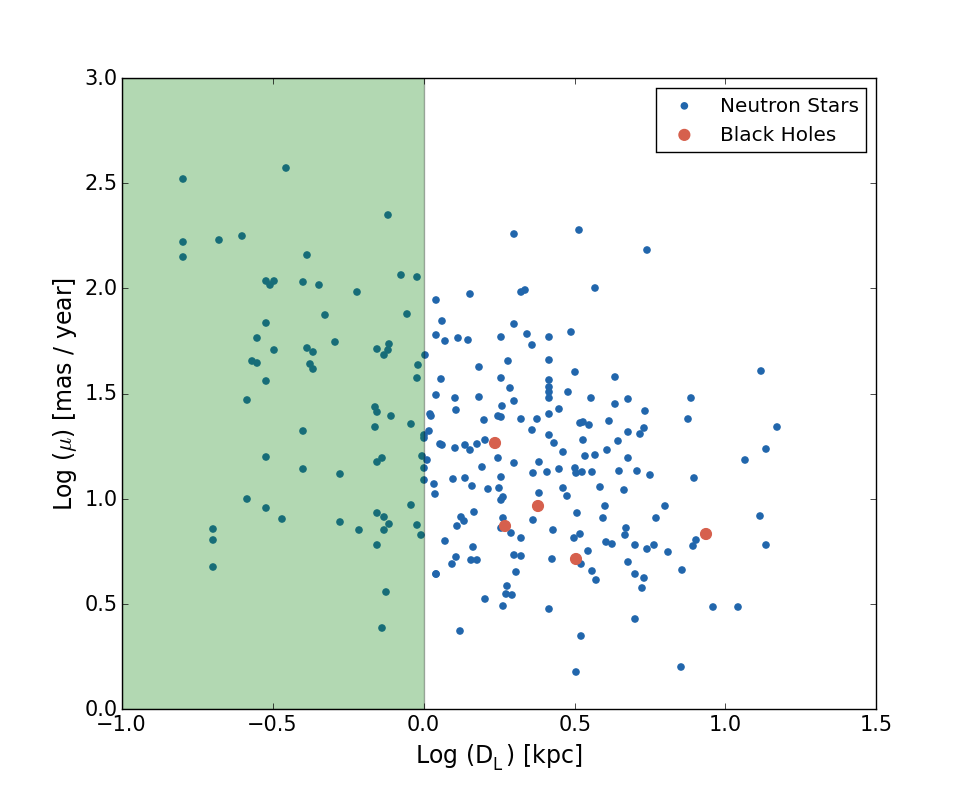
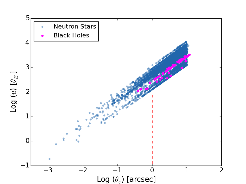
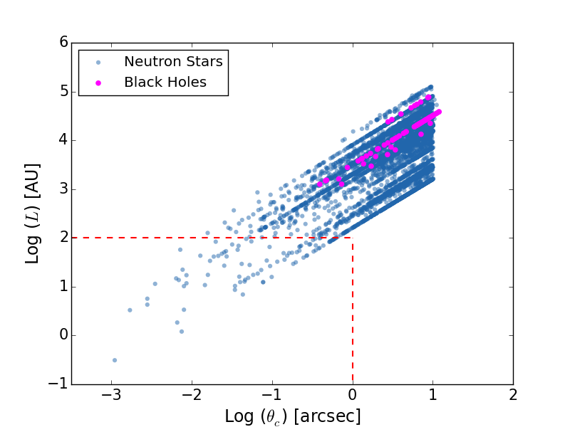
Fig. 1 is a log-log plot of proper motion versus distance for all the neutron stars and black holes we consider as potential lenses. These two are the most critical parameters for achieving a high microlensing rate per lens. Potential lenses located within a kpc will therefore dominate the rate of events that can be predicted. The green shaded region highlights all objects located within 1 kpc. One fourth of the potential lenses we consider are in this region, and 33 of them have proper motions $\mu\geq 40$ mas yr^-1; These neutron stars and black holes produce the highest average microlensing rate, per lens.

Table 3: Proper motion $\mu$, lens distance $D_{L}$, and Einstein angle $\theta_{E}$ for the five black holes in the BlackCat catalogue of Corral-Santana, J. M. et al. (2016) that happen to have measured proper motions.

Name	$\mu$	$D_{L}$	$\theta_{E}$	Detectability	Density	Rate
	mas yr-1	kpc	mas	Factor	per arcmin2	per Decade
Cyg X-1	7.43	1.86	7.54	25.13	38.52	3.01$\times 10^{-4}$
V404 Cyg	9.20	2.39	5.19	17.29	21.65	9.92$\times 10^{-5}$
GRO J1655-40	5.19	3.20	3.66	12.20	58.25	7.49$\times 10^{-5}$
GRS 1915+105	6.83	8.60	3.16	10.52	13.05	1.65$\times 10^{-5}$
XTE J1118+480	18.36	1.72	5.35	17.84	1.27	1.24$\times 10^{-5}$

Figure 1: Proper motions and distances for the neutron stars and black holes included in this study. Their proximity and generally higher proper motion means that these objects can generate lensing events at relatively high rates. Proper motions are available at this time for only five black hole systems; they are shown in red.

3.2 Catalogues of Background Sources

One reason that event prediction is now a practical endeavour is the availability of a variety of all-sky catalogues which can be used to map out background sources in the vicinity of known target lenses. For the present study, we utilized the catalogues listed in Table 4, which list sources detected at optical wavelengths and in the infrared.

The Gaia mission is of special importance to this study. First, Gaia has the highest astrometric precision of any all-sky survey to date, with the first data release (September 2016) providing positions of 1 billion nearby stars to $10$ mas precision (Gaia Collaboration et al., 2016a). The survey will have a magnitude limit of $20.5$ mag, and will eventually measure the positions of the brightest (dimmest) stars to about $5-10$ $\mu$as (a few hundred $\mu$as). Gaia will therefore discover many lensing events, among them events in which some of the compact objects we consider here serve as lenses.

The Sloan Digital Sky Survey has lower astrometric precision ($45$ mas RMS for each coordinate). It also has a fainter magnitude limit and can thus identify dimmer background sources. Unfortunately, SDSS has limited coverage at low galactic latitudes, where large surface densities can assure higher rates of lensing events.

With its sensitivity and high angular resolution, HST can provide a unique look at the background of a potential lens. Source extraction for many fields with HST images has been conducted and the results are listed in the The Hubble Source Catalog (HSC), which we have used. The HSC reaches the faintest magnitudes with relatively high astrometric precision, but it has very limited sky coverage.

The 2MASS catalogue is useful as an all-sky infrared catalogue, particularly when the potential lenses are compact objects. White dwarfs, for example, tend to be relatively blue, and are therefore dim in the infrared. Blending of light from the the lens is therefore less problematic than it can be in other cases.

These 4 catalogues complement each other. In addition, they have some stars in common, which allows cross-matching to establish a frame of reference that improves the precision of relative positions. In addition, the fact that the observations in the catalogues were generally taken at different times, provides additional constraints on the relative proper motions of the lens and background sources.

Table 4: List of catalogues used to supply background sources in the fields of the lens candidates.

Catalogue	Waveband	Magnitude Limit	Reference
2MASS	Infrared	J$\approx$16	Cutri et al. (2003)
Hubble Source Catalog (HSC)	Optical/Infrared	V$\approx$24	Whitmore et al. (2015)
Gaia first data release	Optical	V$\approx$20	Gaia Collaboration et al. (2016b)
SDSS	Optical	V$\approx$22	Ahn et al. (2012)

3.3 Background Source Densities

The 2MASS, SDSS, and Gaia catalogues are all available for query through the VizieR service. For each catalogue, we retrieved all sources located within 1 arcmin of the position of each of the the $2,536$ neutron stars listed in the ATNF, each of the $60$ black holes from the BlackCat catalogue, and each of the $35,246$ white dwarf candidates from the SUPERBLINK catalogue. We then calculated background source densities per square arcmin in the vicinity of each compact object by counting the number of sources within 1 arcmin of it, then dividing by the area ($\pi$ square arcminutes).

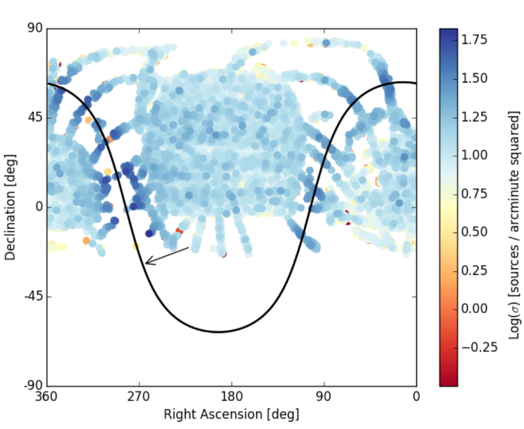
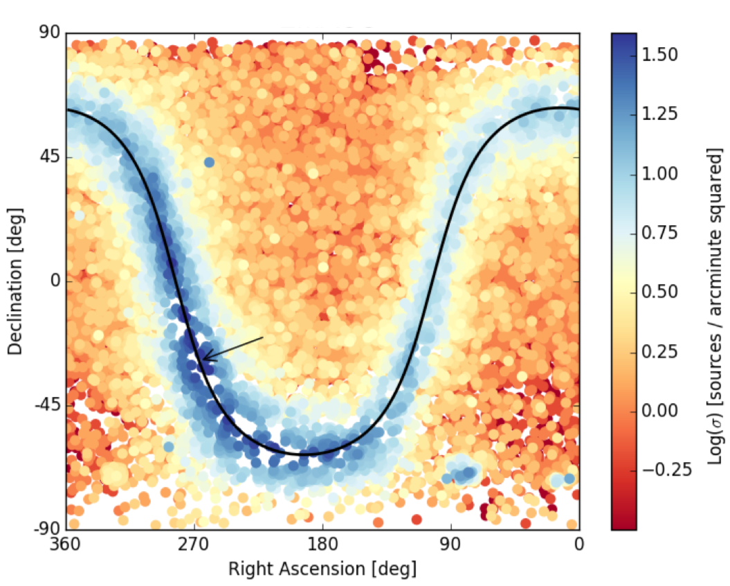
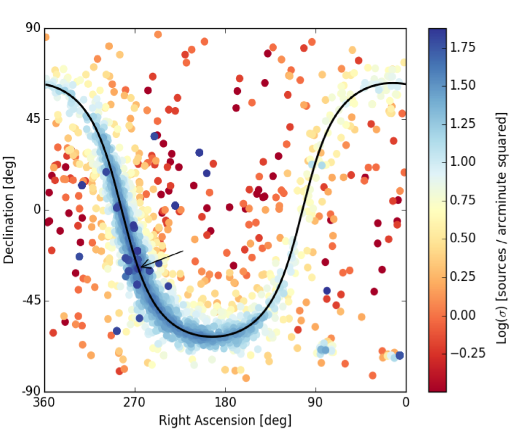
Fig. 2 shows the SDSS and 2MASS density maps for the white dwarfs and Fig. 3 shows the 2MASS background source density map for the neutron stars. As expected, the densest regions follow the line of the galactic plane, with some of the highest densities found near to the galactic bulge. Regions of high source density outside the Disk include the Magellanic Clouds and some globular clusters.

Figure 2: Density of background sources in the areas immediately surrounding the 35,246 white dwarfs considered in this study. Each coloured orb represents one of the white dwarfs, with the colour corresponding to the source field density. These two panels show the field density for sources listed in SDSS and 2MASS. The colour scales with the log of the local field density; note that the colour scale varies between plots. The densest regions appear along the black line that represents the galactic plane. The arrow in each map points to the location of the galactic center.

Figure 3: Density of background sources in the areas immediately surrounding the $2,544$ neutron stars considered in this study. Each coloured orb represents one of the neutron stars, with the colour corresponding to the source field density. The panel shown here maps the field density for sources listed in 2MASS. We expect neutron stars near the bulge to have the highest probability of generating microlensing events due to the large number of sources in this region.

We computed densities in background fields for the 26 neutron stars and 1 black hole with recorded proper motion that had been imaged by HST before early 2016. We also required that there be a corresponding source list in the HSC. We used the interactive viewer in the Hubble Legacy Archive. We calculated the field densities by counting all HSC-listed sources in those HST images, dividing by the coverage area of the particular imager that was used (WFPC2, ACS, or WFC3). In cases of observations with multiple overlapping fields, we counted only the sources within the borders of the field whose center was closest to the target. If the sources were extracted from a WFPC2 image, we also excluded sources from the PC chip. The resulting densities are shown in Table 5. As expected, source densities are systematically higher than those from the ground-based catalogues because of the fainter magnitude limit.

Table 5: Background source densities in the Hubble Source Catalog, for neutron stars that have been imaged with HST. The table also lists the ratio between the HSC source density and the values calculated from the other three catalogues (2MASS, SDSS, Gaia) to show the significant increase in background sources that can be achieved with deeper surveys.

Lens ID	HSC source density	$\epsilon_{SDSS}$	$\epsilon_{2MASS}$	$\epsilon_{Gaia}$
	arcmin-2
J0205+6449	110.01	2.93	16.46	5.57
J0437-4715	6.61	-	10.39	3.46
J534+2200	149.76	-	10.69	20.46
J0621+1002	96.0	-	15.87	8.38
J0633+1746	35.63	-	6.22	3.61
J0659+1414	50.56	2.48	13.24	8.36
J0821-4300	106.45	-	19.67	6.43
J0823+0159	10.67	0.88	8.38	4.79
J0835-4510	205.65	-	20.84	6.80
J1057-5226	128.0	-	14.36	6.09
J1455-3330	89.39	-	70.20	17.55
J1640+2224	25.17	2.26	39.54	9.89
J1713+0747	84.91	-	88.91	26.67
J1856-3754	199.04	-	26.05	16.90
J1857+0943	391.47	-	18.92	6.58
J1952+3252	583.04	-	26.17	9.49
J1959+2048	299.09	-	19.18	5.22
J2019+2425	138.24	-	18.10	4.34
J2033+1734	93.23	-	26.63	8.37
J2051-0827	23.68	-	14.88	9.30
J2145-0750	46.51	6.64	73.05	29.22
J2225+6535	54.40	-	11.39	5.70
Average $\epsilon$		3.04	25.87	10.14

Figure 4: HST WFPC2 image taken in the F675W filter on the 20^th June 2001. The bright companion of the black hole GRO J1655-40 can be seen near the center of the field. The sources circled are those found in the source catalogues we’ve used: HSC (pink), GSC2.3 (purple), Gaia (orange), 2MASS (green) and USNO-B1.0 (red). Many sources are visible in the image that have not been included in any of the source catalogues.

We note that source lists in the HSC are not necessarily complete. One example is shown in Fig. 4 which plots an observation of GRO J1655-40 with the WFPC2 on HST. The overlay of sources listed in the HSC clearly only flag the brightest objects in the field, missing the majority of the fainter sources, which tend to be $\sim 10$ times more numerous than those listed in the HSC. Because most of the unlisted stars are dimmer, approaches by a passing stellar remnant may have to be closer in order for an event to be detectable. Nevertheless, this suggests that the rate of microlensing events detectable through HST imaging may be several times higher that the rates predicted based on the HSC alone. It is also important that even background sources that are distant galaxies can be detectably lensed, but these are not included in the HSC.

Only a small fraction of the sky has been imaged by HST. Yet, since it can be a frontline tool for the prediction and observation of astrometric lensing events, it is useful to estimate the background densities that could be measured, were HST employed to image more fields containing stellar remnants. We have therefore considered fields for which we have computed background surface densities based on SDSS, 2MASS, and/or Gaia, and for which HST imaging is also available. In the latter case, we have used the HSC to compute the local source density. The specific fields we have studied in this way all contain the coordinates of a neutron star with known distance and proper motion. For each such field, we have $\sigma_{\rm HSC}$ from the HSC, and $\sigma_{\rm cat}$ from some other catalogue(s). We define the ratio $\epsilon=\frac{\sigma_{\rm HSC}}{\sigma_{\rm cat}}$. Average values $\epsilon$ for all fields are found to vary between $3-25$. This means that, by taking HST images of regions with potential lenses in the foreground, we can increase the rate at which we can observe lensing events by around an order of magnitude.

3.4 Microlensing Rates

We apply Equation 7 to calculate the average rate of microlensing events for each candidate lens, using the measured background source densities estimated above. We start by considering individual compact objects which, because some combination of proximity and high proper motion, may produce microlensing events at high average rates. Examples are shown in Tables 1, 2, and 3, for white dwarfs, neutron stars, and black holes respectively. Note that the rates are averages, based on the local background density.

To determine the time of the next event for any individual compact object, it is necessary to consider the positions of each nearby background source with respect to the path of the compact object. Nevertheless, this short list makes it clear that it is not difficult to identify individual white dwarfs that will produce events in the near future. For neutron stars and black holes, the rates are far smaller. Nevertheless, in §5 we will show through the study of a specific neutron star, that predictions may be possible for small numbers of neutron stars, and potentially for black holes as well.

We first calculate individual rates for the $35,246$ white dwarfs for each of the photometric catalogues, shown in Table 6. The top of Table 6 lists the rate per white dwarf per decade. The fourth column suggests that one would need to study the positions of approximately $1000$ white dwarfs in order to detect an event each decade. We note however, that these estimates are based on averaging white dwarfs that produce events several times per century with others that produce events at much lower rates. It is therefore possible to select a smaller subset of white dwarfs to ensure detecting one or more events per decade.

It is also important that large values of the detectability factor, ${\cal F}$, mean that the time interval during which astrometric shifts can be detected may be years or decades. If, therefore, we identify our computed rates with the numbers of events that will peak per year, the numbers that will be detectable each year are larger, because some detectable events will have peaked during previous decades and others will peak during future decades.

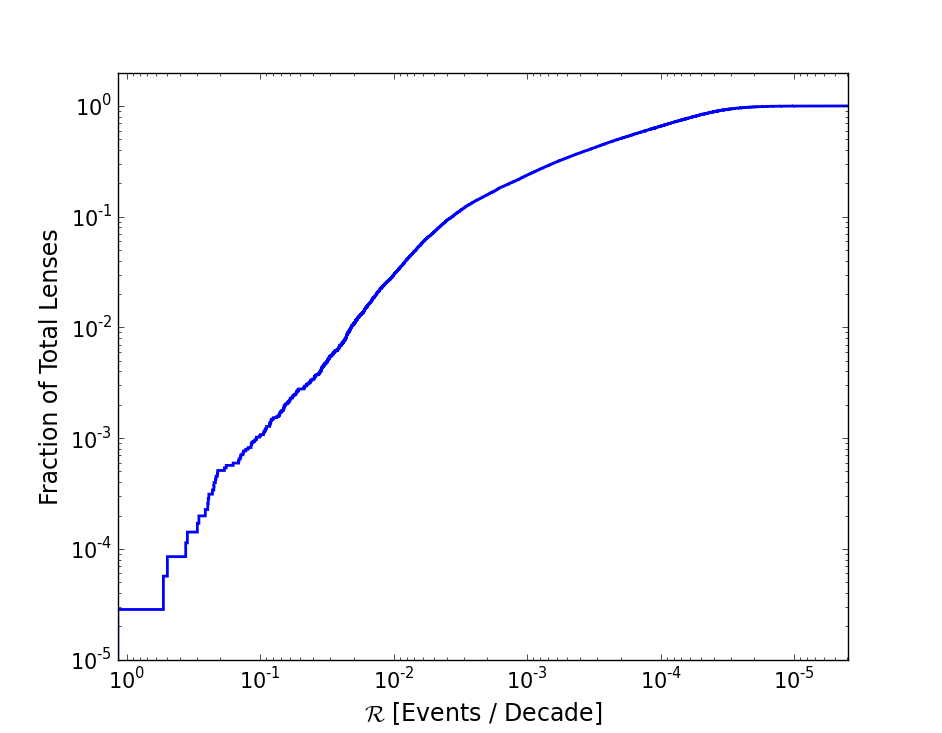
Fig. 5 shows two cumulative distribution plots, with the estimated event rate, $\cal{R}$, in a logarithmic scale on the x-axis. The rate values are those determined with background source densities measured from the Gaia catalogue. The top panel in the figure is for the white dwarfs which shows that $\sim$ $0.1$ per cent of the white dwarfs ($\sim$ $35$ lenses) are expected to produce events at a rate $>0.1$ events per decade. These white dwarfs are the most interesting to focus on because they have a good combination of high proper motions, high density background stellar fields, and are at relatively small distances from Earth.

In the bottom half of Table 6 the total combined rates for all of the white dwarfs we consider are listed. Even without the HST enhancement factor, and even before considering events that may peak during prior or subsequent decades, we expect $2-4$ dozen white-dwarf-generated astrometric events per decade. Note that these total combined rates refer only to the total set of white dwarfs that we have considered. By including known white dwarfs with smaller measured proper motions, the numbers would be significantly increased. Futhermore, ongoing studies, including those with Gaia, are adding to the list of white dwarfs with measured distances and proper motions.

We have carried out the same procedure for the $250$ neutron stars and $5$ black holes in our sample. We averaged the values to estimate an overall rate of microlensing events per lens. These rates are calculated separately for each photometric catalogue, and listed in Tables 7 and 8. The rates quoted in the top portions of the tables are expressed in microlensing events per compact object per decade. The numbers are roughly ten times smaller for neutron stars (relative to white dwarfs), because there are so few neutron stars with measured distances and proper motion, that the 3-dimensional density is small and most are at larger distances and have smaller proper motions than a large fraction of the white dwarfs in our sample. There is an additional factor-of-ten decline for black holes.

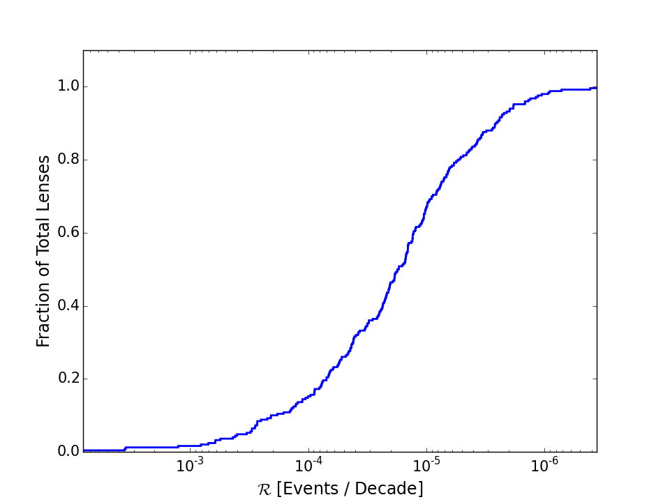
The bottom panel of Fig. 5 shows the cumulative distrubtion plot for the event rates of the neutron stars. It can be seen in the figure that the top $\sim$ $15$ per cent of the neutron stars are estimated to only produce $>10^{-4}$ events per decade. The message from these calculations is that we would need to identify more neutron stars and black holes and measure their distances and proper motions, in order to make event prediction a practical endeavour. In spite of this apparently grim prognosis, we will show in §5 that at least one neutron star has apparently generated events in the recent past. This demonstrates that fluctuations can play a role in increasing the local rate of events (as opposed to the long-term average). In addition, the existence of dim background stars that have not been catalogued in the HSC mean that our computed rates are too low. The example we present in §5 explicitly illustrates this point.

Despite the fainter magnitude limit of the SDSS, the event rate from this catalogue is comparable to the event rate for the 2MASS catalogue, and about an order of magnitude lower than for the Gaia catalogue. This is because of the patchy coverage of SDSS at low magnitude, which excludes the densest areas of the sky. This shows the need for deeper astrometric surveys at low galactic latitudes, which would significantly increase the potential for event prediction.

Figure 5: Cumulative distribution plots for the the event rate, $\cal{R}$, for the white dwarfs (Top) and neutron stars (Bottom) with measured distances and proper motions. Plotted on the horizontal axes is the logarithm to the base ten of the rate per decade calcualted using $\sigma$ from the Gaia catalogue.

Table 6: Estimated average event rates for the white dwarf candidates, calculated from the surface densities of the background regions of white dwarfs with measured proper motions. Top: the rate per compact object, averaging over all the white dwarfs in our sample. Bottom: the overall rate is the rate expected from all the white dwarfs in our sample combined.

Lens Category	Source	Lenses with Nearby	Rate per Compact	Enhanced Rate
	Catalogue	Background Sources	Object per Decade	(Rate x $\epsilon$)
White Dwarfs	SDSS	18,208	1.61 $\times 10^{-3}$	4.89 $\times 10^{-3}$
(35,246 objects)	2MASS	31,769	7.62 $\times 10^{-4}$	1.97 $\times 10^{-2}$
	Gaia	34,519	1.52 $\times 10^{-3}$	1.54 $\times 10^{-2}$
Lens Category	Source	Lenses with Nearby	Overall Rate	Enhanced Rate
	Catalogue	Background Sources	per Decade	(Rate x $\epsilon$)
White Dwarfs	SDSS	18,208	29.27	88.98
(35,246 objects)	2MASS	31,769	24.22	626.57
	Gaia	34,519	52.37	531.03

Table 7: Estimated theoretical event rates for the neutron star and lens candidates, calculated from areas that contain lenses with measured proper motions. The overall rate is the rate expected from all the lenses combined.

Lens Category	Source	Lenses with Nearby	Rate per Compact	Enhanced Rate
	Catalogue	Background Sources	Object per Decade	(Rate x $\epsilon$)
Neutron Stars	SDSS	54	1.01$\times 10^{-4}$	3.07$\times 10^{-4}$
(250 Objects)	2MASS	239	5.31$\times 10^{-5}$	1.37 $\times 10^{-3}$
	Gaia	249	1.36$\times 10^{-4}$	1.38$\times 10^{-3}$
Lens Category	Source	Lenses with Nearby	Overall Rate	Enhanced Rate
	Catalogue	Background Sources	per Decade	(Rate x $\epsilon$)
Neutron Stars	SDSS	54	5.43$\times 10^{-3}$	1.65$\times 10^{-2}$
(250 Objects)	2MASS	239	1.27$\times 10^{-2}$	3.29$\times 10^{-1}$
	Gaia	249	3.38$\times 10^{-2}$	3.43$\times 10^{-1}$

Table 8: Estimated theoretical event rates for the black hole lens candidates, calculated from areas that contain lenses with measured proper motions. The overall rate is the rate expected from all the lenses combined.

Lens Category	Source	Lenses with Nearby	Rate per Compact	Enhanced Rate
	Catalogue	Background Sources	Object per Decade	(Rate x $\epsilon$)
Black Holes	SDSS	1	4.03$\times 10^{-5}$	1.23$\times 10^{-4}$
(5 Objects)	2MASS	5	5.36$\times 10^{-5}$	1.39 $\times 10^{-3}$
	Gaia	5	1.01$\times 10^{-4}$	1.02$\times 10^{-3}$
Lens Category	Source	Lenses with Nearby	Overall Rate	Enhanced Rate
	Catalogue	Background Sources	per Decade	(Rate x $\epsilon$)
Black Holes	SDSS	1	4.03$\times 10^{-5}$	1.23$\times 10^{-4}$
(5 Objects)	2MASS	5	2.68$\times 10^{-4}$	6.93 $\times 10^{-3}$
	Gaia	5	5.04$\times 10^{-4}$	5.11$\times 10^{-3}$

4 Predicting Close Passages

In §3 we computed the average rate of events to be generated by each lens using the density, $\sigma$, of background stars. Typical densities are small enough that local fluctuations actually determine when the next detectable event will be generated by a specific foreground lens. For example, a potential lens producing a low average rate may happen to be close to a nearby star, and it may also be traveling toward the position of that star. Such a mass may therefore produce a detectable lensing event in the near future. In this section we therefore consider the individual position of each background star listed in each catalogue. Using the position of the foreground object as it was during a specific epoch, and its proper motion, we determine the distances and times of specific future close approaches it will make to background stars. This procedure identifies the potential lenses whose paths should be studied in the near future. It is the next step toward our ultimate goal of predicting specific lensing events to be generated by compact objects, and planning observations of the associated centroid shifts.

4.1 General Method and Caveats

We consider the sets of white dwarfs, neutron stars and black holes introduced in §3. For each nearby stellar remnant with known proper motion, we retrieve the positions of background field stars. Because future observations of astrometric events will likely be taken by HST or Gaia, we explore the close approaches between potential lenses and the stars listed in the HSC and in the Gaia catalogue. We focus on approaches that would cause centroid shifts $\delta(u)>0.3$ mas, a realistic limit for HST. We note, however, that Gaia can measure positions with higher precision, making it possible to detect events for more distant approaches and thereby increasing the event rate.

We then calculate the angular distances between the background sources and a straight line representing the extrapolated path of the stellar remnant over time. We flag any approaches that come close enough for a detectable lensing event to occur, and calculate both the time of closest approach and the angular separation at that time. If this procedure identifies one or more close approaches, parallax effects and the motion of the background star must also be computed and taken into account.

In practice, the calculations are affected by several sources of uncertainty: (1) uncertainties in the absolute positions of faint background sources; (2) uncertainties in the proper motions of the potential lenses, which can build to uncertainties of $\sim 1$ arcsec over a century; (3) the proper motions of typical field stars, which may be a few mas yr^-1 due to random motions or to galactic differential rotation; these can add uncertainties of $\sim 1$ arcsec over a century. These three factors contribute to the uncertainty in such a way that it accumulates over time, making reliable prediction of future events strongly dependent on the predicted time of closest approach: the sooner the event occurs, the greater the reliability.

On the other hand, even more distant approaches may have the potential to produce microlensing events. For example, astrometric effects can be detected out to $\theta_{E}^{2}/\delta\phi$, which can be larger than an arcsec. In addition, the planetary system of a compact object may include wide-orbit planets, possibly even to the edge of the Oort Cloud. Oort Cloud radii are in the range $10^{4}\--10^{5}$ AU, and the distance to nearby stellar remnants are in the range from about 10 pc to a few kpc. Thus, wide-orbit planets could be $1\--1000$ arcsec from the stellar remnant they orbit. Note that, if we consider lensing by objects in the most distant reaches of possible Oort Clouds, then the positions of large numbers of background stars would need to be monitored. Here we will specifically consider only close approaches between the compact object itself and a background star.

4.2 Computing the Path of the Lens

For every object with a measured proper motion, $\mu$, we use the components of the proper motion in right ascension and declination, $\mu_{\alpha}$ and $\mu_{\delta}$ multiplied by $(t-t_{epoch})$.

$$\alpha(t)=\alpha_{epoch}+\mu_{\alpha}(t-t_{epoch}),\quad\delta(t)=\delta_{epoch}+\mu_{\delta}(t-t_{epoch})$$ (8)

We have computed the paths of all white dwarfs from the year 2020 through the year 2035, to allow us to identify any events of the recent past (which may be detectable, e.g. in archived HST data) as well as within the coming $\sim 18$ years Because the numbers of white dwarf we are considering is large, we will derive an estimate of the average event rate, which can be checked against the rates computed in §3. Because there are many fewer neutron stars and black holes, we have projected their paths over a baseline that is $\sim 200$ times longer, extending 2000 years into both the past and future. We note that some events that occurred over historical times may have produced high enough magnifications to have been detected as naked eye brightening of background stars. For such possible close approaches, historical records, including optical plates from the 1800s, can be investigated for strong lensing events.

For each compact object, we retrieve from the relevant catalogue the coordinates and magnitudes of all the sources located within 10 arcsec of the line segment defining the path of the lens.

4.3 Measured Approaches and Event Rates for White Dwarfs

Our simulation of the paths of the white dwarfs from SUPERBLINK during the interval 2016$\--$2035 found that every white dwarf will travel through a region containing background stars listed in the Gaia catalogue, and that $358$ approaches will produce detectable astrometric lensing events. This corresponds to an event rate of approximately 36 per decade, somewhat lower than the average listed in Table 6. Roughly 46 per cent of these approaches will be closer than $10\,\theta_{E},$ and 13 white dwarfs will come within $\theta_{E}$ of a Gaia-listed star. High-resolution images of these $13$ regions can determine whether the passages will actually be this close. If so, detectable photometric effects are expected. Only $62$ ($0.18$ per cent) of the white dwarfs will follow paths in regions containing sources listed in the HSC. We found $31$ close approaches between white dwarfs and HSC sources.

4.4 Measured Approaches and Event Rates for Neutron Stars and Black Holes

The HSC includes observations covering the fields of 26 of the neutron stars. Over the time span under consideration ($\pm 2000$ years), we identify 289 approaches where any one of these 26 neutron stars with come within $1$ arcsec of a background source. Of these, we find $15$ events with causing centroid shifts $\delta(u)>0.3$ mas. This suggests a rate of $\approx 1.5\times 10^{-3}$ per star per decade.

The Gaia catalogue lists sources along the paths of all $249$ neutron stars in our sample. Over the time span under consideration ($\pm 2000$ years), we identify 338 approaches where any one of these 250 neutron stars come within 1arcsec of a background source. Of these, we find $19$ events with centroid shifts $\delta(u)>0.3$ mas. This suggests a rate of $\approx 1.9\times 10^{-4}$ per star per decade. The lower rate of occurrence reflects the brighter magnitude limit of the Gaia catalogue (V$\lesssim$20) compared to that of the HSC (V$\lesssim$25).

All the approaches from the analysis for the black holes and neutron stars are plotted in Fig. 6. The top and bottom plots show the approach distances in arcsec against the impact parameter and distance $L$ (units of AU) respectively. The dashed red lines border the zones of the most interesting approaches. Approaches that come within $u=100~{}\theta_{E}$ are potentially capable of producing measurable lensing effects. The approaches with minimum distances less than $L=100$ AU provide good opportunities to investigate the existence of close orbiting exoplanets.

Figure 6: Top: log of the distance of closest approach in units of the Einstein angle plotted against the log of the impact parameter in arcsec, for all the potential lens/source encounters in our sample of neutron stars and black holes. Each oblique line artefact corresponds to a specific neutron star or black hole lens, because the Einstein angle and impact parameter are both correlated, and their ratio corresponds to our distance to the lens. Events for which astrometric shifts can be detected are those with distances of closest approach less than $100~{}\theta_{E}$ (horizontal dashed line) which happen only in events where the impact parameter is less than 1arcsec (vertical dashed line). Bottom: physical distance of closest approach, in AU, plotted against the log of the impact parameter in arcsec, for the same subset.

We find that none of the approaches between the black holes and background sources produced a maximum centroid shift $>0.3$ mas. Over the $4,000$ year time period, $9$ approaches came within $1$ arcsec, none of which are estimated to be in the detectable range. These rates were to be expected, as $\ll 1$ event per decade was predicted in §3, even when multiplying by the HSC density factor $\epsilon$. With so few objects in this sample, finding frequent events was unlikely. All of these objects are several kpc away and have low proper motions ($\sim 10$ mas yr^-1) so they will only cover a small area of the sky, even over long time periods.

Figure 7: A plot showing the log of the centroid shift at the closest approach for every passage made by neutron stars and black holes to nearby background sources. The two red lines show the detectability limits discussed in §1. The hashed region delineates the 2000$\--$2050 time period.

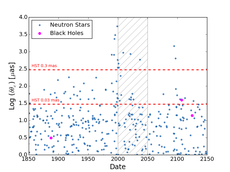
The close approaches predicted by our simulation are based on a detectability cut-off of $\delta(u)>0.3$ mas. However if future imaging techniques are improved (e.g. Riess et al. (2014)) then more approaches will fall into the detectable category. This is shown in Fig. 7 which plots the log of the maximum centroid shift against the time of closest approach. The two red lines correspond to detectability limits of $0.3$ mas and $0.03$ mas. From this plot we can see that many more approaches would be detectable if astrometric precisions of $x=0.03$ mas are attainable.

5 Prediction of Specific Events

To predict a specific event, we need to estimate the distance of closest approach in units of $\theta_{E}.$ Using images of the region, we can determine the distance of closest approach in milliarcsec. To express the distance in units of $\theta_{E}$, we need the distance, $D_{L}$ to the lens and an estimate of its mass. As before we use $M_{L}=1.4\,M_{\odot}$ for neutron stars and $M_{L}=0.6\,M_{\odot}$ for white dwarfs. If the lens produces an event that we can detect and study, we will measure its mass to high precision.

In principle, event prediction requires at least two high-resolution images, to allow us to locate the potential lens relative to the positions of background stars, and to measure relative motions. We note, however, that in some cases we may find in a single high-resolution image that the lens is already close enough to a background star to be causing a detectable astrometric shift. When this occurs, follow-up images (which may be taken several times over an interval of months or years) can track the shift; a subsequent image can determine the unshifted source position.

5.1 RX J1856.5-3754

The neutron star predicted to produce lensing events at one of the highest rate is RX J1856.5-3754. Known as a member of the Magnificent Seven (Haberl, 2007), RX J1856.5-3754 was one of the first isolated neutron stars discovered by the ROSAT telescope. RX J1856.5-3754 has been imaged multiple times by HST, making it an ideal candidate for detailed analysis. Its position, proper motion and parallax have been measured on several occasions (Walter, 2001; Walter & Lattimer, 2002; Walter et al., 2010). Using these measurements, we take $D_{L}=123\pm 15$ pc, and parallax $\pi=8.2\pm 0.2$ mas. We then calculate the Einstein angle (with $M_{L}=1.4\,M_{\odot}$) to be $\theta_{E}=9.02\pm 0.61$ mas.

Figure 8: Two images of RX J1856.5-3754 taken by HST’s WFPC2 camera in the F606W filter at different epochs. The two dashed black lines run parallel to RX J1856.5-3754’s projected path. Top: 6^th October 1996, Bottom: 24^th March 2001.

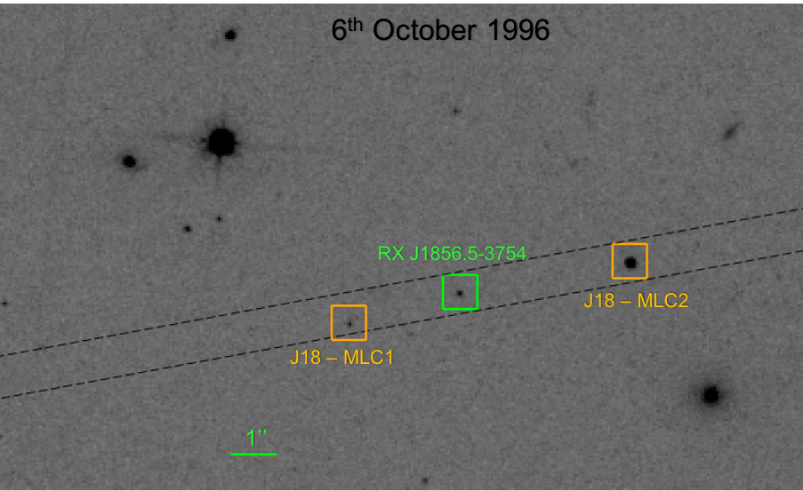
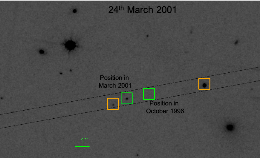
We retrieved two HST images of RX J1856.5-3754 from the HLA (epochs: 1996, 2001). They were taken by the PC1 chip of the WFPC2 camera with the F606W filter (wide V band). The images were uploaded to DS9 and the neutron star’s path overlaid (Fig. 8). It became apparent that two lensing events could have occurred in the past. For convenience we will refer to the two relevant background sources as J18-MLC1 and J18-MLC2; these are stars $\#$115 and $\#$23 in Walter (2001). J18-MLC1 does not appear in any source catalogue. Note that this is an example (like the one shown in Fig. 4) in which non-catalogued sources on the images can only be identified through visual examination.

RX J1856.5-3754’s proper motion is noticeable when comparing the two images. In contrast, there is no observable change in position for J18-MLC1 between the two images, suggesting a low proper motion, in agreement with Kaplan et al. (2002). J18-MLC2’s motion is much more prominent and has been measured by Walter et al. (2010). The motion due to of RX J1856.5-3754’s parallax would be a third of the size of a pixel in this image.

We computed the distances and times of closest approach. We take the starting positions of the lens and both sources from the 1996 image. By assuming that the uncertainties in position are the same for all the objects in the image, we have considered the relative positional errors to be negligible. We computed the closest distance of approach, $\delta\phi_{c}$, of RX J1856.5-3754 to J18-MLC1 to be $\delta\phi_{c}=194.94\pm 2$ mas, occurring on 25th April 2004. This estimate does not agree with the prediction made by Paczynski (2001), which estimated a closest approach to occur in June 2003, at a separation of $\sim 300$ mas. However Kaplan et al. (2002) revised this prediction and claimed an approach of distance $200$ mas in April 2004. This result agrees with our estimated prediction. We find the approach to be closer when taking J18-MLC1’s proper motion into account: $\delta\phi_{c}=167.78$ mas; the new time of approach is three days later. An approach of this distance would shift J18-MLC1’s centroid position by $\sim 0.48\pm 0.07$ mas, which is potentially detectable. Eight images were taken in the F475W filter with HST’s ACS/HRC camera during 2002$\--$2004. It is difficult to locate the source in the images but the observation taken in May 2004 appears to show RX J1856.5-3754 very close to J18-MLC1.

Figure 9: Predicted microlensing centroid shifts of the background sources J18-MLC1 and J18-MLC2, from a close passage of RX J1856.5-3754. The two red cut-off lines at $0.3$ and $0.03$ mas are the limits of possible detectability suggested by Bellini et al. (2011) and Riess et al. (2014) respectively. The close approach distances would cause detectable centroid shifts in both sources.

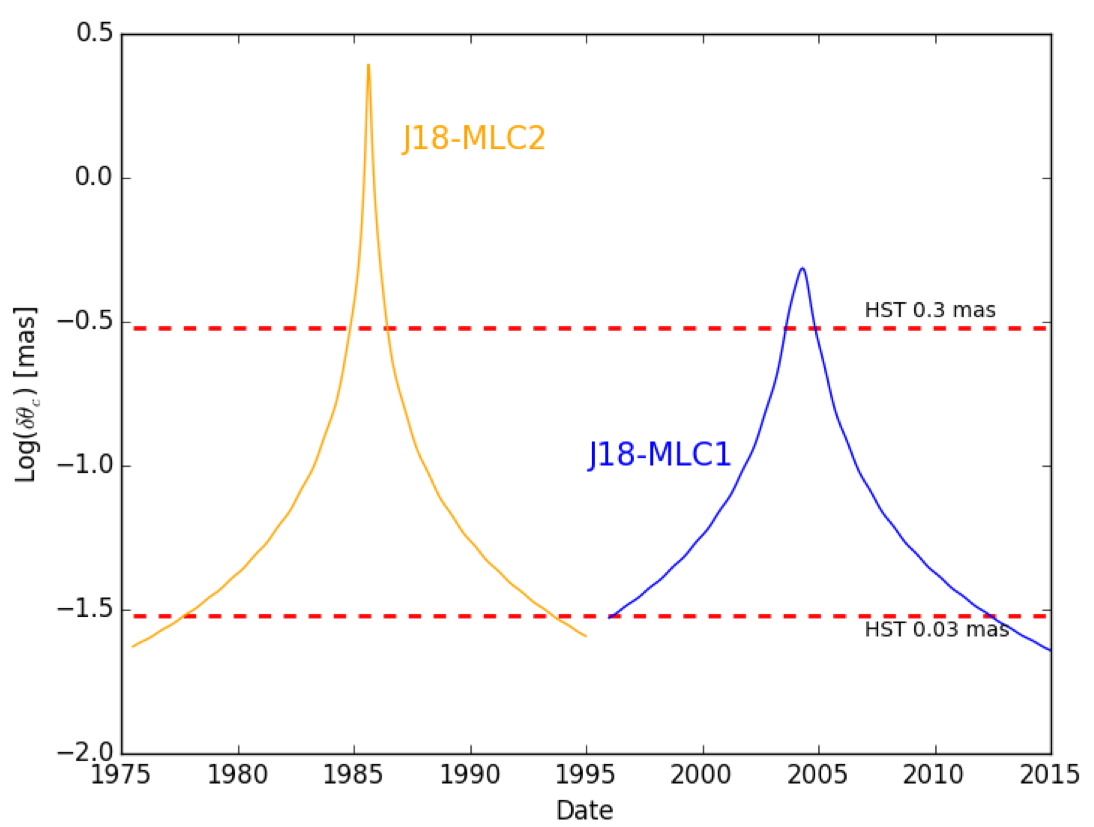
We also find that J18-MLC2 was lensed in August 1985. The closest approach distance, $\delta\phi_{c}=33.23\pm 4$, mas would have produced a detectable astrometric shift of $2.45\pm 0.7$ mas, and a small photometric effect ($\sim 1$ per cent) as well.

We note that the durations of detectable events are determined by the detectability limit. We consider that the start (end) of an event occurs when the size of the centroid shift is greater (less) than the specified detectability limit. Fig. 9 shows that for a $0.3$ mas cut-off, the predicted events would be detectable for $\sim~{}1$ year. If smaller shifts of $0.03$ mas were detectable, then approaches as close as these would produce events observable for time intervals on the order of decades.

5.2 PM I12506+4110E

The white dwarf PM I12506+4110E is one of 62 white dwarfs for which we had HSC source lists and identified stars lying within $10$ arcsec of its path. Because our simulation registered a close approach distance of $60$ mas to a background HSC source, we analysed the corresponding HST images. The white dwarf was imaged during 2005 in two filters: the F555W and F435W filters on the ACS/WFC camera. In the image we found a second star near the white dwarf’s path. Neither of the stars that will be approached by the white dwarf are listed in catalogues covered by the VizieR service.

Figure 10: F555W HST image from the ACS/WFC camera taken in 2005 of the white dwarf PM I12506+4110E. The lens’s path passes directly between two background sources: PM12-MLC1 and PM12-MLC2. Top: shows the image with the HSC sources positions (pink) and position of the lens from SUPERBLINK (green) overlaid. The black hashed line shows the projected path of the lens originating for the SUPERBLINK position. Bottom: The source and lens positions have been calibrated by addition of an average shift. There are now two black lines representing the projected path, one is for the lens’s position from SUPERBLINK, the other from the HSC position. We use the HSC position to calculate the close approaches.

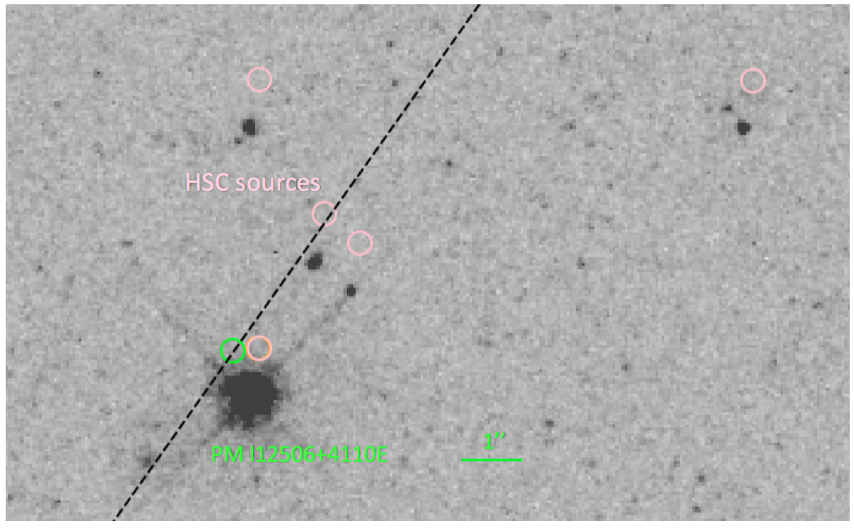
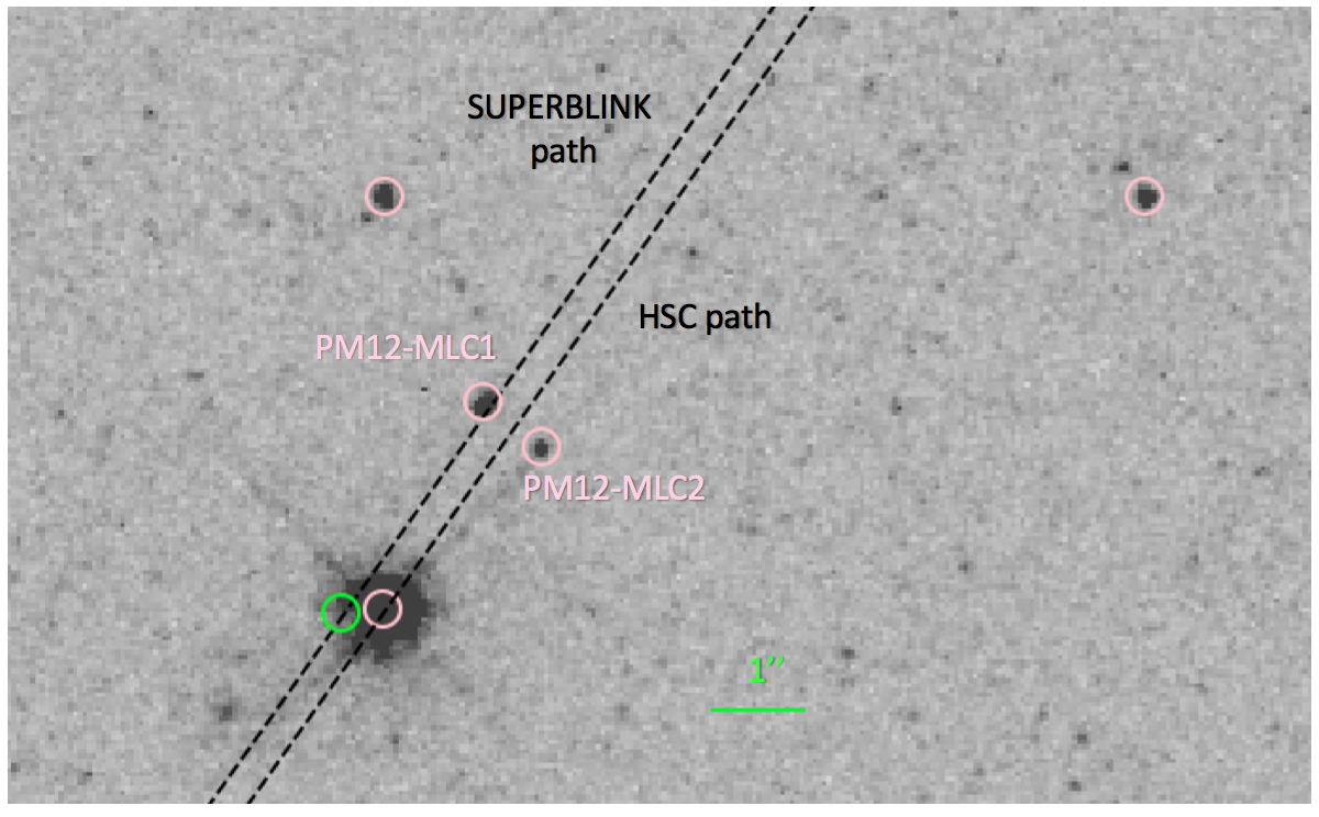
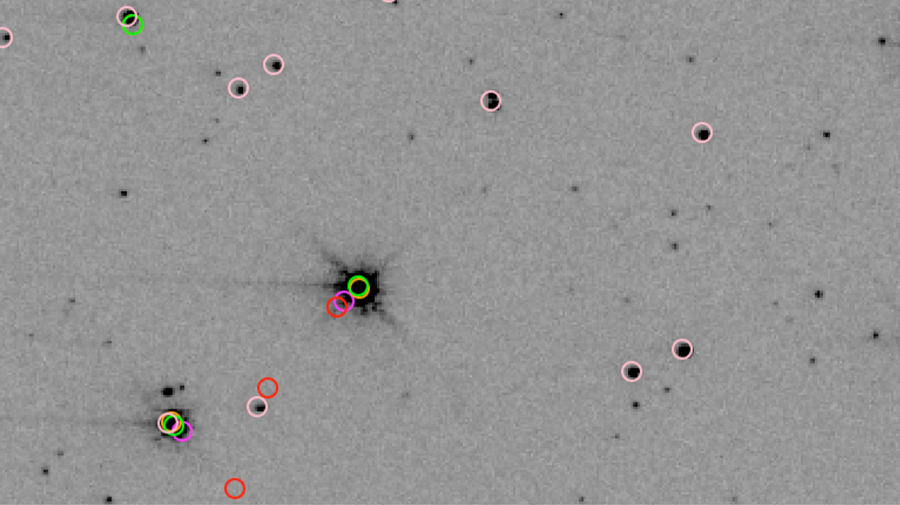
Fig. 10 shows the same image in both panels. The top panel shows the overlaid source positions from HSC (pink): one of these is PM I12506+4110E. The green circle is the position of the lens as computed from information in the SUPERBLINK catalogue. We made astrometric corrections to the image to produce the bottom panel of the Figure. The average shift between the HSC quoted positions and the positions on the image was calculated. Because we focus on this small area of the image, we used only the sources near the lens path to calculate the average shift. We applied the average shift to the HSC source positions. Even after this process was implemented, the white dwarf position derived from the SUPERBLINK catalogue is offset compared to the position of the white dwarf in the image. The paths based on both the SUPERBLINK and HSC positions have been plotted in the lower panel. The discrepancy is likely due to the position uncertainty from the SUPERBLINK catalogue. We use the path projected from the HSC position to make the event prediction.

We refer to the two background sources as PM12-MLC1 and PM12-MLC2. Using the proper motion provided by SUPERBLINK and the position of the lens from the HSC, we project the path of PM I12506+4110E. This path passes directly between the two sources. We predict approaches of $402.71$ mas to PM12-MLC1 and $346.23$ mas to PM12-MLC2 occurring in 2042 and 2044 respectively. Neither would produce a centroid shift $>0.3$ mas. With maximum uncertainties of $7$ mas yr^-1 on the proper motions (Lépine & Shara, 2005), over time, the path may diverge from the one we have projected. All possible paths of the lens will exist inside a cone with sides relating to the paths calculated with these maximum uncertainties. A path along one of these sides will come within $u\sim 9~{}\theta_{E}$ of PM12-MLC1, whereas a path along the other side will approach PM12-MLC2 at a distance of $u\sim 6~{}\theta_{E}$. Both of these approaches would produce centroid shifts of less than $1$ mas but greater than $0.3$ mas. This is an interesting case as uncertainties in the path provide a chance for PM I12506+4110E to pass close to one of the sources. Further imaging of this white dwarf will allow for improvements to the accuracy of our prediction. More observations will also be required to check for any proper motion in the two background sources.

6 Conclusions

We have demonstrated that the prediction of lensing events is a practical idea. The existence of deep catalogues of background objects is making work along these lines ever more practical. We applied these ideas to stellar remnants because of the importance of measuring their masses, a task to which gravitational microlensing is well suited. In addition, stellar remnants tend to be dim, making it easier to discern the changes wrought by lensing in the positions and brightness of background stars.

We find that the detection of lensing events due to white dwarfs can certainly be observed during the next decade by both Gaia and HST (Sahu et al., 2017). Photometric events will occur, but to detect them will require observations of the positions of hundreds to thousands of far-flung white dwarfs. As we learn the positions, distances to, and proper motions of larger numbers of white dwarfs through the completion of surveys such as Gaia and through ongoing and new wide-field surveys, the situation will continue to improve.

For neutron stars and black holes, the regular and systematic prediction of lensing events will be more challenging. The known populations are too small, and we do not have measured proper motions and/or distances even for the majority of the known systems. As new discoveries increase the known populations and as distance measurements and determinations of proper motions are made, the prospects for prediction will improve. Despite the low rate, we have found that at least one neutron star came close to producing detectable events in the recent past. This indicates the value of high-resolution imaging for compact objects that happen to be moving in front of dense stellar fields.

Within the next several years, the measurements of white dwarf masses seems poised to become a possible enterprise that will open a new window to the study of compact objects (Sahu et al., 2017). The discovery of planets orbiting compact objects will be an additional benefit of these studies.

References

- Abbott et al. (2016) Abbott B. P., et al., 2016, Phys. Rev. Lett., 116, 061102
- Ahn et al. (2012) Ahn C. P., et al., 2012, ApJS, 203, 21
- Backer et al. (1993) Backer D. C., Foster R. S., Sallmen S., 1993, Nature, 365, 817
- Bellini et al. (2011) Bellini A., Anderson J., Bedin L. R., 2011, PASP, 123, 622
- Borucki (2016) Borucki W. J., 2016, Reports on Progress in Physics, 79, 036901
- Corral-Santana, J. M. et al. (2016) Corral-Santana, J. M. Casares, J. Muñoz-Darias, T. Bauer, F. E. Martínez-Pais, I. G. Russell, D. M. 2016, A&A, 587, A61
- Cutri et al. (2003) Cutri R. M., et al., 2003, 2MASS All Sky Catalog of point sources.
- Di Stefano (2008) Di Stefano R., 2008, The Astrophysical Journal, 684, 59
- Di Stefano (2012) Di Stefano R., 2012, The Astrophysical Journal, 752, 105
- Di Stefano & Scalzo (1999) Di Stefano R., Scalzo R. A., 1999, The Astrophysical Journal, 512, 579
- Di Stefano et al. (2010) Di Stefano R., Howell S. B., Kawaler S. D., 2010, The Astrophysical Journal, 712, 142
- Di Stefano et al. (2013) Di Stefano R., Matthews J., Lépine S., 2013, ApJ, 771, 79
- Dominik & Sahu (2000) Dominik M., Sahu K. C., 2000, ApJ, 534, 213
- Falcon et al. (2012) Falcon R. E., Winget D. E., Montgomery M. H., Williams K. A., 2012, The Astrophysical Journal, 757, 116
- Gaia Collaboration et al. (2016a) Gaia Collaboration et al., 2016a, A&A, 595, A2
- Gaia Collaboration et al. (2016b) Gaia Collaboration et al., 2016b, A&A, 595, A2
- Gould & Loeb (1992) Gould A., Loeb A., 1992, ApJ, 396, 104
- Haberl (2007) Haberl F., 2007, Ap&SS, 308, 181
- Kaplan et al. (2002) Kaplan D. L., van Kerkwijk M. H., Anderson J., 2002, ApJ, 571, 447
- Lépine & Di Stefano (2012) Lépine S., Di Stefano R., 2012, ApJ, 749, L6
- Lépine & Shara (2005) Lépine S., Shara M. M., 2005, AJ, 129, 1483
- Limoges et al. (2013) Limoges M.-M., Lépine S., Bergeron P., 2013, The Astronomical Journal, 145, 136
- Manchester et al. (2005) Manchester R. N., Hobbs G. B., Teoh A., Hobbs M., 2005, VizieR Online Data Catalog, 7245
- Mao & Paczynski (1991) Mao S., Paczynski B., 1991, ApJ, 374, L37
- Miller-Jones (2014) Miller-Jones J. C. A., 2014, Publ. Astron. Soc. Australia, 31, e016
- Paczynski (1986) Paczynski B., 1986, ApJ, 304, 1
- Paczynski (2001) Paczynski B., 2001, ArXiv Astrophysics e-prints,
- Ricker et al. (2014) Ricker G. R., Vanderspek R. K., Latham D. W., Winn J. N., 2014, in American Astronomical Society Meeting Abstracts #224. p. 113.02
- Riess et al. (2014) Riess A. G., Casertano S., Anderson J., Mackenty J., Filippenko A. V., 2014, Astrophys. J., 785, 161
- Sahu et al. (2017) Sahu K. C., et al., 2017, in American Astronomical Society Meeting Abstracts. p. 315.13
- Walter (2001) Walter F. M., 2001, ApJ, 549, 433
- Walter & Lattimer (2002) Walter F. M., Lattimer J. M., 2002, ApJ, 576, L145
- Walter et al. (2010) Walter F. M., Eisenbeiß T., Lattimer J. M., Kim B., Hambaryan V., Neuhäuser R., 2010, ApJ, 724, 669
- Whitmore et al. (2015) Whitmore B. C., et al., 2015, in American Astronomical Society Meeting Abstracts. p. 332.05
- Wolszczan & Frail (1992) Wolszczan A., Frail D. A., 1992, Nature, 355, 145