An accurate scheme to calculate the interatomic
Dzyaloshinskii-Moriya interaction parameters

Abstract

An new and accurate scheme to calculate the interatomic Dzyaloshinskii-Moriya interaction (DMI) parameters is presented, which is based on the fully relativistic Korringa-Kohn-Rostoker Green function (KKR-GF) technique. Corresponding numerical results are compared with those obtained using other schemes reported in the literature. The differences found can be attributed primarily to the different reference states used in the various approaches. In addition an expression for the DMI parameters formulated for a micromagnetic model Hamiltonian is presented that provides a connection to the DMI parameters calculated for atomistic Hamiltonians. This formulation also allows the discussion of the DMI in terms of specific features of the electronic band structure.

I Introduction

Recent investigations on the influence of spin-orbit coupling (SOC) on the magnetic and transport properties of solids open the way for an efficient tuning of these properties concerning their application in various types of electronic devices based on new technologies. This concerns in particular new phenomena associated with a chiral magnetic texture, as for example skyrmions Bogdanov and Hubert (1994); Roszler et al. (2006) with the related topological and anomalous Hall effects Schulz et al. (2012); Neubauer et al. (2009) or chiral magnetic soliton lattices Togawa et al. (2012) with corresponding magneto-resistance phenomena Togawa et al. (2013). In fact, it is the SOC induced anisotropic Dzyaloshinskii-Moriya exchange interaction (DMI) that is responsible for the creation of such non-trivial magnetic textures in non-centrosymmetric systems. As in many other fields of material science the search for materials with corresponding favorable isotropic and anisotropic exchange coupling parameters can be substantially supported by first-principles investigations. Actually, several schemes to calculate the DMI parameters of a solid have been suggested with their explicit formulation depending on the underlying electronic structure method.

A rather flexible approach to calculate the exchange coupling parameters is based on the Korringa-Kohn-Rostoker Green function (KKR-GF) technique in its multiple scattering formulation. In fact two such schemes, scheme I Udvardi et al. (2003) and scheme II Ebert and Mankovsky (2009), based on the magnetic force theorem have been reported that can be seen as a relativistic generalization of the so-called Lichtenstein formula Liechtenstein et al. (1987) giving this way not only access to the isotropic exchange coupling parameter but to the exchange coupling tensor $\underline{J}_{ij}$. The components of the corresponding DMI vector $\vec{D}$ are determined by the anti-symmetric part of this tensor by a linear combination of the off-diagonal elements of $\underline{J}_{ij}$ (see below).

The mentioned KKR-GF based approaches allow a direct calculation of the exchange coupling tensor $\underline{J}_{ij}$ in real space with its elements given by the variation of single particle energy caused by an infinitesimal rotation of two magnetic moments $\vec{m}_{i}$ and $\vec{m}_{j}$ on the atomic sites $i$ and $j$, respectively. An alternative approach suggested in the literature is focused on the relevant parameters of micromagnetic models, i.e. the exchange stiffness $A$ and the DMI vector $\vec{D}$ Heide et al. (2008, 2009), that are obtained by fitting the spin-wave dispersion curve $\omega(\vec{q})$ calculated from first-principles using expressions based on these model parameters. A rather elegant way for the calculation of the micromagnetic DMI vector was suggested recently by Freimuth et al. Freimuth et al. (2014); Koretsune et al. (2015) exploiting a property of the spin wave spectra of non-centrosymmetric systems. While the corresponding spectra of centrosymmetric systems have a parabolic like dispersion around their minimum at the $\Gamma$ point ($\vec{q}=0$), the minimum moves away from the $\Gamma$ point for non-centrosymmetric systems due to the DMI with the dispersion at $\vec{q}=0$ becoming non-zero. This feature can be used to map the calculated electronic energy connected with a spin spiral configuration in the system to the microscopic Heisenberg model Hamiltonian, giving this way access to the DMI parameters Freimuth et al. (2014).

Starting from the scheme of Freimuth et al. Freimuth et al. (2014), a new scheme (scheme III) to calculate the DMI parameters for any pair of atoms is suggested here that is based on the KKR-GF method. As it will be demonstrated, the advantage of this approach is that it allows for any orientation of the magnetization the simultaneous calculation of the two components of the DMI vector perpendicular to the magnetization. These are the only components of $\vec{D}$ which can be determined as the magnetic moments have only two possible degrees of freedom to deviate from the magnetization direction. This implies also that the component of the DMI vector along the magnetization direction is not defined. The approach to be presented allows also a KKR-GF based formulation for the micromagnetic DMI, permitting a comparison of the DMI vectors formulated within two different approaches, but calculated using the same electronic structure method.

II Theoretical formulation

II.1 Hamiltonians

In order to derive an expression for the interatomic DMI vector $\vec{D}_{ij}$ we start from a fully relativistic description of the electronic structure of a magnetic solid on the basis of the Dirac Hamiltonian

$${\cal H}_{\rm D} = -ic\vec{\alpha}\cdot\vec{\nabla}+\frac{1}{2}\,c^{2}(\beta-1)$$ (1)

$$\qquad+\bar{V}(\vec{r})+\beta\,\vec{\sigma}\cdot\vec{B}(\vec{r})+e\vec{\alpha}\cdot\vec{A}(\vec{r})\;,$$

that is setup in the framework of relativistic spin density functional theory Engel and Dreizler (2011). Accordingly, ${\alpha}_{i}$ and $\beta$ are the standard Dirac matrices Rose (1961) while $\bar{V}(\vec{r})$ and $\vec{B}(\vec{r})$ are the spin independent and dependent parts of the electronic potential.

When adopting a simplified atomistic microscopic model approach, an expression for the exchange coupling tensor $\underline{J}_{ij}$ of the generalized Heisenberg Hamiltonian

$${\cal H}_{\rm H} = \sum_{ij}\hat{m}_{i}\,\underline{J}_{ij}\,\hat{m}_{j}$$ (2)

can be derived by mapping the magnetic energy obtained within electronic structure calculations based on Eq. (1) to the energy corresponding to this model Hamiltonian. Here, we focus on the contribution

$${\cal H}_{\rm DM} = \sum_{ij}\vec{D}_{ij}\cdot(\hat{m}_{i}\times\hat{m}_{j})$$ (3)

connected with the DMI between the magnetic moments $\vec{m}_{i}$ and $\vec{m}_{j}$, that is determined by the DMI vector $\vec{D}_{ij}=(D^{x}_{ij},D^{y}_{ij},D^{z}_{ij})$ with

$$D^{\gamma}_{ij} = \epsilon^{\alpha\beta\gamma}\frac{J^{\alpha\beta}_{ij}-J^{\beta\alpha}_{ij}}{2}\;.$$ (4)

In the micromagnetic approach, the magnetic state is characterized by the free energy density (omitting the magnetic anisotropy term)

$$F(\vec{r}) = \sum_{\mu,\nu}A^{\nu}\left(\frac{\partial m_{\mu}}{\partial r_{\nu}}\right)^{2}+\sum_{\mu}\vec{D}^{\mu}\cdot\bigg{(}\hat{m}\times\frac{\partial\hat{m}}{\partial r_{\mu}}\bigg{)}\;,$$ (5)

that is a functional of the continuous magnetization field $\vec{m}\equiv\vec{m}(\vec{r})$. The second term in Eq. (5) describes the micromagnetic energy density due to the DMI.

II.2 DMI vector within the atomistic approach

To determine the DMI vector $\vec{D}$, we exploit the fact that the DMI determine the slope of the dispersion curve $\omega(\vec{q})$ of spin waves at the $\Gamma$ point. Accordingly, in order to find the $y$ component of the DMI vector, we consider a spin spiral with the spin moments $\vec{m}_{i}$ rotating within the $x-z$ plane and with the wave vector $\vec{q}$ perpendicular to this plane, represented by the expression

$$\hat{m}_{i}=\Big{(}\sin(\vec{q}\cdot\vec{R}_{i}),0,\cos(\vec{q}\cdot\vec{R}_{i})\Big{)}\;,$$ (6)

with $\vec{q}=(0,q,0)$.

According to the Hamiltonian in Eq. (2), the contribution to the energy of a spin spiral state due to the DMI with respect to a collinear ferromagnetic reference state is given by:

$$E^{(1)}_{\rm DM} = \sum_{ij}\vec{D}_{ij}\cdot(\hat{m}_{i}\times\hat{m}_{j})$$ (7)

$$= \sum_{ij}D^{y}_{ij}\,(m^{z}_{i}m^{x}_{j}-m^{x}_{i}m^{z}_{j})$$

$$= \sum_{ij}D^{y}_{ij}\,\sin(\vec{q}\cdot(\vec{R}_{j}-\vec{R}_{i}))\;.$$

Although a spin spiral structure gives also rise to other contributions to the energy change, e.g. due to the isotropic exchange interaction, their derivative with respect to the $\vec{q}$ vector vanishes at $\vec{q}=0$. Accordingly, one has:

$$\frac{\partial E^{(1)}}{\partial q_{\alpha}}\bigg{|}_{q\to 0}=\frac{\partial E_{\rm DM}^{(1)}}{\partial q_{\alpha}}\bigg{|}_{q\to 0}\;.$$ (8)

Thus, the slope of the energy dispersion of a spin spiral described by Eq. (6) is given at $\vec{q}=0$ by

$$\lim_{q\to 0}\frac{\partial E_{\rm DM}^{(1)}}{\partial q_{y}} = \lim_{q\to 0}\frac{\partial}{\partial q_{y}}\sum_{ij}D^{y}_{ij}\,\sin(\vec{q}\cdot(\vec{R}_{j}-\vec{R}_{i}))$$ (9)

$$= \sum_{ij}D^{y}_{ij}\,(\vec{R}_{j}-\vec{R}_{i})_{y}\;.$$

To map the free energy $F$ determined within the microscopic representation onto the Heisenberg Hamiltonian in Eq. (2), one can start from the relationship between the free energy operator ${\cal F}$ and the grand-canonical energy given in operator form ${\cal K=H-\mu N}$:

$$\frac{\partial}{\partial\beta}(\beta{\cal F}) = {\cal K}$$ (10)

$$= {\cal H-\mu N}\;,$$

with $\mu$ the chemical potential and $\beta=(kT)^{-1}$. This leads to the following expression for the variation of the corresponding single-particle energy density $K^{(1)}(\vec{r})$ associated with the spin-spiral structure in terms of the electronic Green function

$$K^{(1)}(\vec{r}) = -\frac{1}{\pi}\mbox{Im}\,\mbox{Tr}\int^{\mu}dE\,[({\cal H}-\mu)\,G(\vec{r},\vec{r},E)$$ (11)

$$\qquad\qquad\qquad-({\cal H}_{0}-\mu)\,G_{0}(\vec{r},\vec{r},E)]$$

$$= -\frac{1}{\pi}\,\mbox{Im}\,\mbox{Tr}\int^{\mu}dE\,(E-\mu)\,\Delta G(\vec{r},\vec{r},E)\;,$$

where we restricted to the case $T=0$ and used the index $0$ to indicate the collinear ferromagnetic reference state. Obviously, $\Delta G(\vec{r},\vec{r}\,^{\prime},E)$ represents the change of the Green function due to the formation of a spin-spiral structure described by Eq. (6). The corresponding perturbation $\Delta V$ giving rise to $\Delta G(\vec{r},\vec{r}\,^{\prime},E)$ is given by the change of the local effective exchange-correlation field $\vec{B}_{xc}(\vec{r})$ due to a rotation of the magnetic moments $\vec{m}_{i}$ on sites $i$ away from the collinear reference direction $\hat{m}_{0}=\hat{z}$. According to Eq. (1) one can write for the specific wave vector $\vec{q}$

$${\Delta V_{\vec{q}}(\vec{r})} = \sum_{i}\delta V_{\vec{q}}(\vec{r}-\vec{R}_{i})$$ (12)

$$= \beta\sum_{i}[\vec{\sigma}\cdot\hat{m}_{i}-\sigma_{z})]\,B_{xc}(\vec{r}-\vec{R}_{i})$$

$$= \beta\sum_{i}[\sin(\vec{q}\cdot\vec{R}_{i})\,\sigma_{x}$$

$$+(\cos(\vec{q}\cdot\vec{R}_{i})-1)\,\sigma_{z}]\,B_{xc}(\vec{r}-\vec{R}_{i})\;.$$

The magnitude of the perturbation potential given by Eq. (12) is controlled by the magnitude of $q$, where a small value of $q$ implies a small deviation from the collinear ferromagnetic reference state. Thus, the change $\Delta G(\vec{r},\vec{r}\,^{\prime},E)$ in the Green function can be obtained by solving the corresponding Dyson equation for $G(\vec{r},\vec{r}\,^{\prime},E)$ in linear approximation:

$$\Delta G(\vec{r},\vec{r}\,^{\prime},E) = \int_{\Omega}d^{3}r^{\prime\prime}\,G_{0}(\vec{r},\vec{r}\,^{\prime\prime},E)$$ (13)

$$\qquad{\Delta V_{\vec{q}}(\vec{r}\,^{\prime\prime})}\,G_{0}(\vec{r}\,^{\prime\prime},\vec{r}\,^{\prime},E)\;.$$

Within the KKR-GF formalism based on multiple scattering theory the Green function is represented in real space by the scattering path operator ${\underline{\tau}}^{nn^{\prime}}$ together with the regular $Z^{n}_{\Lambda}(\vec{r},E)$ and irregular $J^{n}_{\Lambda}(\vec{r},E)$ solutions of the single-site Dirac equation (1) H. Ebert et al. (2012); Ebert et al. (2011, 2016):

$$G_{0}(\vec{r},\vec{r}\,^{\prime},E) = \sum_{\Lambda\Lambda^{\prime}}Z^{n}_{\Lambda}(\vec{r},E)\,{\tau}^{nn^{\prime}}_{\Lambda\Lambda^{\prime}}(E)\,Z^{n^{\prime}\times}_{\Lambda^{\prime}}(\vec{r}\,^{\prime},E)$$ (14)

$$-\sum_{\Lambda}\Big{[}Z^{n}_{\Lambda}(\vec{r},E)\,J^{n\times}_{\Lambda}(\vec{r}\,^{\prime},E)\,\Theta(r^{\prime}-r)+J^{n}_{\Lambda}(\vec{r},E)\,Z^{n\times}_{\Lambda}(\vec{r}\,^{\prime},E)\,\Theta(r-r^{\prime})\Big{]}\delta_{nn^{\prime}}\;,$$

where the combined index $\Lambda=(\kappa,\mu)$ represents the relativistic spin-orbit and magnetic quantum numbers $\kappa$ and $\mu$, respectively Rose (1961).

Inserting now Eq.  (14) for the Green function $G_{0}(\vec{r},\vec{r}\,^{\prime},E)$ and Eq.  (12) for the perturbation $\Delta V_{\vec{q}}(\vec{r})$ into Eq.  (13) for $\Delta G(\vec{r},\vec{r}\,^{\prime},E)$ one can evaluate the linear change in energy density $K^{(1)}(\vec{r})$ from Eq.  (11). Integrating over the whole space one is led to the change in energy $K^{(1)}$:

$$K^{(1)} = \int_{\Omega}d^{3}r\,K^{(1)}(\vec{r})$$ (15)

$$= -\sum_{ij}\frac{1}{\pi}\,\mbox{Im}\,\mbox{Tr}\int^{\mu}dE\,(E-\mu)\int_{\Omega_{i}}d^{3}r_{i}\int_{\Omega_{j}}d^{3}r_{j}\,G_{0}(\vec{r}_{j},\vec{r}_{i},E)\,{\delta V(\vec{r}_{i})}\,G_{0}(\vec{r}_{i},\vec{r}_{j},E)$$

$$= -\sum_{ij}\frac{1}{\pi}\,\mbox{Im}\,\int^{\mu}dE\,(E-\mu)\sum_{\Lambda_{1}\Lambda_{2}\Lambda_{3}\Lambda_{4}}{O^{j}_{\Lambda_{4}\Lambda_{1}}(E)}\,{\tau}^{ji}_{\Lambda_{1}\Lambda_{2}}(E)\Big{[}{T^{i,x}_{\Lambda_{2}\Lambda_{3}}(E)}\,{\tau}^{ij}_{\Lambda_{3}\Lambda_{4}}(E)\,\sin(\vec{q}\cdot(\vec{R}_{i}-\vec{R}_{j}))$$

$$\qquad\qquad\qquad\qquad\qquad\qquad\qquad\qquad\qquad\qquad\qquad+{T^{i,z}_{\Lambda_{2}\Lambda_{3}}(E)}\,{\tau}^{ij}_{\Lambda_{3}\Lambda_{4}}(E)\,(\cos(\vec{q}\cdot(\vec{R}_{i}-\vec{R}_{j}))-1)\Big{]}\;,$$

where cell centered coordinates $\vec{r}_{i}=\vec{r}-\vec{R}_{i}$ have been used. The overlap integrals $O^{j}_{\Lambda\Lambda^{\prime}}$ and matrix elements of the torque operator $T^{i,\alpha}_{\Lambda\Lambda^{\prime}}$ occuring in Eq.  (15) are defined as follows:Ebert and Mankovsky (2009)

$$O^{j}_{\Lambda\Lambda^{\prime}} = \int_{\Omega_{j}}d^{3}r\,Z^{j\times}_{\Lambda}(\vec{r},E)\,Z^{j}_{\Lambda^{\prime}}(\vec{r},E)$$ (16)

$$T^{i,\alpha}_{\Lambda\Lambda^{\prime}} = \int_{\Omega_{i}}d^{3}r\,Z^{i\times}_{\Lambda}(\vec{r},E)\,\Big{[}\beta\sigma_{\alpha}B_{xc}^{i}(\vec{r})\Big{]}\,Z^{i}_{\Lambda^{\prime}}(\vec{r},E)\;.$$ (17)

Eq.  (15) obviously gives access to the limit $\lim_{q\to 0}\frac{\partial}{\partial q_{\alpha}}K^{(1)}$ on the basis of KKR-GF based electronic structure calculations. For the model Hamiltonian Eq.  (2), on the other hand, the corresponding quantity $\lim_{q\to 0}\frac{\partial}{\partial q_{\alpha}}E_{\rm DM}^{(1)}$ is given by Eq.  (9). Comparing both expressions and equating the corresponding terms for each atom pair $(i,j)$, one arrives at the following expression for the $y$ component of the DMI vector:

$$D^{y}_{ij} = \left(-\frac{1}{2\pi}\right)\mbox{Im}\,\mbox{Tr}\int^{\mu}dE\,(E-\mu)\bigg{[}{\underline{O}^{j}(E)}\,\underline{\tau}^{ji}(E)\,{\underline{T}^{i,x}(E)}\,\underline{\tau}^{ij}(E)-{\underline{O}^{i}(E)}\,\underline{\tau}^{ij}(E)\,{\underline{T}^{j,x}(E)}\,\underline{\tau}^{ji}(E)\bigg{]}\;,$$ (18)

where the underline indicates matrices with respect to the spin-angular index $\Lambda$. The scheme sketched here and called in the following scheme III gives in a completely analogous way the x-component of the DMI vector, $D^{x}_{ij}$. In this case one considers a spin spiral with the spin moments rotating within the $y-z$ plane according to

$$\hat{m}_{i}=\Big{(}0,\sin(\vec{q}\cdot\vec{R}_{i}),\cos(\vec{q}\cdot\vec{R}_{i})\Big{)}$$ (19)

and with the wave vector $\vec{q}=(q,0,0)$ along the axis $\hat{x}$.

Again, it should be noted that also in this case the component $D^{z}_{ij}$ is undefined for the collinear ferromagnetic reference state with its magnetic moments along $\hat{z}$, as it characterizes the interactions of the components $m^{x}_{i(j)}$ and $m^{y}_{i(j)}$ of the local magnetic moments, which are equal to zero. Accordingly, having the magnetization oriented along $\hat{x}$ one gets access to $D^{z}_{ij}$ and $D^{y}_{ij}$ while choosing the orientation along $\hat{y}$ one gets $D^{z}_{ij}$ and $D^{x}_{ij}$, respectively. A more detailed comparison of the present approach with those reported previously in the literature is given in Appendix A.

II.3 DMI vector within the micromagnetic approach

For the sake of completeness, the micromagnetic definition of the DMI based on the KKR formalism is considered next. The DMI related energy is determined by the second term in Eq. (5)

$$E_{\rm DM} = \sum_{\mu\nu}{D}^{\nu\mu}\bigg{(}\hat{m}\times\frac{\partial\hat{m}}{\partial r_{\mu}}\bigg{)}_{\nu}\;.$$ (20)

A spin spiral described by the magnetization

$$\hat{m}(\vec{r})=\Big{(}\sin(\vec{q}\cdot\vec{r}),0,\cos(\vec{q}\cdot\vec{r})\Big{)}$$

results in an energy change due to the DMI according to

$$E^{(1)}_{\rm DM} = \sum_{\mu}(\vec{D}^{\mu}\cdot\hat{y})q_{\mu}=\sum_{\mu}D^{y\mu}q_{\mu}$$ (21)

leading to the relation:

$$\frac{\partial E^{(1)}}{\partial q_{\alpha}}\bigg{|}_{q\to 0}=\frac{\partial E^{(1)}_{\rm DM}}{\partial q_{\alpha}}\bigg{|}_{q\to 0}=D^{y\alpha}\;.$$ (22)

To derive an expression for this micromagnetic parameter one may start again from the expression in Eq. (15) rewritten in the form:

$$K^{(1)} = -\frac{1}{2\pi}\mbox{Im}\,\mbox{Tr}\sum_{ij}\int^{\mu}dE(E-\mu)$$ (23)

$$\times\Bigg{(}\sin(\vec{q}\cdot(\vec{R}_{i}-\vec{R}_{j}))\Big{[}\underbrace{\underline{O}^{j}(E)\,\underline{\tau}^{ji}(E)\underline{T}^{i,x}(E)\,\underline{\tau}^{ij}(E)}_{K1}-\underbrace{\underline{T}^{j,x}(E)\,\underline{\tau}^{ji}(E)\underline{O}^{i}(E)\,\underline{\tau}^{ij}(E)}_{K2}\Big{]}$$

$$+[\cos(\vec{q}\cdot(\vec{R}_{i}-\vec{R}_{j}))-1]\Big{[}\underbrace{\underline{O}^{j}(E)\,\underline{\tau}^{ji}(E)\,\underline{T}^{i,z}(E)\,\underline{\tau}^{ij}(E)}_{K3}-\underbrace{\underline{T}^{j,z}(E)\,\underline{\tau}^{ji}(E)\,\underline{O}^{i}(E)\,\underline{\tau}^{ij}(E)}_{K4}\Big{]}\Bigg{)}\;.$$

To make connection with the micromagnetic approach it is advantageous to use the representation of the scattering path operators in reciprocal space. Considering for the sake of simplicity one atom per unit cell one has $\underline{O}^{i}(E)=\underline{O}(E)$ and $\underline{T}^{i,\alpha}(E)=\underline{T}^{\alpha}(E)$. Calculating the derivative $\frac{\partial K^{(1)}}{\partial q_{y}}$ in the limit ${q\to 0}$, the first term $K1$ in Eq.  (23) yields

$$K1 \to -\frac{1}{2\pi}\,\lim_{q\to 0}\frac{\partial}{\partial q_{y}}\Big{[}\mbox{Im}\,\mbox{Tr}\sum_{ij}\int^{\mu}dE\,(E-\mu)$$

$$\times\underline{O}(E)\frac{1}{\Omega_{BZ}}\int d^{3}k\,\underline{\tau}(\vec{k},E)\,e^{-i\vec{k}\cdot\vec{R}_{ij}}\,\underline{T}^{z}(E)\frac{1}{\Omega_{BZ}}\int d^{3}k^{\prime}\,\underline{\tau}(\vec{k}^{\prime},E)\,e^{i\vec{k}^{\prime}\cdot\vec{R}_{ij}}\frac{1}{2i}\big{(}e^{i\vec{q}\cdot\vec{R}_{ij}}-e^{-i\vec{q}\cdot\vec{R}_{ij}}\big{)}\Big{]}$$

$$= -\frac{1}{\pi}\,\lim_{q\to 0}\frac{\partial}{\partial q_{y}}\Big{[}\mbox{Im}\,\mbox{Tr}\,\frac{1}{2i}\int^{\mu}dE\,(E-\mu)$$

$$\times\Big{\{}\underline{O}(E)\,\frac{1}{\Omega_{BZ}}\int d^{3}k\,\underline{\tau}(\vec{k},E)\,\underline{T}^{z}(E)\,\underline{\tau}(\vec{k}-\vec{q},E)-\underline{O}(E)\,\frac{1}{\Omega_{BZ}}\int d^{3}k\,\underline{\tau}(\vec{k},E)\,\underline{T}^{z}(E)\,\underline{\tau}(\vec{k}+\vec{q},E)\Big{\}}\Big{]}$$

$$= -\frac{1}{\pi}\mbox{Re}\,\mbox{Tr}\,\int^{\mu}dE\,(E-\mu)\frac{1}{\Omega_{BZ}}\int d^{3}k\,\underline{O}(E)\,\underline{\tau}(\vec{k},E)\,\underline{T}^{x}(E)\,\frac{\partial}{\partial k_{y}}\,\underline{\tau}(\vec{k},E)\;.$$

In analogy, one gets for the second term $K2$ in Eq.  (23) the expression

$$K2 \to -\frac{1}{\pi}\mbox{Re}\,\mbox{Tr}\,\int^{\mu}dE\,(E-\mu)\frac{1}{\Omega_{BZ}}\int d^{3}k\,\underline{T}^{x}(E)\,\underline{\tau}(\vec{k},E)\,\underline{O}(E)\,\frac{\partial}{\partial k_{y}}\,\underline{\tau}(\vec{k},E)\;.$$

Doing a corresponding transformation for the third term $K3$, one finds that the derivative $\frac{\partial}{\partial q_{y}}$ vanishes in the limit $q\to 0$:

$$K3 \to \frac{1}{\pi}\,\lim_{q\to 0}\frac{\partial}{\partial q_{y}}\mbox{Im}\,\mbox{Tr}\,\int^{\mu}dE\,(E-\mu)$$

$$\times\underline{O}(E)\Big{[}\frac{1}{\Omega_{BZ}}\int d^{3}k\,\underline{\tau}(\vec{k},E)\,\underline{T}^{z}(E)\,\underline{\tau}(\vec{k}-\vec{q},E)+\frac{1}{\Omega_{BZ}}\int d^{3}k\,\underline{\tau}(\vec{k},E)\,\underline{T}^{z}(E)\,\underline{\tau}(\vec{k}+\vec{q},E)\Big{]}=0\;.$$

Analogously, the term $K4$ vanishes as well. With this, the $D^{yy}$ component of the DMI vector $\vec{D}^{y}$ is given in the micromagnetic formulation by the expression:

$$D^{yy} = \lim_{q\to 0}\frac{\partial}{\partial q_{y}}K^{(1)}=-\frac{1}{\pi}\mbox{Re}\,\mbox{Tr}\,\int^{\mu}dE\,(E-\mu)$$ (24)

$$\times\frac{1}{\Omega_{BZ}}\int d^{3}k\,\Big{[}\underline{O}(E)\,\underline{\tau}(\vec{k},E)\,\underline{T}^{x}(E)\,\frac{\partial}{\partial k_{y}}\,\underline{\tau}(\vec{k},E)-\underline{T}^{x}(E)\,\underline{\tau}(\vec{k},E)\,\underline{O}(E)\,\frac{\partial}{\partial k_{y}}\,\underline{\tau}(\vec{k},E)\Big{]}\;.$$

The other DMI components $D^{\alpha\beta}$ can be obtained in an analogous way. This formulation gives access to a discussion of the DMI in terms of specific features of the electronic band structure in a similar way as suggested in Ref. Koretsune et al. (2015). On the other side, as this formulation is done within the KKR-GF formalism, it allows to deal both with ordered and disordered materials, where disorder may be treated using the coherent potential approximation (CPA) alloy theory.

III Numerical results and discussion

To illustrate the scheme introduced in section II.2, a comparison of the DMI components calculated for hcp Co using the numerical schemes II Ebert and Mankovsky (2009) and III (Eq. (18)) is shown in Fig. 1. The symmetry properties of the system allow non-zero interatomic DMI only within one sublattice. On the other hand, the elements of the micromagnetic tensor $D^{\alpha\beta}$ calculated using Eq. (24) are zero as required for all systems exhibiting inversion symmetry. Note that different reference states are used within these schemes. This is obviously one of the major sources leading to the observed deviation for the DMI parameters (see Appendix A concerning this). Another source responsible for the difference in the calculated $\vec{D}_{ij}$ vectors is of course the different expression for the DMI components in the present approach. Note also that disregarding the scheme used for the DMI calculations, a specific component can be determined for two different reference states resulting in some difference between these values. This can be seen in Fig. 2 representing the results for the $x$- and $y$-components of the DMI vectors calculated for two different reference states for hcp Co within the scheme III discussed above.

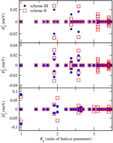
Figure 1: Components of the DMI vector $\vec{D}_{ij}$ for hcp Co. Results based on the present scheme (III) are compared with results calculated using scheme II Ebert and Mankovsky (2009). The calculations use a geometry with the direction of the DMI vector along the magnetization direction in the latter case, and the DMI direction perpendicular to the plane of the magnetization rotation in the former case.

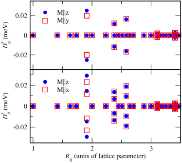
Figure 2: $D^{x}_{ij}$ (top) and $D^{y}_{ij}$ (bottom) components of the DMI vector for hcp Co calculated via scheme III for the different reference states: for $\theta=0$ and $\theta=\pi/2,\phi=0$ in the case of $D^{x}_{ij}$ (top) and for $\theta=0$ and $\theta=\pi/2,\phi=\pi/2$ in the case of $D^{y}_{ij}$ (bottom).

As another example we consider the DMI in the substitutional alloy Fe_1-xCo_xGe having the B20 crystal structure. Below the critical temperature $T_{c}$ and in the absence of an external magnetic field this material shows a helimagnetic structure. The helix wave vector changes with the Co concentration reaching a minimum at $x\approx 0.6$, where the helix chirality changes sign Grigoriev et al. (2014). On the basis of electronic structure calculations the $\vec{D}_{ij}$ interatomic interactions have been calculated using Eq. (18) up to $|\vec{R}_{i}-\vec{R}_{j}|=R_{max}=4a$ (with $a$ the lattice parameter). To treat the disorder on the (Fe,Co) sublattice, the calculations have been performed using the coherent potential approximation (CPA) alloy theory. Because of the non-trivial crystal structure and chemical disorder in the system, leading to a non-trivial analysis of the concentration dependent behavior of the DMI, it is more convenient to use a micromagnetic description for the DMI. The values for the corresponding parameters can be evaluated using the interatomic $\vec{D}_{ij}$ interactions by comparing the derivatives of the energy in the atomistic formulation, Eq. (9), and in the micromagnetic formulation, Eq. (22). This leads to the expression for the $y$-component of the micromagnetic DMI vector in terms of interatomic DMI vectors:

$$D^{yy} = \sum_{ij}D^{y}_{ij}\,(\vec{R}_{j}-\vec{R}_{i})_{y}\;.$$ (25)

Figure 3 represents the $D^{yy}$ element of the micromagnetic DMI vector as a function of the Co concentration in Fe_1-xCo_xGe. The values of the averaged interactions between the (Fe,Co) sites corresponding to different sublattices $m$, are shown in Fig. 3(a). As one can see, the various contributions $D^{yy}_{1-m}$ of the sublattices $m$ to the total component $D^{yy}=\sum_{m}D^{yy}_{1-m}$ show a rather different concentration dependence. In particular, they change sign at different Co concentration, while $D^{yy}$ changes sign at $x\approx 0.4$. As can be seen in Fig. 3(b), the $D^{yy}$ component of Co interaction with all surrounding (Fe,Co) sites changes sign at a lower concentration, slightly above $x=0.3$, while the corresponding value of $D^{yy}$ for Fe becomes positive at $x\approx 0.5$. The solid circles in Fig. 3(b) represent the results of calculations based on Eq. (24). As this value accounts for all interactions in the system, it slightly deviates from the $D^{yy}$ value that accounts only for interactions within (Fe,Co) sublattices, keeping however general trends concerning the concentration dependence. Despite certain differences, these results are in reasonable agreement with available experimental Grigoriev et al. (2014) and theoretical Kikuchi et al. (2016) data.

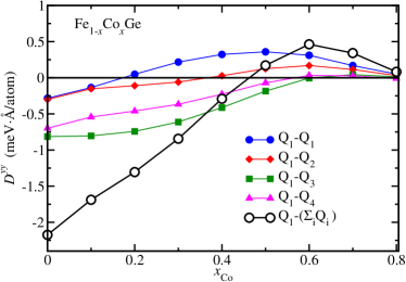
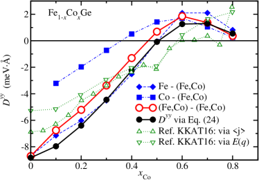
(a)  (b)

Figure 3: The $D^{yy}$ component of the micromagnetic DMI vector as a function of Co concentration in Fe_1-xCo_xGe, representing the average value of interactions of Mn and Fe magnetic moments (represented per atom) with the magnetic moments of 4 different (Fe,Co) sublattices (with $Q_{m}$ positions for (Fe,Co) atoms with $m=1-4$) (a); and the average interactions of the magnetic moment on the (Fe,Co) site with the magnetic moment on all surrounding (Fe,Co) neighbor sites, represented per unit cell. The results are compared with the results of calculations based on Eq. (24) (solid circles) as well as with theoretical results of Kikuchi et al. Kikuchi et al. (2016), shown by up- and down triangles, obtained in two different ways (for details see Ref. Kikuchi et al. (2016)) (b).

IV Appendix A

The expression for the DMI vector components derived within the present work differs slightly from those given previously Udvardi et al. (2003); Ebert and Mankovsky (2009). This is because there is some freedom concerning the scheme to map of the microscopic energy onto the extended Heisenberg Hamiltonian in Eq. (2). This point is illustrated in the following. Representing the components of the magnetic moments in spherical coordinates, the DMI-part of the Heisenberg Hamiltonian has the form

$${\cal H}_{\rm DM} = \sum_{ij}\vec{D}_{ij}\cdot(\hat{m}_{i}\times\hat{m}_{j})$$ (26)

$$= \sum_{ij}{D}^{x}_{ij}\,[\sin(\phi_{i})-\sin(\phi_{j})]\,\sin(\theta_{i})\,\cos(\theta_{j})$$

$$+\sum_{ij}{D}^{y}_{ij}\,[\cos(\phi_{j})-\cos(\phi_{i})]\,\sin(\theta_{i})\,\cos(\theta_{j})$$

$$+\sum_{ij}{D}^{z}_{ij}\,[\cos(\phi_{i})\,\sin(\phi_{j})-\cos(\phi_{j})\,\sin(\phi_{i})]\,$$

$$\times\sin(\theta_{i})\,\sin(\theta_{j})\;.$$

To simplify the discussion, let’s consider a system with one sublattice and focus on the last term with the magnetization direction $\vec{m}||\hat{z}$ (i.e. $\theta=0$ for all local magnetic moments in the reference state). In this case the $D^{z}_{ij}$ component of the DMI vector can be represented by the second derivative of the energy with respect to the angle $\theta_{i(j)}$:

$$D^{z}_{ij}=\frac{1}{2}\left[\frac{\partial^{2}E}{\partial\theta_{i}\partial\theta_{j}}\bigg{|}_{\begin{subarray}{c}\phi_{i}=0\\ \phi_{j}=\pi/2\\ \theta_{i(j)}=0\end{subarray}}-\frac{\partial^{2}E}{\partial\theta_{i}\partial\theta_{j}}\bigg{|}_{\begin{subarray}{c}\phi_{j}=0\\ \phi_{i}=\pi/2\\ \theta_{i(j)}=0\end{subarray}}\right]\;.$$ (27)

This means that the $D^{z}_{ij}$ component of the DMI vector is evaluated as the energy difference between the reference state ($\hat{m}_{i}||\hat{z}$ for all $i$) and the state with two magnetic moments having small components in the $x-y$ plane, which are orthogonal to each other, giving a maximal energy change due to the DM interaction between these in-plane components.

Similar to Eq.  (11) an evaluation can also be done considering the energy change due to tilting of two magnetic moments. In this case one has:

$$K_{ij}^{(1)}(\vec{r}) = -\frac{1}{\pi}\mbox{Im}\,\mbox{Tr}\int^{\mu}dE\,[({\cal H}-\mu)\,G(\vec{r},\vec{r}\,^{\prime},E)-({\cal H}_{0}-\mu)\;G_{0}(\vec{r},\vec{r}\,^{\prime},E)]$$ (28)

$$= -\frac{1}{\pi}\mbox{Im}\,\mbox{Tr}\int^{\mu}dE\,(H_{0}-\mu)\;\Delta G(\vec{r},\vec{r}\,^{\prime},E)-\frac{1}{\pi}\mbox{Im}\,\mbox{Tr}\int^{\mu}dE\,(\delta V_{i}+\delta V_{j})\,G_{0}(\vec{r},\vec{r}\,^{\prime},E)$$

$$-\frac{1}{\pi}\mbox{Im}\,\mbox{Tr}\int^{\mu}dE\,\int_{\Omega}d^{3}r^{\prime\prime}\,(\delta V_{i}(\vec{r})+\delta V_{j}(\vec{r}))\,G_{0}(\vec{r},\vec{r}\,^{\prime\prime},E)\,(\delta V_{i}(\vec{r}\,^{\prime\prime})+\delta V_{j}(\vec{r}\,^{\prime\prime}))\,G_{0}(\vec{r}\,^{\prime\prime},\vec{r}\,^{\prime},E)\;,$$

with $\delta V_{i}=\beta\vec{\sigma}\cdot(\hat{m}_{i}-\hat{z})B_{xc}^{i}(\vec{r})$. Eq.  (28) can be used for the evaluation of the elements of the exchange coupling tensor by calculating the second energy derivative $\frac{\partial^{2}K^{(1)}}{\partial\alpha_{1}\partial\beta_{2}}$ with $K^{(1)}=\int_{\Omega}K^{(1)}(r)d^{3}r$. The first two terms yield 0, while the third term gives the elements of the exchange coupling tensor similar to the one used in Ebert and Mankovsky (2009). For the particular case this leads to the $z$ component of the DMI vector given by Eq.  (27), as provided by scheme II Ebert and Mankovsky (2009).

To discuss an alternative possibility, let’s represent the last term of Eq.  (IV) as follows

$$\sum_{ij}{D}^{z}_{ij}\,\sin(\phi_{j}-\phi_{i})\,\sin(\theta_{i})\,\sin(\theta_{j})\;.$$

In this case, taking the direction of magnetization within the plane, implying $\theta=\pi/2$, $D^{z}_{ij}$ gives the energy variation due to tilting of two magnetic moments away from a collinear orientation by the small angles $\phi_{j}$ and $\phi_{i}$. In this case $D^{z}_{ij}$ can be represented through the first derivatives of the energy with respect to $\phi_{j}$ and $\phi_{i}$

$$D^{z}_{ij} = \frac{1}{2}\left[\frac{\partial E}{\partial\phi_{j}}\bigg{|}_{\begin{subarray}{c}\theta_{i},\theta_{j}=\pi/2\\ \phi_{i},\phi_{j}=0\\ \hat{n}=\hat{z}\end{subarray}}-\frac{\partial E}{\partial\phi_{i}}\bigg{|}_{\begin{subarray}{c}\theta_{i},\theta_{j}=\pi/2\\ \phi_{i},\phi_{j}=0\\ \hat{n}=\hat{z}\end{subarray}}\right]$$ (29)

$$= -\frac{1}{2}\left[R_{ji}^{xy}\bigg{|}_{\begin{subarray}{c}\theta_{i(j)}=\pi/2\\ \phi_{i},\phi_{j}=0\end{subarray}}-R_{ji}^{yx}\bigg{|}_{\begin{subarray}{c}\theta_{i(j)}=\pi/2\\ \phi_{i},\phi_{j}=0\end{subarray}}\right]\;,$$

where $\hat{n}$ is the direction of the torque $\vec{R}^{ij}_{j}$, and $R^{z,ij}_{i}$ is the projection of the torque acting on magnetic moment $\vec{m}_{i}$, originated due to the DMI and given by the expression

$$R_{ji}^{xy} = \frac{1}{\pi}\mbox{Im}\,\mbox{Tr}\int^{\mu}dE\,$$ (30)

$$\times\underline{T}^{j,x}(E)\,\underline{\tau}^{ji}(E)\,\underline{T}^{i,y}(E)\,\underline{\tau}^{ij}(E)\Big{]}\;.$$

Here it is assumed that the magnetic moment is oriented along the $x$ direction, and $\underline{T}^{i,\alpha}(E)$ represents the matrix elements of the operator ${\cal T}^{i,\alpha}=\beta\sigma_{\alpha}B_{xc}^{i}(\vec{r})$.

This alternative formulation is similar to the one worked out for the definition of the DMI by Katsnelson et al. Katsnelson et al. (2010) and is in line with the derivation represented above in this work Eq. (18).

V Acknowledgement

Financial support by the DFG via SFB 689 (Spinphänomene in reduzierten Dimensionen) is gratefully acknowledged.

References

- Bogdanov and Hubert (1994) A. Bogdanov and A. Hubert, J. Magn. Magn. Materials 138, 255 (1994), ISSN 0304-8853, URL http://www.sciencedirect.com/science/article/pii/0304885394900469.
- Roszler et al. (2006) U. K. Roszler, A. N. Bogdanov, and C. Pfleiderer, Nature 442, 797 (2006), ISSN 0028-0836, URL http://dx.doi.org/10.1038/nature05056.
- Schulz et al. (2012) T. Schulz, R. Ritz, A. Bauer, M. Halder, M. Wagner, C. Franz, C. Pfleiderer, K. Everschor, M. Garst, and A. Rosch, Nature Physics 8, 301 (2012), URL http://dx.doi.org/10.1038/nphys2231.
- Neubauer et al. (2009) A. Neubauer, C. Pfleiderer, B. Binz, A. Rosch, R. Ritz, P. G. Niklowitz, and P. Böni, Phys. Rev. Lett. 102, 186602 (2009), URL http://link.aps.org/doi/10.1103/PhysRevLett.102.186602.
- Togawa et al. (2012) Y. Togawa, T. Koyama, K. Takayanagi, S. Mori, Y. Kousaka, J. Akimitsu, S. Nishihara, K. Inoue, A. S. Ovchinnikov, and J. Kishine, Phys. Rev. Lett. 108, 107202 (2012), URL http://link.aps.org/doi/10.1103/PhysRevLett.108.107202.
- Togawa et al. (2013) Y. Togawa, Y. Kousaka, S. Nishihara, K. Inoue, J. Akimitsu, A. S. Ovchinnikov, and J. Kishine, Phys. Rev. Lett. 111, 197204 (2013), URL http://link.aps.org/doi/10.1103/PhysRevLett.111.197204.
- Udvardi et al. (2003) L. Udvardi, L. Szunyogh, K. Palotás, and P. Weinberger, Phys. Rev. B 68, 104436 (2003), URL http://link.aps.org/doi/10.1103/PhysRevB.68.104436.
- Ebert and Mankovsky (2009) H. Ebert and S. Mankovsky, Phys. Rev. B 79, 045209 (2009), URL http://link.aps.org/doi/10.1103/PhysRevB.79.045209.
- Liechtenstein et al. (1987) A. I. Liechtenstein, M. I. Katsnelson, V. P. Antropov, and V. A. Gubanov, J. Magn. Magn. Materials 67, 65 (1987), URL http://www.sciencedirect.com/science/article/pii/0304885387907219.
- Heide et al. (2008) M. Heide, G. Bihlmayer, and S. Blügel, Phys. Rev. B 78, 140403 (2008), URL http://link.aps.org/doi/10.1103/PhysRevB.78.140403.
- Heide et al. (2009) M. Heide, G. Bihlmayer, and S. Blügel, Physica B: Condensed Matter 404, 2678 (2009), ISSN 0921-4526, proceedings of the Workshop: At the Frontiers of Condensed Matter IV. Current Trends and Novel Materials, URL http://www.sciencedirect.com/science/article/pii/S0921452609004177.
- Freimuth et al. (2014) F. Freimuth, S. Blügel, and Y. Mokrousov, J. Phys.: Cond. Mat. 26, 104202 (2014), eprint 1308.5983, URL http://stacks.iop.org/0953-8984/26/i=10/a=104202.
- Koretsune et al. (2015) T. Koretsune, N. Nagaosa, and R. Arita, Scientific Reports 5, 13302 (2015), URL http://dx.doi.org/10.1038/srep13302.
- Engel and Dreizler (2011) E. Engel and R. M. Dreizler, Density Functional Theory – An advanced course (Springer, Berlin, 2011), URL http://www.springerlink.com/content/m246q2.
- Rose (1961) M. E. Rose, Relativistic Electron Theory (Wiley, New York, 1961), URL http://openlibrary.org/works/OL3517103W/Relativistic_electron_theory.
- H. Ebert et al. (2012) H. Ebert et al., The Munich SPR-KKR package, version 6.3, http://olymp.cup.uni-muenchen.de/ak/ebert/SPRKKR (2012), URL http://olymp.cup.uni-muenchen.de/ak/ebert/SPRKKR.
- Ebert et al. (2011) H. Ebert, D. Ködderitzsch, and J. Minár, Rep. Prog. Phys. 74, 096501 (2011), URL http://stacks.iop.org/0034-4885/74/i=9/a=096501.
- Ebert et al. (2016) H. Ebert, J. Braun, D. Ködderitzsch, and S. Mankovsky, Phys. Rev. B 93, 075145 (2016), URL http://link.aps.org/doi/10.1103/PhysRevB.93.075145.
- Grigoriev et al. (2014) S. V. Grigoriev, S.-A. Siegfried, E. V. Altynbayev, N. M. Potapova, V. Dyadkin, E. V. Moskvin, D. Menzel, A. Heinemann, S. N. Axenov, L. N. Fomicheva, et al., Phys. Rev. B 90, 174414 (2014), URL https://link.aps.org/doi/10.1103/PhysRevB.90.174414.
- Kikuchi et al. (2016) T. Kikuchi, T. Koretsune, R. Arita, and G. Tatara, Phys. Rev. Lett. 116, 247201 (2016), URL https://link.aps.org/doi/10.1103/PhysRevLett.116.247201.
- Katsnelson et al. (2010) M. I. Katsnelson, Y. O. Kvashnin, V. V. Mazurenko, and A. I. Lichtenstein, Phys. Rev. B 82, 100403 (2010), URL https://link.aps.org/doi/10.1103/PhysRevB.82.100403.