Lyth Bound, eternal inflation and future cosmological missions

Abstract

In this paper we provide a new expression for the variation of the inflaton field $\Delta\phi$ during the horizon crossing epoch in the context of single field slow roll inflationary models. Such an expression represents a generalization of the well-know Lyth bound. We also explore the consequences of a detection of permille order of the tensor-to-scalar ratio amplitude, $r$, as well as an improvement on the estimation of the scalar spectral index, $n_{s}$ and its running $\alpha_{s}$, by the upcoming cosmic macrowave background (CMB) polarization experiments that will provide plausible constraints on the quantity $\Delta\phi$ during the horizon exit moment. In addition we discuss the relation between the local variation of the field and the possibilities of an eternal inflation. The results of the analysis are completely model independent.

I Introduction

The inflationary stage is the widely accepted mechanism to explain the physics of the early universe 1 . The simplest and most promising version involves a single field slow-roll inflation where an ordinary scalar field $\phi$ (neutral, homogeneous, minimally coupled to gravity and canonically normalized) explores an appropriate effective potential $V(\phi)$ to realize a quasi de-Sitter evolution of the spacetime, if the slow roll condition $\dot{\phi}^{2}\ll V(\phi)$ holds long enough. This scalar field is often called inflaton field and the function $V(\phi)$ is the inflationary potential. Although inflation explains several features of our universe (absence of monopoles, flatness, homogeneity and isotropy, adiabatic and scale invariant fluctuations) we need to address and resolve compelling open issues. One of these is the nature of the scalar field $\phi$ and the size of the distance covered by $\phi$ during inflation, $\Delta\phi$. Several authors used to say that a trans or super-planckian excursion of the inflaton field, $\Delta\phi>M_{p}$ could be very problematic especially from the standpoint of the low energy effective field theory (EFT) with a given Planck cut-off 2 ; 3 ; 4 . However, in the last years it has been shown that the question is not general: the well-known $\alpha$-attractor models of inflation do not suffer from this problem. In any case, Lyth derived a bound (see 2 ) for the value assumed by $\Delta\phi$ in terms of the amplitude $r$ of the primordial gravitational waves produced during inflation (in the context of slow-roll inflationary models). This quantity is known as Lyth Bound and represents an estimation of $\Delta\phi$ at horizon crossing: $\Delta\phi_{H.c.}$. In the last years, different studies concerning the variation of the field and the Lyth bound itself have been done 5 ; 6 ; 7 . In future, foreseen CMB polarization missions (8 ; 9 ; 10 ; 11 ; 12 ) and gravitational waves experiments (13 ) will constrain cosmological observables better than the current available data, 14 ; 15 . In particular, they will be able to explore values of $r$ of the order of $10^{-3}$ and to reduce the uncertainty on $n_{s}$ and $\alpha_{s}$ better than a factor 3. Therefore, in this paper we provide a new slow-roll expansion of the standard Lyth bound to take into account our (current and foreseen) knowledge about the scalar spectral index, $n_{s}$, and the running of the scalar spectral index, $\alpha_{s}$. Then, we present plausible constraints on $\Delta\phi$ at horizon crossing with respect to future cosmological results. The estimation of the running of the scalar perturbations, $\alpha_{s}$, could be important to evaluate the possibility of an eternal inflation (see 16 ; 17 ; 18 ; 19 ), as outlined by W.Kinney and K.Freese in 20 . Therefore, we will discuss the implication of an eternal inflation on the local variation of the field. The paper is organized in the following way. In Sec. II we summarize the problem of the variation of the field and we introduce the standard definition of Lyth Bound and finally, we use the inflationary flow equations to generalize the Lyth formula. In Sec. III we discuss what we can expect on $\Delta\phi_{H.c.}$ in view of future polarization missions and we explore the relation between eternal inflation and $\Delta\phi_{H.c.}$. Finally, Sec. IV is dedicated to our findings. In this manuscript we use the particle natural units, $c=\hbar=1$, $m_{p}$ indicates the Planck mass and $M_{p}$ is the reduced Planck mass, with $M^{2}_{p}=m_{p}^{2}/8\pi$.

II Slow roll inflation and the variation of the scalar field

II.1 Effective field theory, super-planckian excursions and Lyth Bound

The dynamics of a slow roll inflationary universe can be described within a Hamilton-Jacobi picture by the following system of coupled equations:

$$V(\phi)=3M^{2}_{p}H^{2}(\phi)-2M^{2}_{p}H^{\prime}(\phi),$$ (1)

$$\dot{\phi}=-2M^{2}_{p}H^{\prime}(\phi)$$ (2)

where we can assume $\dot{\phi}<0$ and $H^{\prime}(\phi)>0$. As remarked in Sec. I, we have a quasiexponential evolution of the spacetime. At the same time, the scalar field gets a slow evolution (over the first stage of inflation) because $\dot{\phi}^{2}\ll V(\phi)$. At first order, the resulting dynamics is well described by the first two Hubble slow roll parameters:

$$\epsilon(\phi)=2M^{2}_{p}\left(\frac{H^{\prime}(\phi)}{H(\phi)}\right)^{2},\quad\eta(\phi)=2M^{2}_{p}\left(\frac{H^{\prime\prime}(\phi)}{H(\phi)}\right)$$ (3)

where $\sqrt{\epsilon}>0$ if $\dot{\phi}<0$. The nature of the scalar field $\phi$ is an open issue: it could be a fundamental particle field (for instance, an Higgs field 20 ) or an auxiliary field emerging from a modification of gravity (for example, Starobinisky $R^{2}$ model or its extensions 21 ; 22 ). In any case it is common believed that the inflaton could be an effective light scalar degree of freedom in a low energy-limit description of some more fundamental quantum gravity cosmological theory. This piece of evidence led people to make the following observations. We can think inflation as emerging from a low energy effective field theory (EFT) with some Planck cut-off $\Lambda$. Therefore, the corresponding effective (slow roll) inflationary lagrangian is obtained integrating out the Planck-scale (quantum gravity) degrees of freedom (see 23 for a review). As a result, the slow roll effective potential $V(\phi)$ receives an infinite number of corrections, given by Planck suppressed operators $\mathcal{O}^{(n)}$ 2 ; 3 ; 4

$$\mathcal{L(\phi,\partial_{\mu}\phi}) = -\frac{1}{2}\partial_{\mu}\phi\partial^{\mu}\phi-V(\phi)\left[1+\sum_{n=1}^{\infty}\frac{\mathcal{O}^{(n)}}{M_{p}^{n-4}}\right]$$

$$= -\frac{1}{2}\partial_{\mu}\phi\partial^{\mu}\phi-V(\phi)\left[1+\sum_{n=1}^{\infty}\lambda_{n}\left(\frac{\phi}{M_{p}}\right)^{n}\right].$$

In particualar, the operators $\mathcal{O}^{(n)}$ result in power of $\phi$. The $\lambda_{n}$ are the Wilson coefficients, typically of order $1$. This means we have an infinite number of corrections of the same order. Now, as stressed by different authors (see 2 ; 3 ), if the scalar field assumes subplanckian values, $\phi\ll M_{p}$, i.e is small, the series is asymptotically convergent. This suggest we can describe inflation by an EFT whether $\Delta\phi\ll M_{p}$ over the entire inflationary history. On the other side, if the field takes on trans or super-Planckian values, $\phi>M_{p}$, the series is divergent. Then, under this condition, an EFT-description of inflation it is hard to realize because higher-order operator terms become important and the balance between the shape and the height of the potential is not guaranteed (see again 2 ; 3 ). For example, operator terms of the form:

$$\Delta V_{2}(\phi)\sim V(\phi)\frac{\phi^{2}}{M_{p}^{2}}$$ (5)

contributes to the slow roll parameter $\eta$ with order $1$ not providing a sufficient amount of inflation (this is the so called $\eta$-problem, 23 ). At this point, as summarized in 23 , we can make a sense to the EFT slow roll models only if the Wilson coefficients are small, $\lambda_{n}\ll 1$. This is a distinct possibility if we introduce a symmetry for the effective lagrangian with the prescription that such a symmetry is also recognized in the UV completion of our EFT (e.g. in superstring theory, 24 ; 25 ) to ensure that it is also realized even at the fundamental Planck-scale 26 . A typical example is the shift symmetry. Indeed shift symmetry is not broken by perturbative corrections of quantum gravity. In principle, it could be broken by nonperturbative effects although they are so small to result negligible 27 . Actually, other authors like Linde (see 28 for a review), state that the problem of $\Delta\phi$-size and therefore the values assumed by the scalar field is a relative question. In fact, one should just make sure that the energy density is sub-Planckian, $V(\phi)<M^{4}_{p}$ in order to avoid quantum gravity effects (while the field can still assumes larger values in Planck units). However, the current state of the art is a little bit different. For instance, in the last years A.Linde, R.Kallosh and others developed a new important class of inflationary models called $\alpha$-attractors models which the most advanced version is realized in the supergravity framework 29 . These models are characterized by an asymptotic flatness region for large value of $\phi$ and they interpolate a broad range of predictions in the $(n_{s},r)$-plane. Furthermore, they do not suffer from the problem discussed before because the asymptotic flatness of the inflationary potential is preserved by dangerous quantum corrections as shown in 30 . However, the excursion of the scalar field $\Delta\phi$ over the inflationary phase shows a lower limit thanks to Lyth 2 . This limit can be derived using different approach. One way is to consider the Eq.(2) and rewrite the derivative with respect to time in a derivative with respect to the number of $e$-foldings $N$. As a result, we get:

$$\frac{d\phi}{dN}=\sqrt{2}M_{p}\sqrt{\epsilon(\phi)}.$$ (6)

This equation is particularly important because allows to reword a $\phi$-type derivative in a $N$-type derivative. Note that this quantity is modulated by the first slow roll parameter $\epsilon$. The slow roll condition for the inflaton dynamics implies $r\sim 16\epsilon$ and both of these parameters are slowly varying. Then, the variation of the field along the horizon crossing period can be written as:

$$\frac{\Delta\phi_{h.c.}}{M_{p}}=\sqrt{\frac{r}{8}}|\Delta N|\quad\mbox{ or}\quad\frac{\Delta\phi_{h.c}}{m_{p}}=\sqrt{\frac{r}{64\pi}}|\Delta N|.$$ (7)

Nevertheless, the observable scales from which we deduce the value of or the bounds for the inflationary parameters like $n_{s},r,\alpha_{s},...$, correspond to multipoles $2<l<100$. These scales leave the Hubble horizon $R_{H}=1/H$ along a period of $\Delta N\sim 4$ $e$-foldings. Therefore, we can state that the total excursion of the scalar field is larger than:

$$\frac{\Delta\phi}{m_{p}}\geq\sqrt{\frac{r}{4\pi}}.$$ (8)

This result is model dependent in the sense that, each model of inflation is characterized by a minimal excursion modulated by the amplitude $r$. Let us assume that the number of $e$-foldings between the horizon crossing epoch and the end of inflation epoch is $N_{*}\sim 60$. Then, for a quadratic potential $V(\phi)\sim m^{2}\phi^{2}$ we have:

$$\frac{\Delta\phi_{h.c.}}{m_{p}}\sim 0.1$$ (9)

while for a quartic potential $V(\phi)\sim\lambda\phi^{4}$ the corresponding variation is

$$\frac{\Delta\phi_{h.c.}}{m_{p}}\sim 0.14.$$ (10)

Note that, we have to keep in mind that different potentials can produce the same $r$ and so the same $\Delta\phi$. On the other hand, a precise detection of the tensor-to-scalar ratio plays an important role to determine the minimal displacement of the field beyond the specific model. However, the Lyth Bound is a first order result. In the future, different cosmological missions aim to improve the current knowledge about the inflationary parameters. In this respect, we want to generalize the Lyth Bound in order to include the $n_{s}$ and $\alpha_{s}$ contributions and exploring so possible constraints on $\Delta\phi_{H.c.}$ at next orders.

II.2 Generalizing Lyth Bound

In this section we aim to derive a higher order expression of the Lyth Bound. To reach this goal, the slow roll parameters and the related inflationary flow equations are the fundamental tools. The Hubble slow roll parameters are defined by the following hierarchy of variables 31 :

$$\epsilon(\phi) = 2M^{2}_{p}\left(\frac{H^{\prime}}{H}\right)^{2}$$ (11)

$$\beta^{(n)}(\phi) = (2M^{2}_{p})^{n}\left[\frac{H^{\prime n-1}H^{(n+1)}}{H^{n}}\right]$$ (12)

where $\eta=\beta^{(1)}$, $\xi^{2}=\beta^{(2)}$, $\sigma^{3}=\beta^{(3)}$ … with $\sqrt{\epsilon}>0$ for $\dot{\phi}<0$, as remarked in Sec. II. The slow roll parameters are not constant in general but they change as the scalar field evolves. However, as explained by Easther, Kinney and Powell in 3 , the evolution of the slow roll parameters could be very slow (for example during the horizon crossing epoch) in some phases of inflation compared to other moments (the last $e$-folds of inflationary expansion). Mathematically, the evolution of the $\beta_{i}(\phi)$ are well-described by the system of inflationary flow equations, in which, for sake of convenience, the slow roll parameters are suitably expressed as functions of the number of $e$-foldings. In particular, we can write

$$\frac{d\epsilon}{dN} = 2\epsilon(\eta-\epsilon)$$ (13)

$$\frac{d\eta}{dN} = \xi^{2}-\epsilon\eta$$ (14)

$$\frac{d\beta^{(n)}}{dN} = \left[(n-1)\eta-n\epsilon\right]\beta^{(n)}+\beta^{(n+1)}.$$ (15)

Greater details can be found in references 32 ; 33 . At this point, we can follow the method used in 3 and write down a Taylor expansion of the scalar field (as a function of the number of $e$-foldings) around the horizon crossing of the observable scales

$$\phi(N)=\phi(N_{*})+\phi^{\prime}(N_{*})\Delta N+\frac{1}{2!}\phi^{\prime\prime}(N_{*})\Delta N^{2}+...$$ (16)

where ^′ indicates a derivative with respect to $N$ and $\Delta N=N-N_{*}$ Assuming again that $\phi$ is decreasing along the inflationary evolution and that $N_{*}>N$, we can rewrite the Taylor expansion as follows:

$$\Delta\phi=+\phi^{\prime}(N_{*})|\Delta N|-\frac{1}{2!}\phi^{\prime\prime}(N_{*})|\Delta N|^{2}+...$$ (17)

where $\Delta\phi=\phi_{*}-\phi$ and $|\Delta N|=-(\Delta N)$. Generalizing, we have

$$\Delta\phi=\sum_{n=1}^{\infty}c_{n}|\Delta N|^{n},\quad c_{n}=(-1)^{n+1}\phi^{(n)}(N_{*}).$$ (18)

The first order derivative of the expansion is the previous basic equation, Eq.(19)

$$\frac{d\phi}{dN}=\sqrt{2}M_{p}\sqrt{\epsilon(\phi)}.$$ (19)

Using the flow equations we can derive the higher order derivatives of the field in terms of the slow roll parameters. For example, next orders result in

$$\frac{d^{2}\phi}{dN^{2}}=\sqrt{2}M_{p}\sqrt{\epsilon}\left(\eta-\epsilon\right),$$ (20)

$$\frac{d\phi^{3}}{dN^{3}}=\sqrt{2}M_{p}\sqrt{\epsilon}\left(3\epsilon^{2}+\eta^{2}-5\epsilon\eta+\xi^{2}\right)$$ (21)

and

$$\frac{d\phi^{4}}{dN^{4}}=\sqrt{2}M_{p}\sqrt{\epsilon}\left[f_{1}(\epsilon,\eta,\xi^{2})+f_{2}(\epsilon,\eta,\xi^{2},\sigma^{3})\right]$$ (22)

where

$$f_{1}(\epsilon,\eta,\xi^{2})=(\eta-\epsilon)(15\epsilon^{2}+\eta^{2}-15\epsilon\eta+\xi^{2}),$$ (23)

$$f_{2}(\epsilon,\eta,\xi^{2},\sigma^{3})=(\xi^{2}-\epsilon\eta)(2\eta-5\epsilon)$$

$$+\xi^{2}(\eta-2\epsilon)+\sigma^{3}$$ . (24)

Here $\sigma^{3}$ is the fourth slow roll parameter. At this point, we can calculate the derivatives at horizon crossing moment $t_{*}$ (or $N_{*}$, let us say). In doing so, we have to reword the slow roll parameters in terms of the inflationary observables. At first order, we have

$$\epsilon\sim\frac{r}{16},\quad\eta\sim\frac{1}{2}(n_{s}-1)+\frac{r}{8}$$ (25)

and

$$\xi^{2}\sim 5\epsilon\eta-4\epsilon^{2}-\frac{1}{2}\alpha_{s}.$$ (26)

Substituting these information in the expansion Eq.(18) with $|\Delta N|\sim 4$ $e$-folds, we have (at the third order, for instance)

$$\frac{\Delta\phi_{h.c}}{m_{p}}\sim\sqrt{\frac{r}{4\pi}}\Big{\{}\Pi_{0}-\Pi_{1}-\Pi_{2}+...\Big{\}}$$ (27)

where:

$$\Pi_{0} = 1$$ (28)

$$\Pi_{1} = (n_{s}-1)+\frac{r}{8}$$ (29)

$$\Pi_{2} = \frac{8}{3}\left(\frac{r}{16}\right)^{2}-\frac{8}{3}\left[\frac{1}{2}(n_{s}-1)+\frac{r}{8}\right]^{2}+\frac{4}{3}\alpha_{s}$$ (30)

where $\Pi_{1}=\Pi_{1}(r,n_{s})$, $\Pi_{2}=\Pi_{2}(r,n_{s},\alpha_{s})$. The first term of the expansion is the standard Lyth Bound. The second order term, linear in $n_{s}$, is the result found by R.Easther et all in 3 . Finally, the last term is the new corrections that take into account the contribution of the running of the scalar spectral index and the quadratic order in $r$ and $n_{s}$. Note that, the contribution of $\alpha_{s}$ in our formula appears with a negative sign

$$\frac{\Delta\phi_{h.c}}{m_{p}}\sim-\frac{4}{3}\alpha_{s}$$ (31)

Therefore a negative value for $\alpha_{s}$ pushes the local variation $\Delta\phi$ to larger values. On the contrary, if $\alpha_{s}$ results to be positive, the excursion receives a negative contribution. In the next section, we use our third order result to explore the constraints we may have on the variation $\Delta\phi_{h.c}$ in terms of the expected results of next generation experiments and we discuss the implication of an eternal inflation on the variation of the field.

III What we can expect by upcoming cosmological missions?

III.1 Monte Carlo simulation

The current state-of-the art for the values of the main inflationary parameters is the following (for detailed papers see 11 ; 12 :

$$n_{s}=0.9680\pm 0.006,\quad r<0.07\mbox{ at 95\% C.L.}$$ (32)

and

$$\alpha_{s}=\frac{dn_{s}}{d\ln k}=-0.0033\pm 0.0074$$ (33)

However, the above limits could rapidly improve in the close future due to the next generation of cosmological experiments, like polarization missions of the cosmic macrowave background (CMB) or gravitational waves (GW) detection missions. These new missions aim to improve the knowledge on $n_{s}$ and $\alpha_{s}$ and to probe scales of the order of $10^{-3}$ for the tensor-to-scalar ratio amplitude, $r$ (or better in the best scenario, 8 ; 9 ; 10 ; 11 ; 12 ; 13 ). In this regard, we investigate the variation of the field over the first $4$ $e$-folds (more or less) of inflationary expansion. To do this, we consider a multivariate Gaussian $\mathcal{G}(r,n_{s},\alpha_{s})$ distribution for the parameters $(r,n_{s},\alpha_{s})$ with

1. $\mu_{r}=0.003,0.004,0.005$

2. $\mu_{n_{s}}=0.9620,0.9650,0.9680$

3. $\mu_{\alpha_{s}}=-0.0005,-0.0015,-0.0025$

with uncertainties $\sigma_{r}=0.0001$, $\sigma_{n_{s}}=0.002$, $\sigma_{\alpha_{s}}=0.0023$, respectively. Furthermore, we set to zero (for simplicity) all the correlation coefficients: $\rho_{rn_{s}}=\rho_{r\alpha_{s}}=\rho_{n_{s}\alpha_{s}}=0$. In Table I, we report the simulation results for the size of $\Delta\phi_{h.c}$ for the three different assumed values of the tensor-to-scalar ratio. In this case, we report the results for all of the three expressions $\Delta\phi_{h.c}(\Pi_{i})$. On the other side, in Table II and in Table III we skip the term $\Delta\phi_{h.c}(\Pi_{0})$ and $\Delta\phi_{h.c}(\Pi_{1})$, respectively. This is due to the structure of the expressions. Furthermore, Fig.(1) and in Fig.(2) show the resulting distribution functions for the minimum value of $\Delta\phi$ supposing a detection of primordial tensor modes given by a forthcoming CMB baloon polarization mission or GW mission while Fig.(3) and Fig.(4) report the associated dispersion relations $\Delta\phi_{h.c}(\Pi_{1})/\Delta\phi_{h.c}(\Pi_{0})$ and $\Delta\phi_{h.c}(\Pi_{2})/\Delta\phi_{h.c}(\Pi_{0})$, respectively. In both cases, we assume the current data for the sampling of $n_{s}$ and $\alpha_{s}$. Now, these Monte-Carlo simulations show a couple of properties. First of all, we can deduce from Table I the inclusion of the scalar spectral index $n_{s}$ and the running $\alpha_{s}$ produces a larger $\Delta\phi_{h.c}$. Second, the $1$-$\sigma_{\Delta\phi_{h.c}}$-value turns out to be larger as the slow roll reconstruction become deeper. Somehow, this is an expected result and it is originated by the introduction of more uncertainty due to the new parameters. On the other hand, Table II tells us that the variation of the field become smaller as $n_{s}$ increases. In fact, the scalar spectral index, always appears in the $\Delta\phi_{h.c}$ expression like $1-n_{s}$. Therefore, when $n_{s}$ gets larger values, the previous term approaches to zero so it is a subdominant contribution. The last table (Table III) shows that a bigger running index (in modulus) implies a larger excursion because of Eq.(31).

III.2 Lyth Bound and eternal inflation

The inflationary mechanism could lead to a very interesting and spectacular consequence: an infinitely self-reproducing state commonly called eternal inflation. The eternal inflation process was firstly outlined by A.Linde, P.Steinhardt and A.Vilenkin (see 16 ; 17 ) in the framework of new inflation. Afterwards, A.Linde realized that such a mechanism could be also possible in the chaotic inflationary scenario 18 (see also, 19 for greater details). In this second case, the eternal inflation stage is laid down when the inflaton field explores a region $\Sigma$ of the inflationary potential in which quantum fluctuations of the field $\delta\phi$ are larger then the classical variation ones, $\Delta\phi$. This leads to a very interesting implications about the amplitude of the metric perturbations as pointed out by A.Linde in the second of references 19 and summarized in 34 ; 35 : the power spectrum of the scalar metric perturbations must exceed the unity on those physical scales related to $\Sigma$

$$P_{s}(k)=A_{s}\left(\frac{k}{k_{*}}\right)^{f(k,k_{*})}>1\mbox{ for all }k\in\mathcal{I}_{\Sigma}(k)$$ (34)

where $\mathcal{I}_{\Sigma}(k)$ is the set of scales $k$ related to the portion $\Sigma$ of inflationary potential, $k_{*}$ is the pivot scale for probing the cosmological parameters and the function $f(k,k_{*})$ is given by

$$f(k,k_{*})=(n_{s}-1)+\alpha_{s}\ln\left(\frac{k}{k_{*}}\right)+\beta_{s}\ln^{2}\left(\frac{k}{k_{*}}\right)+...$$ (35)

in which $\beta_{s}$ and the higher order terms represent the running-of-the-running, the running-of-the-running-of-the-running and so on. Who is $I_{\Sigma}(k)$? We should note that the current cosmological results show a very low $A_{s}$ ($A_{s}\simeq 2.2\times 10^{-9}$, see 14 ; 15 ) therefore we can be fairly confident the observable and accessible region of $V(\phi)$ does not provide an eternal inflationary epoch. Then, we can expect an increase (at least) of the order of $10^{9}$ on $P_{s}(k)$ only at extremely large scales $k\ll k_{*}$, beyond our horizon in principle. How can we get $P_{s}(k)\geq 1$? In general, we can get such a condition by proper choices of the function Eq.(35), i.e., by proper choice of the cosmological parameters. Then, if we truncate the series at higher orders, the condition Eq.(34) is provided by a large number of choices, generally. However, we may imagine that the power spectrum is modulated only by the scalar spectral index and by a non null and constant $\alpha_{s}$:

$$\alpha_{s}\neq 0,\quad\mbox{ and }\quad\frac{d\alpha_{s}(k)}{d\ln k}=0$$ (36)

From this point of view, one can use the running as the only degree of freedom or “temperature parameter” to study the transition to a blue spectrum $P(k)>1$. We can call the threshold value of the running preventing the eternal inflation, $\alpha^{*}_{s}$ and find 35 :

$$\alpha^{*}_{s}=\frac{(1-n_{s})^{2}}{4\ln A_{s}}$$ (37)

Therefore, we may argue that:

$$\alpha_{s} < \alpha^{*}_{s}\mbox{ eternal inflation does not occur }$$ (38)

$$\alpha_{s} > \alpha^{*}_{s}\mbox{ eternal inflation occurs }$$ (39)

For instance,

$$n_{s}\sim 0.9620,\quad\alpha^{*}_{s}\sim-1.8109\times 10^{-5}$$ (40)

$$n_{s}\sim 0.9650,\quad\alpha^{*}_{s}\sim-1.5363\times 10^{-5}$$ (41)

$$n_{s}\sim 0.9680,\quad\alpha^{*}_{s}\sim-1.2842\times 10^{-5}$$ (42)

In the previous section we derived an expression of the Lyth Bound in terms of $\alpha_{s}$. Then, we can distinguish which are the minimum variations of the field related to an eternal inflation (EI) stage with respect to those are not:

$$\Delta\phi_{h.c}(\alpha_{s} < \alpha^{*}_{s})\mbox{ no EI-related variations }$$ (43)

$$\Delta\phi_{h.c}(\alpha_{s} > \alpha^{*}_{s})\mbox{ EI-related variations }$$ (44)

In Fig.(5) we report the third order expression of $\Delta\phi_{H.c.}$ as a function of $\alpha_{s}$ for different detections of primordial gravitational waves. In addition, we outline the range of the possible EI-related $\Delta\phi_{H.c.}$ at horizon crossing of quantum modes. In the next section we will discuss the reasonableness of these discussions.

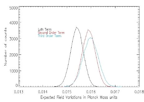
Figure 1: Distribution functions for the minimum excursion of the scalar field during inflation, $\Delta\phi_{h.c}$, for the three different slow roll expansions. Here, we have supposed a tensor-to-scalar ratio amplitude of the order of $\mu_{r}\sim 3\times 10^{-3}$ with $n_{s}=0.9680$, $\alpha_{s}=-0.0033$

Figure 2: Distribution functions for the variable $\Delta\phi_{h.c}$ for the three different slow roll expansions. In this case, we have supposed a detection of primordial GW of the order of $\mu_{r}\sim 5\times 10^{-3}$ with $n_{s}=0.9680$, $\alpha_{s}=-0.0033$

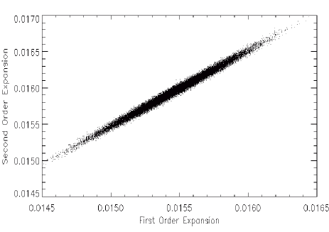
Figure 3: Dispersion plot for the ratio $\Delta\phi(\Pi_{1})/\Delta\phi(\Pi_{0})$ in the case of a detection of $r\sim 3\times 10^{-3}$ with $n_{s}=0.9680$, $\alpha_{s}=-0.0033$.

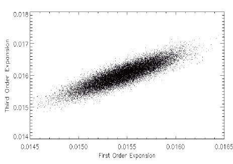
Figure 4: Dispersion plot for the ratio $\Delta\phi(\Pi_{2})/\Delta\phi(\Pi_{0})$ in the case of a detection of $r\sim 3\times 10^{-3}$ with $n_{s}=0.9680$, $\alpha_{s}=-0.0033$.

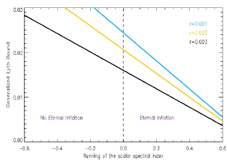
Figure 5: Third order Lyth Bound as a function of the running $\alpha_{s}$. In this case we consider $n_{s}\sim 0.9680$ with a threshold value $\alpha_{s}\sim-1.2842\times 10^{-5}$. Possible eternal inflation phases are associated with smaller variations of the field at horizon crossing of quantum fluctuations.

$\mu_{r}$	$\Delta\phi_{h.c}(\Pi_{0})$	$\Delta\phi_{h.c}(\Pi_{1})$	$\Delta\phi_{h.c}(\Pi_{2})$
$0.003$	$0.01545\pm 0.00026$	$0.01598\pm 0.00027$	$0.01605\pm 0.00028$
$0.004$	$0.01784\pm 0.00022$	$0.01846\pm 0.00024$	$0.01853\pm 0.00024$
$0.005$	$0.01995\pm 0.00019$	$0.02063\pm 0.00021$	$0.02072\pm 0.00022$

Table 1: Simulation results for the variation of the inflaton field at horizon crossing for the three different order of slow roll approximation. Here, the scalar spectral index and the relative running are fixed to $n_{s}=0.9650$ and $\alpha_{s}=-0.0025$, respectively. As one can see, the introduction of $n_{s}$ and $\alpha_{s}$ implies a larger excursion.

$\mu_{n_{s}}$	$\Delta\phi_{h.c}(\Pi_{1})$	$\Delta\phi_{h.c}(\Pi_{2})$
$0.9620$	$0.02069\pm 0.00021$	$0.02078\pm 0.00022$
$0.9650$	$0.02064\pm 0.00021$	$0.02071\pm 0.00022$
$0.9680$	$0.02058\pm 0.00021$	$0.02065\pm 0.00023$

Table 2: Simulation results for the variation of the inflaton field at horizon crossing for the second and third order of slow roll approximation. Here the tensor-to-scalar ratio is fixed to $r=0.005$ while the running is fixed to be $\alpha_{s}=-0.0025$. In this case, the variation of the field in which $n_{s}$ appears, become smaller as $n_{s}$ increases. This is due to the term $1-n_{s}$.

$\mu_{\alpha_{s}}$	$\Delta\phi_{h.c}(\Pi_{2})$
$-0.0005$	$0.02067\pm 0.00022$
$-0.0015$	$0.02069\pm 0.00022$
$-0.0025$	$0.02072\pm 0.00022$

Table 3: Simulation results for the variation of the inflaton field at horizon crossing for the three different values of the running $\alpha_{s}$. In this table we report the results for the higher order expression because is the only one in which $\alpha_{s}$ appears. The size of the variation is pushed toward smaller values (in modulus) for very low values of the running.

IV Theoretical implications and Conclusions

This analysis is performed using an extension of the standard Lyth formula for the variation of the field about the horizon crossing epoch of quantum modes. The computation of the expansion has been done likewise the local reconstruction of the effective inflationary potential around $\phi_{*}$ 36 . The first step is to introduce higher order terms in the slow roll picture and then, reword them in terms of the cosmological variables. In particular we derived a third order expansion for $\Delta\phi_{h.c}$. The Eq.(31) shows a linear dependence on $\alpha_{s}$ and it turns out to be decoupled by the other inflationary parameters. This is because there is not coupling between the third slow roll parameter, $\xi^{2}$, and the first two slow roll parameters [cfn. Eq.(21)]. It is straightforward to imagine that a hypothetical fourth order term will introduce a coupling between the running $\alpha_{s}$ and $r$ and $n_{s}$ and in addition it will introduce the higher order variables $d\alpha_{s}/d\ln k$. In this work, we performed Monte Carlo simulations assuming possible results of a single foreseen cosmological experiment. Morever, several new experiments have been proposed (see Sec. I for references). Therefore, we could combine the related results to get more accurate estimation on the main cosmological parameters ($r,n_{s},\alpha_{s}$), on some fundamental reheating variables (like the number of $e$-foldings during reheating stage $N_{reh}$ or the final reheating temperature, $T_{reh}$), and finally on $\Delta\phi_{h.c}$.
Mathematically, constraining the variation of the scalar field at horizon crossing is particularly important because provides a lower limit for the total excursion of the field. At the same time, we can observe the contribution of the observable quantities to $\Delta\phi$. Constraining little variations of $\Delta\phi_{h.c}$ in terms of $M_{p}$ (or $m_{p}$), does not imply a sub-Planckian total variation of field. This is because the last $e$-folds provides a large contribution on the total variation as reported in 3 . The size of the minimum variation of the scalar field can be related to a hypothetical eternal inflation. In the simplest scenario, following W.H.Kinney and K.Freese 35 , one can argue that a constant negative running $\alpha_{s}$ can prevent an eternal inflationary phase to occur. Since, at third order in the slow roll expansion, the variation of the field around the horizon crossing gets dependence in $\alpha_{s}$ we find that is possible to split $\Delta\phi_{H.c.}$ in two classes: one associated with the occurrence of the eternal inflation phase and one not. However, we should underline a couple of important questions about these results. First of all we do not have any guarantee that the function Eq.(35) is well described only by constant $\alpha_{s}$ (and $n_{s}$). In other words, we cannot be sure that a dramatic change (or not) of the order of magnitude about $P(s)$ is only related to the single running $\alpha_{s}$ parameter. In principle, the higher order terms may play an important role (see 35 ) and so we should generalize the procedure. On the other side, we cannot measure the running as well as any other cosmological variables outside our horizon, so it is also plausible that there is no observation can tell us if eternal inflation takes place or not. From this point of view, it is important to stress that a discussion about the relation between $\Delta\phi_{H.c.}$ and eternal inflation is still speculative. Surely, one can think that eternal inflation can be occur inside our horizon scale. In that case we should have observable consequences such as a natural and strong production of black holes. In our analysis we adopted a single field slow roll version of inflation as the paradigm of the early universe. This scenario could be confirmed and strengthened in the close future. Nevertheless there is still room (although little) for non-trivial signature of inflation. In this respect, the standard definition of Lyth Bound for the minimum variation of the scalar field is not more consistent as well as any kind of its slow roll generalizations. Then we need a new definition of $\Delta\phi$ during the horizon crossing of quantum fluctuations. This problem has been approached for example by Baumann and Green in 37 , in the context of general single field model ($P(X)$-model, 38 ) using the Goldstone picture of effective field theory of inflation (see 39 ).

- (1) A. H. Guth, “The Inflationary Universe: A Possible Solution to the Horizon and Flatness Problems,” Phys. Rev. D 23 (1981) 347; A. D. Linde, “A New Inflationary Universe Scenario: A Possible Solution of the Horizon, Flatness, Homogeneity, Isotropy and Primordial Monopole Problems,” Phys. Lett. 108B (1982) 389; A. Albrecht and P. J. Steinhardt, “Cosmology for Grand Unified Theories with Radiatively Induced Symmetry Breaking,” Phys. Rev. Lett. 48 (1982) 1220; S. W. Hawking and I. G. Moss, “Supercooled Phase Transitions in the Very Early Universe,” Phys. Lett. 110B (1982) 35; A. D. Linde, “Chaotic Inflation,” Phys. Lett. 129B (1983) 177.
- (2) D. H. Lyth, “What would we learn by detecting a gravitational wave signal in the cosmic microwave background anisotropy?,” Phys. Rev. Lett. 78 (1997) 1861 [hep-ph/9606387].
- (3) R. Easther, W. H. Kinney and B. A. Powell, “The Lyth bound and the end of inflation,” JCAP 0608 (2006) 004 [astro-ph/0601276].
- (4) D. H. Lyth and A. Riotto, “Particle physics models of inflation and the cosmological density perturbation,” Phys. Rept. 314 (1999) 1 [hep-ph/9807278]; G. Efstathiou and K. J. Mack, “The Lyth bound revisited,” JCAP 0505 (2005) 008 [astro-ph/0503360].
- (5) J. Garcia-Bellido, D. Roest, M. Scalisi and I. Zavala, “Can CMB data constrain the inflationary field range?,” JCAP 1409 (2014) 006 [arXiv:1405.7399 [hep-th]]; J. Garcia-Bellido, D. Roest, M. Scalisi and I. Zavala, “Lyth bound of inflation with a tilt,” Phys. Rev. D 90 (2014) no.12, 123539 [arXiv:1408.6839 [hep-th]].
- (6) Q. Gao, Y. Gong and T. Li, “Modified Lyth bound and implications of BICEP2 results,” Phys. Rev. D 91 (2015) 063509 [arXiv:1405.6451 [gr-qc]]; Q. G. Huang, “Lyth bound revisited,” Phys. Rev. D 91 (2015) no.12, 123532 [arXiv:1503.04513 [astro-ph.CO]].
- (7) A. Linde, “Gravitational waves and large field inflation,” JCAP 1702 (2017) no.02, 006 [arXiv:1612.00020 [astro-ph.CO]].
- (8) F. R. Bouchet et al. [COrE Collaboration], “COrE (Cosmic Origins Explorer) A White Paper,” arXiv:1102.2181 [astro-ph.CO]; F. Finelli et al. [CORE Collaboration], “Exploring Cosmic Origins with CORE: Inflation,” arXiv:1612.08270 [astro-ph.CO].
- (9) P. Andre et al. [PRISM Collaboration], “PRISM (Polarized Radiation Imaging and Spectroscopy Mission): A White Paper on the Ultimate Polarimetric Spectro-Imaging of the Microwave and Far-Infrared Sky,” arXiv:1306.2259 [astro-ph.CO].
- (10) J. Bock et al. [EPIC Collaboration], “Study of the Experimental Probe of Inflationary Cosmology (EPIC)-Intemediate Mission for NASA’s Einstein Inflation Probe,” arXiv:0906.1188 [astro-ph.CO].
- (11) A. Kogut et al., “The Primordial Inflation Explorer (PIXIE): A Nulling Polarimeter for Cosmic Microwave Background Observations,” JCAP 1107 (2011) 025 [arXiv:1105.2044 [astro-ph.CO]].
- (12) T. Matsumura et al., “Mission design of LiteBIRD,” J. Low. Temp. Phys. 176 (2014) 733 [arXiv:1311.2847 [astro-ph.IM]].
- (13) S. Phinney, et al., “The Big Bang Observer: Direct detection of gravitational waves from the birth of the universe to the present”, NASA mission concept study (2005); J. Crowder and N. J. Cornish, “Beyond LISA: Exploring future gravitational wave missions,” Phys. Rev. D 72 (2005) 083005 [gr-qc/0506015]; S. Chongchitnan and G. Efstathiou, “Prospects for direct detection of primordial gravitational waves,” Phys. Rev. D 73 (2006) 083511 [astro-ph/0602594]; H. Kudoh, A. Taruya, T. Hiramatsu and Y. Himemoto, “Detecting a gravitational-wave background with next-generation space interferometers,” Phys. Rev. D 73 (2006) 064006 [gr-qc/0511145].
- (14) P. A. R. Ade et al. [Planck Collaboration], “Planck 2015 results. XIII. Cosmological parameters,” Astron. Astrophys. 594 (2016) A13 [arXiv:1502.01589 [astro-ph.CO]].
- (15) P. A. R. Ade et al. [Planck Collaboration], “Planck 2015 results. XX. Constraints on inflation,” Astron. Astrophys. 594 (2016) A20 [arXiv:1502.02114 [astro-ph.CO]].
- (16) A. D. Linde, “Nonsingular Regenerating Inflationary Universe,” Print-82-0554 (CAMBRIDGE); P. J. Steinhardt “Natural Inflation” - 1983. in The Very Early Universe, G.W. Gibbons, S.W. Hawking, and S.T.C. Siklos (eds.) Cambridge University Press,, p. 251;
- (17) A. Vilenkin, “The Birth of Inflationary Universes,” Phys. Rev. D 27 (1983) 2848.
- (18) A. D. Linde, “Eternal Chaotic Inflation,” Mod. Phys. Lett. A 1 (1986) 81; A. D. Linde, “Eternally Existing Selfreproducing Chaotic Inflationary Universe,” Phys. Lett. B 175 (1986) 395; A. D. Linde, “Eternally Existing Selfreproducing Inflationary Universe,” Phys. Scripta T 15 (1987) 169.
- (19) A. S Goncharov, A. D. Linde, “Global structure of inflationary universe,” Zh. Eksp. Teor. Fiz. 92, 1137-1 150 (April 1987); A. S. Goncharov, A. D. Linde and V. F. Mukhanov, “The Global Structure of the Inflationary Universe,” Int. J. Mod. Phys. A 2 (1987) 561; A. D. Linde and A. Mezhlumian, “Stationary universe,” Phys. Lett. B 307 (1993) 25 [gr-qc/9304015]; A. D. Linde, D. A. Linde and A. Mezhlumian, “Nonperturbative amplifications of inhomogeneities in a selfreproducing universe,” Phys. Rev. D 54 (1996) 2504 [gr-qc/9601005]
- (20) F. L. Bezrukov and M. Shaposhnikov, “The Standard Model Higgs boson as the inflaton,” Phys. Lett. B 659 (2008) 703 [arXiv:0710.3755 [hep-th]].
- (21) A. A. Starobinsky, “A New Type of Isotropic Cosmological Models Without Singularity,” Phys. Lett. 91B (1980) 99.
- (22) L. A. Kofman, A. D. Linde and A. A. Starobinsky, “Inflationary Universe Generated by the Combined Action of a Scalar Field and Gravitational Vacuum Polarization,” Phys. Lett. 157B (1985) 361; M. B. Mijic, M. S. Morris and W. M. Suen, “The R**2 Cosmology: Inflation Without a Phase Transition,” Phys. Rev. D 34 (1986) 2934
- (23) D. Baumann, “Inflation,” arXiv:0907.5424 [hep-th].
- (24) E. Silverstein and A. Westphal, “Monodromy in the CMB: Gravity Waves and String Inflation,” Phys. Rev. D 78 (2008) 106003 [arXiv:0803.3085 [hep-th]].
- (25) L. McAllister, E. Silverstein and A. Westphal, “Gravity Waves and Linear Inflation from Axion Monodromy,” Phys. Rev. D 82 (2010) 046003 [arXiv:0808.0706 [hep-th]].
- (26) R. Kallosh, A. D. Linde, D. A. Linde and L. Susskind, “Gravity and global symmetries,” Phys. Rev. D 52 (1995) 912 [hep-th/9502069]; M. Kamionkowski and J. March-Russell, “Planck scale physics and the Peccei-Quinn mechanism,” Phys. Lett. B 282 (1992) 137 [hep-th/9202003].
- (27) R. Kallosh, A. D. Linde, D. A. Linde and L. Susskind, “Gravity and global symmetries,” Phys. Rev. D 52 (1995) 912 [hep-th/9502069].
- (28) A. D. Linde, “Prospects of inflation,” Phys. Scripta T 117 (2005) 40 [hep-th/0402051].
- (29) R. Kallosh and A. Linde, “Universality Class in Conformal Inflation,” JCAP 1307 (2013) 002 [arXiv:1306.5220 [hep-th]]; R. Kallosh and A. Linde, “Multi-field Conformal Cosmological Attractors,” JCAP 1312 (2013) 006 [arXiv:1309.2015 [hep-th]]; S. Ferrara, R. Kallosh, A. Linde and M. Porrati, “Minimal Supergravity Models of Inflation,” Phys. Rev. D 88 (2013) no.8, 085038 [arXiv:1307.7696 [hep-th]]; R. Kallosh and A. Linde, “Superconformal generalizations of the Starobinsky model,” JCAP 1306 (2013) 028 [arXiv:1306.3214 [hep-th]]; R. Kallosh, A. Linde and D. Roest, “Superconformal Inflationary -Attractors,” JHEP 1311 (2013) 198 [arXiv:1311.0472 [hep-th]]; M. Galante, R. Kallosh, A. Linde and D. Roest, “Unity of Cosmological Inflation Attractors,” Phys. Rev. Lett. 114 (2015) no.14, 141302 [arXiv:1412.3797 [hep-th]];
- (30) R. Kallosh and A. Linde, “Cosmological Attractors and Asymptotic Freedom of the Inflaton Field,” JCAP 1606 (2016) no.06, 047 [arXiv:1604.00444 [hep-th]];
- (31) A. R. Liddle, P. Parsons and J. D. Barrow, “Formalizing the slow roll approximation in inflation,” Phys. Rev. D 50 (1994) 7222 [astro-ph/9408015].
- (32) M. B. Hoffman and M. S. Turner, “Kinematic constraints to the key inflationary observables,” Phys. Rev. D 64 (2001) 023506 [astro-ph/0006321].
- (33) W. H. Kinney, “Inflation: Flow, fixed points and observables to arbitrary order in slow roll,” Phys. Rev. D 66 (2002) 083508 [astro-ph/0206032].
- (34) A. H. Guth, “Eternal inflation and its implications,” J. Phys. A 40 (2007) 6811 [hep-th/0702178 [HEP-TH]].
- (35) W. H. Kinney and K. Freese, “Negative running can prevent eternal inflation,” JCAP 1501 (2015) no.01, 040 [arXiv:1404.4614 [astro-ph.CO]].
- (36) J. E. Lidsey, A. R. Liddle, E. W. Kolb, E. J. Copeland, T. Barreiro and M. Abney, “Reconstructing the inflation potential : An overview,” Rev. Mod. Phys. 69 (1997) 373 [astro-ph/9508078].
- (37) D. Baumann and D. Green, “A Field Range Bound for General Single-Field Inflation,” JCAP 1205 (2012) 017 [arXiv:1111.3040 [hep-th]].
- (38) C. Armendariz-Picon, T. Damour and V. F. Mukhanov, “k - inflation,” Phys. Lett. B 458 (1999) 209 [hep-th/9904075]; X. Chen, M. x. Huang, S. Kachru and G. Shiu, “Observational signatures and non-Gaussianities of general single field inflation,” JCAP 0701 (2007) 002 [hep-th/0605045]; E. Silverstein and D. Tong, “Scalar speed limits and cosmology: Acceleration from D-cceleration,” Phys. Rev. D 70 (2004) 103505 [hep-th/0310221]; N. Arkani-Hamed, P. Creminelli, S. Mukohyama and M. Zaldarriaga, “Ghost inflation,” JCAP 0404 (2004) 001 [hep-th/0312100]; C. Burrage, C. de Rham, D. Seery and A. J. Tolley, “Galileon inflation,” JCAP 1101 (2011) 014 [arXiv:1009.2497 [hep-th]]
- (39) C. Cheung, P. Creminelli, A. L. Fitzpatrick, J. Kaplan and L. Senatore, “The Effective Field Theory of Inflation,” JHEP 0803 (2008) 014 [arXiv:0709.0293 [hep-th]]; L. Senatore and M. Zaldarriaga, “The Effective Field Theory of Multifield Inflation,” JHEP 1204 (2012) 024 [arXiv:1009.2093 [hep-th]]; P. Creminelli, M. A. Luty, A. Nicolis and L. Senatore, “Starting the Universe: Stable Violation of the Null Energy Condition and Non-standard Cosmologies,” JHEP 0612 (2006) 080 [hep-th/0606090]; N. Bartolo, M. Fasiello, S. Matarrese and A. Riotto, “Large non-Gaussianities in the Effective Field Theory Approach to Single-Field Inflation: the Bispectrum,” JCAP 1008 (2010) 008 [arXiv:1004.0893 [astro-ph.CO]]. N. Bartolo, M. Fasiello, S. Matarrese and A. Riotto, “Large non-Gaussianities in the Effective Field Theory Approach to Single-Field Inflation: the Trispectrum,” JCAP 1009 (2010) 035 [arXiv:1006.5411 [astro-ph.CO]].